Space-Time Decomposition of Kalman Filter

Abstract

We present an innovative interpretation of Kalman Filter (KF, for short) combining the ideas of Schwarz Domain Decomposition (DD) and Parallel in Time (PinT) approaches. Thereafter we call it DD-KF. In contrast to standard DD approaches which are already incorporated in KF and other state estimation models, implementing a straightforward data parallelism inside the loop over time, DD-KF ab-initio partitions the whole model, including filter equations and dynamic model along both space and time directions/steps. As a consequence, we get local KFs reproducing the original filter at smaller dimensions on local domains. Also, sub problems could be solved in parallel. In order to enforce the matching of local solutions on overlapping regions, and then to achieve the same global solution of KF, local KFs are slightly modified by adding a correction term keeping track of contributions of adjacent subdomains to overlapping regions. Such a correction term balances localization errors along overlapping regions, acting as a regularization constraint on local solutions. Furthermore, such a localization excludes remote observations from each analyzed location improving the conditioning of the error covariance matrices. As dynamic model we consider Shallow Water equations which can be regarded a consistent tool to get a proof of concept of the reliability assessment of DD-KF in monitoring and forecasting of weather systems and ocean currents.

Keywords: Data Assimilation, Kalman Filter, Domain Decomposition, Filter Localization, Model Reduction, Numerical Algorithm.
AMS:35Q93,49M27, 49M41, 65K15, 65M32

1 Introduction

In the present paper we focus on Kalman Filter (KF) which is one of the most important and common state estimation algorithms solving Data Assimilation (DA) problems Kalman; Kalnay. Besides its employment in validation of mathematical models used in meteorology, climatology, geophysics, geology and hydrology Wu, it has become a main component in visual tracking of moving object in image processing or autonomous vehicles tracking with GPS in satellite navigation systems, or even in applications of non physical systems such as financial markets Karavasilis; Benhamou; Heidari; Wu. Its main strength is the simple derivation of the algorithm using the filter recursive property: measurements/observations are processed step by step as they arrive allowing to correct the given data. A recent review of KF and its applications is given in Kim.
KF time complexity requires very large computational burden in concrete scenarios Lyster; Tang; Tossavainen. Hence, several variants/approximation have been proposed to reduce the computational complexity and to allow KF deployment in real time. These are designed on the basis of a reduction in the order of the model Hahnel; Hannachi; Rozier; Wikle, or they are based on Ensemble Kalman Filter (EnKF) which approximates KF by representing the distribution of the state with an ensemble of draws from that distribution. A prediction of the error at a future time is computed by integrating each ensemble state independently by the model Evensen. EnKF can be used for nonlinear dynamics settings and they are more suited to large scale real world problems than the KF, so it is more viable for use within operational DA Sandu. Nevertheless, EnKF methods are hindered by a reduction in the size of the ensemble due to the computational requirements of maintaining a large ensemble Anderson; Hamill. In applications, most efforts to deal with the related problems of computational effort and sampling error in ensemble estimation have focused on using variations on the concept of localization Zhou.
A typical approach for solving computationally intensive problems - which is oriented to exploit parallel computing - is based on Schwarz Domain Decomposition (DD) techniques. DD methods are well-established strategies that has been used with great success for a wide variety of problems. Review papers, both for mathematical and computational analysis are for instance Meurant; Quarteroni; Saad; Schwarz. Concerning DA problems, DD is usually performed by discretizing the objective function and the model to build a discrete Lagrangian DD-DA. At the heart of these so called all-at-once approaches, lies solution of a very large linear system (the Karush-Kuhn-Tucker (KKT) system) which is decomposed according to the discretization grid. A common drawback of such parallel algorithms is their limited scalability, due to the fact that parallelism is achieved adapting the most computationally demanding tasks for parallel execution. Concerning KF this approach leads to the straightforward data parallelism inside the loop over time-steps. Amdhal’s Law clearly applied in these situations because the computational cost of the components that are not parallelized - or in case of KF a data synchronization at each step - provides a lower bound on the execution time of the parallel algorithm. More generally if a fraction $r$ of our serial program remains unparallelized, then Amdahl’s Law says we can’t get a speedup better than $1/r$. Thus even if r is quite small, say 1/100, and we have a system with thousands of cores, we can’t get a speedup better than 100.

Here we present the mathematical framework of an innovative approach which turns to be appropriate for using state estimation problems described by KF and governed by a dynamic model such as Partial Differential Equations (PDEs). This approach relies on the ideas of Schwarz DD Schwarz and Parallel in Time (PinT) approaches Lions fully revised in a linear algebra setting. Schwarz methods use as boundary conditions of the local PDE-model the approximation of the numerical solution computed on the interfaces between adjacent spatial subdomains. In order to introduce a consistent DD along the time direction, PinT methods use a coarse/global/predictor propagator to obtain approximate initial values of local models on the coarse time-grid; a fine/local/corrector solver to obtain the solution of local models starting from the approximate initial values; an iterative procedure to smooth out the discontinuities of the global model on the overlapping domains. Nevertheless, one of the key limitation of any PinT-based methods is data dependencies of the local solvers from the coarse solver: the coarse solver must always be executed serially for the full duration of the simulation and local solver have to wait for the approximate initial values provided by the coarse solver. We use the KF solution as coarse predictor for the local PDE-based model, providing the approximations needed for locally solving the initial value problems on each time subinterval, whereas the PDE model serves as a fine description which locally improves the coarse one, on each time interval in order to iteratively improve the first prediction.
We underline that the idea of partitioning the spacial domain into sub-domains and use KF on these subdomains for a fixed time is quite old, as it goes back to Lorenc in 1981 Lorenc1981. This is essentially the idea underlying domain localization which has been deeply investigated in applications (see for instance Brankart; Brusdal; Haugen; Nerger2006; Ott). Because the assimilations are performed independently in each local region, two neighboring subdomains might produce strongly different analysis estimates when the assimilated observations have gaps. Our approach instead resolves both the inherent bottleneck of time–marching solvers and the smoothness problem of the analysis fields.

We emphasize that there is a quite different rationale behind such DD framework and the so called Model Order Reduction (MOR) methods, even though they are closely related each other. The primary motivation of DD methods based on Additive Schwarz Method (ASM) was the inherent parallelism arising from a flexible, adaptive and independent decomposition of the given problem into several sub problems, though they can also reduce the complexity of sequential solvers. ASM algorithms and theoretical frameworks are, to date, the most mature for this class of problems. MOR techniques are based on projection of the full order model onto a lower dimensional space spanned by a reduced order basis. These methods has been used extensively in a variety of fields for efficient simulations of highly intensive computational problems. But all numerical issues concerning the quality of approximation still are of paramount importance Petzold. As previously mentioned, DD-KF framework makes it natural to switch from a full scale solver to a model order reduction solver for solution of subproblems for which no relevant low-dimensional reduced space should be constructed. In the same way, DD-KF framework leads to the model decomposition in space and time which is coherent with the filter localization. In conclusion, main advantage of the DD-KF is to combine in one theoretical framework, model decomposition, along the space dimension and time steps, and filter itself, while providing a flexible, adaptive, reliable and robust decomposition.

Summarizing, we partition initial domain along space dimension and time steps, then we extend each subdomain to overlap its neighbors by an amount; partitioning can be adapted according to the availability of measurements and data DyDD. Accordingly, we decompose forecasting model both in space and time. In particular, it means that as initial and boundary values of local forecasting models, according to Parallel in Time and Schwarz domain decomposition idea, we use estimates provided by KF itself at previous step in the adjacent space-time interval, as soon as these are computed. On each subdomain we formulate a local KF problem analogous to the original one, defined on local models. In order to enforce the matching of local solutions on overlapping regions, local KF problems are slightly modified by adding a correction term, acting as a smoothness-regularization constraint on local solutions, which keeps track of contributions of adjacent domains to overlapping regions; the same correction is applied to covariance matrices, thereby improving the conditioning of the error covariance matrices.
To the best of our knowledge, such an ab-initio decomposition of KF along space and time steps has never been investigated before. A spatially distributed KF into sensor based reduced-order models, implemented on a sensor networks where multiple sensors are mounted on a robot platform for target tracking, is presented in Battistelli; Khan. A new algorithm only using domain localization in Extended Kalman Filter is proposed in Janic.

We would like to mention that in the present work we derive and discuss main features of DD-KF framework using the Shallow Water Equations (SWEs) which are commonly used for monitoring and forecasting the water flow in rivers and open channels (see for instance Rafiee; Tirupachi). Nevertheless, as we follow the first discretize then optimize approach, Schwarz and PinT methods are completely revisited in the linear algebra setting of this framework, allowing its application in the plentiful literature of state estimation real-world problems. We observe that the same authors have presented a simplified version of DD-KF in PPAM2019, where KF was used for solving CLS (Constrained Least Square) models, seen as prototype model of Data Assimilation problems. CLS is obtained combining two overdetermined linear systems, representing the state and the observation mapping.
The rest of the article is organized as follows. In section §2, we review preliminaries on KF then in section §3 we describe DD-KF framework and its related algorithm. In section 4, we define the mathematical framework underlying DD-KF. In section §5, we theoretically prove its reliability while validation on the Shallow Water Equations are given in section §6. Conclusions and possible extensions are provided in section §7. Finally, with the aim of allowing replicability of experimental results section §8 contains the whole detailed derivation of DD-KF method on SWEs and performance analysis of DD-KF w.r.t. KF.

2 Preliminaries on Kalman Filter

Given $x_{0}\in\mathbb{R}^{N}$, let $x(t)\in\Omega\subset\mathbb{R}^{N}$, where $\forall t\in\Delta$, denote the state of a dynamic system governed by the mathematical model $\mathcal{M}_{t,t+\Delta t}(x(t))$, such that:

$$\left\{\begin{array}[]{ll}x(t+\Delta t)&=\mathcal{M}_{t,t+\Delta t}(x(t)),\\ x(0)&=x_{0}\end{array},\right.$$ (1)

and let:

$$y(t+\Delta t)=\mathcal{H}_{t+\Delta t}[x(t+\Delta t)],$$ (2)

denote the so called observations, where

$$\mathcal{H}_{t+\Delta t}:\ x(t+\Delta t)\in\mathbb{R}^{n}\mapsto y(t+\Delta t)\in\mathbb{R}^{d}\,,\quad d\in\mathbb{N}\quad d<<N\,,$$ (3)

denotes the observations mapping including transformations and grid interpolations. Here we may assume that both $\mathcal{M}$ and $\mathcal{H}$ are non linear.
In the context of DA methods, KF aims to bring the state $H(x(t))$ as close as possible to the measurements/observations $y(t)$. One can do this by discretizing then optimize or first optimize and then discretize. Here, with the aim of making the best use of Schwarz and PinT methods in a linear algebra settings, we first discretize then optimize.
Let $r\in\mathbb{N}$ be given. We consider $r+2$ points in $\Delta$, let us say $\{t_{k}\}_{k=0,1,\ldots,r+1}$, where $t_{k}=k\Delta t$ and $\Delta t=\frac{T}{r+1}$ (more in general, the mesh $t_{k}$ need not be uniform).
We use the following setup of KF: $x_{k}\equiv x(t_{k})$, state at $t_{k}$; $x_{0}$: state at $t_{0}\equiv 0$ (or the vector of initial conditions); $M_{k,k+1}\in\mathbb{R}^{N\times N}$: discretization of the tangent linear operator (Jacobian) of $\mathcal{M}_{t,t+\Delta t}(x(t))$; $m\in\mathbb{N}$: number of observations; $y_{k}\equiv y(t_{k})\in\mathbb{R}^{m\cdot d}$: observations vector; $b_{k}\in\mathbb{R}^{N}$: input control vector; $H_{k+1}\in\mathbb{R}^{m\cdot d\times N}$: discretization of tangent linear approximation of $\mathcal{H}_{t_{k+1}}$ (also called observations operator) with $N>m$, for $k=0,1,\ldots,r$; $w_{k}\in\mathbb{R}^{n}$ and $v_{k}\in\mathbb{R}^{m\cdot d}$: model and observation additive errors with normal distribution and zero mean; $Q_{k}\in\mathbb{R}^{N\times N}$ and $R_{k}\in\mathbb{R}^{m\cdot d\times m\cdot d}$: covariance matrices of the errors on the model and on the observations, such that

$$Q_{k}:=E[w_{k}w_{k}^{T}]\quad R_{k}:=E[v_{k}v_{k}^{T}]\quad\textit{$\forall$ $k=0,1,\ldots,r+1$}.$$ (4)

where $E[\cdot]$ denotes the expected value, $\forall k=0,1,\ldots,r$. These matrices are symmetric and positive definite.

KF consists in the iterative estimate of $x_{k+1}\in\mathbb{R}^{n}$:

$$x_{k+1}=M_{k,k+1}x_{k}+b_{k}+w_{k},\quad$$ (5)

such that

$$y_{k+1}=H_{k+1}{x}_{k+1}+v_{k+1}\quad.$$ (6)

An example of the vector $b_{k}$ is given for the Shallow Water Equations described in the Appendix (see (92)).

If $P_{0}\in\mathbb{R}^{n\times n}$ and $\widehat{x}_{0}:=x_{0}$, each step of KF is composed by two main operations sorenson.

• Predictor phase, involving computation of state estimate:

  $$x_{k+1}=M_{k,k+1}\widehat{x}_{k}+b_{k};$$ (7)

  computation of covariance matrices:

  $$P_{k+1}= M_{k,k+1}P_{k}M_{k,k+1}^{T}+Q_{k}$$ (8)

  $$S_{k+1}= H_{k+1}P_{k+1}H_{k+1}^{T}+R_{k+1}$$

  and computation of KF gain:

  $$K_{k+1}=P_{k+1}H_{k+1}^{T}S_{k+1}^{-1}.$$ (9)

• Corrector phase, involving the update of covariance matrix:

  $$P_{k+1}=(I-K_{k+1}H_{k+1})P_{k+1},$$ (10)

  and the update of state estimate:

  $$\widehat{x}_{k+1}=x_{k+1}+K_{k+1}(y_{k+1}-H_{k+1}x_{k+1}).$$ (11)

3 DD-KF

Let $D_{n}(\Omega)=\{{x}_{j}\}_{j=1,\ldots,n}$, be the mesh partitioning of $\Omega$ and $b_{c}\in\mathbb{N}$ such that $D_{b_{c}}(\partial\Omega)=\{{z}_{p}\}_{p=1,\ldots,b_{c}}$ be the discretization of $\partial\Omega$. If we let $x_{k+1}^{\partial\Omega}\in\mathbb{R}^{b_{c}}$ to be the state at $t_{k+1}$ on $\partial\Omega$, it is

$$x_{k+1}^{\partial\Omega}\equiv x^{\partial\Omega}(t_{k+1})\in\mathbb{R}^{b_{c}}.$$ (12)

DD-KK consists of two main steps, namely domain decomposition and model decomposition. In the following, for simplicity of notation, and without loss of generality we consider two spatial subdomains, while the general case involving more than two subdomains will be briefly described in section 3.1.1.

DD in space. Let $\Omega_{1}$, $\Omega_{2}\subset\Omega$ such that

$$\Omega=\Omega_{1}\cup\Omega_{2}$$ (13)

with $D_{n_{1}}(\Omega_{1}),D_{n_{2}}(\Omega_{2})\subset D_{n}(\Omega)$, where $n_{i}<n$ are such that

$$D_{n_{1}}(\Omega_{1})=\{x_{i}\}_{i\in I_{1}}\quad,\quad D_{n_{2}}(\Omega_{2})=\{x_{i}\}_{i\in I_{2}}$$ (14)

and $n_{1}=|D_{n_{1}}(\Omega_{1})|$, $n_{2}=|D_{n_{2}}(\Omega_{2})|$; let

$$\Omega_{1,2}:=\Omega_{1}\cap\Omega_{2},$$ (15)

be the overlap region where we introduce

$$D_{s}(\Omega_{1,2}):=D_{n_{1}}(\Omega_{1})\cap D_{n_{2}}(\Omega_{2})=\{x_{i}\}_{i\in I_{1,2}}$$ (16)

denoting the discretization of $\Omega_{1,2}$ and

$$I_{1}=\{1,\ldots,n_{1}\},\quad I_{2}=\{n_{1}-s+1,\ldots,n\},\quad I_{1,2}=\{n_{1}-s+1,\ldots,n_{1}\}$$ (17)

are the corresponding index sets, with $s\in\mathbb{N}_{0}$.

DD in time. Let $\Delta_{j}\subset\Delta$ such that

$$\Delta=\cup_{j=1}^{L}\Delta_{j}\,.$$ (18)

Let $D_{s_{j}}(\Delta_{j})\subset D_{r+2}(\Delta)$ be such that

$$D_{s_{j}}(\Delta_{j})=\{t_{k}\}_{k=\bar{s}_{j-1},\ldots,\bar{s}_{j-1}+s_{j}}$$ (19)

denoting the discretization of $\Delta_{j}$, where in (19) the quantity

$$\bar{s}_{j-1}:=\sum_{l=1}^{j-1}(s_{l}-s_{l-1,l}),\quad s_{j-1,j}\in\mathbb{N}_{0}$$ (20)

is the number of elements in common between subsets $\Delta_{j-1}$ and $\Delta_{j}$, and it is such that $s_{0}:=0$, $s_{0,1}:=0$ and $\bar{s}_{L-1}+s_{L}:=r+1$, then

$$\Delta_{j-1,j}:=\Delta_{j-1}\cap\Delta_{j},$$ (21)

with

$$D_{s_{j-1,j}}(\Delta_{j-1,j}):=D_{s_{j-1}}(\Delta_{j-1})\cap D_{s_{j}}(\Delta_{j})$$

denoting the discretization of the overlapping time interval.

The innovative idea is to split the outer loop of KF (let us say, the time - step loop along $k=1,\ldots,r$) in $L$ parts each one running in $\Delta_{j}$ (where $j=1,\ldots,L$) as described below.

For $j=1,\ldots,L$, let us indicate by $\widehat{x}_{k+1}^{\Delta_{j}}$, the KF solution such that:

$$\widehat{x}_{k+1}^{\Delta_{j}}=M_{k,k+1}\widehat{x}_{k}^{\Delta_{j}}+b_{k}+w_{k},\quad\forall k=\bar{s}_{j-1},\ldots,\bar{s}_{j-1}+s_{j}-1$$ (22)

where

$$\widehat{x}_{\bar{s}_{j-1}}^{\Delta_{j}}=\widehat{x}_{\bar{s}_{j-1}}^{\Delta_{j-1}}$$ (23)

is the initial value such that (according to DA condition):

$$y_{k+1}=H_{k+1}\widehat{x}_{k+1}^{\Delta_{j}}+v_{k+1},$$ (24)

in particular it is $\widehat{x}_{0}^{\Delta_{0}}:=x_{0}$. We note in (23) that according to PinT compatibility conditions initial value at $\Delta_{j}$ is the estimate computed at previous step in $\Delta_{j-1}$.

We now consider the following block partitioning of $M:=M_{k,k+1}\in\mathbb{R}^{n\times n}$ and $H_{k+1}\in\mathbb{R}^{m\cdot d\times n}$:

$$M=\left[\begin{array}[]{c|c}M_{1}&M_{1,2}\\ \hline\cr M_{2,1}&M_{2}\end{array}\right],$$ (25)

and

$$H_{k+1}=\left[H_{k+1}^{1}\ H_{k+1}^{2}\right].$$ (26)

In particular,

• if $s=0$ (no overlap), for $i,j=1,2$:

  $$M_{i}:=M|_{I_{i}\times I_{i}}\in\mathbb{R}^{n_{i}\times n_{i}}\quad M_{i,j}:=M|_{I_{i}\times I_{j}}\in\mathbb{R}^{n_{i}\times n_{j}},$$ (27)

  and

  $$H_{k+1}^{1}:=H_{k+1}|_{I_{1}}\in\mathbb{R}^{m\cdot d\times n_{1}},\quad H_{k+1}^{2}:=H_{k+1}|_{I_{2}}\in\mathbb{R}^{m\cdot d\times n_{2}},$$ (28)

• while if $s\neq 0$ (in presence of overlapping region), we have:

  $$\begin{array}[]{lllllll}\mathbb{M}_{1,1}&:=M|_{\tilde{I}_{1}\times\tilde{I}_{1}}\in\mathbb{R}^{(n_{1}-s)\times(n_{1}-s)},\quad\mathbb{M}_{1,2}&:=M|_{\tilde{I}_{1}\times{I}_{1,2}}\in\mathbb{R}^{(n_{1}-s)\times s},\\ \mathbb{M}_{1,3}&:=M|_{\tilde{I}_{1}\times\tilde{I}_{2}}\in\mathbb{R}^{(n_{1}-s)\times(n_{2}-s)},\quad\par\mathbb{M}_{2,1}&:=M|_{{I}_{1,2}\times\tilde{I}_{1}}\in\mathbb{R}^{s\times(n_{1}-s)},\\ \mathbb{M}_{2,2}&:=M|_{{I}_{1,2}\times{I}_{1,2}}\in\mathbb{R}^{s\times s},\quad\ \ \ \ \ \ \ \ \ \ \ \mathbb{M}_{2,3}&:=M|_{{I}_{1,2}\times\tilde{I}_{2}}\in\mathbb{R}^{s\times(n_{2}-s)},\\ \mathbb{M}_{3,1}&:=M|_{\tilde{I}_{2}\times\tilde{I}_{1}}\in\mathbb{R}^{(n_{2}-s)\times(n_{1}-s)},\quad\mathbb{M}_{3,2}&:=M|_{\tilde{I}_{2}\times{I}_{1,2}}\in\mathbb{R}^{(n_{2}-s)\times s},\\ \mathbb{M}_{3,3}&:=M|_{\tilde{I}_{2}\times\tilde{I}_{2}}\in\mathbb{R}^{(n_{2}-s)\times(n_{2}-s)}.\end{array}$$

  Then in (25) we have:

  $$\begin{array}[]{lllllllllll}M_{1}:=\left[\begin{array}[]{cc}\mathbb{M}_{1,1}&\mathbb{M}_{1,2}\\ \mathbb{M}_{2,1}&\mathbb{M}_{2,2}\end{array}\right],\quad{M}_{1,2}:=\left[\begin{array}[]{cc}0&\mathbb{M}_{1,3}\\ 0&\mathbb{M}_{2,3}\end{array}\right],\\ {M}_{2,1}:=\left[\begin{array}[]{cc}\mathbb{M}_{2,1}&0\\ \mathbb{M}_{3,1}&0\end{array}\right],\quad M_{2}:=\left[\begin{array}[]{cc}\mathbb{M}_{2,2}&\mathbb{M}_{2,3}\\ \mathbb{M}_{3,2}&\mathbb{M}_{3,3}\end{array}\right],\end{array}$$ (29)

  and

  $$H_{k+1}^{1}:=\left[H_{k+1}^{1,1}\ \ \alpha H_{k+1}^{1,2}\right],\quad H_{k+1}^{2}:=\left[\beta H_{k+1}^{1,2}\ \ H_{k+1}^{2,2}\right],$$ (30)

  with:

  $$H_{k+1}^{1,1}:=H_{k+1}|_{\tilde{I}_{1}},\quad H_{k+1}^{2,2}:=H_{k+1}|_{\tilde{I}_{2}},\quad H_{k+1}^{1,2}:=H_{k+1}|_{{I}_{1,2}},$$ (31)

  where

  $$\tilde{I}_{1}:=I_{1}\setminus{I}_{1,2},\quad\tilde{I}_{2}:=I_{2}\setminus{I}_{1,2},$$ (32)

  and $n_{1}-s=|\tilde{I}_{1}|$, $n_{2}-s=|\tilde{I}_{2}|$. We note that in (30), in presence of overlapping region, it should be $\alpha H_{k+1}^{1,2}+\beta H_{k+1}^{1,2}=H_{k+1}|_{{I}_{1,2}}$, so we require that $\alpha+\beta=1$.

We highlight that DD-KF employs a block partitioning of $M$ as in the Additive Schwarz DD, while as in the PinT approach, initial value of restricted models are the KF estimates computed at previous step. In particular, at $t_{0}\equiv 0$, DD-KF in $\Delta_{1}$ employs as initial value $x_{0}\equiv\widehat{x}_{0}$ which is the initial condition of the dynamic model appropriately restricted to $\Omega_{1}$ or $\Omega_{2}$.

In Fig. 1 we report a schematic description of how DD-KF trajectory is decomposed in two spatial subdomains and six time subdomains.

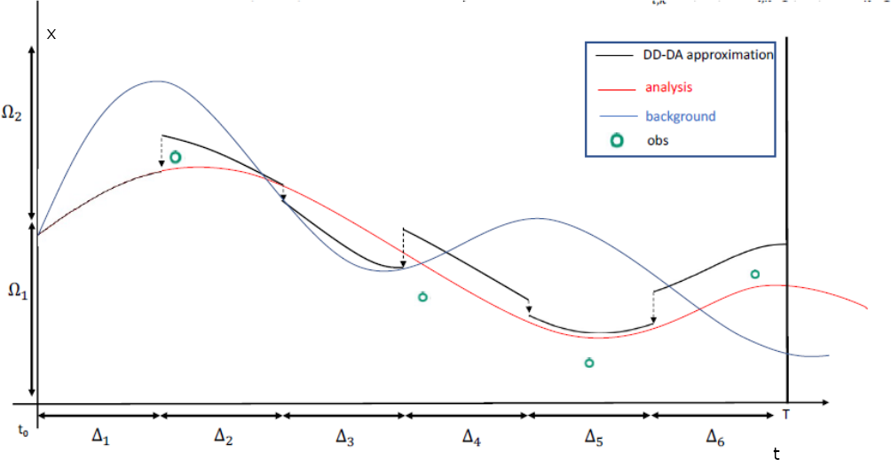
Figure 1: Schematic description of DD-KF solution trajectory for $N=1$, that is $\Omega$ is a subset of $\Re$ and is splitted in two sub domains (represented along the x-axis), while the time interval is splitted in six sub intervals (represented along the t-axis).

That said, we now consider local KF problems in $\Delta_{j}\subset\Delta$.

Definition 1

(Local KF problems) KF problems in $\Delta_{j}\times\Omega_{1}$ and $\Delta_{j}\times\Omega_{2}$ are, $\forall\,k=\bar{s}_{j-1},\ldots,\bar{s}_{j-1}+s_{j}-1$, the following:

$$P_{\Omega_{1}}^{\Delta_{j}}:\ \ \left\{\begin{array}[]{ll}x_{1,k+1}^{\Delta_{j}}=M_{1}x_{1,k}^{\Delta_{j}}+b_{k}|_{I_{1}}+b_{1,k}+w_{k}|_{I_{1}}\\ y_{k+1}=H_{k+1}^{1}{x}_{1,k+1}^{\Delta_{j}}+H_{k+1}^{2}{x}_{2,k+1}^{\Delta_{j}}+v_{k+1}\end{array}\right.$$ (33)

and

$$P_{\Omega_{2}}^{\Delta_{j}}:\ \ \left\{\begin{array}[]{ll}x_{2,k+1}^{\Delta_{j}}=M_{2,1}x_{1,k}^{\Delta_{j}}+b_{k}|_{I_{2}}+b_{2,k}+w_{k}|_{I_{2}}\\ y_{k+1}=H_{k+1}^{1}{x}_{1,k+1}^{\Delta_{j}}+H_{k+1}^{2}{x}_{2,k+1}^{\Delta_{j}}+v_{k+1}\end{array},\right.$$ (34)

with initial states

$$x_{1,\bar{s}_{j-1}}^{\Delta_{j}}=x_{1,\bar{s}_{j-1}}^{\Delta_{j-1}}\quad x_{2,\bar{s}_{j-1}}^{\Delta_{j}}=x_{2,\bar{s}_{j-1}}^{\Delta_{j-1}}.$$ (35)

In particular it is $x_{1,\bar{s}_{0}}^{\Delta_{0}}:=x_{0}|_{I_{1}}$, $x_{2,\bar{s}_{0}}^{\Delta_{0}}:=x_{0}|_{I_{2}}$ and

$$\begin{array}[]{ll}x_{1,k}^{\Delta_{j}}|_{\partial\Omega_{1}\setminus\Omega_{2}}={x}_{k}^{\partial\Omega_{1}\setminus\Omega_{2}}\\ x_{1,k}^{\Delta_{j}}|_{\Gamma_{1}}=x_{2,k}|_{\Gamma_{1}}\end{array}\quad\begin{array}[]{ll}x_{2,k}^{\Delta_{j}}|_{\partial\Omega_{2}\setminus\Omega_{1}}={x}_{k}^{\partial\Omega_{2}\setminus\Omega_{1}}\\ x_{2,k}^{\Delta_{j}}|_{\Gamma_{2}}=x_{1,k}|_{\Gamma_{2}}\end{array}$$ (36)

where

$$\Gamma_{1}:=\partial\Omega_{1}\cap\Omega_{2}\quad,\quad\Gamma_{2}:=\partial\Omega_{2}\cap\Omega_{1}\\$$ (37)

and

$$b_{1,k}:=\left[\begin{array}[]{ll}\mathbb{M}_{1,3}\\ \mathbb{M}_{2,3}\end{array}\right]x_{2,k}^{\Delta_{j}}|_{\Gamma_{1}}\quad b_{2,k}:=\left[\begin{array}[]{ll}\mathbb{M}_{2,1}\\ \mathbb{M}_{3,1}\end{array}\right]x_{1,k}^{\Delta_{j}}|_{\Gamma_{2}}.$$ (38)

$H_{k}^{1}\in\mathbb{R}^{m\cdot d\times n_{1}}$ and $H_{k}^{2}\in\mathbb{R}^{m\cdot d\times n_{2}}$ are defined in (30) and, for $i=1,2$, $x_{\bar{s}_{j-1}}^{\Delta_{j-1}}|_{I_{i}}$ and $w|_{I_{i}}$ are reductions to $I_{i}$ of $\widehat{x}_{0}\in\mathbb{R}^{n}$ and $w\in\mathbb{R}^{n}$. As a consequence, the errors

$$e_{1,k+1}:=(x_{1,k+1}-x_{1,k})\in\mathbb{R}^{n_{1}},\quad e_{2,k+1}:=(x_{2,k+1}-x_{1,k})\in\mathbb{R}^{n_{2}}$$

defined in $\Omega_{1}$ and $\Omega_{2}$, give the local estimate of

$$P_{i,j}:=Cov(e_{i,k+1},e_{j,k+1})$$

with $i\neq j$. Similarly,

$$\begin{array}[]{ll}Q_{k}&=diag(Q_{1,k},Q_{2,k})\in\mathbb{R}^{n\times n}\\ \end{array}$$ (39)

and $D_{k}\in\mathbb{R}^{m\cdot d\times m\cdot d}$ are local covariance matrices of errors on model and on observations where, $Q_{1,k}\in\mathbb{R}^{n_{1}\times n_{1}}$ and $Q_{2,k}\in\mathbb{R}^{n_{2}\times n_{2}}$, while $D_{k}$ is a diagonal matrix.

We note that the local aspect of the KF problem given in Definition 2 comes out from both the local contribution of the model and from the filter localization.

3.1 Local problems

In the following we let $\Delta_{j}$ be fixed, then for simplicity of notation, we refer to $\widehat{x}_{i,k}^{\Delta_{j}}$ omitting superscript $\Delta_{j}$. $\forall k=\bar{s}_{j-1},\ldots,\bar{s}_{j-1}+s_{j}-1$ local problems are made of:

• Predictor phase. Computation of state estimates:

  $$\begin{array}[]{ll}x_{1,k+1}=M_{1}\widehat{x}_{1,k}+b_{k}|_{I_{1}}+b_{1,k}+w_{k}|_{I_{1}}\\ x_{2,k+1}=M_{2}\widehat{x}_{2,k}+b_{k}|_{I_{2}}+b_{2,k}+w_{k}|_{I_{2}}\end{array};$$ (40)

  where

  $$b_{1,k}:=\left[\begin{array}[]{ll}\mathbb{M}_{1,3}\\ \mathbb{M}_{2,3}\end{array}\right]\widehat{x}_{2,k}|_{\Gamma_{1}}\quad b_{2,k}:=\left[\begin{array}[]{ll}\mathbb{M}_{2,1}\\ \mathbb{M}_{3,1}\end{array}\right]\widehat{x}_{1,k}|_{\Gamma_{2}};$$ (41)

  computation of the local estimate of

  $$\begin{array}[]{ll}P_{1}=M_{1}P_{1}M_{1}^{T}+P_{\Omega_{1}\leftrightarrow\Omega_{2}}+Q_{1,k}\\ P_{2}=M_{2}P_{2}M_{2}^{T}+P_{\Omega_{2}\leftrightarrow\Omega_{1}}+Q_{2,k}\end{array},$$ (42)

  where

  $$\begin{array}[]{ll}P_{\Omega_{1}\leftrightarrow\Omega_{2}}=M_{1,2}P_{2,1}M_{1}^{T}+M_{1}P_{1,2}M_{1,2}^{T}+M_{1,2}P_{2}M_{1,2}^{T}\\ P_{\Omega_{2}\leftrightarrow\Omega_{1}}=M_{2,1}P_{1,2}M_{2}^{T}+M_{2}P_{2,1}M_{2,1}^{T}+M_{2,1}P_{1}M_{2,1}^{T}\end{array},$$ (43)

  with

  $$\begin{array}[]{ll}P_{1,2}=M_{1}P_{1,2}M_{2}^{T}+C_{\Omega_{1}\leftrightarrow\Omega_{2}}\\ P_{2,1}=M_{2}P_{2,1}M_{1}^{T}+C_{\Omega_{1}\leftrightarrow\Omega_{2}}^{T}\end{array},$$ (44)

  and

  $$\begin{array}[]{ll}C_{\Omega_{1}\leftrightarrow\Omega_{2}}=M_{1}P_{1}M_{2,1}^{T}+M_{1,2}P_{2,1}M_{2,1}^{T}+M_{1,2}P_{2}M_{2}^{T}\end{array}$$ (45)

  keeping track of contribution of $\Omega_{1}$ and $\Omega_{2}$ to the overlapping region.
  

• Corrector phase. Update of DD-KF gains:

  $$\begin{array}[]{ll}K_{1}=(P_{1}H_{k+1}|_{I_{1}}^{T}+P_{1,2}H_{k+1}|_{I_{2}}^{T})\cdot F\\ K_{2}=(P_{2}H_{k+1}|_{I_{2}}^{T}+P_{2,1}H_{k+1}|_{I_{1}}^{T})\cdot F\end{array};$$ (46)

  where

  $$F=(H_{k+1}|_{I_{1}}P_{1}H_{k+1}|_{I_{1}}^{T}+H_{k+1}|_{I_{2}}P_{2}H_{k+1}|_{I_{2}}^{T}+R_{1,2}+R_{k+1})^{-1}$$ (47)

  and

  $$R_{1,2}=(H_{k+1}|_{I_{2}}P_{2,1}H_{k+1}|_{I_{1}}^{T}+H_{k+1}|_{I_{1}}P_{1,2}H_{k+1}|_{I_{2}}^{T})$$ (48)

  keep track of contribution of $\Omega_{1}$ and $\Omega_{2}$ to overlapping region;

  update of:

  $$\begin{array}[]{ll}P_{1}=(I-K_{1}H_{k+1}|_{I_{1}})P_{1}-K_{1}H_{k+1}|_{I_{2}}P_{2,1}\\ P_{2}=(I-K_{2}H_{k+1}|_{I_{2}})P_{2}-K_{2}H_{k+1}|_{I_{1}}P_{1,2}\end{array};$$ (49)

  update of local estimate of covariance matrices between $e_{1}\in\mathbb{R}^{n_{1}}$ and $e_{2}\in\mathbb{R}^{n_{2}}$

  $$\begin{array}[]{ll}P_{1,2}=(I-K_{1}H_{k+1}|_{I_{1}})P_{1,2}-K_{1}H_{k+1}|_{I_{2}}P_{2}\\ P_{2,1}=(I-K_{2}H_{k+1}|_{I_{2}})P_{2,1}-K_{2}H_{k+1}|_{I_{1}}P_{1}\end{array}.$$ (50)

  Finally, we get to the update of DD-KF estimates:

  $$\begin{array}[]{ll}\widehat{x}_{1,k+1}=x_{1,k+1}+K_{1}\left[y_{k+1}-(H_{k+1}|_{I_{1}}x_{1,k}+H_{k+1}|_{I_{2}}x_{2,k})\right]\\ \widehat{x}_{2,k+1}=x_{2,k+1}+K_{2}\left[y_{k+1}-(H_{k+1}|_{I_{1}}x_{1,k}+H_{k+1}|_{I_{2}}x_{2,k})\right]\end{array}.$$ (51)

We underline that if observations are concentrated in spatial subdomains such that the first $m_{1}$ and the last $m_{2}$ are in $\Omega_{1}$ and $\Omega_{2}$, respectively, then at step $k+1$ these observations influence the first $n_{1}$ and the last $n_{2}$ components of DD-KF estimates $\widehat{x}_{1,k+1}$ and $\widehat{x}_{2,k+1}$, respectively. Consequently, matrices $H_{k+1}|_{I_{i}}$ have $m-m_{i}$ null rows and then they can be reduced to $m_{i}\times n_{i}$ matrices, with $i=1,2$.

Remark (Filter Localization). We note that the covariance localization performed by DD-KF can be obtained using the P. L. Houtekamer and H. L. Mitchell approach H_M. Indeed, P. L. Houtekamer and H. L. Mitchell made a modification to EnKF to localize covariances matrices and consequently the Kalman gain using the Schur product $K_{1}^{l}=[(\rho\circ(P_{k+1}H_{k+1}^{T})][\rho\circ(H_{k+1}P_{k+1}H_{k+1}^{T})+R_{k+1}]$, where $\rho$ is a suitably correlation function. If we choose $\rho_{1}:=\mathbb{1}_{\Omega_{1}}$ and $\rho_{2}:=\mathbb{1}_{\Omega_{2}}$, i.e. the indicator functions of $\Omega_{1}$ and $\Omega_{2}$ respectively, then we get the DD-KF gains $K_{1}$ and $K_{2}$ in (46).

3.1.1 DD-KF for more than two subdomains

DD-KF can be generalised to $n_{sub}>2$ spatial subdomains. Starting from the decomposition step in space and time given in section 3, with $n_{sub}>2$ spatial subdomains consecutively arranged along a one dimensional direction. Such assumption allows to simplify the management of the contributions of adjacent domains to overlapping regions. In this case each subdomain overlaps with two domains and two compatibility conditions needs to be satisfied. As more than two overlapping regions occurs as more compatibility conditions should be satisfied. Just for simplification of the presentation we assume that $M_{k,k+1}$ is block tridiagonal (such the matrix in (88) arising from discretization of SWEs described in section 7) then the decomposition step, still holds where instead of (25) and (26) we will have respectively:

$$M_{k,k+1}=\left[\begin{array}[]{ccc}\begin{array}[]{ccc}M_{1}&M_{1,2}&\\ M_{2,1}&M_{2}&M_{2,3}\end{array}&0\\ 0&\begin{array}[]{cc}\ddots&\\ M_{n_{sub},n_{sub}-1}&M_{n_{sub}}\end{array}\end{array}\right]$$ (52)

and

$$H_{k+1}=\left[H_{k+1}^{1}\ H_{k+1}^{2}\ \cdots\ H_{k+1}^{n_{sub}}\right].$$ (53)

In the same way of (33) and (34), we get $n_{sub}$ local problems $P^{\Delta_{j}}_{\Omega_{i}}$, in the $i$-th subdomain, for $i=1,\ldots,n_{sub}$. DD-KF step at $t_{k+1}\in\Delta_{j}$, $\forall k=\bar{s}_{j-1},\ldots,\bar{s}_{j-1}+s_{j}-1$ provides solutions of local problems in the following steps.
Computation of state estimates:

$$x_{i,k+1}=M_{h}\widehat{x}_{i,k}+b_{k}|_{I_{i}}+b_{i,k}+w_{k}|_{I_{i}}$$

where

$$b_{i,k}=\left\{\begin{array}[]{ll}M_{i,i+1}\widehat{x}_{i+1,k}|_{\Gamma_{i}}&\textrm{if $i=1$}\\ M_{i,i-1}\widehat{x}_{i-1,k}|_{\Gamma_{i}}&\textrm{if $i=n_{sub}$}\\ M_{i,i+1}\widehat{x}_{i+1,k}|_{\Gamma_{i}}+M_{i,i-1}\widehat{x}_{i-1,k}|_{\Gamma_{i}}&\textrm{otherwise}\\ \end{array}\right.;$$

for $h=1,\ldots,n_{sub}$, $h\neq i$ and

$$\begin{array}[]{lll}j=i+1&if&i=1\\ j=i-1&if&i=n_{sub}\\ j=\{i+1,i-1\}&if&1<i<n_{sub}\\ \end{array};$$ (54)

computation of

$$P_{i,h}=M_{i}P_{i,h}M_{h}^{T}+C_{\Omega_{i}\leftrightarrow\Omega_{h}},$$

and

$$P_{i}=M_{i}P_{i}M_{i}^{T}+P_{\Omega_{i}\leftrightarrow\Omega_{j}}+Q_{i,k};$$

where

$$C_{\Omega_{i}\leftrightarrow\Omega_{h}}=\left\{\begin{array}[]{ll}\begin{array}[]{ll}(M_{i}P_{i,h-1}+M_{i,i+1}P_{i+1,h-1})M_{h,h-1}^{T}+M_{i,i+1}P_{i+1,h}M_{h}^{T}\end{array}&\ \textrm{if $i=1$; $h=n_{sub}$}\\ \begin{array}[]{ll}(M_{i}P_{i,h-1}+M_{i,i+1}P_{i+1,h-1})M_{h,h-1}^{T}+M_{i,i+1}P_{i+1,h}M_{h}^{T}\\ +(M_{i}P_{i,h+1}+M_{i,i+1}P_{i+1,h+1})M_{h,h+1}^{T}\end{array}&\ \textrm{if $i=1$; $h\neq n_{sub}$}\\ \\ \begin{array}[]{ll}(M_{i}P_{i,h+1}+M_{i,i-1}P_{i-1,h+1})M_{h,h+1}^{T}+M_{i,i-1}P_{i-1,h}M_{h}^{T}\end{array}&\ \textrm{if $i=n_{sub}$; $h=1$}\\ \begin{array}[]{ll}(M_{i}P_{i,h+1}+M_{i,i-1}P_{i-1,h+1})M_{h,h+1}^{T}+M_{i,i-1}P_{i-1,h}M_{h}^{T}\\ +(M_{i}P_{i,h-1}+M_{i,i+1}P_{i-1,h-1})M_{h,h-1}^{T}\end{array}&\ \textrm{if $i=n_{sub}$; $h\neq 1$}\\ \\ \begin{array}[]{ll}(M_{i}P_{i,h+1}+M_{i,i-1}P_{i-1,h+1}+M_{i,i+1}P_{i+1,h+1})M_{h,h+1}^{T}\\ +(M_{i,i+1}P_{i+1,h}+M_{i,i-1}P_{i-1,h})M_{h}^{T}\end{array}&\ \textrm{$1<i<n_{sub}$; $h=1$}\\ \begin{array}[]{ll}(M_{i}P_{i,h-1}+M_{i,i-1}P_{i-1,h-1}+M_{i,i+1}P_{i+1,h-1})M_{h,h-1}^{T}\\ +(M_{i,i+1}P_{i+1,h}+M_{i,i-1}P_{i-1,h})M_{h}^{T}\end{array}&\ \textrm{$1<i<n_{sub}$; $h=n_{sub}$}\\ \\ \begin{array}[]{ll}(M_{i}P_{i,h+1}+M_{i,i-1}P_{i-1,h+1}+M_{i,i+1}P_{i+1,h+1})M_{h,h+1}^{T}+(M_{i,i+1}P_{i+1,h}\\ +M_{i,i-1}P_{i-1,h})M_{h}^{T}+(M_{i}P_{i,h-1}+M_{i,i-1}P_{i-1,h-1}+M_{i,i+1}P_{i+1,h-1})M_{h,h-1}^{T}\end{array}&\ \textrm{otherwise}\end{array}\right.;$$

and

$$P_{\Omega_{i}\leftrightarrow\Omega_{j}}=\left\{\begin{array}[]{ll}\begin{array}[]{ll}M_{i,i+1}P_{i+1,i}M_{i}^{T}+M_{i}P_{i,i+1}M_{i,i+1}^{T}+M_{i,i+1}P_{i+1}M_{i,i+1}^{T}\end{array}&\ \textrm{if $i=1$}\\ \\ \begin{array}[]{ll}M_{i,i-1}P_{i-1,i}M_{i}^{T}+M_{i}P_{i,i-1}M_{i,i-1}^{T}+M_{i,i-1}P_{i-1}M_{i,i-1}^{T}\end{array}&\ \textrm{if $i=n_{sub}$}\\ \\ \begin{array}[]{ll}(M_{i,i+1}P_{i+1,i}+M_{i,i-1}P_{i-1,i})M_{i}^{T}+M_{i}P_{i,i-1}M_{i,i-1}^{T}+M_{i}P_{i,i+1}M_{i,i+1}^{T}\\ +(M_{i,i+1}P_{i+1,i-1}+M_{i,i-1}P_{i-1})M_{i,i-1}^{T}+(M_{i,i+1}P_{i+1}+M_{i,i-1}P_{i-1,i+1})M_{i,i+1}^{T}\end{array}&\ \textrm{otherwise}\par\end{array}\right.;$$

are the matrices keeping track of contributions of adjacent domains $\Omega_{i}$ and $\Omega_{h}$ to overlapping region; update of DD-KF gains:

$$K_{i}=\sum_{j=1\\ j\neq i}^{n_{sub}}(P_{i}H_{k+1}^{T}|_{I_{i}}+P_{i,j}H_{k+1}^{T}|_{I_{j}})\cdot F;$$

where

$$F=(\sum_{i=1}^{n_{sub}}H_{k+1}|_{I_{i}}P_{i}H_{k+1}|_{I_{i}}^{T}+R_{1,\ldots,n_{sub}}+R_{k+1})^{-1}$$

and

$$R_{1,\ldots,n_{sub}}=\sum_{i=1}^{n_{sub}}(\sum_{j=1\\ j\neq i}^{n_{sub}}H_{k+1}|_{I_{j}}P_{j,i})H_{k+1}|_{I_{i}}^{T};$$

update of local estimate of matrices:

$$P_{i}=(I_{i}-K_{i}H_{k+1}|_{I_{i}})P_{i}-\sum_{j=1\\ j\neq i}^{n_{sub}}(K_{i}H_{k+1}|_{I_{j}}P_{j,i});$$

update of local estimate of matrices between $e_{i}\in\mathbb{R}^{n_{i}}$ and $e_{h}\in\mathbb{R}^{n_{h}}$.

$$P_{i,h}=(I_{i}-K_{i}\cdot H_{k+1}|_{I_{i}})P_{i,h}-\sum_{j=1\\ j\neq i}^{n_{sub}}(K_{i}H_{k+1}|_{I_{j}}P_{j,h}),\quad h=1,\ldots,n_{sub}\quad h\neq i;$$

finally, we get to the update of local estimates:

$$\widehat{x}_{i,k+1}={x}_{i,k+1}+K_{i}\cdot(y_{k+1}-\sum_{j=1}^{n_{sub}}H_{k+1}|_{I_{j}}x_{j,k}).$$ (55)

In computation of matrix $C_{\Omega_{i}\leftrightarrow\Omega_{h}}$, we refer to $P_{i}$ instead of $P_{i,i}$.

DD-KF algorithm is described in Table 1 below.

Table 1: DD-KF procedure

. procedure DD-KF(in:$\,H_{0},\ldots,H_{lmax},Q_{0},\ldots,Q_{lmax-1}$,$R_{0},\ldots,R_{lmax},y_{0},\ldots,$
$y_{lmax}$,$\mu$, $\delta$, out:$\,\widehat{x}_{i}$)
Set index $j$ of $I_{j}$, i.e. the set adjacent to $I_{i}$
        if (floor$(i/2)\times 2==i$) then $j:=i-1$ % $i$ is even
           else $j:=i+1$ % $i$ is odd
         end
Call DD-Setup (in:$\,y_{0},H_{0}|_{I_{i}},H_{0}|_{I_{j}},R_{0}$,out:$\,\widehat{x}_{i,0},P_{i,0}$)
Call Local-KF (in:$\,y_{l}$, $H_{l-1}|_{I_{i}},H_{k}|_{I_{i}},B_{l-1}|_{I_{i}},R_{l},P_{i,0}$,$\mu$, $\delta$, $\widehat{x}_{i,l-1},\,$ out:$\,\widehat{x}_{i,l}^{n}$)
Set $\widehat{x}_{i}:=\widehat{x}_{i,l}^{n}$ % DD-KF estimate in $I_{i}$
endprocedure

procedure DD-Setup(in: $\,y_{0},H_{0}|_{I_{i}},H_{0}|_{I_{j}},R_{0}$, out: $\,\widehat{x}_{i,0},P_{i,0}$)
Set up reduced matrices: $H_{i,0}:=H_{0}|_{I_{i}}$, $H_{j,0}:=H_{0}|_{I_{j}}$
Compute predicted covariance matrix $P_{i,0}=(H_{i,0}^{T}R_{0}H_{i,0})^{-1}$
Compute $P_{H_{j,0}}$
Compute Kalman estimate: $\widehat{x}_{i,0}=(H_{i,0}^{T}P_{H_{j,0}}H_{i,0})^{-1}H_{i,0}^{T}P_{H_{j,0}}y_{0}$
endprocedure
procedure Local-KF(in:$\,y_{k}$, $H_{l-1}|_{I_{i}},H_{l}|_{I_{i}},B_{l-1}|_{I_{i}},R_{l},P_{i,0}$,$\mu$, $\delta$, $\widehat{x}_{i,l-1}$; out:$\,\widehat{x}_{i,l}^{n}$)
   for $l=1,\,lmax$ %loop over KF steps
      $n:=0$, $\widehat{x}_{i,l}^{n+1}:=0$
              repeat
                  $n:=n+1$
                  Set up predicted covariance matrix $P_{i,l}$
                  Compute Kalman gains $K_{i,l}$
                  Update covariance matrix $P_{i,l}$
                  Compute matrices $K_{i,j}$
                  Send and Receive boundary conditions among adjacent sets
                  Exchange of data among $S_{I_{i}\leftrightarrow I_{j}}(\widehat{x}_{i,l}^{n})$
                  Compute Kalman estimate at step $n+1$
                  $\widehat{x}_{i,l}^{n+1}=\widehat{x}_{i,l-1}+\textbf{K}_{i,l}\left[({y}_{l}-{H}_{l}|_{I_{j}}\widehat{x}_{j,l}^{n})-H_{l}|_{I_{i}}\widehat{x}_{i,l-1}\right]+\mathcal{S}_{I_{i}\leftrightarrow I_{j}}(\widehat{x}_{j,l}^{n})$
                         if($s\neq 0$) then % decomposition with overlap
                            Set up of the extensions on ${I}_{i}$ of $\widehat{x}_{i,l}^{n+1}$ given on $I_{i,j}$: $EO_{I_{i}}(\widehat{x}_{i,l}^{n}|_{{I}_{i,j}})$, $EO_{I_{i}}(\widehat{x}_{j,l}^{n}|_{{I}_{i,j}})$
                             Exchange data on the overlap set $I_{i,j}$: $\nabla\mathcal{O}_{i,j}(EO_{I_{i}}(\widehat{x}_{i,l}^{n}|_{I_{i,j}}),EO_{I_{i}}(\widehat{x}_{j,l}^{n}|_{I_{i,j}}))$
                            Update Kalman estimate at step $n+1$:
                            $\widehat{x}_{i,k}^{n+1}\leftarrow\widehat{x}_{i,l}^{n+1}+{\mu}\cdot P_{i,k}\nabla\mathcal{O}_{i,j}(EO_{I_{i}}(\widehat{x}_{i,l}^{n}|_{I_{i,j}}),EO_{I_{i}}(\widehat{x}_{j,l}^{n}|_{I_{i,l}}))$
                         endif
              until ($\|\widehat{x}_{i,l}^{n+1}-\widehat{x}_{i,l}^{n}\|<TOL$)
endfor % end of the loop over KF steps
end procedure

4 Reliability assessment

In this section we assess reliability of the proposed method. In particular, Theorem 4.1 proves the consistence of DD-KF, i.e. state estimates $\widehat{x}_{1,k+1}\in\mathbb{R}^{n_{1}}$, $\widehat{x}_{2,k+1}\in\mathbb{R}^{n_{2}}$, as in (51), are equal to reductions of KF estimate $\widehat{x}_{k+1}\in\mathbb{R}^{n}$ to $I_{1}$ and $I_{2}$, respectively. The same result can be obtained for $n_{sub}>2$ spatial subdomains considering DD-KF estimates defined in (55) and proceeding as in proof of Theorem 4.1. In the following we let $\Delta_{j}$ be fixed, then for simplicity of notation, we refer to $\widehat{x}_{i,k}^{\Delta_{j}}$ omitting superscript $\Delta_{j}$.

Theorem 4.1

Let $\widehat{x}_{k+1}\in\mathbb{R}^{n}$, $\forall k=\bar{s}_{j-1},\ldots,\bar{s}_{j-1}+s_{j}-1$ be KF estimate in (11) and $\widehat{x}_{1,k+1}\in\mathbb{R}^{n_{1}}$, $\widehat{x}_{2,k+1}\in\mathbb{R}^{n_{2}}$ be the DD-KF estimates in (51). Then it holds that

$$\widehat{x}_{1,k+1}\equiv\widehat{x}_{k+1}|_{I_{1}},\quad\widehat{x}_{2,k+1}\equiv\widehat{x}_{k+1}|_{I_{2}}.$$ (56)

Proof. For $k=\bar{s}_{j-1},\ldots,\bar{s}_{j-1}+s_{j}-1$, we prove that DD-KF gains $K_{1}\in\mathbb{R}^{n_{1}\times m\cdot d}$, $K_{2}\in\mathbb{R}^{n_{2}\times m\cdot d}$ in (46) are

$$K_{1}\equiv K_{k+1}|_{I_{1}}\quad K_{2}\equiv K_{k+1}|_{I_{2}},$$ (57)

where $K_{k+1}\in\mathbb{R}^{n\times m\cdot d}$ is the KF gain in (9). We first consider DD-KF without overlapping. KF gain can be written as follows

$$\begin{array}[]{ll}\begin{array}[]{ll}K_{k+1}&\equiv P_{k+1}H_{k+1}^{T}\cdot(H_{k+1}P_{k+1}H_{k+1}^{T}+R_{k+1})^{-1}\\ &=\left[\begin{array}[]{ll}P_{k+1}|_{I_{1}\times I_{1}}\ P_{k+1}|_{I_{1}\times I_{2}}\\ P_{k+1}|_{I_{2}\times I_{1}}\ P_{k+1}|_{I_{2}\times I_{2}}\end{array}\right]\left[\begin{array}[]{ll}H_{k+1}|_{I_{1}}^{T}\\ H_{k+1}|_{I_{2}}^{T}\end{array}\right]\\ &\cdot\left(\left[\begin{array}[]{ll}H_{k+1}|_{I_{1}}\ H_{k+1}|_{I_{2}}\end{array}\right]\left[\begin{array}[]{ll}P_{k+1}|_{I_{1}\times I_{1}}\ P_{k+1}|_{I_{1}\times I_{2}}\\ P_{k+1}|_{I_{2}\times I_{1}}\ P_{k+1}|_{I_{2}\times I_{2}}\end{array}\right]\left[\begin{array}[]{ll}H_{k+1}|_{I_{1}}^{T}\\ H_{k+1}|_{I_{2}}^{T}\end{array}\right]+R_{k+1}\right)^{-1}\end{array},\end{array}$$ (58)

where $P_{k+1}\in\mathbb{R}^{n\times n}$ is the predicted covariance matrix, which is defined in (8). We define the matrix

$$R_{1,2}:=(H_{k+1}|_{I_{2}}P_{k+1}|_{I_{2}\times I_{1}}H_{k+1}|_{I_{1}}^{T}+H_{k+1}|_{I_{1}}P_{k+1}|_{I_{1}\times I_{2}}H_{k+1}|_{I_{2}}^{T});$$ (59)

and we obtain that

$$\begin{array}[]{ll}\begin{array}[]{ll}K_{k+1}|_{I_{1}}&=(P_{k+1}|_{I_{1}\times I_{1}}H_{k+1}|_{I_{1}}^{T}+P_{k+1}|_{I_{1}\times I_{2}}H_{k+1}|_{I_{2}}^{T})\\ &\cdot(H_{k+1}|_{I_{1}}P_{k+1}|_{I_{1}\times I_{1}}H_{k+1}|_{I_{2}}^{T}+H_{k+1}|_{I_{2}}P_{k+1}|_{I_{2}\times I_{2}}H_{k+1}|_{I_{2}}^{T}+R_{1,2}+R_{k+1})^{-1}\end{array}\\ \begin{array}[]{ll}K_{k+1}|_{I_{2}}&=(P_{k+1}|_{I_{2}\times I_{2}}H_{k+1}|_{I_{2}}^{T}+P_{k+1}|_{I_{2}\times I_{1}}H_{k+1}|_{I_{1}}^{T})\\ &\cdot(H_{k+1}|_{I_{1}}P_{k+1}|_{I_{1}\times I_{1}}H_{k+1}|_{I_{2}}^{T}+H_{k+1}|_{I_{2}}P_{k+1}|_{I_{2}\times I_{2}}H_{k+1}|_{I_{2}}^{T}+R_{1,2}+R_{k+1})^{-1}\end{array}\end{array}.$$ (60)

We similarly obtain that

$$\begin{array}[]{ll}P_{k+1}|_{I_{1}\times I_{1}}\equiv P_{1}\quad P_{k+1}|_{I_{1}\times I_{2}}\equiv P_{1,2}\\ P_{k+1}|_{I_{2}\times I_{2}}\equiv P_{2}\quad P_{k+1}|_{I_{2}\times I_{1}}\equiv P_{2,1}\end{array}$$ (61)

where $P_{1}$, $P_{2}$ are defined in (49) and $P_{1,2}$, $P_{1,2}$ in (50). From (60) and (46) we obtain the equivalence in (56). We consider the predicted estimate $x_{k+1}$ in (7) so, KF estimate $\widehat{x}_{k+1}\in\mathbb{R}^{n}$ in (11) can be written as follows

$$\left[\begin{array}[]{ll}\widehat{x}_{k+1}|_{I_{1}}\\ \widehat{x}_{k+1}|_{I_{2}}\end{array}\right]=\left[\begin{array}[]{ll}x_{k+1}|_{I_{1}}\\ x_{k+1}|_{I_{2}}\end{array}\right]+\left[\begin{array}[]{ll}K_{1}\\ K_{2}\end{array}\right]\left(y_{k+1}-\left[\begin{array}[]{ll}H_{k+1}|_{I_{1}}\ H_{k+1}|_{I_{2}}\end{array}\right]\left[\begin{array}[]{ll}{x}_{k}|_{I_{1}}\\ {x}_{k}|_{I_{2}}\end{array}\right]\right).$$ (62)

It is simply to prove that

$$x_{k+1}|_{I_{1}}\equiv x_{1,k+1}\quad x_{k+1}|_{I_{2}}\equiv x_{2,k+1},$$

where $x_{1,k+1}\in\mathbb{R}^{n_{1}}$ and $x_{2,k+1}\in\mathbb{R}^{n_{2}}$ are the predicted estimates in (51), so we get the thesis in (56).
In case of decomposition of $\Omega$ with overlap, DD-KF estimates in (51) can be written as follows:

$$\begin{array}[]{ll}\widehat{x}_{i,k+1}&=x_{i,k+1}+K_{i}\left[y_{k+1}-(H_{k+1}|_{\tilde{I}_{1}}x_{1,k}|_{\tilde{I}_{1}}+\frac{1}{2}H_{k+1}|_{{I}_{1,2}}x_{1,k}|_{\tilde{I}_{1,2}}+\frac{1}{2}H_{k+1}|_{{I}_{1,2}}x_{2,k}|_{\tilde{I}_{1,2}}+H_{k+1}|_{\tilde{I}_{2}}x_{2,k})\right],\ i=1,2\\ \end{array}.$$ (63)

Since

$$x_{k+1}|_{I_{1,2}}=x_{1,k+1}|_{I_{1,2}}=x_{2,k+1}|_{I_{1,2}}$$

(63) becomes

$$\begin{array}[]{ll}\widehat{x}_{i,k+1}&=x_{i,k+1}+K_{i}\left[y_{k+1}-(H_{k+1}|_{\tilde{I}_{1}}x_{1,k}|_{\tilde{I}_{1}}+H_{k+1}|_{{I}_{1,2}}x_{k}|_{I_{1,2}}+H_{k+1}|_{\tilde{I}_{2}}x_{2,k})\right],\ i=1,2\\ \end{array}.$$ (64)

Noting that:

$$H_{k+1}=\left[H_{k+1}|_{\tilde{I}_{1}}\ H_{k+1}|_{{I}_{1,2}}\ H_{k+1}|_{\tilde{I}_{2}}\right],$$

(63) becomes:

$$\widehat{x}_{k+1}|_{I_{i}}=x_{k+1}|_{I_{i}}+K_{i}\left[y_{k+1}-(H_{k+1}|_{\tilde{I}_{1}}x_{k}|_{\tilde{I}_{1}}+H_{k+1}|_{{I}_{1,2}}x_{k}|_{I_{1,2}}+H_{k+1}|_{\tilde{I}_{2}}x_{k}|_{I_{2}})\right]$$ (65)

where $I_{1}$, $I_{1,2}$, $I_{2}$ and $\tilde{I}_{1}$, $\tilde{I}_{2}$ are defined in (17) and (32), respectively. Moreover, equivalence in (57) can be similarly obtained. Supposing (56) is true for $k$, from (64) and (65), we obtain (56) for $k+1$.

5 Experimental Results

We apply DD-KF method to the initial boundary problem of SWEs. The discrete model is obtained by using Lax-Wendroff scheme LeVeque. As DD-KF is intended to give the same solution of KF experiments are exclusively aimed to validate DD-KF w.r.t. KF. Reliability is assessed using maximum error and RMSE. Details of the whole derivation DD-KF on SWE are reported in the APPENDIX (Section §8).

KF configuration. We consider the following experimental scenario:

• $\Omega=(0,L)$: where $L=1$;

• $\Delta=[0,T]$: where $T=1.5$;

• $p_{v}=2$: number of physical variables;

• $n=500$ and $b_{c}=2$: numbers of elements of $\Omega$ and $\partial\Omega$, respectively;

• $n_{x}:=n+b_{c}=502$ and $nt=53$: numbers of elements of $\bar{\Omega}$ and $\Delta$, respectively;

• $\Delta x=\frac{1}{500}$ and $\Delta t$: step size of $\Omega$ and $\Delta$, respectively, where $\Delta t$ varies to satisfy the stability condition in (96) of Lax-Wendroff method;

• $D_{n}({\Omega})=\{x_{i}\}_{i=0,\ldots,n-1}$: discretization of $\Omega$ where $x_{i}=i\cdot\Delta x$;

• $D_{nt}({\Delta})=\{t_{k}\}_{k=0,\ldots,nt-1}$: discretization of $\Delta$ where $t_{k}=t_{k-1}+\Delta t$;

• $\textbf{x}(t,x)\in\mathbb{R}^{2}$: state estimate with $t\in\Delta$ and $x\in\Omega$;

• $m=14$: number of observations at step $k=0,1,\ldots,nt-1$;

• $v_{k}:=10^{-2}\cdot\bar{v}_{k}\in\mathbb{R}^{m}$: observations errors, with $\bar{v}_{k}$ a random vector drawn from the standard normal distribution, for $k=0,1,\ldots,nt-1$;

• $y_{k}:=x(t_{k},x_{j})+v_{k}\in\mathbb{R}^{m}$: observations vector for $j=1,\ldots,m$ at step $k=0,1,\ldots,nt-1$; observations are obtained by adding observation errors to the full solution of the SWE’s without using domain decomposition while using exact initial and boundary conditions.

• $H_{k}\in\mathbb{R}^{m\times n}$: piecewise linear interpolation operator whose coefficients are computed using the points of the domain nearest to observation values;

• $\sigma_{m}^{2}=5.0\times 10^{-1}$, $\sigma_{0}^{2}=3.50\times 10^{-1}$: model and observational error variances;

• $Q\equiv Q_{k}=\sigma_{m}^{2}C$: covariance matrix of the model error at step $k=0,1,\ldots,nt-1$, where $C\in\mathbb{R}^{n\times n}$ denotes Gaussian correlation structure of model errors in (66);

• $R\equiv R_{k}=\sigma_{0}^{2}I_{m,m}\in\mathbb{R}^{m\times m}$: covariance matrix of the errors of the observations at step $k=0,1,\ldots,nt-1$.

DD-KF configuration. We consider the following experimental scenario:

• $s=2,4,\ldots,200$ size of the spatial overlap;

• $n_{1}=250+s/2$, $I_{1}=\{1,\ldots,250\}$ with $|I_{1}|=n_{1}$;

• $n_{2}=250+s/2$, $I_{1}=\{n_{1}-s+1,\ldots,500\}$ with $|I_{2}|=n_{2}$;

• ${s}_{1,2}=2,3,\ldots,50$ size of the temporal overlap;

• $\bar{s}_{0}:=0$, ${s}_{0,1}:=0$, $s_{1}=25+s_{1,2}/2$, $\bar{s}_{1}:=s_{1}-{s}_{1,2}$ and $s_{2}=28+s_{1,2}/2$;

• $C:=\{c_{i,j}\}_{i,j=1,\ldots,n}\in\mathbb{R}^{n\times n}$: Gaussian correlation structure of model error where

  $$c_{i,j}=\rho^{|i-j|^{2}},\quad\rho=exp\left(\frac{-\Delta x^{2}}{2L^{2}}\right),\quad|i-j|<n/2\quad\begin{array}[]{ll}\textrm{for}\ i=1,\ldots,n_{1},\\ j=1,\ldots,n_{1}-s\ \textrm{and}\\ \textrm{for}\ i,j=n_{1}-s+1,\ldots,n\end{array}.$$ (66)

  According to JSC here we assume the model error to be gaussian . As explained in JSC, a research collaboration between us and CMCC (Centro Euro Mediterraneo per i Cambiamenti Climatici) give us the opportunity to use the software called OceanVar. OceanVar is used in Italy to combine observational data (Sea level anomaly, sea-surface temperatures, etc.) with backgrounds produced by computational models of ocean currents for the Mediterranean Sea (namely, the NEMO framework NEMO). OceanVAR assumes gaussian model errors.

Reliability Metrics. For $j=1,2$ and $k=\bar{s}_{j-1}+1,\ldots,\bar{s}_{j-1}+s_{j}$ and fixed the size of time overlap $s_{1,2}=1$, we compute $\widehat{x}_{k}[1]$, i.e. KF estimate of the wave height $h$ on $\Omega$. In order to quantify the difference between KF estimate and DD-KF estimates on $\Delta$ w.r.t. the size of the spatial overlap, e.g. the parameter $s\in\mathbb{N}$, we use:

$$error_{s}^{\Omega\times\Delta}:=\max(error_{s}^{\Omega\times\Delta_{1}},error_{s}^{\Omega\times\Delta_{2}})$$

where

$$error_{s}^{\Omega\times\Delta_{j}}=\max_{k=\bar{s}_{j-1}+1,\ldots,\bar{s}_{j-1}+s_{j}}(||\widehat{x}_{k}[1]-\widehat{x}_{k}[1]^{\Omega\times\Delta_{j}}||)\,.$$

In the same way, we fix $s$ and compute the error between KF estimate and DD-KF estimates on $\Delta$ w.r.t. the size of the overlap in time domain, e.g. the parameter $s_{1,2}\in\mathbb{N}$:

$$error_{s_{1,2}}^{\Omega\times\Delta_{j}}:=\max_{k=\bar{s}_{j-1}+1,\ldots,\bar{s}_{j-1}+s_{j}}(||\widehat{x}_{k}[1]-\widehat{x}_{k}[1]^{\Omega\times\Delta_{j}}||)\,.$$

Reliability of DD-KF estimates is measured in terms of the Root Mean Square Error (RMSE) for $k=0,1,\ldots,nt-1$, which is computed as

$$\begin{array}[]{ll}RMSE_{k}^{\Omega_{1}\cup\Omega_{2}}=\sqrt{\frac{\sum_{i=1}^{n}({x}_{k}[1](i)-\widehat{x}_{k}^{\Omega\times\Delta}[1](i))^{2}}{n}}\\ \quad RMSE_{k}^{\Omega}=\sqrt{\sum_{i=1}^{n}\frac{({x}_{k}[1](i)-\widehat{x}_{k}[1](i))^{2}}{n}}.\end{array}$$ (67)

Figure 2 shows $error_{s}^{\Omega\times\Delta}$ versus $s$, obtained within the machine precision ($10^{-15}$). Also, $error_{s_{1,2}}^{\Omega\times\Delta_{j}}$ where $s_{1,2}=200$ is again obtained within the maximum attainable accuracy in double precision (i.e. in our case, $10^{-15}$), with $j=1,2$ as shown in Figure 3. As expected, the accuracy does not depend on the size of the overlap because, DD-KF is a direct method using estimates provided by KF as initial and boundary values of the local dynamic model. In particular, in 3 (b) when the size of temporal overlap reaches $50$ we observe a relative increment of the error of one unit, very significant with respect to the overall magnitude of the error. This effect is due to the increasing impact of round off errors on the accuracy of the solution. As expected, in a DD method, the extra work performed on the overlapped region with an increasing size can be seen as the effect of a preconditioner on overlapping region which can overestimate the solution Chan.
Figure 4 shows that the $RMSE_{k}^{\Omega_{1}\cup\Omega_{2}}$ and $RMSE_{k}^{\Omega}$ decrease, in particular as we expected, $RMSE_{k}^{\Omega_{1}\cup\Omega_{2}}$ and $RMSE_{k}^{\Omega}$ coincide during the whole assimilation window.

Qualitative analysis. A qualitative analysis of DD-KF estimate $\widehat{x}_{k+1,}[1]^{\Omega\times\Delta_{j}}$ at time $t_{25}\in\Delta_{1}$ and $t_{53}\in\Delta_{2}$, i.e. for $k+1=25,53$ and $j=1,2$, respectively is shown in Figure 5. In Figure 5 (a), we note that $\widehat{x}_{25}[1]^{\Omega\times\Delta_{1}}$ moves from the trajectory of the model state $x[1]_{25}$ to DD-KF estimate position closer to the observation. At the second observation there is a significantly smaller alteration of the trajectory towards the observation. At the fifth observation, it is very close to the observation so we would not expect much effect from the assimilation of this observation. As the model evolves in time it is clear to see that observations have a diminishing effect on the correction of the forecast state estimate, as we can note in Figure 5 (b). In particular, for different choices of $\sigma_{m}^{2}$ and $\sigma_{0}^{2}$ (model and observation error variances), trajectory of DD-KF estimates $\widehat{x}_{k+1}[1]^{\Omega\times\Delta_{j}}$ changes, for $j=1,2$. Figure 6 (a) shows that for $\sigma_{m}^{2}=0$, DD-KF method gives full confidence to the model, indeed, trajectory of $\widehat{x}_{25}[1]^{\Omega\times\Delta_{1}}$ coincides with the model state $x[1]_{25}$, otherwise considering $\sigma_{0}^{2}=10^{-5}$, DD-KF method gives more confidence to observations, as shown in Figure 6 (b).

Capability of DD-KF to deal with the presence of different observation errors. To point out the capability of DD-KF to deal with the presence of different observation errors, in Figure 7 we reports results obtained considering two different values of observations errors in $\Omega_{1}$ and $\Omega_{2}$, i.e. $v_{k}=[v_{k}^{1}v_{k}^{2}]$, respectively; in particular, in Figure 7 (a) we set $v_{k}^{1}=10^{-15}\times\bar{v}_{k}^{1}$ in $\Omega_{1}$ and $v_{k}^{2}=2\bar{v}_{k}^{2}$ in $\Omega_{2}$; in Figure 7 (b) we set $v_{k}^{1}=\bar{v}_{k}^{1}$ in $\Omega_{1}$ and $v_{k}^{2}=10^{-15}\times\bar{v}_{k}^{2}$ in $\Omega_{2}$, where $\bar{v}_{k}^{1}$ and $\bar{v}_{k}^{2}$ are random vectors drawn from the standard normal distribution and $k=10$. Results shown in Figure 7 (a) confirm the effect of the variance observations $\sigma_{2,0}^{2}=4.28\times 10^{0}$ on DD-KF estimate $\widehat{x}_{k}[1]^{\Omega\times\Delta}$ in $\Omega_{2}$ ; similarly, it occurs in $\Omega_{1}$ when $\sigma_{1,0}^{2}=1.04\times 10^{0}$, as results in Figure 7 (b) show. As a consequence DD-KF method gives more confidence to model state than to the observations in $\Omega_{2}$ (see Figure Figure 7 (a)) or in $\Omega_{1}$ (see Figure 7 (b)), respectively, depending on the variance observations.

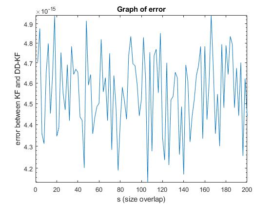
Figure 2: Graph of $error_{s}^{\Omega\times\Delta}$ versus the spatial overlap $s$ while time overlap is fixed to $s_{1,2}=1$.

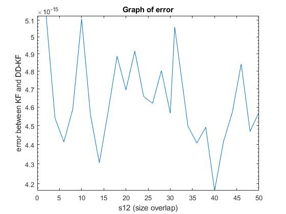
(a)

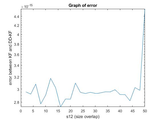
(b)

Figure 3: Behaviour of $error_{s_{1,2}}^{\Omega\times\Delta_{1}}$ and $error_{s_{1,2}}^{\Omega\times\Delta_{2}}$ versus the size of time overlap $s_{1,2}$ while the size of spatial overlap is $s=200$.

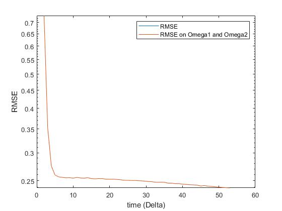
Figure 4: Behaviour of $RMSE_{k}^{\Omega_{1}\cup\Omega_{2}}$ and $RMSE_{k}^{\Omega}$ versus time.

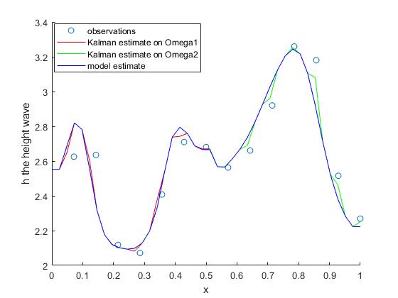
(a)

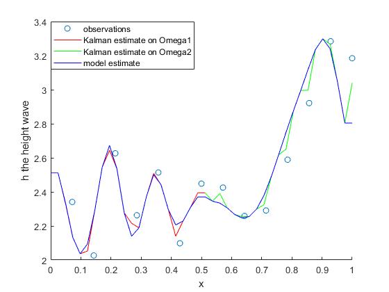
(b)

Figure 5: SWE solution and its DD-KF estimate.

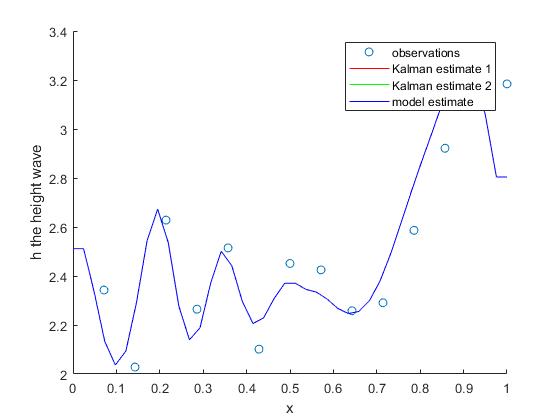
(a)

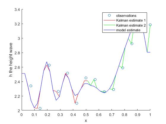
(b)

Figure 6: SWE solution and DD-KF estimates for different choices of $\sigma_{m}^{2}$ and $\sigma_{0}^{2}$.

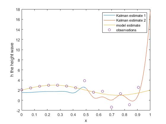
(a)

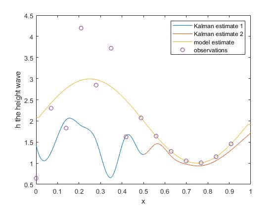
(b)

Figure 7: SWE solution and DD-KF estimates for different errors $v_{10}^{1}$, $v_{10}^{2}$ and variances observations $\sigma_{1,0}^{2}$ and $\sigma_{2,0}^{2}$ in $\Omega_{1}$ and $\Omega_{2}$, respectively. In order to point out the capability of DD-KF to deal with the presence of different observation errors, we show results obtained considering two different values of observations errors in $\Omega_{1}$ and $\Omega_{2}$, i.e. $v_{k}=[v_{k}^{1}v_{k}^{2}]$, respectively. Figure 7 (a) confirms the effect of the variance observations $\sigma_{2,0}^{2}=4.28\times 10^{0}$ on DD-KF estimate $\widehat{x}_{k}[1]^{\Omega\times\Delta}$ in $\Omega_{2}$; similarly, it occurs in $\Omega_{1}$ when $\sigma_{1,0}^{2}=1.04\times 10^{0}$, as Figure 7 (b) shows. As a consequence DD-KF method gives more confidence to model state than to the observations in $\Omega_{2}$ (a) or in $\Omega_{1}$ (b), depending on the variance observations.

6 Concluding remarks and future works

We have presented the mathematical framework which makes it possible using KF in any application involving real time state estimation. Borrowing Schwarz DD and PinT methods from PDEs, the framework properly combines KF localization and model reduction in space and time, fully revisited in a linear algebra settings. DD-KF framework makes it natural to switch from a full scale solver to a model order reduction solver for solution of subproblems for which no relevant low-dimensional reduced space should be constructed. Leveraging Schwarz and PinT methods consistency constraints for PDEs-based models, the framework iteratively adjust local solutions by adding the contribution of adjacent subdomains to the local filter, along overlapping regions. We derived and discussed main features of DD-KF framework using SWEs which are commonly used for monitoring and forecasting the water flow in rivers and open channels. Nevertheless, this framework has application on the plentiful literature of PDE-based state estimation real-world problems. As DD-KF is intended to give the same solution of KF experiments are exclusively aimed to validate DD-KF w.r.t. KF. Comparison against other KF methods which are approximations of KF, such as EnKF, are out of focus of the present work. Rather we note that the underlying idea of DD-KF could be applied to EnKF by changing the filter, as it is performed in DD-KF. Specifically, in order to enforce the matching of local solutions on adjacent regions, local problems should be slightly modified by adding the smoothness-regularization constraint to the correction phase on local solutions; such term keeps track of contributions of adjacent domains to ensembles regions. The same modification should be done on the covariance matrices.
This work makes possible numerous extensions. Among them, it makes it possible to apply deep-learning techniques to develop consistency constraints which will ensure that the solutions are physically meaningful even at the boundary of the small domains in the output of the local models deeplearning4; Hahnel; deeplearning3. Another possible extension could be the employment of a dynamic load balancing scheme based on adaptive and dynamic redefining of initial decomposition arxivPPAM2019; DyDD. Specifically, in order to optimally choose the domain decomposition configuration, the partitioning into subdomains must satisfy certain conditions. First the computational load assigned to subdomains must be equally distributed. Good quality partitioning also requires the volume of communication during calculation to be kept at its minimum. In arxivPPAM2019; DyDD the authors employed a dynamic load balancing scheme based on adaptive and dynamic redefining of initial decomposition, aimed to balance load between processors according to data location. In particular, the authors focused on the introduction of a dynamic redefining of initial DD in order to deal with problems where the observations are non uniformly distributed and general sparse. This is a quite common issue in DA. More generally, one would consider DD framework in multi-physics and multi-resolution applications, by employing adaptive and dynamic DD depending on the requirements of the application. Overall, the employment of the framework in high performance computing state estimation systems such as on board satellite navigation systems or autonomous vehicle tracking with GPS seems to be a fruitful research area.

7 Data Availability

The Matlab code used for the numerical simulations is available from the corresponding author upon request.

8 APPENDIX

In this section, with the aim of allowing the replicability of experimental results, we describe the the whole detailed derivation of DD-KF method on SWEs.

8.1 Preliminaries on DD

Definition (reduction of matrices): Let $B=[B^{1}\ B^{2}\ \ldots\ B^{n}]\in\mathbb{R}^{m\times n}$ be a matrix with $m,n\geq 1$ and $B^{j}$ the $j-th$ column of $B$ and $I_{j}=\{1,\ldots,j\}$ and $I_{i,j}=\{i,\ldots,j\}$ for $i=1,\ldots,n-1$ and $j=2,\ldots,n$. The reduction of $B$ to the set $I_{j}$ is:

$$|_{I_{j}}:\ B\in\mathbb{R}^{m\times n}\rightarrow\ B|_{I_{j}}=[B^{1}\ B^{2}\ \ldots\ B^{j}]\in\mathbb{R}^{m\times j},\quad\textit{ $j=2,\ldots,n$},$$ (68)

and to $I_{i,j}$

$${l}|_{I_{i,j}}:\ B\in\mathbb{R}^{m\times n}\rightarrow\ B|_{I_{i,j}}=[B^{i}\ B^{i+1}\ \ldots\ B^{j}]\in\mathbb{R}^{m\times j-i},$$ (69)

$$\textit{ $i=1,\ldots,n-1$, $j=2,\ldots,n$},$$ (70)

where $B|_{I_{j}}$ and $B|_{I_{i,j}}$ denote the reductions of $B$ to $I_{j}$ and $I_{i,j}$, respectively.
Definition (Extension of vectors): Let $w=[w_{t}\ w_{t+1}\ \ldots\ w_{n}]^{T}\in\mathbb{R}^{s}$ be a vector with $t\geq 1$, $n>1$, $s=n-t$. The extension of $w$ to $I_{r}$ where $r>n$ is:

$$EO_{I_{r}}:\ w\in\mathbb{R}^{s}\rightarrow\ EO_{I_{r}}(w)=[\bar{w}_{1}\ \bar{w}_{2}\ \ldots\ \bar{w}_{r}]^{T}\in\mathbb{R}^{r},$$ (71)

where, for $i=1,\ldots,r$, it is:

$$\bar{w}_{i}=\left\{\begin{array}[]{ll}w_{i}&\textit{if $t\leq i\leq n$}\\ 0&\textit{if $i>n$ and $i<t$ \quad.}\\ \end{array}\right.$$ (72)

8.2 DD-KF vs KF Performance Analysis

In order to quantify the benefit of the decomposition, i.e., how much the time complexity of the KF algorithm may be reduced with respect to the DD–KF based algorithm we use the so called scale-up factor introduced in CAI.

Definition 2

(Scale-up factor) Let $N_{p}\in\mathbb{N}$ be the problem size and $N_{sub}\geq 2$ the number of subdomains. Let $T_{KF}(N_{p})$ and $T_{DD-KF}(N_{sub})$ be time complexity of KF algorithm and DD-KF algorithm respectively. We introduce the scale-up factor:

$$Sc^{f}_{N_{sub},1}(N_{p})=\frac{T_{KF}(N_{p})}{N_{sub}\cdot T_{DD-KF}(N_{sub})}.$$ (73)

Following result allows us to analyze the behaviour of the scale up factor.

Proposition 1

Let $r\equiv N_{p}/N_{sub}$. Then it holds that

$$Sc^{f}_{N_{sub},1}(N_{p})=\alpha(N_{p},N_{sub})N_{sub}^{2}$$

where

$$\alpha(N_{p},N_{sub})=\frac{a_{3}+a_{2}\frac{1}{N_{p}}+a_{1}\frac{1}{N_{p}^{2}}+a_{0}\frac{1}{N_{p}^{3}}}{b_{3}+b_{2}\frac{1}{r}+b_{1}\frac{1}{r^{2}}+b_{0}\frac{1}{r^{3}}}.$$ (74)

Proof

We let $T_{KF}(N_{p})=p_{1}(N_{p})$ and $T_{DD-KF}(r)=p_{2}(r)$ where $p_{1}$ and $p_{2}$ are polynomials of degree less than or equal 3 i.e. $p_{1},p_{2}\in\Pi_{3}$:

$$\begin{array}[]{ll}T_{KF}(N_{p})=a_{3}N_{p}^{3}+a_{2}N_{p}^{2}+a_{1}N_{p}+a_{0}\\ T_{DD-KF}(r)=b_{3}r^{3}+b_{2}r^{2}+b_{1}r+b_{0}\end{array}.$$ (75)

It holds

$$\begin{array}[]{ll}Sc^{f}_{N_{sub},1}(m,N_{p})&=\frac{a_{3}N_{p}^{3}+a_{2}N_{p}^{2}+a_{1}N_{p}+a_{0}}{N_{sub}(b_{3}r^{3}+b_{2}r^{2}+b_{1}r+b_{0})}\cdot r^{3}\cdot\frac{1}{r^{3}}=\frac{a_{3}N_{sub}^{3}+a_{2}\frac{n_{sub}^{3}}{N_{p}}+a_{1}\frac{N_{sub}^{3}}{N_{p}^{2}}+a_{0}\frac{N_{sub}^{3}}{N_{p}^{3}}}{N_{sub}(b_{3}+b_{2}\frac{1}{r}+b_{1}\frac{1}{r^{2}}+b_{0}\frac{1}{r^{3}})}\\ \\ &=\frac{N_{sub}^{3}\cdot(a_{3}+a_{2}\frac{1}{N_{p}}+a_{1}\frac{1}{N_{p}^{2}}+a_{0}\frac{1}{N_{p}^{3}})}{N_{sub}(b_{3}+b_{2}\frac{1}{r}+b_{1}\frac{1}{r^{2}}+b_{0}\frac{1}{r^{3}})}=\frac{a_{3}+a_{2}\frac{1}{N_{p}}+a_{1}\frac{1}{N_{p}^{2}}+a_{0}\frac{1}{N_{p}^{3}}}{b_{3}+b_{2}\frac{1}{r}+b_{1}\frac{1}{r^{2}}+b_{0}\frac{1}{r^{3}}}\cdot N_{sub}^{2}\end{array}$$ (76)

and

$$Sc^{f}_{N_{sub},1}(N_{p})=\alpha(N_{p},N_{sub})N_{sub}^{2}$$

where

$$\alpha(N_{p},N_{sub})=\frac{a_{3}+a_{2}\frac{1}{N_{p}}+a_{1}\frac{1}{N_{p}^{2}}+a_{0}\frac{1}{N_{p}^{3}}}{b_{3}+b_{2}\frac{1}{r}+b_{1}\frac{1}{r^{2}}+b_{0}\frac{1}{r^{3}}}.$$ (77)

Recalling that $r=\frac{N_{p}}{N_{sub}}$ and $Sc^{f}_{N_{sub},1}(N_{p})=\alpha(N_{p},N_{sub})N_{sub}^{2}$, this result says that the performance gain of DD-KF algorithm in terms of reduction of time complexity, scales as the number of subdomains $N_{sub}$ squared, where the scaling factor depends on $\alpha(N_{p},N_{sub})$, that is, on the time complexity of the algorithms.

8.3 SWE setup

Neglecting the Coriolis force and frictional forces and assuming unit width, SWEs are:

$$\left\{\begin{array}[]{ll}\frac{\partial h}{\partial t}+\frac{\partial vh}{\partial{x}}=0\\ \frac{\partial vh}{\partial t}+\frac{\partial(v^{2}h+\frac{1}{2}gh^{2})}{\partial{x}}=0\end{array}\right.$$ (78)

where the independent variables ${x}$ and $t$ make up the spatial dimension and time. The dependent variables are $h$, which is the height with respect to the surface and $v$, i.e. the horizontal velocity, while $g$ is the gravitational acceleration.
In order to write SWEs in a compact form, we introduce the vectors

$$\textbf{x}:=\left[\begin{array}[]{ll}h\\ vh\end{array}\right]\quad f(\textbf{x}):=\left[\begin{array}[]{ll}vh\\ v^{2}h+\frac{1}{2}gh^{2}\end{array}\right],$$ (79)

the SWEs can be rewritten as follows

$$\frac{\partial\textbf{x}}{\partial t}+\frac{\partial f(\textbf{x)}}{\partial{x}}=0.$$ (80)

The initial boundary problem for the SWEs is

$$\left\{\begin{array}[]{lllll}\textbf{x}(t+\Delta t,x)=\mathcal{M}_{t,t+\Delta t}(\textbf{x}(t,x))\quad\forall t,t+\Delta t\in[0,1.5]\\ \textbf{x}(0,x):=\left[\begin{array}[]{ll}h(0,x)\\ h(0,x)v(0,x)\end{array}\right]=\left[\begin{array}[]{ll}2+\sin(2\pi x)\\ 0\end{array}\right]\quad\forall x\in\Omega\end{array}\right.$$ (81)

with the following reflective boundary conditions on $v$ and free boundary conditions on $h$

$$\textbf{x}(t,0):=\left[\begin{array}[]{ll}h(t,x_{1})\\ -h(t,x_{1})v(t,x_{1})\end{array}\right]\quad\textbf{x}(t,x_{n_{x}-1}):=\left[\begin{array}[]{ll}h(t,x_{n_{x}-2})\\ -h(t,x_{n_{x}-2})v(t,x_{n_{x}-2})\end{array}\right]\quad\forall t\in\Delta$$ (82)

where

$$\mathcal{M}_{t,t+\Delta t}(\textbf{x}(t,x)):=\textbf{x}(t,x)-\int_{t}^{t+\Delta t}\frac{\partial f(\textbf{x})}{\partial x}ds.$$ (83)

We note that $\mathcal{M}_{t,t+\Delta t}(\textbf{x}(t,x))$ should include Coriolis forces and also frictional forces, if they are present in the SWEs; in particular, as these quantities show off as the right hand side of (80), they will be also included in the right hand side of (83) as additive terms under the integral.
The state of the system at each time $t_{k+1}\in\Delta$, $k=0,1,\ldots,nt-2$ is:

$$\textbf{x}(t_{k+1})\equiv\textbf{x}_{k+1}:=\left[\begin{array}[]{lll}x[1]_{k+1}\\ x[2]_{k+1}\end{array}\right]\in\mathbb{R}^{2(n_{x}-2)}$$ (84)

where

$$\begin{array}[]{lll}x[1]_{k+1}&\>=\{x[1](t_{k+1},x_{i})\}_{i=1,\ldots,n_{x}-1}&:=\{h(t_{k+1},x_{i})\}_{i=1,\ldots,n_{x}-1}\in\mathbb{R}^{(n_{x}-2)}\\ x[2]_{k+1}&:=\{x[2](t_{k+1},x_{i})\}_{i=1,\ldots,n_{x}-1}&:=\{v(t_{k+1},x_{i})h(t_{k+1},x_{i})\}_{i=1,\ldots,n_{x}-1}\in\mathbb{R}^{(n_{x}-2)}\end{array}.$$ (85)

From Lax-Wendroff scheme LeVeque, we obtain the following discrete formulation of the SWEs

$$\textbf{x}_{k+1}=M_{k,k+1}\textbf{x}_{k}+b_{k}+w_{k}$$ (86)

where

$$M_{k,k+1}=\left[\begin{array}[]{lllllllllllll}M[1]_{k,k+1}\ \ O_{n_{x}-2}\\ M[2,1]_{k,k+1}\ \ M[2]_{k,k+1}\end{array}\right]\in\mathbb{R}^{2(n_{x}-2)\times 2(n_{x}-2)}$$ (87)

with $O_{n_{x}-2}\in\mathbb{R}^{n_{x}-2\times n_{x}-2}$ the null matrix and $M[1]_{k,k+1}\in\mathbb{R}^{(n_{x}-2)\times(n_{x}-2)}$, $M[2,1]_{k,k+1}\in\mathbb{R}^{(n_{x}-2)\times(n_{x}-2)}$, $M[2]_{k,k+1}\in\mathbb{R}^{(n_{x}-2)\times(n_{x}-2)}$ the following tridiagonal matrices

$$M[1]_{k,k+1}=\left[\begin{array}[]{lllllllllllll}\psi_{1}^{k}&\eta_{2}^{k}&&&\\ -\eta_{1}^{k}&\psi_{2}^{k}&\eta_{3}^{k}&&\\ &\ddots&\ddots&\ddots\\ &&-\eta_{n_{x}-4}^{k}&\psi_{n_{x}-3}^{k}&\eta_{n_{x}-2}^{k}\\ &&&-\eta_{n_{x}-3}^{k}&\psi_{n_{x}-2}^{k}\end{array}\right]$$ (88)

$$M[2,1]_{k,k+1}=\left[\begin{array}[]{lllllllllllll}0&\chi_{2}^{k}&&&\\ -\chi_{1}^{k}&0&\chi_{3}^{k}&&\\ &\ddots&\ddots&\ddots\\ &&-\chi_{n_{x}-4}^{k}&0&\chi_{n_{x}-2}^{k}\\ &&&-\chi_{n_{x}-3}^{k}&0\end{array}\right]$$ (89)

$$M[2]_{k,k+1}=\left[\begin{array}[]{lllllllllllll}\phi_{1}^{k}&\xi_{2}^{k}&&&\\ -\xi_{1}^{k}&\phi_{2}^{k}&\xi_{3}^{k}&&\\ &\ddots&\ddots&\ddots\\ &&-\xi_{n_{x}-4}^{k}&\phi_{n_{x}-3}^{k}&\xi_{n_{x}-2}^{k}\\ &&&-\xi_{n_{x}-3}^{k}&\phi_{n_{x}-2}^{k}\end{array}\right]$$ (90)

and the vector $b\in\mathbb{R}^{2(n_{x}-2)}$

$$b_{k}:=\left[\begin{array}[]{ll}b[1]_{k}\\ b[2]_{k}\end{array}\right]\in\mathbb{R}^{2(n_{x}-2)}$$ (91)

with

$$b[1]_{k}:=\left[\begin{array}[]{ll}\eta_{0}^{k}h_{0}^{k}\\ 0\\ \vdots\\ 0\\ \eta_{n_{x}-1}^{k}h_{n_{x}-1}^{k}\end{array}\right]\in\mathbb{R}^{n_{x}-2}\quad b[2]_{k}:=\left[\begin{array}[]{ll}\xi_{0}^{k}v_{0}^{k}h_{0}^{k}-\chi_{0}^{k}h_{0}^{k}\\ 0\\ \vdots\\ 0\\ \xi_{n_{x}-1}^{k}h_{n_{x}-1}^{k}+\xi_{n_{x}-1}^{k}v_{n_{x}-1}^{k}h_{n_{x}-1}^{k}\end{array}\right]\in\mathbb{R}^{n_{x}-2}$$ (92)

where

$$\begin{array}[]{lllllll}\eta_{i}^{k}&:=\frac{\alpha}{2}[v_{i}^{k}+\alpha((v_{i}^{k})^{2}+\frac{1}{2}gh_{i}^{k})]&\quad\psi_{i}^{k}&:=1-4\alpha^{2}((v_{i}^{k})^{2}+\frac{1}{2}gh_{i}^{k})\\ \xi_{i}^{k}&:=\frac{\alpha}{2}[\alpha+v_{i}^{k}]&\quad\phi_{i}^{k}&:=\left(1+4\alpha^{2}\right)\end{array}$$

$$\chi_{i}^{k}:=\frac{1}{2}gh_{i}^{k}$$

with $\alpha:=\frac{\Delta t}{2\Delta x}$ and $h_{i}^{k}:=h(t_{k},x_{i})$, $v_{i}^{k}:=v(t_{k},x_{i})$.
We note that the discrete model in (86) can be rewritten as follows

$$\begin{array}[]{ll}x[1]_{k+1}={M}[1]_{k,k+1}x[1]_{k}+b[1]_{k}\\ x[2]_{k+1}={M}[2]_{k,k+1}x[2]_{k}+\tilde{b}[2]_{k}\end{array}$$ (93)

with

$$\tilde{b}[2]_{k}:={b}[2]-M[2,1]_{k,k+1}x[1]_{k}.$$ (94)

In particular, if we define

$$S:=\max\left(|v-\sqrt{gh}|,|v+\sqrt{gh}|\right),$$ (95)

the stability condition of Lax-Wendroff is

$$S\cdot\frac{\Delta t}{\Delta x}\leq 1,$$ (96)

for the condition (96) to be satisfied, at each iteration $k=0,1,\ldots,nt$ we choose: $\Delta t=0.8\cdot\frac{\Delta x}{S}$.

1. Decomposition Step.

   • Decomposition of $\Omega$ into two subdomains with overlap region:

     $$\begin{array}[]{ll}\Omega_{1}=[0,x_{n_{1}}]\quad\textrm{with $D_{n_{1}+1}(\Omega_{1})=\{x_{i}\}_{i=0,1,\ldots,n_{1}}$ }\\ \Omega_{2}=[x_{n_{1}-s+1},1]\quad\textrm{with $D_{n_{2}+1}({\Omega}_{2})=\{x_{i}\}_{i=n_{1},\ldots,n-1}$}\end{array}$$ (97)

   • Decomposition of $\Delta$ into two subsets with overlap region:

     $$\begin{array}[]{ll}\Delta_{1}=[0,t_{s_{1}-1}]\quad\textrm{with $D_{s_{1}}(\Delta_{1})=\{t_{k}\}_{k=0,\ldots,s_{1}-1}$}\\ \Delta_{2}=[t_{s_{1}-s_{1,2}+1},1.5]\quad\textrm{with $D_{s_{2}}(\Delta_{2})=\{t_{k}\}_{k=s_{1}-s_{1,2}+1,\ldots,nt-1}$}.\end{array}$$ (98)

2. Local initial conditions on $\Delta_{1}$ and $\Delta_{2}$:

   $$\begin{array}[]{ll}x[1]_{0}^{\Delta_{1}}=h(0,x)=:x[1]_{0}^{\Delta_{0}}\\ x[2]_{0}^{\Delta_{1}}=h(0,x)v(0,x)=:x[2]_{0}^{\Delta_{0}}\end{array}\quad\begin{array}[]{ll}x[1]_{{s_{1}-1}}^{\Delta_{2}}=x[1]_{{s_{1}-1}}^{\Delta_{1}}\\ x[2]_{{s_{1}-1}}^{\Delta_{2}}=x[2]_{{s_{1}-1}}^{\Delta_{1}}\end{array}.$$ (99)

3. Model decomposition in (93).
   Decomposition of matrices $M[1]_{k+1}\in\mathbb{R}^{n_{x}-2}$ at each step $k=0,1,\ldots,nt-2$

   $$M[1]_{k,k+1}^{1}:=M[1]_{k,k+1}|_{I_{1}\times I_{1}}=\left[\begin{array}[]{lllllllllllll}\psi_{1}^{k}&\eta_{2}^{k}&&&\\ -\eta_{1}^{k}&\psi_{2}^{k}&\eta_{3}^{k}&&\\ &\ddots&\ddots&\ddots\\ &&-\eta_{n_{1}-2}^{k}&\psi_{n_{1}-1}^{k}&\eta_{n_{1}}^{k}\\ &&&-\eta_{n_{1}-1}^{k}&\psi_{n_{1}}^{k}\end{array}\right]\in\mathbb{R}^{n_{1}\times n_{1}}$$ (100)

   $$M[1]_{k,k+1}^{1,2}:=M[1]_{k,k+1}|_{I_{1}\times I_{2}}=\left[\begin{array}[]{lllllllllllll}0&\cdots&\cdots&\cdots&0&\cdots&0\\ 0&\cdots&\cdots&\cdots&0&\cdots&0\\ \vdots&&&&&&\vdots\\ &&&&\\ 0&\cdots&0&\eta_{n_{1}+1}^{k}&0&\cdots&0\\ \end{array}\right]\in\mathbb{R}^{n_{1}\times n_{2}}$$ (101)

   $$M[1]_{k,k+1}^{2,1}:=M[1]_{k,k+1}|_{I_{1}\times I_{2}}=\left[\begin{array}[]{lllllllllllll}0&\cdots&0&0&\eta_{n_{1}}^{k}&0&\cdots&0\\ 0&\cdots&0&\cdots&0&0&\cdots&0\\ \vdots&&&&\vdots&\vdots&&\vdots\\ &&&&\\ 0&\cdots&0&\cdots&0&0&\cdots&0\\ \end{array}\right]\in\mathbb{R}^{n_{2}\times n_{1}}$$ (102)

   $$M[1]_{k,k+1}^{2}:=M[1]_{k,k+1}|_{I_{2}\times I_{2}}=\left[\begin{array}[]{lllllllllllll}\psi_{n_{1}}^{k}&\eta_{n_{1}+1}^{k}&&&\\ -\eta_{n_{1}}^{k}&\psi_{n_{1}+1}^{k}&\eta_{n_{1}+2}^{k}&&\\ &\ddots&\ddots&\ddots\\ &&-\eta_{n_{x}-4}^{k}&\psi_{n_{x}-3}^{k}&\eta_{n_{x}-2}^{k}\\ &&&-\eta_{n_{1}-3}^{k}&\psi_{n_{x}-2}^{k}\end{array}\right]\in\mathbb{R}^{n_{2}\times n_{2}}.$$ (103)

   We proceed in the same way to get the decomposition of matrix $M[2]_{k,k+1}\in\mathbb{R}^{n_{x}-2\times n_{x}-2}$ in (93) into $M[2]_{k,k+1}^{1}\in\mathbb{R}^{n_{1}\times n_{1}}$, $M[2]_{k,k+1}^{1,2}\in\mathbb{R}^{n_{1}\times n_{2}}$, $M[2]_{k,k+1}^{2,1}\in\mathbb{R}^{n_{2}\times n_{1}}$ and $M[2]_{k,k+1}^{2}\in\mathbb{R}^{n_{2}\times n_{2}}$.

4. Decomposition of $H_{k+1}\in\mathbb{R}^{m\times(n_{x}-2)}$ into $H_{k+1}^{1}\in\mathbb{R}^{m\times n_{1}}$ and $H_{k+1}^{2}\in\mathbb{R}^{m\times n_{2}}$ as in (30).

8.4 DD-KF method.

1. For $j=1,2$ and $k=\bar{s}_{j-1}+1,\ldots,\bar{s}_{j-1}+s_{j}$, we apply DD-KF method on $\Delta_{1}$ and $\Delta_{2}$ by considering the following matrices:

   $$\begin{array}[]{llllll}M_{1}[i]&\equiv M[i]_{k,k+1}^{1}&\quad M_{1,2}[i]&\equiv M[i]_{k,k+1}^{1,2}\\ M_{2}[i]&\equiv M[i]_{k,k+1}^{2}&\quad M_{2,1}[i]&\equiv M[i]_{k,k+1}^{2,1}\\ P_{1}&=O_{n_{1}\times n_{1}}&\quad P_{2}&=O_{n_{2}\times n_{2}}\\ P_{1,2}&=O_{n_{1}\times n_{2}}&\quad P_{2,1}&=O_{n_{2}\times n_{1}}\end{array}.$$ (104)

   In particular, we note:

   $$M_{1,2}[i]\equiv\left[\begin{array}[]{lll}O&M_{1,3}[i]\\ O&M_{2,3}[i]\end{array}\right]\quad M_{2,1}[i]\equiv\left[\begin{array}[]{lll}\tilde{M}_{1,2}[i]&O\\ \tilde{M}_{2,1}[i]&O\end{array}\right].$$ (105)

2. Send and receive boundary conditions from adjacent domains and compute the vectors:

   $$b_{1,k}[i]=\left[\begin{array}[]{lll}M_{1,3}[i]\\ M_{2,3}[i]\end{array}\right]\widehat{x}_{2,k}[i]|_{\Gamma_{1}}\quad b_{2,k}[i]=\left[\begin{array}[]{lll}\tilde{M}_{1,2}[i]\\ \tilde{M}_{2,1}[i]\end{array}\right]\widehat{x}_{1,k}[i]|_{\Gamma_{2}}.$$ (106)

3. For $j=1,2$ and $k=\bar{s}_{j-1}+1,\ldots,\bar{s}_{j-1}+s_{j}$, compute the predicted state estimates $x_{1,k+1}[i]\in\mathbb{R}^{n_{1}}$ and $x_{2,k+1}[i]\in\mathbb{R}^{n_{2}}$ for $i=1,2$, as follows:

   $$\begin{array}[]{ll}x_{1,k+1}[i]=M_{1}[i]\widehat{x}[i]_{k}^{\Delta_{j-1}}|_{I_{1}}+\bar{b}[i]_{k}|_{I_{1}}+b_{1,k}\\ x_{2,k+1}[i]=M_{2}[i]\widehat{x}[i]_{\bar{s}_{j}}^{\Delta_{j-1}}|_{I_{2}}+\bar{b}[i]|_{I_{2}}+b_{2,k}\end{array},$$ (107)

   with

   $$\bar{b}[i]_{k}=\left\{\begin{array}[]{lll}b[1]_{k}&\textrm{in (\ref{b[1]})}&\textrm{if $i=1$}\\ \tilde{b}[2]_{k}&\textrm{in (\ref{tilde_b[2]})}&\textrm{if $i=2$}\end{array}.\right.$$ (108)

4. For $j=1,2$ and $k=\bar{s}_{j-1},\ldots,\bar{s}_{j-1}+s_{j}-1$, compute DD-KF estimates as in (51) on $\Delta_{j}$ i.e. $\widehat{x}_{1,k+1}^{\Delta_{j}}[i]\equiv\widehat{x}[i]_{1,k+1}\in\mathbb{R}^{n_{1}}$ and $\widehat{x}_{2,k+1}^{\Delta_{j}}[i]\equiv\widehat{x}[i]_{2,k+1}\in\mathbb{R}^{n_{2}}$. In particular, in the time interval $\Delta_{j}$, by considering the boundary conditions in (82), DD-KF estimates on $\Omega_{1}$ and $\Omega_{2}$ are

   $$\begin{array}[]{ll}\widehat{x}_{k+1}^{\Omega_{1}\times\Delta_{j}}[i]&:=\left[\begin{array}[]{ll}{x}(t_{k+1},0)[i]\\ \widehat{x}_{1,k+1}^{\Delta_{j}}[i]\\ \widehat{x}_{2,k+1}^{\Delta_{j}}[i](1)\end{array}\right]\in\mathbb{R}^{n_{1}+1}\\ \widehat{x}_{k+1}^{\Omega_{2}\times\Delta_{j}}[i]&:=\left[\begin{array}[]{ll}\widehat{x}_{1,k+1}^{\Delta_{j}}[i](n_{1}-s)\\ \widehat{x}_{2,k+1}^{\Delta_{j}}[i]\\ {x}(t_{k+1},x_{n_{x}-1})[i]\end{array}\right]\in\mathbb{R}^{n_{2}+1}\end{array}$$ (109)

   where $\widehat{x}_{r,k+1}^{\Delta_{j}}[i](1)$, $\widehat{x}_{r,k+1}^{\Delta_{j}}[i](n_{1}-s)$ are the first and the $n_{1}-s$ components of $\widehat{x}_{r,k+1}^{\Delta_{j}}[i]$, $r=1,2$. We refer to

   $$\widehat{x}_{k+1}[i]^{\Omega\times\Delta_{j}}:=\left[\begin{array}[]{ll}\widehat{x}_{k+1}^{\Omega_{1}\times\Delta_{j}}[i]\\ \widehat{x}_{k+1}^{\Omega_{1,2}\times\Delta_{j}}[i]\\ \widehat{x}_{k+1}^{\Omega_{2}\times\Delta_{j}}[i]\end{array}\right]\in\mathbb{R}^{n_{x}}$$ (110)

   as the estimate of the wave height and velocity (if $i=1,2$ respectively) obtained by applied the DD-KF method on $\Omega$, where on the spatial overlap $\Omega_{1,2}$, we have considered the arithmetic mean between DD-KF estimates i.e.

   $$\widehat{x}_{k+1}^{\Omega_{1,2}\times\Delta_{j}}[i]:=\left[\begin{array}[]{ll}\frac{\widehat{x}_{k+1}^{\Omega_{1}\times\Delta_{j}}[i]|_{I_{1,2}}+\widehat{x}_{k+1}^{\Omega_{2}\times\Delta_{j}}[i]|_{I_{1,2}}}{2}\end{array}\right]$$ (111)

   with $I_{1,2}$ the index set defined in (17).

Table 2: DD-KF to SWEs

procedure DD-KF-SWE
Domain Decomposition Step: Decomposition of $\Omega$ and of $\Delta$
SWE Model setup as in (78) – (95)
Define Local initial conditions on $\Delta_{1}$ and $\Delta_{2}$ as in (99)
Reduction of $M_{k,k+1}$ in (93)
Reduction of $H_{l+1}\in\mathbb{R}^{n_{obs}\times(n_{x}-2)}$ as in (30).
for $k=1,2$
for $l=\bar{s}_{k-1}+1,\ldots,\bar{s}_{k-1}+s_{k}$, as in (20) % apply DD-KF method on $\Delta_{k}$
Send and receive boundary conditions from adjacent domains as in (106 )
Compute

$$b_{1,l}[i]=\left[\begin{array}[]{lll}M_{1,3}[i]\\ M_{2,3}[i]\end{array}\right]\widehat{x}_{2,l}[i]|_{\Gamma_{1}}\quad b_{2,l}[i]=\left[\begin{array}[]{lll}\tilde{M}_{1,2}[i]\\ \tilde{M}_{2,1}[i]\end{array}\right]\widehat{x}_{1,l}[i]|_{\Gamma_{2}}.$$

Compute the predicted state estimates $x_{1,l+1}[i]\in\mathbb{R}^{n_{1}}$ and $x_{2,l+1}[i]\in\mathbb{R}^{n_{2}}$

$$\begin{array}[]{ll}x_{1,l+1}[i]=M_{1}[i]\widehat{x}[i]_{l}^{\Delta_{k-1}}|_{I_{1}}+\bar{b}[i]_{l}|_{I_{1}}+b_{1,l}\\ x_{2,l+1}[i]=M_{2}[i]\widehat{x}[i]_{\bar{s}_{k}}^{\Delta_{k-1}}|_{I_{2}}+\bar{b}[i]|_{I_{2}}+b_{2,l}\end{array},$$

with

$$\bar{b}[i]_{l}=\left\{\begin{array}[]{lll}b[1]_{l}&\textrm{in (\ref{b[1]})}&\textrm{if $i=1$}\\ \tilde{b}[2]_{l}&\textrm{in (\ref{tilde_b[2]})}&\textrm{if $i=2$}\end{array}.\right.$$

Compute DD-KF estimates as in (51) on $\Omega_{i}\times\Delta_{k}$

$$\begin{array}[]{ll}\widehat{x}_{l+1}^{\Omega_{1}\times\Delta_{k}}[i]&:=\left[\begin{array}[]{ll}{x}(t_{l+1},0)[i]\\ \widehat{x}_{1,l+1}^{\Delta_{k}}[i]\\ \widehat{x}_{2,l+1}^{\Delta_{k}}[i](1)\end{array}\right]\in\mathbb{R}^{n_{1}+1}\\ \widehat{x}_{l+1}^{\Omega_{2}\times\Delta_{k}}[i]&:=\left[\begin{array}[]{ll}\widehat{x}_{1,l+1}^{\Delta_{k}}[i](n_{1}-\delta/2)\\ \widehat{x}_{2,l+1}^{\Delta_{k}}[i]\\ {x}(t_{l+1},x_{n_{x}-1})[i]\end{array}\right]\in\mathbb{R}^{n_{2}+1}\end{array}$$

Compute DD-KF estimate on $\Omega\times\Delta_{k}$

$$\widehat{x}_{l+1}[i]^{\Omega\times\Delta_{k}}:=\left[\begin{array}[]{ll}\widehat{x}_{l+1}^{\Omega_{1}\times\Delta_{k}}[i]\\ \widehat{x}_{l+1}^{\Omega_{1,2}\times\Delta_{k}}[i]\\ \widehat{x}_{l+1}^{\Omega_{2}\times\Delta_{k}}[i]\end{array}\right]\in\mathbb{R}^{n_{x}}$$

and

$$\widehat{x}_{l+1}^{\Omega_{1,2}\times\Delta_{k}}[i]:=\left[\begin{array}[]{ll}\frac{\widehat{x}_{l+1}^{\Omega_{1}\times\Delta_{k}}[i]|_{I_{1,2}}+\widehat{x}_{l+1}^{\Omega_{2}\times\Delta_{k}}[i]|_{I_{1,2}}}{2}\end{array}\right]$$

with $I_{1,2}$ defined in (17).
endprocedure