On the maximum black hole mass at solar metallicity

Abstract

Recently, models obtained with MESA and Genec detailed evolutionary codes indicated that black holes formed at solar metallicity ($Z=0.014$) may reach $35{\rm~{}M}_{\odot}$ or even higher masses. We perform a replication study to assess the validity of these results. We use MESA and Genec to calculate a suite of massive stellar models at solar metallicity. In our calculations we employ updated physics important for massive star evolution (moderate rotation, high overshooting, magnetic angular momentum transport). The key feature of our models is a new prescription for stellar winds for massive stars that updates significantly previous calculations. We find a maximum BH mass $M_{\rm BH,max}=28{\rm~{}M}_{\odot}$ at $Z=0.014$. The most massive BHs are predicted to form from stars with initial mass of $M_{\rm zams}\sim 40{\rm~{}M}_{\odot}$ and for stars with $M_{\rm zams}\gtrsim 200{\rm~{}M}_{\odot}$. The lower mass BHs found in our study mostly result from the updated wind mass loss prescriptions. While we acknowledge the inherent uncertainties in stellar evolution modelling, our study underscores the importance of employing the most up-to-date knowledge of key physics (e.g., stellar wind mass loss rates) in BH mass predictions.

1. Introduction

The LIGO/Virgo/KAGRA (LVK) collaboration has delivered summary of detections of compact object mergers in gravitational-waves in $3$ observing runs O1/O2/O3 (The LIGO Scientific Collaboration et al., 2023). The majority of these detections are black hole black hole (BH-BH) mergers. BHs are found in wide mass range $\sim 2.6-95{\rm~{}M}_{\odot}$. LVK inferred intrinsic an BH mass distribution for more massive BH in BH-BH mergers. The distribution decreases steeply with the primary BH mass and it shows two peaks at $\sim 8{\rm~{}M}_{\odot}$ and $\sim 35{\rm~{}M}_{\odot}$. Understanding such result is a complex task. The number of evolutionary channels may lead to the formation of BH-BH mergers (e.g.,  Mandel & Broekgaarden (2022)), and each channel has its own inherent uncertainties (e.g.,  Belczynski et al. (2022)). In many of the formation channels stars are the building blocks for BH-BH mergers. There is therefore the need for precise predictions from stellar evolution in regard to final state of massive stars at the time of core-collapse. Such predictions allow, among other things, to estimate stellar-origin BH masses. The BH mass is predicted to depend sensitively on metallicity (Belczynski et al., 2010b, a). Yet, a good starting point for such calculations is solar metallicity.

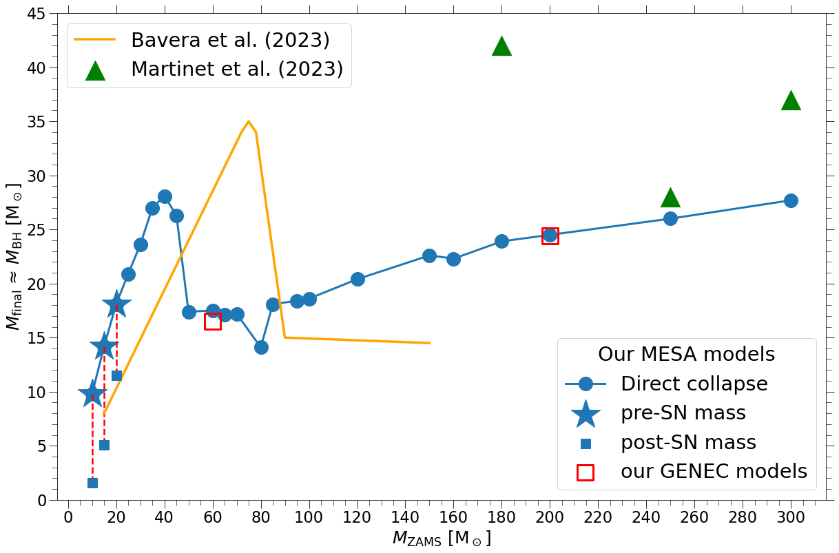
Recently, two studies offered new results in terms of final masses of massive stellar models. Final star mass may be taken as a proxy for BH mass (direct BH formation) or as an upper limit on BH mass (if there is a supernova explosion involved in BH formation). First,  Bavera et al. (2023a) performed stellar evolution of massive stars in the Zero-Age Main Sequence (ZAMS) star mass range $M_{\rm zams}=15-150{\rm~{}M}_{\odot}$ at $Z=0.014$ with the MESA evolutionary code. They found that BH mass increases from $M_{\rm BH}=3{\rm~{}M}_{\odot}$ at $M_{\rm zams}=15{\rm~{}M}_{\odot}$ to peak value at $M_{\rm BH}=35{\rm~{}M}_{\odot}$ at $M_{\rm zams}=75{\rm~{}M}_{\odot}$, and then BH mass rapidly decreases with initial mass to $M_{\rm BH}=15{\rm~{}M}_{\odot}$ at $M_{\rm zams}=100{\rm~{}M}_{\odot}$. They also found that for more massive stars ($M_{\rm zams}>100{\rm~{}M}_{\odot}$) BH mass does not change at remains more or less constant ($M_{\rm BH}=14{\rm~{}M}_{\odot}$). Second,  Martinet et al. (2023) provided models performed with the Genec (Geneva evolution code). We only pick the rotating models at $Z=0.014$ from this study for our comparison. These include $M_{\rm zams}=180,\ 250,\ 300{\rm~{}M}_{\odot}$. Final masses (end of C-burning) of these models are $M_{\rm final}=42,\ 28,\ 37{\rm~{}M}_{\odot}$. Additionally these models at final stage are WC/WO spectral subtype stars. For such final masses we may expect that they approximately correspond to BH masses. On one hand for such high final masses supernova models predict direct BH formation (Fryer et al., 2012a), on the other hand pulsational pair-instability supernovae are predicted to start removing mass for helium cores more massive than $\sim 35-40{\rm~{}M}_{\odot}$ (Woosley, 2017).

Both of the above calculations have employed “Dutch”-like wind mass loss prescriptions that are selections of wind models from various papers and and commonly used in detailed evolutionary calculations. However, recent years offered various detailed studies of massive stars and their mass loss through stellar winds (e.g., Krtička & Kubát (2017); Björklund et al. (2021); Gormaz-Matamala et al. (2023)). We take advantage of these new results to update our calculations. Additionally, in  Bavera et al. (2023a) only non-rotating models were used, and in Martinet et al. (2023) a rather modest overshooting was employed ($\alpha_{\rm ov}\sim 0.2$).

Here we propose an updated collection of wind-mass loss prescriptions that can be applied to all massive stars that are expected to form BHs. We also advocate for the use of rotating models to better represent the reality of stellar populations and the adoption of high overshooting values ($\alpha_{\rm ov}=0.5$) for all massive stars as showed by  Scott et al. (2021). We perform most of our models with our updated version of MESA, and we cross-check our MESA results with a couple of calculations performed with our Genec models. Both codes are made to run possibly the same physics (same winds, rotation, convection/overshooting, angular momentum transport).

Figure 1.— Adopted wind mass loss prescription for massive stars at solar metallicity (Z=0.014). See Sec. 2.1 for details.

2. Modelling

In our study we use two different detailed evolutionary codes, the version 23.05.1 of Modules for Experiments in Stellar Astrophysics (MESA Paxton et al., 2011, 2013, 2015, 2018, 2019; Jermyn et al., 2023), and Genec (Eggenberger et al., 2008) for stars at solar metallicity $Z=0.014$ (Asplund et al., 2009) within an initial mass range between $10$ and $300{\rm~{}M}_{\odot}$. We unified key input physics in both codes. We stop all our simulations at the depletion of carbon in the stellar core, since the timescale between the end of core C burning and the core-collapse is negligible in terms of star and core mass evolution (see e.g. Woosley et al. 2002) and would not therefore change the final estimates for BH masses.

2.1. Mass loss prescription

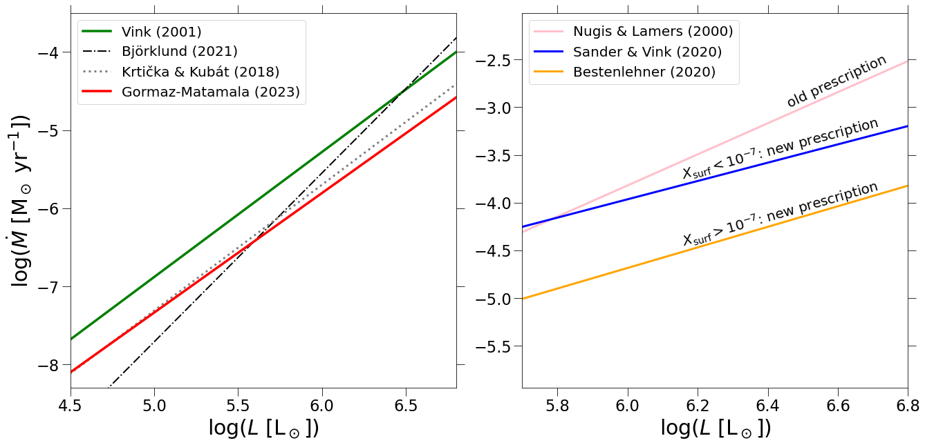
The theoretical calculation of wind mass loss rates ($\dot{M}$) depends on the physical properties of a star, and stellar winds change with the spectral type and evolutionary stage changes. In Figure 1 we show our adopted wind mass loss prescription. Our choices are motivated by recent work on various phases of wind mass loss for massive stars. Yet we use older prescriptions in parts of parameter space where no updates are available.

Figure 2.— Left: H-R diagram for selected MESA models. Colors correspond to various wind mass loss prescriptions used in our study. Note that stars with initial masses $M_{\rm zams}\lesssim 60{\rm~{}M}_{\odot}$ are subject to significant radial expansion, while more massive stars do not expand during evolution. Right: Fraction of ZAMS mass lost through given wind mass loss prescription (color coded as shown in the figure). Note that majority of mass loss for most massive stars ($M_{\rm zams}\gtrsim 60{\rm~{}M}_{\odot}$) is expected by H-rich thick winds and by H-poor thick winds (for which we use recent updated formulae).

Figure 3.— ZAMS mass — final star mass (end of C-burning) relation at solar metallicity $Z=0.014$. Our updated MESA models are shown with blue points (final mass of a star equals mass of a BH: no supernova) and blue stars (upper limit on mass of a BH, where blue squares show our estimates of NS/BH mass after supernova). Our two updated Genec models are shown with red squares. Predictions from both codes match. Our predicted maximum BH mass is $M_{\rm BH,max}=28{\rm~{}M}_{\odot}$ and is obtained for ZAMS mass $M_{\rm zams}\sim 40{\rm~{}M}_{\odot}$. High BH masses ($M_{\rm BH}\gtrsim 25{\rm~{}M}_{\odot}$) are also predicted for very massive stars $M_{\rm zams}\gtrsim 200{\rm~{}M}_{\odot}$. For comparison we also show models from  Bavera et al. (2023a) (yellow line) and from  Martinet et al. (2023) (green triangles): note that these models predict higher BH masses than our models.

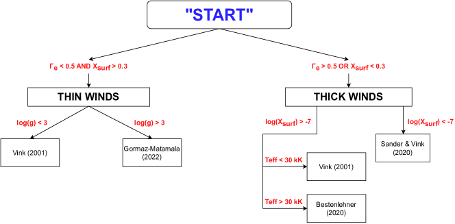
For the line-driven winds, which are the dominant winds for the mass range we are evaluating in this work, we make the division between optically thin and optically thick winds.

Optically thin winds models imply that the stellar radius is well defined (such as OBA-type stars), whereas optically thick wind implies that there is not a clear separation between the photosphere and the expanded atmosphere, such as in Wolf-Rayet (WR) stars. For stellar evolution models, this distinction is made when the star is hot and its mass fraction of surface hydrogen $X_{\rm surf}$ is below certain value, normally $X_{\rm surf}<0.3$ or $<0.4$ (Yusof et al., 2013; Köhler et al., 2015). However, very massive stars such as WNh develop thick winds in early stages of their evolution (Tehrani et al., 2019; Martins & Palacios, 2022) because of their proximity to the Eddington limit due to their extreme luminosity (Vink et al., 2011; Bestenlehner et al., 2014; Gräfener, 2021). For this reason, for stars with large hydrogen mass fraction at surface we set the transition from thin to thick winds when the Eddington factor $\Gamma_{\text{e}}$ reaches some $\Gamma_{\text{e,trans}}$. Studies analyzing the wind efficiency have found a smooth transition between thin and thick winds, without abrupt jumps in $\dot{M}$ (Vink & Gräfener, 2012; Sabhahit et al., 2023), but using enhanced values for the mass loss in the low $\Gamma_{\text{e}}$ regime. For this work, we set $\Gamma_{\text{e,trans}}=0.5$, based on the behavior of the CAK (Castor et al., 1975) line-force parameter $\alpha$ at large Eddington factors (Bestenlehner, 2020), which coincides with the end of the single-scattering assumption for line-driven winds (Lucy & Solomon, 1970).

For optically thin winds we adopt the mass-loss rate from Gormaz-Matamala et al. (2022b), based on their self-consistent m-CAK prescription (Gormaz-Matamala et al., 2019, 2022a).

$$\log\dot{M}_{\text{GM23}}= -40.314+15.438\,w+45.838\,x-8.284\,w\,x$$

$$+1.0564\,y-w\,y/2.36-1.1967\,x\,y$$

$$+z\times\left[0.4+\frac{15.75}{M_{*}/M_{\odot}}\right]\;,$$ (1)

where $\dot{M}_{\text{GM23}}$ is in $M_{\odot}$ yr^-1; and where $w$, $x$, $y,$ and $z$ are defined as

$$w=\log\left(\frac{T_{\text{eff}}}{\text{kK}}\right)\;,\\ x=\frac{1}{\log g}\;,\\ y=\frac{R_{*}}{R_{\odot}}\;,\\ z=\log\left(\frac{Z_{*}}{Z_{\odot}}\right)\;.$$

The range of validity of m-CAK prescription is $\log g$ $\geq$ 3.2 and $T_{\text{eff}}\geq$ 30 kK (Gormaz-Matamala et al., 2022a). However, if we extend $\dot{M}_{\text{GM23}}$ for compact and cooler temperatures we can easily match with other mass-loss recipes such as Krtička & Kubát (2018) at cooler stars, reason why we can revise the limit of validity as $\log g\geq 3.0$. Hence, $\dot{M}_{\text{GM23}}$ covers the most part of the Main Sequence (MS) and a fraction of post-MS expansion. For the cases of $\log g<3.0$, we keep the classical formula of Vink et al. (2000, 2001, hereafter Vink’s formula).

For optically thick winds, i.e., when $X_{\text{surf}}<0.3$ or $\Gamma_{\text{e}}\geq 0.5$, we use the $\dot{M}\propto\Gamma_{\text{e}}$ relationship calculated by Bestenlehner (2020) for WNh stars.

$$\log\dot{M}_{\text{R136}}=-5.19+2.69\log(\Gamma_{\text{e}})-3.19\log(1-\Gamma_{\text{e}})\;.$$ (2)

The constants stem from the calibration done over R136 by Brands et al. (2022), which is located in the LMC ($Z=0.006$). Therefore, we include an extra term to readapt Bestenlehner’s formula for $Z=0.014$.

$$\log\dot{M}_{\text{B20}}=\log\dot{M}_{\text{R136}}+\log\left(\frac{Z_{*}}{Z_{\text{LMC}}}\right)\times\left[0.4+\frac{15.75}{M_{*}/M_{\odot}}\right]\;,$$ (3)

This formula is valid only for $T_{\text{eff}}\geq 30$ kK, reason why for cooler stars we kept the validity of Vink’s formula.

For H-poor regime ($X_{\text{surf}}\leq 10^{-7}$), we adopt the formula from Sander & Vink (2020), based on the hydrodynamically consistent wind calculations for classical WR stars Sander et al. (2020).

$$\log\dot{M}=a\log[-\log(1-\Gamma_{\text{e}})]-\log 2\left(\frac{\Gamma_{\text{e,d}}}{\Gamma_{\text{e}}}\right)^{c_{d,b}}+\log\dot{M}_{\text{off}}\;,$$ (4)

where

$$a=2.932\;,$$

$$\Gamma_{\text{e,b}}=-0.324*\log\left(\frac{Z_{*}}{Z_{\odot}}\right)+0.244\;,$$

$$c_{d,b}=-0.44*\log\left(\frac{Z_{*}}{Z_{\odot}}\right)+9.15\;,$$

$$\log\dot{M}_{\text{off}}=0.23*\log\left(\frac{Z_{*}}{Z_{\odot}}\right)-2.61\;.$$

2.2. Evolutionary Codes

For MESA, we adopt the Ledoux criterion for convective boundaries (Ledoux, 1947), step-overshooting of $\alpha_{\rm ov}=0.5$ above every convective region and $\alpha_{\rm ov}=0.05$ below, and mixing length $l=1.82$. In order to reduce superadibaticity in regions near the Eddington limit we use the use_superad_reduction method, which is stated to be a more constrained and calibrated prescription than MLT++ in MESA (Jermyn et al., 2023). For each star we adopt an equatorial velocity over critical velocity at ZAMS equal to $\Omega/\Omega_{\rm crit}=0.4$. To model the rotation and mixing of material we use the calibrations from Heger et al. (2000), with the addition of Tayler-Spruit magnetic field-driven diffusion (Tayler, 1973; Spruit, 2002; Heger et al., 2005).

For Genec we also employ the Ledoux criterion as Georgy et al. (2014) and Sibony et al. (2023) for convective boundaries. The treatment of rotation and its respective impact on mass loss is given by Maeder & Meynet (2000), with initial rotation of our models: $V_{\text{rot}}/V_{\text{crit}}=0.4$. The transport of angular momentum inside the star follows the prescription of Zahn (1992) complemented by Maeder & Zahn (1998), whereas here we use Taylor-Spruit dynamo following Maeder & Meynet (2004). Same as for MESA we also use $\alpha_{\text{ov}}=0.5$, whereas the abundances correspond to the values given by Asplund et al. (2009), whereas opacities come from Iglesias & Rogers (1996).

3. Results

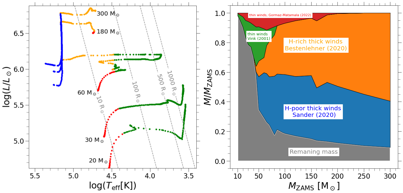
The implementation of $\Gamma_{\rm e}$ as a complementary condition for the initiation of thick winds translates into increased mass loss rates for stars above $60{\rm~{}M}_{\odot}$ at ZAMS. As noticeable in Figure 2, thick winds tend to be initiated comparatively earlier in the evolution of a star the higher its $M_{\rm zams}$ is. The most massive stars almost spend no time at all in their thin winds phase, which leads them to promptly become WNh stars without any prior giant phase. This could potentially explain the lack of red supergiants beyond the Humphrey-Davidson limit (Humphreys & Davidson, 1994) as originally suggested by Mennekens & Vanbeveren (2014).

We report final masses of stars as a function of their initial mass at solar metallicity calculated with MESA and Genec in Figure 3. We have unified the input key physics in both codes in terms of rotation, convection, overshooting, wind mass loss rates. We did not calibrate the codes any further for the results to match. Yet, for the two test models (at $M_{\rm zams}=60{\rm~{}M}_{\odot}$ and $200{\rm~{}M}_{\odot}$) both codes produce almost identical final star masses that show robustness of our predictions. We also show as a comparison the estimates from Martinet et al. (2023) and an approximation of the BH mass distribution from Bavera et al. (2023a). Most of the stars in our models, according to Fryer et al. (2012b), collapse directly into BHs without any SN event. Our estimates show a maximum BH mass from stellar evolution at $Z=0.014$ of $\sim 28{\rm~{}M}_{\odot}$, which comes from stars at $M_{\rm zams}\sim 40{\rm~{}M}_{\odot}$. Below that initial mass, the final star mass increases linearly with $M_{\rm zams}$ and stars do not enter the thick winds regime. Beyond $M_{\rm zams}=40{\rm~{}M}_{\odot}$ stars are subject to thick winds and face increasingly higher mass loss that decreases their final mass. In this context the maximum final mass of a star depends on the onset of thick winds in massive star evolution. All these massive stars subjected to thick winds evolve into compact WR stars.

In contrast with other models like Bavera et al. (2023b) we do not report a quasi-flat distribution of BH masses for the most massive stars in our models. On the contrary, the BH mass slowly increases as a function of ZAMS mass to $M_{\rm BH}=27.7{\rm~{}M}_{\odot}$ for our most massive model with initial mass of $M_{\rm zams}=300{\rm~{}M}_{\odot}$. On the other hand, our models predict lower final star masses than the ones from Martinet et al. (2023) for the highest ZAMS masses. This is due to the fact that in canonical Genec simulations the switch from thin to thick winds is based only on H surface abundance. This makes even the most massive stars to spend significant part of the lifetime in thin (low) wind mass loss regime. In our models very massive stars enter the thick (high) wind mass loss regime very early in the evolution (note that we also use the Eddington factor in addition to surface abundance for the switch). As pointed out in Section 2.1 the upgraded switch using both H surface abundance and the Eddington factor seems in better agreement with observations.

4. Conclusion

Our results do not allow for replication of recent results in context of black hole masses at solar metallicity. We find a different initial–final star mass relation for our updated stellar models. Firstly, our models predict a maximum black hole mass of $\sim 28{\rm~{}M}_{\odot}$ that is smaller by at least $\sim 7{\rm~{}M}_{\odot}$ if compared to Bavera et al. (2023a) and  Martinet et al. (2023). Secondly, our most massive black holes are formed from significantly different initial star masses ($M_{\rm zams}\sim 40{\rm~{}M}_{\odot}$ and $M_{\rm zams}>200{\rm~{}M}_{\odot}$) than the ones found by Bavera et al. (2023a) ($M_{\rm zams}\sim 75{\rm~{}M}_{\odot}$). These differences are understood in terms of the updated wind mass loss prescriptions and the enhanced internal mixing due to rotation and overshooting. Note that we have not only adopted different wind mass loss prescriptions but we have also proposed transition criteria among prescriptions that are more complex than traditionally adopted in modeling of massive stars.

The shape of the initial-final star mass relation at solar metallicity is an important calibration point in the predictions of the overall black hole mass distribution in Universe. LIGO/Virgo/Kagra observatories are sensitive to detecting black holes from a wide range of metallicities (i.e., already reaching galaxies to redshift of $z\sim 1$). Such studies as presented here need to be extended to a full range of metallicities before any reliable conclusions can be made about the black hole mass distribution observed in gravitational-waves. For lower metallicities wind mass loss rates are smaller and final star masses are larger than predicted for $Z=0.014$. This will introduce another key factor/uncertainty in black hole mass calculation: pair-instability pulsations mass loss and stellar disruptions (e.g.,  Farmer et al. (2020)).

We are not claiming that our calculations represent a definitive answer to the question of black hole mass distribution at solar metallicity. Yet, we argue that given the employed recent advancements in massive stellar evolution, this is an incremental step forward in understanding stellar-origin black holes.

5. Appendix: Comparison of old and new wind mass loss prescriptions

The most remarkable difference between old and new wind prescriptions is the value of the mass-loss rate. These lower values of $\dot{M}$ show a better agreement with the actual nature of stellar winds, which are known to be clumped (Bouret et al., 2005; Šurlan et al., 2012, 2013). More detailed theoretical studies on the wind structure of O-type stars, self-consistently coupling radiative acceleration and hydrodynamics in the co-moving frame and non-LTE conditions (Sander et al., 2017; Gormaz-Matamala et al., 2021), have confirmed the same diagnostics.

For thin winds, we observe in Figure 4 that the self-consistent $\dot{M}$ from the m-CAK prescription Gormaz-Matamala et al. (2023) agrees very well with the formula from Krtička & Kubát (2017, 2018) especially for MS stars as outlined by Gormaz-Matamala et al. (2022a). Wind solution from Björklund et al. (2021) also is lower than Vink’s formula, although their $\dot{M}$ is extremely low at low luminosities.

For thick winds, we observe in Figure 4 that both Bestenlehner (2020) and Sander & Vink (2020) provide mass-loss rates below the former Nugis & Lamers (2000). Mass loss for H-rich stars is lower, because it describes the winds of stars in an intermediate evolutionary stage between O-type and WR stars.

However, notice that both panels of Figure 4 only show the relationship $\dot{M}\sim L_{*}$, and straightforwad differences in mass-loss rates at the same luminosity may be misleading. For example lowering mass-loss rates makes stars reach higher luminosities during their evolution (Gormaz-Matamala et al., 2022b, 2023; Björklund et al., 2023), and therefore the mass-loss rates at subsequent evolutionary stages may be larger rather than smaller after adopting updated “lower” wind mass loss prescriptions.

Figure 4.— Comparison of old and new wind prescriptions for thin (left panel) and thick (right panel) winds.

References

- Asplund et al. (2009) Asplund, M., Grevesse, N., Sauval, A. J., & Scott, P. 2009, ARA&A, 47, 481
- Bavera et al. (2023a) Bavera, S. S., et al. 2023a, Nature Astronomy, 7, 1090
- Bavera et al. (2023b) —. 2023b, Nature Astronomy, 7, 1090
- Belczynski et al. (2010a) Belczynski, K., Bulik, T., Fryer, C. L., Ruiter, A., Valsecchi, F., Vink, J. S., & Hurley, J. R. 2010a, ApJ, 714, 1217
- Belczynski et al. (2010b) Belczynski, K., Dominik, M., Bulik, T., O’Shaughnessy, R., Fryer, C. L., & Holz, D. E. 2010b, ApJ, 715, L138
- Belczynski et al. (2022) Belczynski, K., et al. 2022, ApJ, 925, 69
- Bestenlehner (2020) Bestenlehner, J. M. 2020, MNRAS, 493, 3938
- Bestenlehner et al. (2014) Bestenlehner, J. M., et al. 2014, A&A, 570, A38
- Björklund et al. (2021) Björklund, R., Sundqvist, J. O., Puls, J., & Najarro, F. 2021, A&A, 648, A36
- Björklund et al. (2023) Björklund, R., Sundqvist, J. O., Singh, S. M., Puls, J., & Najarro, F. 2023, A&A, 676, A109
- Bouret et al. (2005) Bouret, J. C., Lanz, T., & Hillier, D. J. 2005, A&A, 438, 301
- Brands et al. (2022) Brands, S. A., et al. 2022, A&A, 663, A36
- Castor et al. (1975) Castor, J. I., Abbott, D. C., & Klein, R. I. 1975, ApJ, 195, 157
- Eggenberger et al. (2008) Eggenberger, P., Meynet, G., Maeder, A., Hirschi, R., Charbonnel, C., Talon, S., & Ekström, S. 2008, Ap&SS, 316, 43
- Farmer et al. (2020) Farmer, R., Renzo, M., de Mink, S., Fishbach, M., & Justham, S. 2020, arXiv e-prints, arXiv:2006.06678
- Fryer et al. (2012a) Fryer, C. L., Belczynski, K., Wiktorowicz, G., Dominik, M., Kalogera, V., & Holz, D. E. 2012a, ApJ, 749, 91
- Fryer et al. (2012b) —. 2012b, ApJ, 749, 91
- Georgy et al. (2014) Georgy, C., Saio, H., & Meynet, G. 2014, MNRAS, 439, L6
- Gormaz-Matamala et al. (2023) Gormaz-Matamala, A. C., Cuadra, J., Meynet, G., & Curé, M. 2023, A&A, 673, A109
- Gormaz-Matamala et al. (2019) Gormaz-Matamala, A. C., Curé, M., Cidale, L. S., & Venero, R. O. J. 2019, ApJ, 873, 131
- Gormaz-Matamala et al. (2021) Gormaz-Matamala, A. C., Curé, M., Hillier, D. J., Najarro, F., Kubátová, B., & Kubát, J. 2021, ApJ, 920, 64
- Gormaz-Matamala et al. (2022a) Gormaz-Matamala, A. C., Curé, M., Lobel, A., Panei, J. A., Cuadra, J., Araya, I., Arcos, C., & Figueroa-Tapia, F. 2022a, A&A, 661, A51
- Gormaz-Matamala et al. (2022b) Gormaz-Matamala, A. C., Curé, M., Meynet, G., Cuadra, J., Groh, J. H., & Murphy, L. J. 2022b, A&A, 665, A133
- Gräfener (2021) Gräfener, G. 2021, A&A, 647, A13
- Heger et al. (2000) Heger, A., Langer, N., & Woosley, S. E. 2000, ApJ, 528, 368
- Heger et al. (2005) Heger, A., Woosley, S. E., & Spruit, H. C. 2005, ApJ, 626, 350
- Humphreys & Davidson (1994) Humphreys, R. M., & Davidson, K. 1994, PASP, 106, 1025
- Iglesias & Rogers (1996) Iglesias, C. A., & Rogers, F. J. 1996, ApJ, 464, 943
- Jermyn et al. (2023) Jermyn, A. S., et al. 2023, ApJS, 265, 15
- Köhler et al. (2015) Köhler, K., et al. 2015, A&A, 573, A71
- Krtička & Kubát (2017) Krtička, J., & Kubát, J. 2017, A&A, 606, A31
- Krtička & Kubát (2018) —. 2018, A&A, 612, A20
- Ledoux (1947) Ledoux, P. 1947, ApJ, 105, 305
- Lucy & Solomon (1970) Lucy, L. B., & Solomon, P. M. 1970, ApJ, 159, 879
- Maeder & Meynet (2000) Maeder, A., & Meynet, G. 2000, A&A, 361, 159
- Maeder & Meynet (2004) —. 2004, A&A, 422, 225
- Maeder & Zahn (1998) Maeder, A., & Zahn, J.-P. 1998, A&A, 334, 1000
- Mandel & Broekgaarden (2022) Mandel, I., & Broekgaarden, F. S. 2022, Living Reviews in Relativity, 25, 1
- Martinet et al. (2023) Martinet, S., Meynet, G., Ekström, S., Georgy, C., & Hirschi, R. 2023, arXiv e-prints, arXiv:2309.00062
- Martins & Palacios (2022) Martins, F., & Palacios, A. 2022, A&A, 659, A163
- Mennekens & Vanbeveren (2014) Mennekens, N., & Vanbeveren, D. 2014, A&A, 564, A134
- Nugis & Lamers (2000) Nugis, T., & Lamers, H. J. G. L. M. 2000, A&A, 360, 227
- Paxton et al. (2011) Paxton, B., Bildsten, L., Dotter, A., Herwig, F., Lesaffre, P., & Timmes, F. 2011, ApJS, 192, 3
- Paxton et al. (2013) Paxton, B., et al. 2013, ApJS, 208, 4
- Paxton et al. (2015) —. 2015, ApJS, 220, 15
- Paxton et al. (2018) —. 2018, ApJS, 234, 34
- Paxton et al. (2019) —. 2019, ApJS, 243, 10
- Sabhahit et al. (2023) Sabhahit, G. N., Vink, J. S., Sander, A. A. C., & Higgins, E. R. 2023, MNRAS, 524, 1529
- Sander et al. (2017) Sander, A. A. C., Hamann, W. R., Todt, H., Hainich, R., & Shenar, T. 2017, A&A, 603, A86
- Sander & Vink (2020) Sander, A. A. C., & Vink, J. S. 2020, MNRAS, 499, 873
- Sander et al. (2020) Sander, A. A. C., Vink, J. S., & Hamann, W. R. 2020, MNRAS, 491, 4406
- Scott et al. (2021) Scott, L. J. A., Hirschi, R., Georgy, C., Arnett, W. D., Meakin, C., Kaiser, E. A., Ekström, S., & Yusof, N. 2021, MNRAS, 503, 4208
- Sibony et al. (2023) Sibony, Y., Georgy, C., Ekström, S., & Meynet, G. 2023, arXiv e-prints, arXiv:2310.18139
- Spruit (2002) Spruit, H. C. 2002, A&A, 381, 923
- Tayler (1973) Tayler, R. J. 1973, Monthly Notices of the Royal Astronomical Society, 161, 365
- Tehrani et al. (2019) Tehrani, K. A., Crowther, P. A., Bestenlehner, J. M., Littlefair, S. P., Pollock, A. M. T., Parker, R. J., & Schnurr, O. 2019, MNRAS, 484, 2692
- The LIGO Scientific Collaboration et al. (2023) The LIGO Scientific Collaboration et al. 2023, Physical Review X, 13, 011048
- Vink et al. (2000) Vink, J. S., de Koter, A., & Lamers, H. J. G. L. M. 2000, A&A, 362, 295
- Vink et al. (2001) —. 2001, A&A, 369, 574
- Vink & Gräfener (2012) Vink, J. S., & Gräfener, G. 2012, ApJ, 751, L34
- Vink et al. (2011) Vink, J. S., Muijres, L. E., Anthonisse, B., de Koter, A., Gräfener, G., & Langer, N. 2011, A&A, 531, A132
- Šurlan et al. (2013) Šurlan, B., Hamann, W. R., Aret, A., Kubát, J., Oskinova, L. M., & Torres, A. F. 2013, A&A, 559, A130
- Šurlan et al. (2012) Šurlan, B., Hamann, W. R., Kubát, J., Oskinova, L. M., & Feldmeier, A. 2012, A&A, 541, A37
- Woosley (2017) Woosley, S. E. 2017, ApJ, 836, 244
- Woosley et al. (2002) Woosley, S. E., Heger, A., & Weaver, T. A. 2002, Rev. Mod. Phys., 74, 1015
- Yusof et al. (2013) Yusof, N., et al. 2013, MNRAS, 433, 1114
- Zahn (1992) Zahn, J. P. 1992, A&A, 265, 115