Optimal switching strategies for navigation in stochastic settings

Abstract

Inspired by the intermittent reorientation strategy seen in the behavior of the dung beetle, we consider the problem of the navigation strategy of an active Brownian particle moving in two dimensions. We assume that the heading of the particle can be reoriented to the preferred direction by paying a fixed cost as it tries to maximize its total displacement in a fixed direction. Using optimal control theory, we derive analytically and confirm numerically the strategy that maximizes the particle speed, and show that the average time between reorientations scales inversely with the magnitude of the environmental noise. We then extend our framework to describe execution errors and sensory acquisition noise. Our approach may be amenable to other navigation problems involving multiple sensory modalities that require switching between egocentric and geocentric strategies.

Navigation in noisy environments is fundamental for animal survival in many situations Freas and Cheng (2022); Wiltschko and Wiltschko (2023); Menti et al. (2023). The inherent stochasticity in such tasks emerges from a combination of limited sensory capabilities, complex environments, and execution errors. Given a finite cognitive capacity, animals have to optimally allocate their resources to simultaneously process signals, elaborate a navigation strategy, and execute motion. The extreme examples of how this set of tasks is brought about are commonly known as egocentric and geocentric strategies. A well-known example of the first is seen in the desert ant Cataglyphis Wehner et al. (1996) which relies on continuously updating an internal estimate of the location by integrating sensory and motor information. These egocentric strategies work well by allowing for rapid movement in space but are prone to error accumulation over time due to fluctuating environments and limited memory. At the other extreme is the case of a map-equipped human who relies on geocentric information, using landmarks cues to adjust their strategy. Since this requires probing the environment in real time, a geocentric scheme is slow but more robust to external noise and execution errors. More often than not, one sees a combination of egocentric and geocentric schemes across species Wehner et al. (1996); Peleg and Mahadevan (2016); Haberkern and Jayaraman (2016).

An example of strategy integration is the motion of dung beetles Byrne and Dacke (2011); Baird et al. (2012); Foster et al. (2021); Dacke et al. (2021). In an attempt to escape from the zone of high competition close to a fresh dung pile, dung beetles roll a spheroidal ball of nutrient-rich dung in a fixed direction away from the pile. To persistently move in a straight line, they alternate between rolling and reorientation phases. During the rolling phase, using their dorsal eyes, they acquire directional information from patterns of polarized light and walk backwards, pushing the ball with their hind legs Byrne and Dacke (2011). During the reorientation phases, the beetles climb on top of the ball and dance on it, presumably using long-range cues to correct their heading vid , see Fig. 1. These reorientation events are thought to be triggered by the accumulation of deviations from the preferred direction due to a combination of sensing and execution errors associated with environmental perturbations and dung ball asphericity. Indeed, rougher landscapes lead to more frequent corrections Baird et al. (2012).

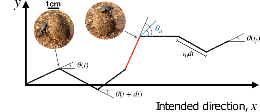
Figure 1: Schematic representation of the navigation model. The agent (e.g. a dung beetle) tries to maximize the displacement in the $x$ direction. It switches between rolling phases, during which it moves at speed $v_{0}$, and reorientation phases (red line), where the direction $\theta$ is reset to the preferred angle $\theta\!=\!0$. The reorientations are triggered when $|\theta|>\theta_{a}(z)$, where $z=x_{c}D/v_{0}$ is a dimensionless measure of noise (see text for details). Images of the dung beetle in the rolling phase and reorientation phases are from ima .

Motivated by this example, here we consider the motion of a sentient agent undergoing correlated random walks Codling et al. (2008) that can switch between egocentric and geocentric strategies to maximize its speed in a given direction, leading to optimal switching protocols determined numerically Peleg and Mahadevan (2016). In this letter, we complement these numerical approaches using optimal control theory Bellman and Kalaba (1965); De Bruyne and Mori (2023), to derive an analytic framework for different strategies in the presence of different sources of noise as well as different models of agent-environment interaction.

We consider an agent moving in a plane with a position $(x(t),y(t))$ with constant speed $v_{0}$, and heading direction $\theta(t)\!\in\![-\pi/2,\pi,2]$. The position and orientation of the agent then evolves according to

$$\dot{x}(t)=v_{0}\cos[\theta(t)]\,,\dot{y}(t)=v_{0}\sin[\theta(t)]\,,\dot{\theta}(t)\!=\!\eta(t)\quad$$ (1)

corresponding to an active Brownian particle Basu et al. (2018), where $\eta(t)$ is zero-mean Gaussian white noise with $\langle\eta(t)\eta(t^{\prime})\rangle\!=\!2D\delta(t-t^{\prime})$ and $D\!>\!0$ is the rotational diffusion . This type of correlated random walk has been widely employed to describe animal navigation towards a target Cheung et al. (2007); Bailey et al. (2018); Yin and Zinn-Björkman (2020); Bijma et al. (2021); Yin and Zinn-Björkman (2022), and assumes that translational Brownian motion is small relative to rotational Brownian motion. Over a characteristic time that scales with $1/D$, the agent will lose its orientational persistence, and in order to maximize its total displacement in the $x$-direction, it must reset its heading to the preferred angle $\theta=0$. We assume that the reorientation process is instantaneous and can be described in terms of an effective displacement lost by stopping for a time $t_{s}$ to correct the direction with a fixed cost $x_{c}\approx v_{0}t_{s}$ for each reorientation.

Assuming an initial condition $x(0)=y(0)=\theta(0)=0$, over a duration $t_{f}$ of the process, we can then define a cost function as the sum of the (negative) distance traveled along the $x-$axis and the distance lost due to $N(t_{f})$ reorientation events in that time as

$$\mathcal{F}=\langle-x(t_{f})+x_{c}N(t_{f})\rangle\,.$$ (2)

A strategy with no reorientation events would lead to the second term vanishing, but the agent would only persist in the initial direction over a distance $\sim v_{0}/D$ Basu et al. (2018); conversely frequent reorientations would result in a large cost, and little progression from the initial state. Thus an optimal strategy is one that minimizes the cost Eq. (2) and depends on the ratio of the resetting cost $x_{c}$ to the persistence length $v_{0}/D$. Defining $z\!\equiv\!x_{c}D/v_{0}$, we expect that for small (large) $z$, the minimization of first (second) term in determines the strategy.

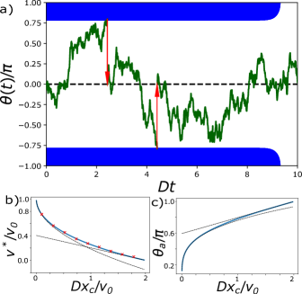
Figure 2: a) Optimal restarting policy for $z\!=\!1$ and $Dt_{f}\!=\!10$, obtained by solving numerically Eq. 3. The optimal strategy is to reset as soon as the angle $\theta(t)$ touches the blue region, while the system evolves freely in the white region (denoted $\Omega(t)$ in the text). The green line shows a typical trajectory with $N\!=\!2$ resetting events (red arrows). b) and c) Optimal speed $v^{*}/v_{0}$ and optimal activation angle $\theta_{a}/\pi$ as a function of $z\!=\!Dx_{c}/v_{0}$. The blue lines correspond to the numerical solution of Eq. 5, while the dashed lines indicate the asymptotic behaviors discussed in the text. The red symbols in b) are the results of Langevin numerical simulations of the optimally controlled dynamics in Eq. (1). The average is performed over a single trajectory with $Dt_{f}=10^{4}$.

Recent studies in non-equilibrium statistical mechanics have shown that resetting a system to its initial position at random times can dramatically improve its search properties Bénichou et al. (2011); Evans and Majumdar (2011a, b); Evans et al. (2020); Kumar et al. (2020); Abdoli and Sharma (2021); Sar et al. (2023). Here, instead of following stochastic resetting protocols, we use an optimal-control framework De Bruyne and Mori (2023) and derive the optimal resetting policy that minimizes the cost in Eq. (2). Defining the optimal cost-to-go $J(\theta,t)$ as the remaining cost of an optimally controlled system starting at $\theta(t)$, i.e. the cost from time $t$ to the final time $t_{f}$, we find that $J(\theta,t)$ satisfies sup

$$-\partial_{t}J(\theta,t)=D\partial^{2}_{\theta}J(\theta,t)-v_{0}\cos(\theta)\,,\quad\theta\in\Omega(t)\,,$$ (3)

where $\Omega(t)=\{\theta:J(\theta,t)\leq J(0,t)+x_{c}\}$. Eq. (3) is a generalization of the Belmann equation Bellman and Kalaba (1965). We note that the nonlinear gradient term of the standard Belmann equation is absent here because the system is controlled through restarts rather than an external force. Eq. (3) must be solved backward in time, with final condition $J(\theta,t_{f})=0$ and Neumann boundary conditions $\partial_{\theta}J(\theta,t)\!=\!0$ for $\theta\!\in\!\partial\Omega(t)$. The domain $\Omega(t)$ determines the optimal resetting policy. By definition, when $\theta\in\Omega(t)$, a reorientation would increase the total cost. Hence, the agent should reorient its direction only if $\theta\notin\Omega(t)$. Since $\Omega(t)$ is dynamically coupled to the solution $J(\theta,t)$, this is a free-boundary problem for (3), well known in the theory of parabolic (diffusion) equations as a Stefan problem Crank (1984) that must in general be solved numerically.

Using an Euler explicit scheme, we integrate numerically Eq. (3), updating the domain $\Omega(t)$ at each timestep. The resulting domain $\Omega(t)$ is shown in Fig. 2a. We find $\Omega(t)=(-\theta_{a},\theta_{a})$, implying that optimal reorientations are triggered when the angle $|\theta|>\theta_{a}(z)$. Close to the final time $t_{f}$, we find $\Omega(t)=[-\pi,\pi]$, meaning that when little time is left, the benefits of a reorientation would no longer outweigh its cost. Indeed, the direction should only be actively controlled for $D(t_{f}-t)\!>\!\log\left(2/(2-z)\right)$ and $z<z_{c}=2$ sup . For $z\geq z_{c}$, the cost is so high that the optimal policy is to let the system evolve freely without reorientations, independently of $t$. On the other hand, when $D(t_{f}-t)\gg 1$ and $z<z_{c}$, the optimal policy becomes time-independent, and the problem can be studied analytically.

In this stationary regime $D(t_{f}-t)\gg 1$, we expect the cost to increase at a constant rate. Plugging the ansatz $J(\theta,t)=j(\theta)+v^{*}t$, which describes the distance traveled after time $t$ into Eq. (3), we find the time-independent equation

$$-v^{*}=D\partial^{2}_{\theta}j(\theta)-v_{0}\cos(\theta)\,,\quad\theta\in[-\theta_{a},\theta_{a}]\,.$$ (4)

Here both $v^{*}$ and the optimal activation angle $\theta_{a}$ are unknown and must be determined by solving Eq. (4) and imposing the boundary conditions $j(\pm\theta_{a})=j(0)+x_{c}$ and $\partial_{\theta}j(\pm\theta)=0$. Doing so, we find that $\theta_{a}$ and $v^{*}$ are given by sup

$$\frac{1}{2}\sin(\theta_{a})\theta_{a}+\cos(\theta_{a})=1-z\,,\\ v^{*}=v_{0}\sin(\theta_{a})/\theta_{a}.$$ (5)

In Figs. 2b and 2c, we show the optimal speed $v^{*}$ and activation angle $\theta_{a}$, in excellent agreement with numerical simulations of Eq. (1) (see sup for details on the simulations). The threshold angle $\theta_{a}(z)$ increases with increasing cost of resetting (or, equivalently, increasing noise); when the cost is small, the optimal threshold is positioned closely to the preferred angle, indicating a more stringent control over the system. In fact, for $z\to 0$, we find the activation angle vanishes as $\theta_{a}\approx(24z)^{1/4}$ and the maximal velocity $v_{0}$ is approached as $v^{*}\approx v_{0}(1-\sqrt{2z/3})$. Furthermore, for $z>z_{c}$, we find $v^{*}=0$.

When $Dt\gg 1$ and $D(t_{f}-t)\gg 1$, the angle $\theta$ reaches a steady state with probability density function (PDF) $P_{\rm ss}(\theta)$. Adopting the first-passage resetting techniques  De Bruyne et al. (2020, 2021), we find

$$P_{\rm ss}(\theta)=\frac{\theta_{a}-|\theta|}{\theta_{a}^{2}}\,,\quad|\theta|<\theta_{a}\,.$$ (6)

Thus, the PDF of $\theta$ is maximal at the preferred direction $\theta=0$ and decays linearly away from it. Similarly, defining $F(T)$ as the PDF of the time $T$ between two orientation events, we find the following scaling form sup ; Redner (2001),

$$F(T) \!=\! \frac{D}{\theta_{a}^{2}}f\left(\frac{DT}{\theta_{a}^{2}}\right),{\rm\leavevmode\nobreak\ \leavevmode\nobreak\ where}$$

$$f(w) \!=\! \pi\sum_{n=0}^{\infty}(-1)^{n}(2n+1)e^{-\pi^{2}(2n+1)^{2}w/4}\,.$$ (7)

This function $f(w)$ is non-monotonic, with a maximum at $w\approx 0.17$ (see Fig. 3), an essential singularity $f(w)\!\approx\!w^{-3/2}e^{-1/(4w)}/\sqrt{\pi}$ as $w\to 0$, and decays exponentially $f(w)\!\approx\!\pi e^{-\pi^{2}w/4}$ for $w\to\infty$. The mean time between correction events is given by $\langle T\rangle=\theta_{a}^{2}/(2D)$ sup . We note that even though the activation angle $\theta_{a}$ increases with increasing noise via Eq. (5), the mean time $\langle T\rangle$ is a decreasing function of $D$, see Fig. 3, in agreement with the empirical observations that reorientations are more frequent in rougher environments Baird et al. (2012). For small $D$, we find $\langle T\rangle\sim 1/\sqrt{D}$, in agreement with Peleg and Mahadevan (2016).

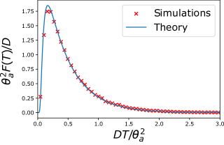
Figure 3: The scaled probability density function $\theta_{a}^{2}F(T)/D$ plotted as a function the scaled time $DT/\theta_{a}^{2}$ between two reorientations. The blue line shows the formula in Eq. (7), while the red crosses are from Langevin numerical simulations of Eq. 1 with $10^{7}$ samples.

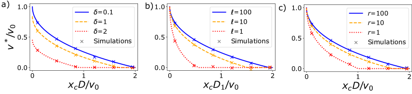
Figure 4: a) Optimal speed $v^{*}/v_{0}$ as a function of the noise parameter $z=x_{c}D/v_{0}$ for different values of a) the magnitude $\delta$ of the execution error, following Eq. 10, b) the ratio $\ell=D_{1}/D_{2}$ of the observable noise to the hidden noise, following Eq. 13, and c) the signal-to-noise ratio $r=D/D_{n}$, following Eq. 14. The crosses are the results of Langevin simulations with $Dt_{f}=10^{4}$.

So far, we have considered the ideal case where the agent has perfect control of its current direction $\theta(t)$. However, motor execution can also be affected by noise Dacke et al. (2021). To incorporate execution errors, we assume that the position of the agent evolves according to

$$\dot{x}(t)=v_{0}\cos[\theta(t)+\epsilon(t)]\,,\dot{y}(t)=v_{0}\sin[\theta(t)+\epsilon(t)]\,,$$ (8)

where the dynamics of $\theta(t)$ is unchanged and the execution error $\epsilon(t)$ is a uniform random variable in $[-\delta,\delta]$, uncorrelated in time. Adapting the optimal control equation (3) to investigate this model sup , we find that the angle $\theta_{a}$ satisfies the modified condition

$$\frac{1}{2}\sin(\theta_{a})\theta_{a}+\cos(\theta_{a})=1-z\frac{\delta}{\sin(\delta)}\,.$$ (9)

We see that the additional noise effectively increases the cost of resetting by a factor $\delta/\sin(\delta)\geq 1$; as $\delta\to 0$, we recover Eq. (5). In this case, the optimal velocity reads sup

$$v^{*}=v_{0}\frac{\sin(\delta)}{\delta}\frac{\sin(\theta_{a})}{\theta_{a}}\,.$$ (10)

Interestingly, even in the limit of low environmental noise $z\to 0$, the optimal speed $v^{*}=v_{0}\sin(\delta)/\delta\leq v_{0}$ is bounded away from the maximal value $v_{0}$ (see Fig. 4a).

In addition to execution noise, experiments show that the angle at which reorientations occur is not constant, i.e. there is uncertainty in sensory acquisition Baird et al. (2012). Indeed, even if the agent has good knowledge of its direction after a reorientation, this knowledge gradually deteriorates over time due to imperfect sensory data, execution errors, and limitations in memory. To account for error accumulation, we first consider the case where the agent has only partial knowledge of its current direction. As an illustrative example, consider the case when the agent’s sensors could only discern the presence of terrain irregularities, while other factors influencing the dynamics of $\theta$ remain unobservable. We consider the dynamics in Eq. (1) but with $\theta(t)$ defined as the sum of two components: $\theta_{1}(t)$, the observable angle, and $\theta_{2}(t)$, the hidden angular deviation. The two angles evolve as $\dot{\theta_{i}}(t)=\eta_{i}(t)$, where $\langle\eta_{i}(t)\eta_{j}(t^{\prime})\rangle=2D_{i}\delta_{ij}\delta(t-t^{\prime})$. We assume that when the agent reorients its direction, both $\theta_{1}(t)$ and $\theta_{2}(t)$ are reset to zero. Hence, the knowledge of $\theta(t)$ is perfect after a reset but degrades over time as $\theta_{2}(t)$ grows.

Since the agent can only make decisions based on the current value of $\theta_{1}$, we consider the control policy of resetting the direction when $|\theta_{1}|\geq\theta_{a}$. For a fixed value of $\theta_{a}$, we compute the steady-state PDF $P_{\rm ss}(\theta)$ of $\theta=\theta_{1}+\theta_{2}$. Calculating $P_{\rm ss}(\theta)$ (see sup for details), we find

$$P_{ss}(\theta)=\frac{1}{\pi\theta_{a}^{2}}\int_{-\infty}^{\infty}dk\leavevmode\nobreak\ e^{-ik\theta}\leavevmode\nobreak\ \frac{1-\frac{\cos(k\theta_{a})}{\cosh\left(k\theta_{a}/\sqrt{\ell}\right)}}{(1+1/\ell)k^{2}}\,,$$ (11)

where $\ell=D_{1}/D_{2}$ is the ratio of the diffusivities of the observable and the hidden angular variables. The velocity in the steady state is then given by

$$v \equiv\lim_{t_{f}\to\infty}\frac{1}{t_{f}}\left[-\int_{0}^{t_{f}}dt\leavevmode\nobreak\ v_{0}\cos(\theta(t))+x_{c}N(t_{f})\right]$$

$$=-v_{0}\langle\cos(\theta)\rangle_{\rm ss}+x_{c}/\langle T\rangle\,,$$ (12)

where $\langle\cdot\rangle_{\rm ss}$ indicates the steady state average in Eq. (11). The average time between reorientations is given by $\langle T\rangle=\theta_{a}^{2}/(2D_{1})$. Using Eq. (11), we find

$$v=\frac{2v_{0}}{\theta_{a}^{2}(1+1/\ell)}\left[1-\frac{\cos(\theta_{a})}{\cosh\left(\theta_{a}/\sqrt{\ell}\right)}\right]-\frac{2v_{0}z}{\theta_{a}^{2}}\,,$$ (13)

where $z=D_{1}x_{c}/v_{0}$. By minimizing this expression as a function of $\theta_{a}$, we find the optimal speed $v^{*}$ sup . Fig. 4b shows that $v^{*}$ increases with $\ell$ for all values of $z$, implying that higher observability leads to higher speed Griffith and Kumar (1971). In the limit $\ell\to\infty$ we recover our original model without measurement errors. Interestingly, at variance with the case of execution errors, the maximal velocity $v_{0}$ can be reached in the low-noise limit $z\to 0$ for all values $\ell$.

As another variant of noisy sensory acquisition we assume that the agent can observe all relevant factors that affect its direction ($\ell\to\infty$), but that these observations are acquired through noisy sensory channels. Thus, although the real direction $\theta$ of the agent evolves as a Brownian motion with diffusion constant $D$, the observed angle is $\theta_{1}(t)=\theta(t)+\theta_{n}(t)$, where $\theta_{n}(t)$ describes the accumulated measurement error. We assume that $\theta_{n}(t)$ independently evolves as a Brownian motion with diffusion constant $D_{n}$ and that after a reorientation both $\theta$ and $\theta_{n}$ are set to zero. The control strategy is again to reorient the direction if $|\theta_{1}|>\theta_{a}$, leading to the speed (see sup for the derivation)

$$v=\frac{2v_{0}}{\theta_{a}^{2}}(1+1/r)\left[1-z-\frac{\cos\left(\frac{\theta_{a}}{1+1/r}\right)}{\cosh\left(\frac{\theta_{a}\sqrt{1/r}}{1+1/r}\right)}\right]\,,$$ (14)

where $z=Dx_{c}/v_{0}$ and $r=D/D_{n}$ is the signal-to-noise ratio. In the limit $r\to\infty$, we recover the results of our original model without sensory noise. In this case, the optimal speed can be obtained by minimizing Eq. (14) with respect to $\theta_{a}\in[0,\pi]$, see Fig. 4c). The qualitative behavior is similar to the previous case. The optimal speed increases with the signal-to-noise ratio and the maximal speed $v_{0}$ is attained for all values of $r$ for $z\to 0$. In sup , we relax the assumption that the reorientation are instantaneous and we show that our framework can be extended to a model with finite-time corrections.

Inspired by the intermittent navigational strategy of the dung beetle, we have identified an optimal strategy that integrates egocentric and geocentric schemes to maximize the speed in a given direction, while accounting for both sensing and actuation errors that lead to a range of testable predictions: the relation between the time between reorientations and noise strength, and the effective speed as a function of errors in measurement and actuation. An immediate question that this raises is that of comparing our results to experimental data on the navigation of dung beetles Foster et al. (2021). More broadly, our approach can also be used in general search situations where the cues about the target location can be obtained from different sensory channels. Indeed this scenario of switching between two modes associated with different modalities of information retrieval and action is quite common, e.g. dogs sniff the ground to get accurate local information and also lift their heads into the boundary layer to get noisy long-range information Thesen et al. (1993), while moths alternate between casting and tracking Reddy et al. (2022); Rigolli et al. (2022). Finally, our model is but a first step in exploring the role of measurement, estimation, representation, sensory integration known to be important in the context of navigation Haberkern and Jayaraman (2016); Kim et al. (2019); future work needs to address this.

This work was supported by a Leverhulme Trust International Professorship Grant (No. LIP-2020-014), the Simons Foundation and the Henri Seydoux Fund.

I Supplemental Material

I.1 Derivation of the optimal control equation

The dynamics of the angle $\theta(t)$ in a small time interval $dt$ can be written as

$$\theta(t+dt)=\begin{cases}\theta(t)+\eta(t)dt\,\quad&\text{if }s(\theta,t)=0\,,\\ 0\quad&\text{if }s(\theta,t)=1\,,\end{cases}$$ (S1)

where $s(\theta,t)$ is a binary variable, describing a reorientation policy. We recall that $\eta(t)$ is Gaussian white noise with zero mean and correlator $\langle\eta(t)\eta(t^{\prime})\rangle=2D\delta(t-t^{\prime})$. Our goal is to identify the optimal policy $s^{*}(\theta,t)$ that minimizes the cost function in Eq. (2) of the main text. We define the cost to-go function

$$\mathcal{F}_{\theta,t}[s]=\left\langle-\int_{t}^{t_{f}}v_{0}\cos(\theta(\tau))dt+x_{c}[N(t_{f})-N(t)]\right\rangle_{\theta}\,,$$ (S2)

which describes the average cost incurred between time $t$ and time $t_{f}$, starting at $\theta$ at time $t$, and following a given policy $s(\theta,t)$. The symbol $\langle\cdot\rangle_{\theta}$ indicates the average with respect to all stochastic trajectories starting at $\theta$ at time $t$. We recall that $v_{0}$ is the speed of the agent and that $N(t)$ indicates the number of reorientations up to time $t$. The cost function $\mathcal{F}_{\theta,t}[s]$ is a functional, depending on the specific form of the function $s=s(\tilde{\theta},\tilde{t})$. The cost function in Eq. (2) of the main text corresponds to $\mathcal{F}=\mathcal{F}_{0,0}[s]$. The optimal cost-to-go $J(\theta,t)$ can be defined as

$$J(\theta,t)=\min_{s}\mathcal{F}_{\theta,t}[s]\,,$$ (S3)

where the minimization is performed over all functions $s(\tilde{\theta},\tilde{t})$, for $\tilde{\theta}\in[-\pi/2,\pi/2]$ and $\tilde{t}\in[t,t_{f}]$.

To perform the minimization, we adopt a dynamic programming approach Bellman and Kalaba (1965). We consider the evolution of the system in a small time interval $dt$, as given in Eq. (S1). Then, Eq. (S2) can be rewritten by splitting the cost incurred in the short time interval $[t,t+dt]$ and in the remaining time interval $[t+dt,t_{f}]$ as

$$\mathcal{F}_{\theta,t}[s]=-v_{0}\cos(\theta)dt+\left(x_{c}+\mathcal{F}_{0,t+dt}[s]\right)s(\theta,t)+\left\langle\mathcal{F}_{\theta+\eta(t)dt,t+dt}[s]\right\rangle(1-s(\theta,t))\,.$$ (S4)

The first term on the right-hand side comes from the integral term in Eq. (S2). In addition, if the system is reset, corresponding to $s(\theta,t)=1$, a unit cost $x_{c}$ is paid and the remaining cost up to time $t_{f}$ is $\mathcal{F}_{0,t+dt}$, since $\theta=0$ after a reorientation. On the other hand, if $s(\theta,t)=0$, the system evolves freely and the new position is $\theta+\eta(t)dt$, leading to the last term in Eq. (S4). Note that $\langle\cdot\rangle$ now indicates averaging over the one-time noise $\eta(t)$, which is a Gaussian random variable with zero mean $\langle\eta(t)\rangle=0$ and variance $\langle\eta(t)^{2}\rangle=2D/dt$.

We perform the minimization in Eq. (S3) in two steps: first we minimize over the binary function $s(\tilde{\theta},\tilde{t})$ for $\tilde{t}\in[t+dt,t_{f}]$ and then over the binary variable $s(\theta,t)$, where $\theta$ and $t$ are fixed. We obtain

$$J(\theta,t)=\min_{s(\theta,t)}\left[-v_{0}\cos(\theta)dt+\left(x_{c}+J(0,t+dt)\right)s(\theta,t)+\left\langle J(\theta+\eta(t)dt,t+dt)\right\rangle(1-s(\theta,t))\right]\,.$$ (S5)

Expanding to first order in $dt$ and using the fact that $s(\theta,t)$ is a bianry variable, we get

$$J(\theta,t)=-v_{0}\cos(\theta)dt+\min\left[x_{c}+J(0,t);J(\theta,t)+\partial_{t}J(\theta,t)dt+D\partial_{\theta}^{2}J(\theta,t)dt\right]\,.$$ (S6)

Therefore, if $x_{c}+J(0,t)\leq J(\theta,t)$ the optimal policy is $s^{*}(\theta,t)=1$ and hence $x_{c}+J(0,t)=J(\theta,t)$. In the opposite case $x_{c}+J(0,t)>J(\theta,t)$, we obtain $s^{*}(\theta,t)=0$ and

$$-\partial_{t}J(\theta,t)=-v_{0}\cos(\theta)+D\partial_{\theta}^{2}J(\theta,t)\,.$$ (S7)

The evolution equation can be rewritten in a more compact form using the domain $\Omega(\theta,t)$ as

$$-\partial_{t}J(\theta,t)=D\partial^{2}_{\theta}J(\theta,t)-v_{0}\cos(\theta)\,,\quad\theta\in\Omega(t)\,,$$ (S8)

where $\Omega(t)=\{\theta:J(\theta,t)<J(0,t)+x_{c}\}$. This differential equation has to be solved with the final condition $J(\theta,t_{f})=0$, which can be obtained by setting $t=t_{f}$ in Eq. (S2). The boundary condition $\partial_{\theta}J(\theta,t)=0$ for $\theta\in\Omega(\theta,t)$ is derived in Ref. De Bruyne and Mori (2023).

We also consider the region where $(t_{f}-t)\ll 1/D$. Indeed, as shown in Fig. 2 in the main text, when the final time $t_{f}$ is approached, the optimal policy is to let the system evolve freely, without reorientations. Hence, in this region, the differential equation is defined over the full interval $[-\pi,\pi]$ (with periodic boundary conditions) and can be solved analytically. The most general solution reads

$$J(\theta,t)=-\frac{v_{0}}{D}(1-e^{-D(t_{f}-t)})\cos(\theta)\,.$$ (S9)

Note that when $D(t-t_{f})\ll 1$, the condition $J(\theta,t)<J(0,t)+x_{c}$ is verified everywhere in $[-\pi,\pi]$. The solution in Eq. (S9) is therefore valid until, increasing $(t_{f}-t)$, the condition $J(\theta,t)=J(0,t)+x_{c}$ is verified for the first time. This occurs at the critical time $t=t^{c}$, where

$$t^{c}=t_{f}-\frac{1}{D}\log\left(\frac{2}{2-z}\right)\,.$$ (S10)

Therefore, if $z<z_{c}=2$, the system is only actively controlled for $t<t^{c}$ and is left free to evolve without reorientations for $t>t^{c}$. For $z\to z_{c}$ the critical time diverges. Hence, for $z>z_{c}$ the cost is too high and it is never convenient to reorient the direction.

I.2 Infinite time horizon solution of the optimal control equation

As explained in the main text, the optimal control policy becomes independent of time in the infinite time-horizon limit, corresponding to $(t_{f}-t)D\gg 1$. In this limit $\Omega=[-\theta_{a},\theta_{a}]$ and the the optimal cost-to-go increases linearly in time. Plugging the ansatz $J(\theta,t)=j(\theta)+v^{*}t$, where $v^{*}$ describes the optimal speed of the agent, into Eq. (S8), we get

$$-v^{*}=Dj^{\prime\prime}(\theta)-v_{0}\cos(\theta)\,,\quad\quad\theta\in\Omega\,,\\$$ (S11)

where

$$\Omega=\{\theta:\,j(\theta)\leq j(0)+x_{c}\}\,.$$ (S12)

The most general solution reads

$$j(\theta)=-\frac{v^{*}}{D}\frac{\theta^{2}}{2}+a\theta+b-\frac{v_{0}}{D}\cos(\theta)\,.$$ (S13)

Assuming that $\Omega=[-\theta_{a},\theta_{a}]$ (to be verified a posteriori), the boundary conditions are

$$j(\pm\theta_{a})=j(0)+x_{c}\,,$$ (S14)

and

$$j^{\prime}(\pm\theta_{a})=0\,.$$ (S15)

From these conditions, we find $a=0$, $v^{*}=v\sin(\theta_{a})/\theta_{a}$, and

$$\frac{1}{2}\sin(\theta_{a})\theta_{a}+\cos(\theta_{a})=1-z\,,$$ (S16)

where $z=Dx_{c}/v_{0}$ is the scaled cost of resetting.

I.3 Steady-state properties

In this section, we investigate the steady-state distribution of the angle $\theta$ in the regime where $tD\gg 1$ and $(t_{f}-t)D\gg 1$. Assuming that the angle $\theta$ is reset to $0$ as soon as $|\theta|>\theta_{a}$, the steady state probability density function $P_{\rm ss}(\theta)$ satisfies the stationary Fokker-Planck equation De Bruyne et al. (2020)

$$0=D\partial^{2}_{\theta}P(\theta)-2\delta(\theta)\left[D\partial_{\theta}P(\theta_{a})\right]\,,$$ (S17)

where the amplitude of the $\delta$ function indicates that the particles flowing at the absorbing barrier at $\theta=\pm\theta_{a}$ are reset at $\theta=0$. The boundary conditions are absorbing, since particles are reset as soon as they reach the bounday at $\theta=\pm\theta_{a}$, corresponding to $P(\pm\theta_{a})=0$. The most general normalized solution that satisfies the boundary conditions reads

$$P_{ss}(\theta)=\frac{\theta_{a}-|\theta|}{\theta_{a}^{2}}\,.$$ (S18)

I.4 Time between two reorientation events

In this section, we compute the distribution of the time $T$ between two subsequent reorientation events. We denote by $S(\theta,t)$ the survival probability, i.e., probability that an angle starting from $\theta$ is not reset up to time $t$.

The survival probability satisfies the backward Fokker-Planck equation Redner (2001)

$$\partial_{t}S=D\partial^{2}_{\theta}S\,,$$ (S19)

with initial condition $S(\theta,0)=1$ and boundary conditions $S(\pm\theta_{a},t)=0$. Taking a Laplace transform with respect to $t$, we find

$$s\tilde{S}(\theta,s)-1=D\partial^{2}_{\theta}\tilde{S}(\theta,s)\,,$$ (S20)

where

$$\tilde{S}(\theta,s)=\int_{0}^{\infty}dt\leavevmode\nobreak\ S(\theta,t)e^{-st}\,.$$ (S21)

Solving the equation and imposing the boundary conditons, we get

$$\tilde{S}(\theta,s)=\frac{1}{s}\left[1-\frac{\cosh\left(\sqrt{\frac{s}{D}}\theta\right)}{\cosh\left(\sqrt{\frac{s}{D}}\theta_{a}\right)}\right]\,.$$ (S22)

We denote by $F(\theta,T)$ the probability density function (PDF) of the time $T$ of the first reorientation event, assuming that the initial angle is $\theta$. Note that, since after a reorientation the angle is set to $\theta=0$, the PDF of the time $T$ between two reorientation events is $F(T)\equiv F(0,T)$.

Using the relation

$$S(\theta,t)=\int_{t}^{\infty}F(\theta,t^{\prime})dt^{\prime}\,,$$ (S23)

we find

$$\tilde{F}(\theta,s)=\int_{0}^{\infty}dt\leavevmode\nobreak\ e^{-st}F(\theta,t)=\frac{\cosh\left(\sqrt{\frac{s}{D}}\theta\right)}{\cosh\left(\sqrt{\frac{s}{D}}\theta_{a}\right)}\,.$$ (S24)

Setting $\theta=0$ we find that the distribution of the time $T$ between resetting events reads

$$F(0,T)=\frac{1}{2\pi i}\int_{\Gamma}ds\leavevmode\nobreak\ e^{sT}\frac{1}{\cosh\left(\sqrt{\frac{s}{D}}\theta_{a}\right)}\,,$$ (S25)

where $\Gamma$ is a Bromwich contour parallel to the imaginary axis in the complex-$s$ plane. Using Cauchy’s residue theorem, we find

$$F(0,T)=\frac{D}{\theta_{a}^{2}}f\left(\frac{DT}{\theta_{a}^{2}}\right)\,,$$ (S26)

where

$$f(w)=\pi\sum_{n=0}^{\infty}(-1)^{n}(2n+1)\exp\left[-\frac{\pi^{2}(2n+1)^{2}w}{4}\right]\,.$$ (S27)

The large-$w$ regime can be immediately obtained from Eq. (S27) by taking the $n=0$ term

$$f(w)\approx\pi e^{-\pi^{2}w/4}\,.$$ (S28)

To investigate the small-$w$ limit, we use Poisson summation formula to find the alternative expression

$$f(w)=\frac{1}{2\sqrt{\pi}}\sum_{m=-\infty}^{\infty}(-1)^{m+1}(2m-1)w^{-3/2}e^{-(2m-1)^{2}/(4w)}\,.$$ (S29)

The small-$w$ behavior is given by the $m=0$ and $m=1$ terms, yielding

$$f(w)\approx\frac{1}{\sqrt{\pi}w^{3/2}}e^{-1/(4w)}\,.$$ (S30)

The mean time $T$ between two resetting events can be evaluated as

$$\langle T\rangle=\int_{0}^{\infty}dt\leavevmode\nobreak\ S(0,t)=\tilde{S}(\theta,0)=\frac{\theta^{2}_{a}}{2D}\,.$$ (S31)

I.5 Execution errors

Here we introduce execution errors in the model. The dynamics of $\theta$ is modified as

$$\begin{cases}\dot{x}(t)=v_{0}\cos(\theta(t)+\epsilon(t))\,,\\ \dot{y}(t)=v_{0}\sin(\theta(t)+\epsilon(t))\,,\\ \dot{\theta}(t)=\eta(t)\,.\end{cases}$$ (S32)

We assume that the measurement noise $\epsilon(t)$ is uniformly distributed in $[-\delta,\delta]$ and uncorrelated in time. Then, the cost function becomes

$$\mathcal{F}=\langle-\int_{0}^{t_{f}}v_{0}\cos(\theta(t)+\epsilon(t))dt+x_{c}n_{r}\rangle\,.$$ (S33)

Performing the average over $\epsilon(t)$, we find

$$\mathcal{F}=\langle-\frac{\sin(\delta)}{\delta}v_{0}\int_{0}^{t_{f}}\cos(\theta(t))dt+x_{c}n_{r}\rangle\,.$$ (S34)

In the limit $\delta\to 0$, we recover the standard case above. For finite $\delta$, the optimal policy will be modified. by rewriting the cost function as

$$\mathcal{F}=\frac{\sin(\delta)}{\delta}\langle-v_{0}\int_{0}^{t_{f}}\cos(\theta(t))dt+\frac{\delta}{\sin(\delta)}x_{c}n_{r}\rangle\,.$$ (S35)

Thus, execution noise increases the effective cost by a factor $\delta/\sin(\delta)\geq 1$, while the overall displacement is scaled by a factor $\sin(\delta)/\delta\leq 1$.

I.6 Partial observations

In this section, we consider the case where the agent has only partial knowledge of its current direction. We assume that the real direction $\theta$ can be affected by various sources of environmental noise. The agent can only detect a subset of these sources. By integrating the available information, the agent derives an estimate, denoted as $\theta_{1}$, of its current direction. The remaining unmeasurable factors give rise to an angle mismatch, denoted as $\theta_{2}$, which grows independently of $\theta_{1}$ over time. We consider the following dynamics

$$\begin{cases}\dot{x}(t)=v\cos(\theta(t))\,,\\ \dot{y}(t)=v\sin(\theta(t))\,,\\ \theta(t)=\theta_{1}(t)+\theta_{2}(t)\,,\\ \dot{\theta}_{1}(t)=\eta_{1}(t)\,,\\ \dot{\theta}_{2}(t)=\eta_{2}(t)\,,,\end{cases}$$ (S36)

where $\eta_{1}$ and $\eta_{2}$ are zero-mean uncorrelated Gaussian white noise with $\langle\eta_{i}(t)\eta_{j}(t^{\prime})\rangle=2D_{i}\delta_{ij}\delta(t-t^{\prime})$. The angle $\theta_{1}$ represents the estimate of the agent of the real direction $\theta$. After a reorientation event, the agent has perfect information on its direction and hence both $\theta_{1}$ and $\theta_{2}$ are set to zero. We consider the average speed

$$v=\lim_{t_{f}\to\infty}\frac{1}{t_{f}}\langle v_{0}\int_{0}^{t_{f}}\cos(\theta(t))dt-x_{c}N(t_{f})\rangle\,,$$ (S37)

where $N(t_{f})$ is the total number of resetting events. We are interested in the restarting policy that minimizes the total cost. Note that in principle this policy could depend on the total time $\tau$ elapsed since the last resetting event, since the amplitude of the noise $\theta_{2}$ grows as $\sqrt{\tau}$. However, here we only focus on time-independent strategies. In other words, we assume that the agent cannot measure $\theta_{2}$ and has to take decisions only knowing $\theta_{1}$. Hence, the optimal strategy consists once again in resetting the system if $|\theta|>\theta_{a}$.

We rewrite the cost average speed as

$$v=v_{0}\langle\cos(\theta)\rangle_{\rm ss}-x_{c}/\langle T\rangle\,,$$ (S38)

where $\langle\cdot\rangle_{\rm ss}$ indicates the steady state average and $T$ is the time between two reorientation. From Eq. (S31), we find $\langle T\rangle=\theta_{a}^{2}/(2D_{1})$. We next compute the steady-state distribution of $\theta=\theta_{1}+\theta_{2}$.

We define $G(\theta,t)$ as the probability density of reaching $\theta$ at time $t$ starting from $\theta_{0}=0$ with no resetting events, i.e., always remaining in the interval $[-\theta_{a},\theta_{a}]$. Similarly, we define $P(\theta,t)$ as the probability density of reaching $\theta$ at time $t$ starting from $\theta_{0}=0$ with any number of resetting events. We also denote by $F(T)$ the distribution of the time $T$ between two successive resetting events. The distribution $P(\theta,t)$ satisfies the relation

$$P(\theta,t)=G(\theta,t)+\int_{0}^{t}dt^{\prime}\leavevmode\nobreak\ F(t^{\prime})P(\theta,t-t^{\prime})\,.$$ (S39)

The first term corresponds to the case where $\theta$ is reached without any resetting events, while the second term describes the case where the first resetting occurs at time $t^{\prime}$. Performing a Laplace transform on both sides, we find

$$\tilde{P}(\theta,s)=\frac{\tilde{G}(\theta,s)}{1-\tilde{F}(s)}\,,$$ (S40)

where we use the notation

$$\tilde{f}(s)=\int_{0}^{\infty}dt\leavevmode\nobreak\ e^{-st}f(t)\,.$$ (S41)

From Eq. (S24), we have

$$\tilde{F}(s)=\frac{1}{\cosh\left(\sqrt{\frac{s}{D_{1}}}\theta_{a}\right)}\,.$$ (S42)

The steady-state distribution

$$P_{ss}(\theta)=\lim_{t\to\infty}P(\theta,t)\,,$$ (S43)

can then be obtained taking the small-$s$ limit

$$P_{ss}(\theta)=\lim_{s\to 0}s\frac{\tilde{G}(\theta,s)}{1-\tilde{F}(s)}\,.$$ (S44)

Using Eq. (S42), we obtain

$$P_{ss}(\theta)=\frac{2D_{1}}{\theta_{a}^{2}}\tilde{G}(\theta,0)=\frac{2D_{1}}{\theta_{a}^{2}}\int_{0}^{\infty}dt\leavevmode\nobreak\ G(\theta,t)\,.$$ (S45)

Therefore, we need to compute the constrained propagator $G(\theta,t)$.

To proceed, we define the propagator $G(\theta_{1},\theta_{2},t)$ as the probability of reaching the angles $\theta_{1}$ and $\theta_{2}$ at time $t$ without resetting, i.e., with the constraint that $|\theta_{1}|<\theta_{a}$ up to time $t$. The propagator satisfies the Fokker-Plank equation

$$\partial_{t}G(\theta_{1},\theta_{2},t)=D_{1}\partial^{2}_{\theta_{1}}G(\theta_{1},\theta_{2},t)+D_{2}\partial^{2}_{\theta_{2}}G(\theta_{1},\theta_{2},t)\,,$$ (S46)

with initial condition $G(\theta_{1},\theta_{2},t=0)=\delta(\theta_{1})\delta(\theta_{2})$ and boundary conditions $G(\theta_{1},\theta_{2},t)=0$ if $|\theta_{1}|=\theta_{a}$. Integrating both sides over $t$ and integrating by parts, we find

$$-\delta(\theta_{1})\delta(\theta_{2})=D_{1}\partial^{2}_{\theta_{1}}\tilde{G}(\theta_{1},\theta_{2},0)+D_{2}\partial^{2}_{\theta_{2}}\tilde{G}(\theta_{1},\theta_{2},0)\,.$$ (S47)

Performing a Fourier transform with respect to $\theta_{2}$, we find

$$-\delta(\theta_{1})=D_{1}\partial^{2}_{\theta_{1}}g(\theta_{1},k)-D_{2}k^{2}g(\theta_{1},k)\,,$$ (S48)

where

$$g(\theta_{1},k)=\int_{-\infty}^{\infty}d\theta_{2}\leavevmode\nobreak\ e^{ik\theta_{2}}\tilde{G}(\theta_{1},\theta_{2},0)\,.$$ (S49)

Solving the differential equation and imposing the boundary conditions, we get

$$g(\theta_{1},k)=\frac{1}{2\sqrt{a}D_{1}}\frac{\sinh(\sqrt{a}(\theta_{a}-|\theta|))}{\cosh(\sqrt{a}\theta_{a})}H(\theta_{a}-|\theta|)\,,$$ (S50)

where $a=D_{2}k^{2}/D_{1}$ and $H(z)$ is the Heaviside step function. Inverting the Fourier transform, we get

$$\tilde{G}(\theta_{1},\theta_{2},0)=\frac{1}{2\pi}\int_{-\infty}^{\infty}dk\leavevmode\nobreak\ e^{-ik\theta_{2}}g(\theta_{1},k)\,.$$ (S51)

Integrating over $\theta_{2}$ keeping $\theta=\theta_{1}+\theta_{2}$ fixed, we find

$$\tilde{G}(\theta,0)=\frac{1}{2\pi}\int_{-\infty}^{\infty}dk\leavevmode\nobreak\ \int_{-\infty}^{\infty}d\theta_{2}\leavevmode\nobreak\ e^{-ik\theta_{2}}g(\theta-\theta_{2},k)\,.$$ (S52)

Evaluating the integral over $\theta_{2}$ with Mathematica, we find

$$\tilde{G}(\theta,0)=\frac{1}{2\pi}\int_{-\infty}^{\infty}dk\leavevmode\nobreak\ e^{-ik\theta}\frac{1}{(D_{1}+D_{2})k^{2}}\left[1-\frac{\cos(k\theta_{a})}{\cosh\left(k\theta_{a}\sqrt{\frac{D_{2}}{D_{1}}}\right)}\right]\,.$$ (S53)

Finally, using Eq. (S45), we obtain the steady state distribution

$$P_{ss}(\theta)=\frac{2D_{1}}{\theta_{a}^{2}}\frac{1}{2\pi}\int_{-\infty}^{\infty}dk\leavevmode\nobreak\ e^{-ik\theta}\frac{1}{(D_{1}+D_{2})k^{2}}\left[1-\frac{\cos(k\theta_{a})}{\cosh\left(k\theta_{a}\sqrt{\frac{D_{2}}{D_{1}}}\right)}\right]\,.$$ (S54)

As a check, we can verify that this distribution is correctly normalized to one

$$\int_{-\infty}^{\infty}d\theta\leavevmode\nobreak\ P_{ss}(\theta)=\frac{2D_{1}}{\theta_{a}^{2}}\int_{-\infty}^{\infty}dk\leavevmode\nobreak\ \delta(k)\frac{1}{(D_{1}+D_{2})k^{2}}\left[1-\frac{\cos(k\theta_{a})}{\cosh\left(k\theta_{a}\sqrt{\frac{D_{2}}{D_{1}}}\right)}\right]=1\,.$$ (S55)

We can now evaluate the average in Eq. (S38)

$$\langle\cos(\theta)\rangle_{\rm ss} =\frac{D_{1}}{\pi\theta_{a}^{2}}\int_{-\infty}^{\infty}d\theta\leavevmode\nobreak\ \cos(\theta)\int_{-\infty}^{\infty}dk\leavevmode\nobreak\ e^{-ik\theta}\frac{1}{(D_{1}+D_{2})k^{2}}\left[1-\frac{\cos(k\theta_{a})}{\cosh\left(k\theta_{a}\sqrt{\frac{D_{2}}{D_{1}}}\right)}\right]$$

$$=\frac{D_{1}}{\theta_{a}^{2}}\int_{-\infty}^{\infty}d\theta\leavevmode\nobreak\ \frac{e^{i\theta}+e^{-i\theta}}{2\pi}\int_{-\infty}^{\infty}dk\leavevmode\nobreak\ e^{-ik\theta}\frac{1}{(D_{1}+D_{2})k^{2}}\left[1-\frac{\cos(k\theta_{a})}{\cosh\left(k\theta_{a}\sqrt{\frac{D_{2}}{D_{1}}}\right)}\right]$$

$$=\frac{D_{1}}{\theta_{a}^{2}}\int_{-\infty}^{\infty}dk\leavevmode\nobreak\ \left[\delta(k+1)+\delta(k-1)\right]\frac{1}{(D_{1}+D_{2})k^{2}}\left[1-\frac{\cos(k\theta_{a})}{\cosh\left(k\theta_{a}\sqrt{\frac{D_{2}}{D_{1}}}\right)}\right]$$

$$=\frac{2D_{1}}{\theta_{a}^{2}}\frac{1}{(D_{1}+D_{2})}\left[1-\frac{\cos(\theta_{a})}{\cosh\left(\theta_{a}\sqrt{\frac{D_{2}}{D_{1}}}\right)}\right]$$ (S56)

Therefore, the speed in Eq. (S38) can be written as

$$v=v_{0}\frac{2D_{1}}{\theta_{a}^{2}}\frac{1}{(D_{1}+D_{2})}\left[1-\frac{\cos(\theta_{a})}{\cosh\left(\theta_{a}\sqrt{\frac{D_{2}}{D_{1}}}\right)}\right]-\frac{2D_{1}x_{c}}{\theta_{a}^{2}}\,,$$ (S57)

which can be rewritten as

$$\frac{v}{v_{0}}=\frac{2}{\theta_{a}^{2}(1+1/\ell)}\left[1-\frac{\cos(\theta_{a})}{\cosh\left(\theta_{a}/\sqrt{\ell}\right)}\right]-\frac{2z}{\theta_{a}^{2}}\,,$$ (S58)

where we have defined $\ell=D_{1}/D_{2}$ and $z=D_{1}x_{c}/v_{0}$. In the limit of low cost $z\to 0$, we find the following asymptotic behaviors

$$\theta_{a}\approx\left(\frac{24\ell}{5+\ell}\right)^{1/4}z^{1/4}\,,$$ (S59)

and

$$\frac{v^{*}}{v_{0}}\approx 1-\sqrt{\frac{2(5+\ell)z}{3\ell}}\,.$$ (S60)

I.7 Measurement errors

In this section, we consider the effect of measurement errors on the navigation strategies. Instead of assuming that the agent has access to only a subset of the factors affecting its direction, we assume that the agent has access to all relevant factors, albeit through noisy sensory channels. As a consequence, the internal representation angle $\theta_{1}$, which the agent employs to approximate the real direction $\theta$, will inevitably deviate from the true $\theta$ over time. To keep things simple, we assume that this deviation, denoted as $\theta_{n}$, grows independently of the actual angle $\theta$. The resulting dynamics read

$$\begin{cases}\dot{x}(t)=v_{0}\cos(\theta(t))\,,\\ \dot{y}(t)=v_{0}\sin(\theta(t))\,,\\ \theta_{1}(t)=\theta(t)+\theta_{n}(t)\,,\\ \dot{\theta}(t)=\eta(t)\,,\\ \dot{\theta}_{n}(t)=\eta_{n}(t)\,,\end{cases}$$ (S61)

where $\eta(t)$ and $\eta_{n}(t)$ are independent Gaussian white noises with zero mean and correlators $\langle\eta(t)\eta(t^{\prime})\rangle=2D\delta(t-t^{\prime})$ and $\langle\eta_{n}(t)\eta_{n}(t^{\prime})\rangle=2D_{n}\delta(t-t^{\prime})$. We denote by $r=D/D_{n}$ the signal-to-noise ratio. Note that, despite the similarity with Eq. (S36), the two models are actually quite different. Note for instance that the variance of the internal angle $\theta_{1}$ is larger than that of the real angle $\theta$ for the model in Eq. (S61), while it is the other way around for Eq. (S36).

Once more, we examine the strategy in which the agent adjusts its direction when $|\theta_{1}|>\theta_{a}$ and we focus on the steady-state properties. As done in the previous section, we first derive the steady-state distribution $P_{\rm ss}(\theta)$ of the real direction $\theta$ for a fixed value of $\theta_{a}$. Eq. (S45) can be easily adapted to the model in Eq. (S61), yielding

$$P_{ss}(\theta)=\frac{2(D+D_{n})}{\theta_{a}^{2}}\int_{0}^{\infty}dt\leavevmode\nobreak\ \int_{-\theta-\theta_{a}}^{-\theta+\theta_{a}}d\theta_{n}\leavevmode\nobreak\ G(\theta,\theta_{n},t)\,,$$ (S62)

where $G(\theta,\theta_{n},t)$ is the probability that $\theta$ and $\theta_{n}$ are reached at time $t$ without any reorientations, assuming that initially $\theta=\theta_{n}=0$.

This probability density satisfies the Fokker-Planck equation

$$\partial_{t}G(\theta,\theta_{n},t)=D\partial^{2}_{\theta}G(\theta,\theta_{n},t)+D_{n}\partial^{2}_{\theta_{n}}G(\theta,\theta_{n},t)\,,$$ (S63)

with boundary conditions $G(\theta,\theta_{n},t)=0$ if $|\theta+\theta_{n}|=\theta_{a}$ and initial condition $G(\theta,\theta_{n},0)=\delta(\theta)\delta(\theta_{n})$. Integrating over $t>0$, we find

$$-\delta(\theta)\delta(\theta_{n})=D\partial^{2}_{\theta}\int_{0}^{\infty}dt\leavevmode\nobreak\ G(\theta,\theta_{n},t)+D_{n}\partial^{2}_{\theta_{n}}\int_{0}^{\infty}dt\leavevmode\nobreak\ G(\theta,\theta_{n},t)\,.$$ (S64)

Making the change of variables $\theta_{1}=\theta+\theta_{n}$ and $w=\theta-w$, we find

$$-2\delta(\theta_{1})\delta(w)=D(\partial_{\theta_{1}}+\partial_{w})^{2}f(\theta_{1},w)+D_{n}(\partial_{\theta_{1}}-\partial_{w})^{2}f(\theta_{1},w)\,,$$ (S65)

where we have defined

$$f(\theta_{1},w)=\int_{0}^{\infty}dt\leavevmode\nobreak\ G\left(\theta=\frac{\theta_{1}+w}{2},\theta_{n}=\frac{\theta_{1}-w}{2},t\right)\,.$$ (S66)

Performing a Fourier transform with respect to $w$, we find

$$-2\delta(\theta_{1})=(D+D_{n})\partial^{2}_{\theta_{1}}\hat{f}(\theta_{1},k)+2ik(D_{n}-D)\partial_{\theta_{1}}\hat{f}(\theta_{1},k)-(D+D_{n})k^{2}\hat{f}(\theta_{1},k)\,,$$ (S67)

where

$$f(\theta_{1},w)=\frac{1}{2\pi}\int_{-\infty}^{\infty}dk\leavevmode\nobreak\ e^{-ikw}\hat{f}(\theta_{1},k)\,.$$ (S68)

Solving the equation and imposing the boundary conditions $\hat{f}(\pm\theta_{a},k)=0$, we find

$$\hat{f}(\theta_{1},k)=\frac{1}{2|k|\sqrt{DD_{n}}}\frac{\exp\left(4|k|(\theta_{a}-|\theta_{1}|)\sqrt{DD_{n}}/(D+D_{n})\right)-1}{\exp\left(4|k|\theta_{a}\sqrt{DD_{n}}/(D+D_{n})\right)+1}\exp\left(i\frac{D-D_{n}}{D+D_{n}}k\theta_{1}+2\frac{\sqrt{DD_{n}}}{D+D_{n}}|k\theta_{1}|\right)\,.$$ (S69)

Combining Eqs. (S62) and (S66), we get

$$P_{ss}(\theta)=\frac{2(D+D_{n})}{\theta_{a}^{2}}\int_{-\theta-\theta_{a}}^{-\theta+\theta_{a}}d\theta_{n}\leavevmode\nobreak\ f(\theta+\theta_{n},\theta-\theta_{n})\,,$$ (S70)

where $f(\theta_{1},w)$ is given in Eq. (S68). We have checked that $P_{ss}(\theta)$ is correctly normalized to one.

Finally, the average velocity can be written as (see Eq. (S38))

$$v=v_{0}\langle\cos(\theta)\rangle_{\rm ss}-x_{c}/\langle T\rangle\,,$$ (S71)

where $\langle\cdot\rangle_{\rm ss}$ denotes the average with respect to $P_{ss}(\theta)$ in Eq. (S70). Performing the average and using $\langle T\rangle=\theta_{a}^{2}/(2(D+D_{n}))$ (see Eq. (S31)), we find

$$\frac{v}{v_{0}}=\frac{2}{\theta_{a}^{2}}(1+1/r)\left[1-\frac{\cos\left(\frac{\theta_{a}}{1+1/r}\right)}{\cosh\left(\frac{\theta_{a}\sqrt{1/r}}{1+1/r}\right)}\right]-\frac{2z}{\theta_{a}^{2}}(1+1/r)\,,$$ (S72)

where $r=D/D_{n}$. In the limit of small cost $z\to 0$, we find

$$\theta_{a}\approx\frac{2^{3/4}3^{1/4}(1+r)^{3/4}}{r^{1/2}(5+r)^{1/4}}z^{1/4}\,,$$ (S73)

and

$$\frac{v^{*}}{v_{0}}\approx 1-\sqrt{\frac{2r^{2}(r+5)z}{3r^{2}(r+1)}}\,.$$ (S74)

I.8 Non-instantaneous reorientations

When a beetle reorients its direction, a finite amount of time is required to operate such correction. So far, we have assumed that the reorientations are instantaneous and we have described this time delay with the effective cost $x_{c}$. Here, we show that our results can be extended to a model where the correction mechanism is explicitly described.

We assume that the animal can switch between two navigation modes: an attention mode and a speed mode. In the first, the agent moves at low speed $v_{1}$ but the direction $\theta(t)$ evolves according to

$$\dot{\theta}(t)=-a\operatorname{sign}(\theta)+\eta(t)\,,$$ (S75)

where $a>0$ is the magnitude of the correcting drift and $\eta(t)$ is as before Gaussian white noise with rotational diffusion constant $D$. The drift continuously steers the angle $\theta$ towards the preferred direction. In the second mode, the agent moves at higher speed $v_{0}>v_{1}$ but has no control over its direction, which evolves as $\dot{\theta}(t)\!=\!\eta(t)$. We do not consider the cost of switching from one mode to the other. The goal is to maximize the displacement $\langle x(t_{f})\rangle$.

The optimal switching strategy can be derived by adapting the Bellman equation (3) to the modified dynamics. However, to investigate the large time-horizon limit ($t_{f}-t\gg D^{-1}$), it is sufficient to study the stationary properties of the dynamics of $\theta$. The optimal strategy is to move with high speed only if $|\theta|<\theta_{a}$, where $\theta_{a}$ has to be chosen to minimize the cost function. Interestingly, the dynamics of $\theta$ can be rewritten as the equilibrium Langevin equation

$$\dot{\theta}(t)=-\partial_{\theta}V(\theta)+\eta(t)\,,$$ (S76)

where the potential $V(\theta)=a(|\theta|-\theta_{a})$ for $|\theta|>\theta_{a}$ and $V(\theta)=0$ otherwise. As a consequence, the stationary state of $\theta$ is given by the equilibrium Boltzmann measure $P_{\rm eq}(\theta)=\exp[-V(\theta)/D]/Z$, where $Z$ is the partition function. By defining $v(\theta)=v_{0}$ if $|\theta|<\theta_{a}$ and $v(\theta)=v_{1}$ otherwise, we can write the average speed as

$$v=\lim_{t_{f}\to\infty}\frac{1}{t_{f}}\int_{0}^{t_{f}}dt\leavevmode\nobreak\ v(\theta(t))\cos(\theta(t))=\langle v(\theta)\cos(\theta)\rangle_{\rm eq}\,,$$ (S77)

where $\langle\cdot\rangle_{\rm eq}$ indicates an average with respect to $P_{\rm eq}(\theta)$. In the case $v_{1}=0$, we find

$$v=v_{0}\frac{\sin(\theta_{a})}{\theta_{a}+\left(1-e^{-{\rm Pe}(\pi-\theta_{a})}\right)/{\rm Pe}}\,,$$ (S78)

where the Péclet number ${\rm Pe}=a/D$ is the ratio of the drift to the diffusion. By minimizing this expression with respect to $\theta_{a}$, we find the optimal speed $v^{*}$ as a function of ${\rm Pe}$, see Figs. S1a and S1b.

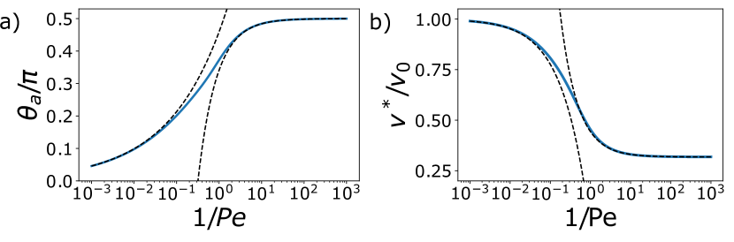
Figure S1: a)Optimal speed $v^{*}/v_{0}$ and activation angle $\theta_{a}/\pi$ as a function of the inverse Péclet number $1/{\rm Pe}=D/a$ in the case of non-instantaneous reorientations with $v_{1}=0$. The dashed lines indicate asymptotic behaviors.

The low-noise behavior (${\rm Pe}\gg 1$) is qualitatively similar to the previous cases. We find that the optimal threshold $\theta_{a}$ approaches zero as $\theta_{a}\approx({\rm Pe}/3)^{-1/3}$ and that the maximal speed $v_{0}$ is approached as $v^{*}\!\approx\!v_{0}-v_{0}({\rm Pe}/3)^{-2/3}/2$. In the high-noise regime ${\rm Pe}\ll 1$, the angle $\theta_{a}$ approaches $\pi/2$ as $\theta_{a}\!\approx\!\pi/2-2{\rm Pe}$. Indeed, when $|\theta|>\pi/2$, the agent is moving in the wrong direction and it is therefore convenient to switch to the slow state, regardless of the noise level. The resulting speed behaves as $v^{*}\!\approx\!v_{0}(1/\pi+{\rm Pe}/8)$. The asymptotic value $v_{0}/\pi$ can be explained by the fact that, in the high-noise limit, the equilibrium PDF of $\theta$ approaches a uniform distribution over $[-\pi,\pi]$.

II Numerical simulations

In this section, we describe the details of the numerical simulations presented in the main text. To verify our analytical predictions we implement a standard Langevin algorithm. In the stationary regime $D(t_{f}-t)\gg 1$ the optimal strategy is time-independent. Hence, in a small time interval $dt$ the optimal dynamics of the direction $\theta$ reads

$$\theta(t+dt)=\begin{cases}\theta(t)+\sqrt{2Ddt}\eta(t)\,\quad&\text{ if }|\theta(t)|<\theta_{a}\,,\\ 0\,\quad&\text{ if }|\theta(t)|>\theta_{a}\,,\end{cases}$$ (S79)

where $\eta(t)$ is a zero-mean unit-variance Gaussian variable and $\theta_{a}$ is the solution of the transcendental equation (5) for a given noise level $z=Dx_{c}/v_{0}$. For each value of $z$, we generate numerically a single trajectory of duration $t_{f}=10^{4}$. We choose $v_{0}=1$, $x_{c}=z$, $D=1$ and $dt=0.01$. Finally, the average speed is evaluated as the time average

$$v^{*}\approx\frac{1}{t_{f}}\left[\int_{0}^{t_{f}}v_{0}\cos(\theta(t))dt-x_{c}N(t_{f})\right]\,,$$ (S80)

where $N(t)$ is the total number of reorientation events up to time. This algorithm can be easily adapted to the models of sensory or motor noise.

To evaluate the average time $T$ between two reorientation events, we integrate Eq. (S79) starting from $\theta(t=0)=0$ and stopping the dynamics when a reorientation occurs for the first time. We repeat this procedure to obtain $10^{7}$ samples.

References

Freas and Cheng (2022)C. A. Freas and K. Cheng, Annu. Rev.
Psychol. 73, 217
(2022).
Wiltschko and Wiltschko (2023)R. Wiltschko and W. Wiltschko, Eur
Phys J Spec Top 232, 237
(2023).
Menti et al. (2023)G. M. Menti, N. Meda,
M. A. Zordan, and A. Megighian, Eur. J. Neurosci. 57, 1980 (2023).
Wehner et al. (1996)R. Wehner, B. Michel, and P. Antonsen, J. Exp. Biol. 199, 129 (1996).
Peleg and Mahadevan (2016)O. Peleg and L. Mahadevan, Royal Soc. Open Sci. 3, 160128 (2016).
Haberkern and Jayaraman (2016)H. Haberkern and V. Jayaraman, Curr. Opin. Neurobiol. 37, 59 (2016).
Byrne and Dacke (2011)M. Byrne and M. Dacke, The visual ecology of dung beetles,
in L. W. Simmons & T. J. Ridsill-Smith (Eds.), Ecology and evolution of dung
beetles (John Wiley & Sons, Chichester, U.K., 2011) pp. 177–199.
Baird et al. (2012)E. Baird, M. J. Byrne,
J. Smolka, E. J. Warrant, and M. Dacke, PLoS One 7, e30211 (2012).
Foster et al. (2021)J. J. Foster, C. Tocco,
J. Smolka, L. Khaldy, E. Baird, M. J. Byrne, D.-E. Nilsson, and M. Dacke, Curr. Biol. 31, 3935 (2021).
Dacke et al. (2021)M. Dacke, E. Baird,
B. El Jundi, E. J. Warrant, and M. Byrne, Annu. Rev. Entomol. 66, 243 (2021).
Codling et al. (2008)E. A. Codling, M. J. Plank,
and S. Benhamou, J R Soc
Interface 5, 813
(2008).
Bellman and Kalaba (1965)R. Bellman and Kalaba, Dynamic programming and modern control theory, Vol. 81 (Academic Press, New
York, 1965).
De Bruyne and Mori (2023)B. De Bruyne and F. Mori, Phys.
Rev. Research 5, 013122
(2023).
Basu et al. (2018)U. Basu, S. N. Majumdar,
A. Rosso, and G. Schehr, Phys. Rev. E 98, 062121 (2018).
Note (1)A more appropriate description of the noise would be via a
von-Mises distribution that correctly accounts for the periodicity of , but for low noise levels, as assumed here, we can neglect the difference
between the two.
Cheung et al. (2007)A. Cheung, S. Zhang,
C. Stricker, and M. V. Srinivasan, Biol. Cybern. 97, 47 (2007).
Bailey et al. (2018)J. D. Bailey, J. Wallis, and E. A. Codling, Ecology 99, 217 (2018).
Yin and Zinn-Björkman (2020)Z. Yin and L. Zinn-Björkman, J. Theor. Biol. 486, 110106 (2020).
Bijma et al. (2021)N. N. Bijma, A. E. Filippov,
and S. N. Gorb, J. Theor. Biol. 520, 110659 (2021).
Yin and Zinn-Björkman (2022)Z. Yin and L. Zinn-Björkman, Theor. Ecol. 15, 17 (2022).
Bénichou et al. (2011)O. Bénichou, C. Loverdo, M. Moreau, and R. Voituriez, Rev. Mod. Phys. 83, 81 (2011).
Evans and Majumdar (2011a)M. R. Evans and S. N. Majumdar, Phys. Rev. Lett. 106, 160601 (2011a).
Evans and Majumdar (2011b)M. R. Evans and S. N. Majumdar, J.
Phys. A Math. Theor. 44, 435001 (2011b).
Evans et al. (2020)M. R. Evans, S. N. Majumdar,
and G. Schehr, J. Phys. A Math.
Theor. 53, 193001
(2020).
Kumar et al. (2020)V. Kumar, O. Sadekar, and U. Basu, Phys. Rev. E 102, 052129 (2020).
Abdoli and Sharma (2021)I. Abdoli and A. Sharma, Soft
Matter 17, 1307
(2021).
Sar et al. (2023)G. K. Sar, A. Ray, D. Ghosh, C. Hens, and A. Pal, Soft Matter 19, 4502 (2023).
(30)See Supplemental Material.
Crank (1984)J. Crank, Free and moving boundary
problems (Oxford University Press, New York, 1984).
De Bruyne et al. (2020)B. De Bruyne, J. Randon-Furling, and S. Redner, Phys.
Rev. Lett. 125, 050602
(2020).
De Bruyne et al. (2021)B. De Bruyne, J. Randon-Furling, and S. Redner, J.
Stat. Mech. Theory Exp. 2021, 013203 (2021).
Redner (2001)S. Redner, A guide to first-passage
processes (Cambridge university press, 2001).
Griffith and Kumar (1971)E. W. Griffith and K. Kumar, J.
Math. Anal. Appl. 35, 135 (1971).
Thesen et al. (1993)A. Thesen, J. B. Steen, and K. B. Døving, J. Exp. Biol. 180, 247 (1993).
Reddy et al. (2022)G. Reddy, V. N. Murthy, and M. Vergassola, Annu. Rev.
Condens. Matter Phys. 13, 191 (2022).
Rigolli et al. (2022)N. Rigolli, G. Reddy,
A. Seminara, and M. Vergassola, Elife 11 (2022).
Kim et al. (2019)S. S. Kim, A. M. Hermundstad, S. Romani,
L. Abbott, and V. Jayaraman, Nature 576, 126 (2019).