Double-Virtual NNLO QCD Corrections for Five-Parton Scattering:
The Quark Channels

Abstract

We complete the computation of two-loop helicity amplitudes required to obtain next-to-next-to-leading order QCD corrections for three-jet production at hadron colliders, including all contributions beyond the leading-color approximation. The analytic expressions are reconstructed from finite-field samples obtained with the numerical unitarity method. We find that the reconstruction is significantly facilitated by exploiting the overlaps between rational coefficient functions of quark and gluon processes, and we display their compact generating sets in the appendix of the paper. We implement our results in a public code, and demonstrate its suitability for phenomenological applications.

I Introduction

Scattering processes that produce multiple jets in the final states are abundant at the Large Hadron Collider. In the next decades, precise theory predictions suitable for analyzing the expected large event samples will be crucial for advancing our understanding of high-energy interactions. Historically, pure-QCD predictions aimed at multi-jet production have also played an important role in the discovery of new structures and methods in field-theory, which inspire neighboring fields.

The goal of this work are predictions for the five-parton processes in QCD, which have been an active field of research for many years. Tree-level five-point amplitudes in QCD were derived a long time ago in 1985 Parke:1985pn. About a decade later the one-loop amplitudes were obtained Bern:1993mq; Kunszt:1994nq; Bern:1994fz. The increase in analytic and algebraic complexity of two-loop computations required significant theoretical and technical developments over the following 20 years. This led to the five-point two-loop amplitudes for the all-plus helicity configuration to be first computed numerically Badger:2013gxa and later in analytic form Gehrmann:2015bfy; Dunbar:2016aux. By now, the five-parton two-loop amplitudes with all helicity configurations are known in the leading-color approximation Badger:2017jhb; Abreu:2017hqn; Badger:2018gip; Abreu:2018jgq; Badger:2018enw; Abreu:2018zmy; Abreu:2019odu; Abreu:2021oya.

These results opened the door for the first computation of next-to-next-to-leading order (NNLO) QCD predictions for three-jet production Czakon:2021mjy (see also Chen:2022ktf), and the follow-up measurements of the strong coupling constant at high scales Czakon:2021mjy; ATLAS:2023tgo; Alvarez:2023fhi. The double-virtual corrections Abreu:2021oya, contributing on average about $10\%$ Czakon:2021mjy, have been included in the leading color approximation in these works. This highlights the potential importance of including subleading-color effects.

In the preceding publication DeLaurentis:2023nss we have obtained the analytic expressions for the five-point gluon amplitudes including all color contributions. Computing the mixed quark and gluon channels is the central goal of this work, which completes the two-loop five-parton scattering amplitudes.

The computation of the non-planar five-point amplitudes is a multi-layered challenge, due to its analytic and combinatorial complexity. We rely on a number of recent results and methods. We use the massless five-point Feynman integrals Papadopoulos:2015jft; Gehrmann:2018yef; Abreu:2018aqd; Chicherin:2018old; Chicherin:2020oor, rely on the geometric methods for obtaining integration-by-parts identities Gluza:2010ws; vonManteuffel:2014ixa; Ita:2015tya; Larsen:2015ped; Bern:2017gdk, and we employ analytic reconstruction methods Peraro:2016wsq; Klappert:2020nbg; Magerya:2022hvj; Belitsky:2023qho; DeLaurentis:2022otd; Badger:2021imn; Abreu:2021asb; Liu:2023cgs; DeLaurentis:2019bjh; DeLaurentis:2020qle; Campbell:2022qpq. In our computation we closely follow our recent work DeLaurentis:2023nss. We apply the numerical unitarity method Ita:2015tya; Abreu:2017xsl; Abreu:2017hqn; Abreu:2020xvt; Abreu:2023bdp to compute numerical values for the scattering amplitudes, which we use to reconstruct analytic results. The computation relies on the spinor-helicity formalism, which in turn yields very compact expressions as displayed in the appendices. In order to reduce the computational load, we develop an efficient way to obtain a large portion of quark amplitudes from gluon amplitudes. In fact, we rescale gluon amplitudes in a way reminiscent of supersymmetry Ward identities Grisaru:1977px; Grisaru:1976vm; Parke:1985pn. The remaining parts of the amplitude are obtained applying a variant of a recent analytic reconstruction technique Abreu:2023bdp.

The analytic results for amplitudes are provided in ancillary files, suitable for future theoretical and phenomenological studies. In particular, we provide a C++ library for fast and stable numerical evaluation of our analytic results. Together with the gluon channel, presented in the first part of this work DeLaurentis:2023nss, these results will provide crucial input for NNLO predictions for three-jet and for N³LO di-jet production in hadron collisions.

Note added: while this work was in preparation, partially overlapping results were reported Agarwal:2023suw. We thank the authors of ref. Agarwal:2023suw for correspondence on numerical comparison between our results.

II Notation and Conventions

II.1 Helicity amplitudes

We consider the channels of the five-parton scattering in QCD that involve external quarks. We associate indices 1 and 2 to the initial state partons and 3, 4 and 5 to final states. There are three channels with a pair of quark and anti-quark,

$$\bar{u}_{-p_{1}}^{-h_{1}}+u_{-p_{2}}^{-h_{2}}\to g_{p_{3}}^{h_{3}} +g_{p_{4}}^{h_{4}}+g_{p_{5}}^{h_{5}}\,,$$ (1)

$$\bar{u}_{-p_{1}}^{-h_{1}}+g_{-p_{2}}^{-h_{2}}\to\bar{u}_{p_{3}}^{h_{3}} +g_{p_{4}}^{h_{4}}+g_{p_{5}}^{h_{5}}\,,$$ (2)

$$g_{-p_{1}}^{-h_{1}}+g_{-p_{2}}^{-h_{2}}\to u_{p_{3}}^{h_{3}} +{\bar{u}}_{p_{4}}^{h_{4}}+g_{p_{5}}^{h_{5}}\,.$$ (3)

Without loss of generality we denote the quarks with $u$ for up-type quark. There are four quark channels with distinct quark flavors, chosen to be up-type and down-type quarks,

$$\bar{u}_{-p_{1}}^{-h_{1}}+u_{-p_{2}}^{-h_{2}}\to d_{p_{3}}^{h_{3}} +\bar{d}_{p_{4}}^{h_{4}}+g_{p_{5}}^{h_{5}}\,,$$ (4)

$$\bar{u}_{-p_{1}}^{-h_{1}}+d_{-p_{2}}^{-h_{2}}\to d_{p_{3}}^{h_{3}} +\bar{u}_{p_{4}}^{h_{4}}+g_{p_{5}}^{h_{5}}\,,$$ (5)

$$\bar{u}_{-p_{1}}^{-h_{1}}+\bar{d}_{-p_{2}}^{-h_{2}}\to\bar{d}_{p_{3}}^{h_{3}} +\bar{u}_{p_{4}}^{h_{4}}+g_{p_{5}}^{h_{5}}\,,$$ (6)

$$\bar{u}_{-p_{1}}^{-h_{1}}+g_{-p_{2}}^{-h_{2}}\to\bar{u}_{p_{3}}^{h_{3}} +d_{p_{4}}^{h_{4}}+\bar{d}_{p_{5}}^{h_{5}}\,.$$ (7)

All other channels involving distinct quark flavors are related to the above by charge conjugation and permutation of labels. The three channels with four identical quark flavors are obtained as linear combination of the distinct quark ones,

$$\bar{u}_{-p_{1}}^{-h_{1}}+ u_{-p_{2}}^{-h_{2}}\to u_{p_{3}}^{h_{3}}+\bar{u}_{p_{4}}^{h_{4}}+g_{p_{5}}^{h_{5}}=$$ (8)

$$\big{(}\bar{u}_{-p_{1}}^{-h_{1}}+u_{-p_{2}}^{-h_{2}}\to d_{p_{3}}^{h_{3}}+\bar{d}_{p_{4}}^{h_{4}}+g_{p_{5}}^{h_{5}}\big{)}-$$

$$\big{(}\bar{u}_{-p_{1}}^{-h_{1}}+d_{-p_{2}}^{-h_{2}}\to d_{p_{3}}^{h_{3}}+\bar{u}_{p_{4}}^{h_{4}}+g_{p_{5}}^{h_{5}}\big{)}\,,$$

$$\bar{u}_{-p_{1}}^{-h_{1}}+ \bar{u}_{-p_{2}}^{-h_{2}}\to\bar{u}_{p_{3}}^{h_{3}}+\bar{u}_{p_{4}}^{h_{4}}+g_{p_{5}}^{h_{5}}=$$ (9)

$$\big{(}\bar{u}_{-p_{1}}^{-h_{1}}+\bar{u}_{-p_{2}}^{-h_{2}}\to\bar{d}_{p_{3}}^{h_{3}}+\bar{d}_{p_{4}}^{h_{4}}+g_{p_{5}}^{h_{5}}\big{)}-$$

$$\big{(}\bar{u}_{-p_{1}}^{-h_{1}}+\bar{d}_{-p_{2}}^{-h_{2}}\to\bar{d}_{p_{3}}^{h_{3}}+\bar{u}_{p_{4}}^{h_{4}}+g_{p_{5}}^{h_{5}}\big{)}\,,$$

$$\bar{u}_{-p_{1}}^{-h_{1}}+ g_{-p_{2}}^{-h_{2}}\to\bar{u}_{p_{3}}^{h_{3}}+u_{p_{4}}^{h_{4}}+\bar{u}_{p_{5}}^{h_{5}}=$$ (10)

$$\big{(}\bar{u}_{-p_{1}}^{-h_{1}}+g_{-p_{2}}^{-h_{2}}\to\bar{u}_{p_{3}}^{h_{3}}+d_{p_{4}}^{h_{4}}+\bar{d}_{p_{5}}^{h_{5}}\big{)}-$$

$$\big{(}\bar{u}_{-p_{1}}^{-h_{1}}+g_{-p_{2}}^{-h_{2}}\to\bar{d}_{p_{3}}^{h_{3}}+d_{p_{4}}^{h_{4}}+\bar{u}_{p_{5}}^{h_{5}}\big{)}\,.$$

Representative diagrams for the two-loop contributions are collected in table 1 and 2.

Throughout this article we use two interchangeable notations to specify the particles’ helicities. We either give signs $\pm$ to label positive/negative helicities or, equivalently, the (half-)integers $h=\pm 1/2$ and $h=\pm 1$ to provide a better distinction between the quark and gluon helicities, respectively.

Whenever we use the arrow notation ($\to$), the first two particles are to be understood as crossed to be incoming, such that their quantum numbers and momenta are given in incoming convention, while the final states are understood in out-going convention. If no arrow ($\to$) is used we consider the all-outgoing convention.

Table 1: Representative Feynman diagrams for two-quark three-gluon amplitudes, contributing at order $N^{0}_{f}$, $N^{1}_{f}$ and $N^{2}_{f}$.

Table 2: Representative Feynman diagrams for four-quark one-gluon amplitudes, contributing at order $N^{0}_{f}$, $N^{1}_{f}$ and $N^{2}_{f}$.

II.2 Kinematics and permutation groups

We consider the scattering of five massless particles using the same conventions as in ref. DeLaurentis:2023nss. The kinematic is defined with five Mandelstam invariants $\{s_{12},s_{23},s_{34},s_{45},s_{15}\}$, together with the parity-odd contraction ${\rm tr}_{5}=\tr(\gamma^{5}\not{p}_{1}\not{p}_{2}\not{p}_{3}\not{p}_{4})$.

The particles’ helicity states are specified using two-component spinors, $\lambda_{i}^{\alpha}$ and $\tilde{\lambda}_{i}^{\dot{\alpha}}$, with $i\in\{1,\dots,5\}$. We define spinor brackets as the contractions,

$$\langle ij\rangle=\lambda^{\alpha}_{i}\lambda_{j,\alpha}\quad\text{and}\quad[ij]=\tilde{\lambda}_{i,\dot{\alpha}}\tilde{\lambda}_{j}^{\dot{\alpha}}\,,$$ (11)

which are linked to Mandelstam invariants through $s_{ij}=\langle ij\rangle[ji]$ (see e.g. Maitre:2007jq for matching conventions). We will also use a shorthand for spinor chains,

$$\langle i|j\pm k|i]=\langle ij\rangle[ji]\pm\langle ik\rangle[ki]\,,$$ (12)

and we write ${\rm tr}_{5}$ as

$${\rm tr}_{5}=[12]\langle 23\rangle[34]\langle 41\rangle-\langle 12\rangle[23]\langle 34\rangle[41]\,.$$ (13)

Under Lorentz transformations, spinor contractions have a residual covariance under little-group transformations. In fact, a little-group transformation of the $i^{th}$ leg with helicity $h_{i}$ reads $(\lambda_{i},\tilde{\lambda}_{i})\rightarrow(z_{i}\lambda_{i},\tilde{\lambda}_{i}/z_{i})$. Accordingly, helicity amplitudes transform as $A\rightarrow z_{i}^{-2h_{i}}A$. We refer to the exponent of the $z_{i}$ as the little-group weight. In summary, helicity amplitudes are homogeneous expressions of spinor brackets not just w.r.t. the total degree but also w.r.t each little-group weight.

Finally, throughout the article we will denote the group of cyclic permutations of $n$ elements $\{i_{1},\ldots{},i_{n}\}$ by ${{\cal Z}_{n}}(i_{1},\ldots{},i_{n})$ and the set of all permutations of $n$ elements, the symmetric permutation group, by ${\cal S}_{n}(i_{1},\ldots{},i_{n})$.

II.3 Color space

The external gluons are in the adjoint representation of $SU(N_{c})$, with indices denoted as $a,b,c$ or $a_{k}$, which run over over $N_{c}^{2}-1$ values. Quarks carry (anti-)fundamental color indices $i,j$ ($\bar{i},\bar{j}$) or $i_{k}$ ($\bar{i}_{k}$), which assume $N_{c}$ values. Both color indices will be collected in tuples $\vec{a}=\{a_{1},\ldots{},a_{n},i_{1},\bar{i}_{1},\ldots{},\bar{i}_{n}\}$. We explicitly represent the parton amplitudes in the color space through the trace basis as in ref. Bern:1990ux.

We use the shorthand notation $\tr(i_{1},\ldots{},i_{n})=\tr(T^{a_{i_{1}}}\cdots{}T^{a_{i_{n}}})$, and $(T^{a})^{\,\bar{i}}_{i}$ are the hermitian and traceless generators of the fundamental representation of $SU(N_{c})$.

The generators $T^{a}$ are normalized as,

$${\tr}(T^{a}T^{b})=\delta^{ab}\,,$$ (14)

and fulfill the commutator relations,

$$\left[T^{a},T^{b}\right] =if_{abc}T^{c}\,,$$ (15)

$$if_{abc} =\tr(T^{a}T^{b}T^{c})-\tr(T^{b}T^{a}T^{c})\,.$$ (16)

The color algebra used in this paper is obtained from applying the Fierz identity,

$$(T^{a})^{\,\,\bar{i}}_{i}(T^{a})^{\,\,\bar{j}}_{j}=\delta^{\bar{i}}_{j}\delta^{\bar{j}}_{i}-\frac{1}{N_{c}}\delta^{\bar{i}}_{i}\delta^{\bar{j}}_{j}\,.$$ (17)

which allows to evaluate the summation over adjoint indices.

Using the above notation, the three-gluon two-quark scattering amplitudes are decomposed in color structures as

$$\mathcal{A}_{\vec{a}}(1_{u},2_{\bar{u}},3_{g},4_{g},5_{g})=\\ \sum_{\sigma\in\mathcal{S}_{3}(3,4,5)}\sigma\Big{(}(T^{a_{3}}T^{a_{4}}T^{a_{5}})^{\,\bar{i}_{2}}_{i_{1}}\;A_{1}(1,2,3,4,5)\Big{)}\;+\\ \sum_{\sigma\in\frac{\mathcal{S}_{3}(3,4,5)}{\mathcal{Z}_{2}(3,4)}}\sigma\Big{(}\tr(3,4)(T^{a_{5}})^{\,\bar{i}_{2}}_{i_{1}}\;A_{2}(1,2,3,4,5)\Big{)}\;+\\ \sum_{\sigma\in\frac{\mathcal{S}_{3}(3,4,5)}{\mathcal{Z}_{3}(3,4,5)}}\sigma\Big{(}\tr(3,4,5)\delta^{\bar{i}_{2}}_{i_{1}}A_{3}(1,2,3,4,5)\Big{)}\;.$$ (18)

Here $\sigma=\{\sigma_{1},\ldots{},\sigma_{5}\}$ denotes permutations which acts on all external-particle labels as $\sigma(i)=\sigma_{i}$. The sums run over all permutations that do not leave the respective color structures invariant, i.e. over 6, 3, and 2 elements in the three lines of eq. 18, respectively.

Similarly, the one-gluon four-quark amplitudes are given by,

$$\mathcal{A}_{\vec{a}}(1_{u},2_{\bar{u}},3_{d},4_{\bar{d}},5_{g})=\\ \sum_{\sigma\in\mathcal{Z}_{2}(\{1,2\},\{3,4\})}\sigma\Big{(}\delta^{\bar{i}_{4}}_{i_{1}}(T^{a_{5}})^{\,\bar{i}_{2}}_{i_{3}}\;A_{4}(1,2,3,4,5)\Big{)}\;+\\ \kern-28.45274pt\sum_{\sigma\in\mathcal{Z}_{2}(\{1,2\},\{3,4\})}\kern-5.69054pt\sigma\Big{(}\delta^{\bar{i}_{2}}_{i_{1}}(T^{a_{5}})^{\,\bar{i}_{4}}_{i_{3}}\;A_{5}(1,2,3,4,5)\Big{)}\,,\kern-2.84526pt$$ (19)

where the sums run over exchanging quarks pairs.

The amplitudes $A_{i}$ admit an expansion in terms of the bare QCD coupling constant $\alpha_{s}^{0}=(g_{s}^{0})^{2}/(4\pi)$,

$$A_{i}=(g_{s}^{0})^{3}\left(\sum_{L=0}^{2}\left(\frac{\alpha_{s}^{0}}{2\pi}\right)^{L}A_{i}^{(L)}\leavevmode\nobreak\ +\leavevmode\nobreak\ \order{(\alpha_{s}^{0})^{3}}\right)$$ (20)

with $L$ denoting the number of loops.

The amplitudes can be further expanded in powers of $N_{c}$ and $N_{f}$ through two loops. For the two-quark amplitudes we obtain the following decomposition,

$$A_{1}^{(0)} =A_{1}^{(0),(0,0)}\,,\quad A_{2}^{(0)}=0\,,\quad A_{3}^{(0)}=0\,,$$ (21a)

$$A_{1}^{(1)} =N_{c}\leavevmode\nobreak\ A_{1}^{(1),(1,0)}+\frac{1}{N_{c}}A_{1}^{(1),(-1,0)}+N_{f}A_{1}^{(1),(0,1)}\,,\quad A_{2}^{(1)}=A_{2}^{(1),(0,0)}+\frac{N_{f}}{N_{c}}A_{2}^{(1),(-1,1)}\,,$$ (21b)

$$A_{3}^{(1)} =A_{3}^{(1),(0,0)}+\frac{N_{f}}{N_{c}}A_{3}^{(1),(-1,1)}\,,$$ (21c)

$$A_{1}^{(2)} =N_{c}^{2}\leavevmode\nobreak\ A_{1}^{(2),(2,0)}+{\color[rgb]{0.5,0,0}A_{1}^{(2),(0,0)}}+\frac{1}{N_{c}^{2}}{\color[rgb]{0.5,0,0}A_{1}^{(2),(-2,0)}}+N_{f}N_{c}\leavevmode\nobreak\ A_{1}^{(2),(1,1)}+\frac{N_{f}}{N_{c}}{\color[rgb]{0.5,0,0}A_{1}^{(2),(-1,1)}}+N_{f}^{2}\leavevmode\nobreak\ A_{1}^{(2),(0,2)}\,,$$ (21d)

$$A_{2}^{(2)} =N_{c}\leavevmode\nobreak\ {\color[rgb]{0.5,0,0}A_{2}^{(2),(1,0)}}+\frac{1}{N_{c}}{\color[rgb]{0.5,0,0}A_{2}^{(2),(-1,0)}}+N_{f}{\color[rgb]{0.5,0,0}A_{2}^{(2),(0,1)}}+\frac{N_{f}}{N_{c}^{2}}{\color[rgb]{0.5,0,0}A_{2}^{(2),(-2,1)}}+\frac{N_{f}^{2}}{N_{c}}{\color[rgb]{0.5,0,0}A_{2}^{(2),(-1,2)}}$$ (21e)

$$A_{3}^{(2)} =N_{c}{\color[rgb]{0.5,0,0}A_{3}^{(2),(1,0)}}+\frac{1}{N_{c}}{\color[rgb]{0.5,0,0}A_{3}^{(2),(-1,0)}}+N_{f}N_{c}{\color[rgb]{0.5,0,0}A_{3}^{(2),(1,1)}}+\frac{N_{f}}{N_{c}^{2}}{\color[rgb]{0.5,0,0}A_{3}^{(2),(-2,1)}}+\frac{N_{f}^{2}}{N_{c}}{\color[rgb]{0.5,0,0}A_{3}^{(2),(-1,2)}}\,.$$ (21f)

Here, we remark that the helicity amplitudes $A_{2}^{(1),(-1,1)}$ and $A_{2}^{(2),(-1,2)}$ vanish. The one-loop decomposition matches the one given in refs. Bern:1994fz; DelDuca:1999rs up to sign conventions.

For the four-quark amplitudes we find the decomposition,

$$A_{4}^{(0)} =A_{4}^{(0),(0,0)}\,,\quad A_{5}^{(0)}=\frac{1}{N_{c}}A_{5}^{(0),(-1,0)}\,,$$ (22a)

$$A_{4}^{(1)} =N_{c}A_{4}^{(1),(1,0)}+\frac{1}{N_{c}}A_{4}^{(1),(-1,0)}+N_{f}A_{4}^{(1),(0,1)}\,,\quad$$ (22b)

$$A_{5}^{(1)} =A_{5}^{(1),(0,0)}+\frac{1}{N_{c}^{2}}A_{5}^{(1),(-2,0)}+\frac{N_{f}}{N_{c}}A_{5}^{(1),(-1,1)}\,,$$ (22c)

$$A_{4}^{(2)} =N_{c}^{2}A_{4}^{(2),(2,0)}+{\color[rgb]{0.5,0,0}A_{4}^{(2),(0,0)}}+\frac{1}{N_{c}^{2}}{\color[rgb]{0.5,0,0}A_{4}^{(2),(-2,0)}}+N_{f}N_{c}A_{4}^{(2),(1,1)}+\frac{N_{f}}{N_{c}}{\color[rgb]{0.5,0,0}A_{4}^{(2),(-1,1)}}+N_{f}^{2}A_{4}^{(2),(0,2)}$$ (22d)

$$A_{5}^{(2)} =N_{c}{\color[rgb]{0.5,0,0}A_{5}^{(2),(1,0)}}+\frac{1}{N_{c}}{\color[rgb]{0.5,0,0}A_{5}^{(2),(-1,0)}}+\frac{1}{N_{c}^{3}}{\color[rgb]{0.5,0,0}A_{5}^{(2),(-3,0)}}+N_{f}{\color[rgb]{0.5,0,0}A_{5}^{(2),(0,1)}}+\frac{N_{f}}{N_{c}^{2}}{\color[rgb]{0.5,0,0}A_{5}^{(2),(-2,1)}}+\frac{N_{f}^{2}}{N_{c}}{\color[rgb]{0.5,0,0}A_{5}^{(2),(-1,2)}}\,.$$ (22e)

The coefficients $A_{i}^{(L),(n_{c},n_{f})}$ will be called partial amplitudes. In the limit of large number of colors, with the ratio $N_{f}/N_{c}$ fixed, only the partial amplitudes with $L=n_{c}+n_{f}$ contribute tHooft:1973alw, receiving contributions only from planar diagrams. These leading-color partial amplitudes have been calculated in refs. Badger:2018gip; Abreu:2018jgq; Abreu:2019odu. The remaining amplitudes, marked in red, receive contributions from non-planar diagrams and are the new result of this work. For convenience we also recalculate all previously known amplitudes in eqs. 21 and 22.

II.4 Renormalization

We employ the ’t Hooft–Veltman scheme of dimensional regularization to regularize ultraviolet (UV) and infrared (IR) divergences of loop amplitudes, where the number of space-time dimensions is set to $D=4-2\epsilon$. For helicity amplitudes with external quarks we employ the prescription of ref. Abreu:2018jgq. To cancel the UV divergences, we renormalize the bare QCD coupling constant in the $\overline{\text{MS}}$ scheme. This is accomplished by the replacement in eq. 20,

$$\alpha_{0}\mu_{0}^{2\epsilon}S_{\epsilon}=\alpha_{s}\mu^{2\epsilon}\times$$ (23)

$$\left(1-\frac{\beta_{0}}{2\epsilon}\frac{\alpha_{s}}{2\pi}+\left(\frac{\beta_{0}^{2}}{4\epsilon^{2}}-\frac{\beta_{1}}{8\epsilon}\right)\left(\frac{\alpha_{s}}{2\pi}\right)^{2}+\mathcal{O}\left(\alpha_{s}^{3}\right)\right)\,,$$

where $S_{\epsilon}=(4\pi)^{\epsilon}e^{-\epsilon\gamma_{E}}$, with $\gamma_{E}=-\Gamma^{\prime}(1)$ the Euler-Mascheroni constant, and $\mu_{0},\mu$ are regularization and renormalization scale respectively. The QCD $\beta$-function’s expansion coefficients are

$$\beta_{0} =\frac{11}{3}N_{c}-\frac{2}{3}N_{f}\;\,,$$ (24a)

$$\beta_{1} =\frac{34}{3}N_{c}^{2}-\frac{13}{3}N_{c}N_{f}+\frac{N_{f}}{N_{c}}\,.$$ (24b)

We then expand the renormalized amplitudes through the renormalized coupling as in eq. 20.

The remaining divergences are of IR origin and can be predicted by the universal factorization Catani:1998bh; Sterman:2002qn; Becher:2009cu; Gardi:2009qi:

$${\cal R}(\mu)={\bf Z}(\epsilon,\mu){\cal A}(\mu)\leavevmode\nobreak\ +\leavevmode\nobreak\ \order{\epsilon}\,,$$ (25)

where the finite remainder ${\cal R}$ is obtained by the application of the color-space operator ${\bf Z}$, which is derived by exponentiation Becher:2009cu,

$${\bf Z}^{-1}(\epsilon,\mu)={\bf P}\,{\rm exp}\left[\int^{\infty}_{\mu}\frac{d\mu^{\prime}}{\mu^{\prime}}{\bf\Gamma}(\mu^{\prime})\right],$$ (26)

of the anomalous dimension matrix

$$\kern-14.22636pt{\bf\Gamma}(\mu)=-\sum_{(i,j)}{\bf T}_{i}\cdot{\bf T}_{j}\times$$

$$\kern 14.22636pt\frac{\gamma_{\rm cusp}}{2}\;{\rm ln}\left(-\frac{s_{ij}}{\mu^{2}}-\mathrm{i}0\right)\leavevmode\nobreak\ +\leavevmode\nobreak\ n_{q}\gamma^{q}+n_{g}\gamma^{g}.$$ (27)

Here the sum runs over pairs of external partons, and the color-space operators $\mathbf{T}_{i}$ act on the color representation of the i${}^{th}$ parton. For adjoint indices the action is given by $({\bf T}_{i}^{a})_{bc}=-if^{abc}$, and for fundamental indices as $({\bf T}^{a}_{i})_{j}^{\,\bar{k}}=\pm(T^{a})_{j}^{\,\bar{k}}$; $n_{q}$ and $n_{g}$ are the number of quarks and gluons in the process respectively, and the functions $\gamma_{\mathrm{cusp}},\gamma^{q}=\gamma^{\bar{q}},\gamma^{g}$ can be found in ref. (Becher:2009qa, Appendix A).

After absorbing all divergences of amplitudes into UV and IR renormalization through eqs. 23 and 25 we recover expansions of eqs. 20, 18, 19, 21 and 22 at the level of finite remainders $\mathcal{R}$. We then define partial finite remainders

$$R_{j,\vec{h}}^{(L),(n_{c},n_{f})}(i_{1},\ldots{},i_{5}),$$ (28)

which will be the elementary building blocks considered in this work.

II.5 Generating set of finite remainders

Using parity, charge conjugation transformations and permuting momentum assignments to the external states, we find a generating set of finite remainders that we need to compute. Identities inherited from color factors allow one to further restrict the set of required functions, as discussed below section IV.

Focusing first on two-loop data and suppressing the labels specifying the $N_{c}$ and $N_{f}$ decomposition we consider a generating set of helicity assignments. To this end we generate all helicity assignments, and select one representative from the orbits of the charge conjugation and parity transformations. Furthermore, given that we are considering analytic amplitudes, we chose a convenient momentum assignment for each helicity amplitude, which we line up with the little group transformation properties in the single-minus and the MHV amplitudes.

For the single-minus helicity configuration we have

$$R_{1}(1^{+},2^{-},3^{+},4^{+},5^{+})\,,$$ (29a)

$$R_{2}(1^{+},2^{-},3^{+},4^{+};5^{+})\,,$$ (29b)

$$R_{3}(1^{+},2^{-},3^{+},4^{+},5^{+})\,.$$ (29c)

For the MHV configurations we have five generating remainders,

$$R_{1}(1^{+},2^{-},3^{+},4^{+},5^{-})\,,$$ (30a)

$$R_{1}(1^{+},2^{-},3^{+},5^{-},4^{+})\,,$$ (30b)

$$R_{1}(1^{+},2^{-},5^{-},4^{+},3^{+})\,,$$ (30c)

$$R_{2}(1^{+},2^{-},3^{+},4^{+},5^{-})\,,$$ (30d)

$$R_{2}(1^{+},2^{-},3^{+},5^{-},4^{+})\,,$$ (30e)

$$R_{3}(1^{+},2^{-},3^{+},4^{+},5^{-})\,.$$ (30f)

The analogous analysis yields the following generating set of finite four-quark remainders with the MHV helicity configuration,

$$R_{4}(1^{+},2^{-},3^{+},4^{-},5^{+})\,,$$ (31a)

$$R_{4}(1^{+},2^{-},4^{-},3^{+},5^{+})\,,$$ (31b)

$$R_{4}(2^{-},1^{+},3^{+},4^{-},5^{+})\,,$$ (31c)

$$R_{5}(1^{+},2^{-},3^{+},4^{-},5^{+})\,,$$ (31d)

$$R_{5}(1^{-},2^{-},4^{-},3^{+},5^{+})\,.$$ (31e)

In section IV we discuss further identities between remainders associated to distinct terms in the $N_{c}$,$N_{f}$ decomposition.

II.6 NNLO hard function

The two-loop NNLO QCD corrections for partonic cross sections are obtained from squared helicity- and color-summed partial remainders, which we call hard functions $\mathcal{H}$,

$$\mathcal{H}=\frac{1}{\mathcal{B}}\sum_{\vec{h},\vec{a}}\absolutevalue{{\cal R}_{\vec{h},\vec{a}}}^{2}\,,\quad\mathcal{B}=\sum_{\vec{h},\vec{a}}\absolutevalue{\mathcal{A}^{(0)}_{\vec{h},\vec{a}}}^{2}\,.$$ (32)

Here the summation is performed by mapping each partial remainder into one from the generating sets eqs. 29, 30 and 31.

The hard function is expanded perturbatively up to $\order{\alpha_{s}^{2}}$ as in eq. 20. We further expand $\mathcal{H}$ in powers of $N_{f}$, while we keep the value of $N_{c}$ implicit,

$$\mathcal{H}^{(0)} =1\,,$$ (33a)

$$\mathcal{H}^{(1)} =H^{(1)[0]}\leavevmode\nobreak\ +\leavevmode\nobreak\ N_{f}H^{(1)[1]}\,,$$ (33b)

$$\mathcal{H}^{(2)} =H^{(2)[0]}\leavevmode\nobreak\ +\leavevmode\nobreak\ N_{f}H^{(2)[1]}\leavevmode\nobreak\ +\leavevmode\nobreak\ N_{f}^{2}H^{(2)[2]}\,.$$ (33c)

II.7 IR scheme change

It is important to highlight that the finite remainders encompass all the physical details related to the underlying scattering process. Specifically, one can compute any observable by utilizing finite remainders (see e.g. Weinzierl:2011uz). In this way it is possible to cancel many undesirable side effects of dimensional regularization.

In this work we use the minimal subtractions scheme of IR renormalization, following the conventions of refs. Becher:2009cu; Becher:2009qa. One might be interested in obtaining finite remainders defined in a different IR renormalization scheme, e.g.  Catani’s scheme Catani:1998bh; Gardi:2009qi; Becher:2009cu; Becher:2009qa. In the following we show that it is possible to convert the finite remainders in our scheme to any other scheme by an additional finite renormalization, i.e. the knowledge of higher orders in $\epsilon$ of amplitudes is only initially required to derive finite remainders in arbitrary scheme. We take advantage of this fact in our computational framework and circumvent analytic reconstruction of amplitudes.

Suppose we are interested in a different scheme where the finite remainder is defined as

$$\tilde{\mathcal{R}}=\tilde{\mathbf{Z}}(\epsilon){\cal A}(\epsilon)\leavevmode\nobreak\ +\leavevmode\nobreak\ \order{\epsilon}\,,$$ (34)

where ${\cal A}$ is the same UV renormalized amplitude as in eq. 25. Here we remind the reader that $\mathcal{A}$ and $\mathcal{R}$ are vectors and $\tilde{\mathbf{Z}}$ is an operator in color space. We assume that both $\mathbf{Z}$ and $\tilde{\mathbf{Z}}$ have a perturbative expansion as in eq. 20, and $\mathbf{Z},\tilde{\mathbf{Z}}=1+\order{\alpha_{s}}$.

We then consider the difference

$$\delta\mathcal{R}=\mathcal{R}-\tilde{\mathcal{R}}=\left(\mathbf{Z}-\tilde{\mathbf{Z}}\right)\mathbf{Z}^{-1}\leavevmode\nobreak\ \mathcal{R}=\delta\mathbf{Z}\leavevmode\nobreak\ \mathcal{R},$$ (35)

which is finite by definition. Therefore the operator $\delta\mathbf{Z}=\left(\mathbf{Z}-\tilde{\mathbf{Z}}\right)\mathbf{Z}^{-1}$ must not have $\epsilon$ poles, except possibly the ones that cancel upon action on $\mathcal{R}$. Provided the latter cancellation does not rely on the existence of a non-trivial null space, both $\delta\mathbf{Z}$ and $\mathcal{R}$ and can be truncated at $\order{\epsilon^{0}}$. We can therefore express the remainder $\tilde{\mathcal{R}}$ through $\mathcal{R}$ order-by-order in $\alpha_{s}$ by a finite renormalization $\delta\mathbf{Z}$, whose perturbative expansion starts at $\order{\alpha_{s}}$.

For the squared finite remainders we can write more explicitly through two loops

$$\absolutevalue{\tilde{\mathcal{R}}_{\vec{h},\vec{a}}^{(0)}}^{2}=\absolutevalue{\mathcal{R}_{\vec{h},\vec{a}}^{(0)}}^{2}\,,$$ (36a)

$$2\real[\mathcal{R}^{(0)\dagger}_{\vec{h},\vec{a}}\tilde{\mathcal{R}}_{\vec{h},\vec{a}}^{(1)}\Big{]}=2\real[\mathcal{R}^{(0)\dagger}_{\vec{h},\vec{a}}\mathcal{R}_{\vec{h},\vec{a}}^{(1)}\Big{]}\,-$$ (36b)

$$\qquad 2\real[\mathcal{R}^{(0)\dagger}_{\vec{h},\vec{a}}\delta\mathbf{Z}^{(1)}\mathcal{R}^{(0)}_{\vec{h},\vec{a}}\Big{]}\,,$$

$$\absolutevalue{\tilde{\mathcal{R}}_{\vec{h},\vec{a}}^{(1)}}^{2}=\absolutevalue{\mathcal{R}_{\vec{h},\vec{a}}^{(1)}}^{2}\,+$$ (36c)

$$\quad\mathcal{R}^{(0)\dagger}_{\vec{h},\vec{a}}\delta\mathbf{Z}^{(1)\dagger}\delta\mathbf{Z}^{(1)}\mathcal{R}^{(0)}_{\vec{h},\vec{a}}-2\real[\mathcal{R}^{(0)\dagger}_{\vec{h},\vec{a}}\delta\mathbf{Z}^{(1)}\mathcal{R}^{(1)}_{\vec{h},\vec{a}}\Big{]},$$

$$2\real[\mathcal{R}^{(0)\dagger}_{\vec{h},\vec{a}}\tilde{\mathcal{R}}_{\vec{h},\vec{a}}^{(2)}\Big{]}=2\real[\mathcal{R}^{(0)\dagger}_{\vec{h},\vec{a}}\mathcal{R}_{\vec{h},\vec{a}}^{(2)}\Big{]}\,-$$ (36d)

$$\qquad 2\real[\mathcal{R}^{(0)\dagger}_{\vec{h},\vec{a}}\delta\mathbf{Z}^{(2)}\mathcal{R}^{(0)}_{\vec{h},\vec{a}}\Big{]}\,.$$

It is then straightforward to perform helicity and color summation to derive hard functions in the new scheme.

We have explicitly calculated the operator $\delta\mathbf{Z}$ to convert the minimal subtractions scheme to the Catani scheme. We verified that the latter must be supplemented by both types of tripole color correlation terms added in the later revisions of (Becher:2009qa, eq. (17)) for the poles to cancel at the level of partial remainders for five-parton scattering.

III Numerical sampling of remainders

We will construct the partial remainders from analytic reconstruction, i.e. we compute the analytic form of the partial remainders from numerical evaluations in a finite field. Partial remainders can be expressed as a linear combination of transcendental integral functions $h_{i}$ and rational coefficient functions $r_{i}$,

$$R=\sum_{i}r_{i}h_{i}\,.$$ (37)

The integral functions, referred to as pentagon function, are known Chicherin:2020oor. The computation of the analytic form of the function coefficients $r_{i}$ is one of the central results of this paper.

Here we summarize the input data required for our computation following ref. DeLaurentis:2023nss. For numerical evaluation of remainder functions in a finite field we use the program Caravel Abreu:2020xvt, which implements the multi-loop numerical unitarity method Ita:2015tya; Abreu:2017xsl; Abreu:2017hqn. In this approach amplitudes are reduced to a set of master integrals by matching numerical evaluations of generalized unitarity cuts to a parametrization of the loop integrands. For the five-parton process we use the recently obtained non-planar parametrization Abreu:2023bdp; DeLaurentis:2023nss. Furthermore, for the quark processes we extended the set of planar unitarity cuts to non-planar diagrams which are required for subleading-color partial amplitudes. We generated the cut diagrams with qgraf Nogueira:1991ex and arranged them into a hierarchy of cuts with a private code. The unitarity cuts evaluated through color-ordered tree amplitudes are matched to the amplitude definitions in eqs. 18 and 19, by employing the unitarity based color decomposition Ochirov:2016ewn; Ochirov:2019mtf. The $\epsilon$-dependence of cuts that originates from the state sums in loops are obtained by the dimensional reduction method developed in ref. Anger:2018ove; Abreu:2019odu; Sotnikov:2019onv. With these upgrades Caravel now computes the function coefficients $r_{i}$ of five-parton partial amplitudes up to two loops, given a kinematic point and a choice of polarization labels for the external gluons.

Next we will require two types of numerical samples of the remainder functions which we repeat from ref. DeLaurentis:2023nss for convenience:

1. Random phase-space points: these are $N$ randomly generated phase-space points which we label by the superscript $n$. We represent these points in terms of sets of spinor variables,

   $$\{\{\lambda_{1}^{n},...,\lambda_{5}^{n},\tilde{\lambda}_{1}^{n},...,\tilde{\lambda}_{5}^{n}\}\}_{n=1,N}\,.$$ (38)

   They are subject to momentum conservation $\sum_{i}\lambda_{i}^{n}\tilde{\lambda}^{n}_{i}=0$. Below we will use the shorthand notation,

   $$\vec{\lambda}=\{\lambda_{1},...,\lambda_{5},\tilde{\lambda}_{1},...,\tilde{\lambda}_{5}\}\,.$$ (39)

   to denote the spinor-helicity variables associated to a phase space point.

2. (Anti-)holomorphic slice: this is one holomorphic slice PageSAGEXLectures; Abreu:2021asb; Abreu:2023bdp associated to a random phase-space point (38),

   $$\lambda_{i}(t)=\lambda_{i}+tc_{i}\eta\,,\quad\tilde{\lambda}_{i}(t)=\tilde{\lambda}_{i}\,,$$ (40)

   $$\qquad\sum_{i=1}^{5}c_{i}\tilde{\lambda}_{i}=0\,.$$

   Here the reference spinor $\eta$ is chosen randomly. The constants $c_{i}$ are obtained by solving the linear momentum-conservation condition. In addition we will use the anti-holomorphic slice which is obtained from eq. 40 by swapping $\lambda_{i}\leftrightarrow\tilde{\lambda}_{i}$, $\eta\rightarrow\tilde{\eta}$ and renaming $t\rightarrow\bar{t}$.

IV Identities between partial amplitudes

Partial amplitudes in the trace-basis representation are known to satisfy linear relations originating from symmetry properties and the adjoint representation gauge interactions of field theory. These relations, which we will refer to as color identities, can be exploited to reduce the number of partial amplitudes that need to be computed, and subsequently to improve the efficiency of the numerical evaluation of the hard functions (32).

Color identities were discussed for multi-loop gluon amplitudes Edison:2011ta and recently in ref. Dunbar:2023ayw. Much less is known about the scattering of quarks and gluons at two loops. Here we empirically identify all linear relations for the five-point amplitudes including quarks from numerical evaluations. We proceed as follows.

Linear relations can only hold between remainders with the same little-group weight, which we specify below by the labels $\vec{h}=\{h_{1},...,h_{5}\}$. We group all remainders with identical little-group weights into sets

$$P^{(L),\vec{h}}=\big{\{}R_{k_{i}}^{(L),(n_{c}^{i},n_{f}^{i})}(\vec{h},\vec{\lambda})\big{\}}_{i=1,S}\,,$$ (41)

where the index $i$ enumerates the $S$ remainder functions. The superscript $\vec{\lambda}$ specifies the momentum of the states (see eq. 38).

We employ random numerical samples (38), which associate a vector of numerical values to each remainder,

$$\big{\{}R_{k_{i}}^{(L),(n_{c}^{i},n_{f}^{i})}(\vec{h},\vec{\lambda}^{n})\big{\}}_{i=1,S;n=1,N}\,.$$ (42)

We then search for vanishing linear combinations of these vectors,

$$\sum_{i=1}^{S}R_{k_{i}}^{(L),(n_{c}^{i},n_{f}^{i})}(\vec{h},\vec{\lambda}^{n})\,c_{i}=0\,,\quad\mbox{for}\quad n=1,N\,.$$ (43)

The set of nontrivial constant solutions $c_{i}$ yield the desired identities between partial remainders.

Technically, we simplify the search for identities by using finite-field arithmetic and exploiting the fact that the transcendental functions in the decomposition (37) form a basis Chicherin:2021dyp. We first obtain identities between coefficients of selected transcendental functions. We then intersect them in order to find an identity valid for the entire remainder.

In principle we can distinguish two classes of identities: 1) helicity dependent ones, which hold in a single class of helicity configurations, i.e. in the single-minus or MHV configuration. 2) Helicity independent relations, which hold for all helicity assignments. Color identities are of the second type. At two loop we find only helicity independent identities.

Let us note that algorithms to obtain color decompositions and relations are well understood for arbitrary multiplicity at one loop DelDuca:1999rs; Reuschle:2013qna; Ita:2011ar; Badger:2012pg; Kalin:2017oqr. In particular, representations of two-quark and four-quark amplitudes in terms of so called primitive amplitudes are known Bern:1994fz; DelDuca:1999rs; Kunszt:1994nq; Ellis:2008qc, which imply the identities that we study here.

IV.1 Two-quark channel

We consider first the remainders associated to the partial amplitudes of ${\cal A}(1^{h_{1}}_{u},2^{h_{2}}_{\bar{u}},3^{h_{3}}_{g},4^{h_{4}}_{g},5^{h_{5}}_{g})$ eq. 18. To start with, we collect the set of all remainders with identical little-group weights. These are obtained from evaluating the remainders on permuted momenta, keeping helicity quantum numbers assigned to each momentum fixed. With this in mind, the full group of permutations is generated by the groups $\mathcal{S}_{2}(1^{h_{1}},2^{h_{2}})$ and $\mathcal{S}_{3}(3^{h_{3}},4^{h_{4}},5^{h_{5}})$, which do not mix gluons and quarks. In total, the permutation group contains $2\times 6=12$ elements.

This set of remainders can be further reduced, using symmetry properties of the color factors:

1. Charge conjugation symmetry considered for the amplitude ${\cal A}(1^{h_{1}}_{u},2^{h_{2}}_{\bar{u}},3^{h_{3}}_{g},4^{h_{4}}_{g},5^{h_{5}}_{g})$ (18) forces the coefficients of the color factors $(T^{a_{3},a_{4},a_{5}})_{i_{1}}^{\,\bar{i}_{2}}$ and $(T^{a_{5},a_{4},a_{3}})_{i_{2}}^{\,\bar{i}_{1}}$ to match, e.g. $R_{1}(1,2,3,4,5)=-R_{1}(2,1,5,4,3)$. This relation halves the number of independent momentum permutations. We chose representatives generated by $\mathcal{S}_{3}(3^{h_{3}},4^{h_{4}},5^{h_{5}})$, namely

   $$R_{1}(1,2,3,4,5),\,R_{1}(1,2,3,5,4),$$

   $$R_{1}(1,2,4,3,5),\,R_{1}(1,2,4,5,3),$$

   $$R_{1}(1,2,5,3,4),\,R_{1}(1,2,5,4,3)\,.$$ (44)

2. Using charge conjugation and the cyclicity of the trace $\tr(3,4)=\tr(4,3)$ implies that partial amplitudes $A_{2}$ (and their remainders) are unchanged under $S_{2}(3^{h_{3}},4^{h_{4}})$, and $\mathcal{S}_{2}(1^{h_{1}},2^{h_{2}})$. Its symmetry group thus has dimension 4, meaning that out of the total 12 permutations of momenta (and helicities) there are 3 independent permutations. We chose the representatives

   $$R_{2}(1,2,3,4,5),\,R_{2}(1,2,3,5,4),$$

   $$R_{2}(1,2,4,5,3)\,.$$ (45)

3. Finally, charge conjugation symmetry and cyclicity of the trace $\tr(3,4,5)$ implies invariance of the partial amplitudes $A_{3}$ (and $R_{3}$) under the transformations $\mathcal{Z}_{3}(3^{h_{3}},4^{h_{4}},5^{h_{5}})$ and $\mathcal{S}_{2}(1^{h_{1}},2^{h_{2}})$. After modding the 12 total permutations by these $3\times 2=6$ symmetry transformations 2 independent permutations remain, which we pick to be

   $$R_{3}(1,2,3,4,5),\,R_{3}(1,2,3,5,4)\,.$$ (46)

Here we suppressed again the superscripts specifying the partial remainder, namely their loop order and contribution in $N_{c}$ and $N_{f}$ in eq. 18.

We have obtained a set of two-loop partial remainders with identical little-group weight,

$$P^{(2),\vec{h}}=\{ R_{1}^{(2),(2,0)}(1^{h_{1}},2^{h_{2}},3^{h_{3}},4^{h_{4}},5^{h_{5}}),\ldots,$$

$$\quad R_{3}^{(2),(-1,2)}(1^{h_{1}},2^{h_{2}},3^{h_{3}},5^{h_{5}},4^{h_{4}})\}\,,$$ (47)

All remainders in this set of remainders can be expressed in terms of the generating set of section II.5. After following the steps discussed in the beginning of this section we find no nontrivial relations in the two-loop two-quark channel.

IV.2 Four-quark channel

The full group of permutations that maintains the little-group weight of $A(1_{u},2_{\bar{u}},3_{d},4_{\bar{d}},5_{g})$ is generated by the following cycles ${\cal S}_{2}(1^{h_{1}},2^{h_{2}})$, ${\cal S}_{2}(3^{h_{3}},4^{h_{4}})$ and the transformation $(\{1_{u},2_{\bar{u}}\}\leftrightarrow\{3_{d},4_{\bar{d}}\})$. In total, the permutation group contains 8 elements.

Charge conjugation implies the relations $R_{4}(1,2,3,4,5)=-R_{4}(4,3,2,1,5)$ and $R_{5}(1,2,3,4,5)=-R_{5}(2,1,4,3,5)$, as seen from hermitian conjugation of the color matrices in eq. 19. Hence, modding out the full permutation group of dimension 8, by the group which leaves the partial remainders unchanged, up to a sign, we obtain the following inequivalent set of partial remainders, suppressing the labels $L\,,n_{c}$ and $n_{f}$,

$$\begin{gathered}R_{4}(1,2,3,4,5),\,R_{4}(1,2,4,3,5),\,\\ R_{4}(2,1,3,4,5),\,R_{4}(2,1,4,3,5)\,,\end{gathered}$$ (48)

and,

$$\begin{gathered}R_{5}(1,2,3,4,5),\,R_{5}(1,2,4,3,5),\\ R_{5}(3,4,2,1,5),\,R_{5}(4,3,2,1,5)\,.\end{gathered}$$ (49)

The set of partial remainders among which linear relations may be found is then,

$$P^{(2)}=\{ R_{4}^{(2),(2,0)}(1,2,3,4,5),\ldots,$$

$$\quad R_{5}^{(2),(-1,2)}(4,3,2,1,5)\}\,.$$ (50)

In contrast to the two-quark channel, we find nontrivial identities which to the best of our knowledge have not been reported previously:

$$\begin{aligned} &\kern-85.35826pt\Big{\{}\big{[}16\,R^{(2),(2,0)}_{4}\,(1,2,3,4,5)+4\,R^{(2),(0,0)}_{4}\,(1,2,3,4,5)+\\ \kern 85.35826pt&R^{(2),(-2,0)}_{4}(1,2,3,4,5)\big{]}-\big{[}\dots\big{]}_{3\leftrightarrow 4}\Big{\}}-\Big{\{}\dots\Big{\}}_{1\leftrightarrow 2}=0\,.\end{aligned}$$ (51)

$$\begin{aligned} &\kern-28.45274pt\big{[}32\,R^{(2),(2,0)}_{4}\,(1,2,3,4,5)+8\,R^{(2),(0,0)}_{4}\,(1,2,3,4,5)+2R^{(2),(-2,0)}_{4}(1,2,3,4,5)\\ \kern 28.45274pt&+16\,R^{(2),(1,0)}_{5}\,(1,2,3,4,5)\,+4R^{(2),(-1,0)}_{5}(1,2,3,4,5)+R^{(2),(-3,0)}_{5}(1,2,3,4,5)\big{]}-\big{[}\dots\big{]}_{3\leftrightarrow 4}=0\,.\end{aligned}$$ (52)

$$\begin{aligned} \Big{\{}\big{[}4R^{(2),(1,1)}_{4}(1,2,3,4,5)+R^{(2),(-1,1)}_{4}(1,2,3,4,5)\big{]}-\big{[}\dots\big{]}_{3\leftrightarrow 4}\Big{\}}-\Big{\{}\dots\Big{\}}_{1\leftrightarrow 2}=0\,.\end{aligned}$$ (53)

$$\begin{aligned} &\kern-85.35826pt\big{[}8R^{(2),(1,1)}_{4}(1,2,3,4,5))+2R^{(2),(-1,1)}_{4}(1,2,3,4,5)\\ \kern 85.35826pt&+4R^{(2),(0,1)}_{5}(1,2,3,4,5)\,+R^{(2),(-2,1)}_{5}(1,2,3,4,5)\big{]}-\big{[}\dots\big{]}_{3\leftrightarrow 4}=0\,.\end{aligned}$$ (54)

The identities (51) and (53) are singlets under the permutation group of eq. 48, while the identities (52) and (54) are doublets under the permutation group of eq. 49. The former are manifestly anti-symmetric under ${\cal S}_{2}(1,2)$ and ${\cal S}_{2}(3,4)$, while the latter are manifestly anti-symmetric under ${\cal S}_{2}(3,4)$.

As a final point, we note that the identities that we have found do not allow us to express any of the partial remainders in terms of sums over permutations of the others, i.e. the generating set discussed in section II.5 cannot be further reduced for any $n_{c},\,n_{f}$. This is in contrast to the well-known fact that in the five-gluon channel the most subleading in $N_{c}$ expansion partial amplitude can be eliminated Edison:2011ta.

V Analytic reconstruction

As discussed in section III we have available numerical evaluations of the coefficients $r_{i}$ in the remainder function (58). We will now build upon ref. DeLaurentis:2023nss to obtain compact analytic expressions for the function coefficients from such numerical samples. The starting point is the understanding that the coefficients admit the least common denominator representation,

$$r_{i}=\frac{{\cal N}_{i}(\lambda,\tilde{\lambda})}{\prod_{j}{\cal D}_{j}^{q_{ij}}(\lambda,\tilde{\lambda})}\,,$$ (55)

where the denominator factors ${\cal D}_{j}$ are given by the letters in the symbol alphabet of pentagon functions Chicherin:2017dob; Chicherin:2018old; Abreu:2018aqd with integer exponents $q_{ij}$ Abreu:2018zmy. The goal of analytic reconstruction is to determine $q_{ij}$ and the numerator polynomials ${\cal N}_{i}$ in eq. 55.

First we determine the exponents $q_{ij}$. To this end we follow the univariate-slice reconstruction Abreu:2018zmy in spinor-helicity variables PageSAGEXLectures; Abreu:2021asb; Abreu:2023bdp. In this approach the function coefficients are obtained as univariate rational functions $r_{i}(t)$ and $r_{i}(\bar{t}\,)$ on a holomorphic and an anti-holomorphic slice (40), respectively. Given the rational functions $r_{i}(t)$ and $r_{i}(\bar{t}\,)$, their denominators are matched to products of the letter polynomials ${\cal D}_{j}(t)$ and ${\cal D}_{j}(\bar{t}\,)$. This uniquely fixes the exponents $q_{ij}$ in each of the functions $r_{i}$ (55). In particular considering holomorphic and anti-holomorphic slices independently, ensures that one identifies purely (anti-)holomorphic terms, such as $[ij]$ and $\langle i\,j\rangle$.

The importance of the exponents $q_{ij}$ is two-fold. On the one hand, we determine which of the letters actually appears as denominator factors. For the five-parton finite remainders we observe that the set of denominator factors consists of the $35$ elements,

$${\cal D}= \big{\{}\langle ij\rangle,\,[ij],\,\langle i|j+k|l],...\big{\}}$$ (56)

where the set runs over all independent permutations of the spinor strings/brackets. None of the coefficients in the remainder has a $\text{tr}_{5}$ singularity. On the other hand, the exponents constrain the ansatz (55), since the mass dimension and little-group weight of the numerator polynomial ${\cal N}_{i}$ is uniquely fixed by those of the helicity amplitude and the denominator. Consequently, we can construct a finite dimensional ansatz for the polynomial ${\cal N}_{i}$. We have thus reduced the computation to the problem of finding finitely many polynomial parameters.

Before we obtain the functions $r_{i}$ we wish to identify linear dependences, to identify a minimal set of functions that we need to compute. To this end we first sort the functions $r_{i}$ according to complexity, namely, the mass dimension of the respective numerators ${\cal N}_{i}$, which in turn is correlated with the polynomial’s parameters. Next we identify linear dependence numerically via Gaussian elimination, and determine the indices of the basis coefficient functions in the set $B$,

$$\{r_{i}\}_{i\in B}\,.$$ (57)

In this way we further reduce the data, required to specify the scattering process to a basis of rational coefficient functions $r_{i}$ and a constant rational-valued matrix $M_{ij}$ Abreu:2019odu,

$$R=\sum_{j\in B,i}r_{j}M_{ji}h_{i}\,.$$ (58)

The next task is to determine the set of numerator polynomials $\{{\cal N}_{i}\}_{i\in B}$ for the basis functions of all partial remainders from the random numerical evaluations of eq. 38. Naively, determining ${\cal N}_{i}$ requires as many evaluations as there are free parameters in the polynomials ${\cal N}_{i}$. A large number of evaluations can be limiting due to the evaluation time of partial remainders. Reducing the size of the required numerical sample is thus an important goal. Below we exploit two observations about the structure of the coefficient functions $r_{i}$ to significantly reduce the size of the required numerical samples: In section V.1 we recycle the compact coefficients of the two-loop five gluon amplitudes DeLaurentis:2023nss and, in section V.2 we exploit linear basis changes to find new coefficients in partial fractioned form.

V.1 Rescaled coefficient functions

We construct a class of candidate coefficient functions from the known functions for the five-gluon amplitudes DeLaurentis:2023nss. To this end we rescale the gluon coefficient functions by spinor brackets to match the little-group weight of the quark amplitudes. This rescaling is inspired by analogous factors in supersymmetry Ward identities which link tree amplitudes of gluon and gluino states Grisaru:1977px; Grisaru:1976vm; Parke:1985pn (see also Elvang:2013cua). Such a rescaling is expected from on-shell recursion relations Britto:2005fq for loop amplitudes Bern:2005hh; Bern:2005hs; Bern:2005cq; Berger:2008sj and collinear factorization Bern:1994zx; Kosower:1999xi; Bern:1999ry in general. Let us start from a gluon function from appendix C of ref. DeLaurentis:2023nss, e.g.

$$\tilde{r}^{--}_{18}(1^{1},2^{1},3^{1},4^{-1},5^{-1})=\frac{[12]\langle 24\rangle\langle 45\rangle}{\langle 12\rangle\langle 23\rangle^{2}[25]}\,.$$ (59)

First, in order to align the little-group weights with the two-quark-three gluon amplitudes, we permute momentum labels

$$\tilde{r}^{--}_{18}(1^{1},4^{1},3^{1},5^{-1},2^{-1})=\frac{[14]\langle 25\rangle\langle 45\rangle}{\langle 14\rangle[24]\langle 34\rangle^{2}}\,.$$ (60)

Then, we can build functions for the process $(u^{1/2},\bar{u}^{-1/2},g^{1},g^{1},g^{-1})$ by multiplying the gluon function by any function which raises and lowers the little-group weights of legs 1 and 2 by one unit, respectively. For instance, functions of the form

$$\frac{\langle 14\rangle}{\langle 24\rangle}\,,$$ (61)

correctly map the little-group weights. The function that we obtain is

$$\tilde{r}_{73}^{-}(1^{1/2},2^{-1/2}, 3^{1},4^{1},5^{-1})=\frac{\langle 14\rangle}{\langle 24\rangle}\frac{[14]\langle 25\rangle\langle 45\rangle}{\langle 14\rangle[24]\langle 34\rangle^{2}}$$

$$=\frac{[14]\langle 25\rangle\langle 45\rangle}{\langle 24\rangle[24]\langle 34\rangle^{2}}\,.$$ (62)

We then test numerically whether the resulting function belongs to the vector space spanned by the coefficients of the $(u^{1/2},\bar{u}^{-1/2},g^{1},g^{1},g^{-1})$ MHV partial remainders,

$$\vec{\tilde{r}}_{i}\in{\rm span}\{r_{j}\}_{j\in B}\,.$$ (63)

If it is in fact part of the span, we keep the function. In this way we obtain a set of analytically known functions which allows to parametrize part of the coefficient functions $r_{i}$. We denote the set of these functions by

$$\{\tilde{r}_{i}\}_{i\in\tilde{B}}$$ (64)

and index them by the label $i$ in the set $\tilde{B}$. To simplify the set, we remove linearly dependent functions $\tilde{r}_{i}$.

Let us note that we do not aim here to explore all possible rescaling factors. For simplicity, we only consider factors such as that of eq. 61 and generalizations thereof with numerator and denominator mass dimensions not exceeding two.

After applying this rescaling procedure we obtain a significant number of coefficient functions of the quark amplitudes from the gluon ones. We obtain more than 50% of the two-quark three-gluon MHV functions by rescaling the five-gluon functions. Since the basis of two-quark three-gluon single minus functions can be reconstructed from a small number of sample evaluations, we do not apply this strategy for them. We also obtain the majority (more than 90%) of the four-quark one-gluon basis functions by rescaling two-quark three-gluon and the five-gluon functions.

V.2 Filling the space of coefficient functions

So far we have obtained a portion of the coefficient functions from rescaling gluon coefficients, as discussed above in section V.1. We will now reconstruct new rational functions which we add to the set $\{\tilde{r}_{i}\}_{i\in\tilde{B}}$ of eq. 64 until it spans the full function space $\{r_{i}\}_{i\in B}$ of eq. 57. In order to simplify the discussion, we now assume that the sets $B$ and $\tilde{B}$ correspond to a specific helicity class, i.e. single minus or the MHV configuration. By construction, the functions $\tilde{r}_{i}$ are in the linear span of the $r_{i}$. In terms of the vectors of function values, we have,

$${\rm span}\{\vec{\tilde{r}}_{i}\}_{i\in\tilde{B}}\subseteq{\rm span}\{\vec{r}_{i}\}_{i\in B}\,.$$ (65)

In the reconstruction of the missing functions, we now leverage the observation that partial fractioned coefficients take a simple form, with reduced mass dimension of numerator and denominator. We select the $r_{i}$ with lowest mass dimension numerator, that does not lie in the span of $\{\tilde{r}_{i}\}_{i\in\tilde{B}}$. We then solve the partial fractioned ansatz Abreu:2023bdp

$$r_{i}=\frac{\tilde{\mathcal{N}}_{i}}{\prod_{j}\mathcal{D}_{j}^{\tilde{q}_{ij}}}+\sum_{k\in\tilde{B}}c_{ik}\tilde{r}_{k}\,.$$ (66)

The parameters $\tilde{q}_{ij}$ in the ansatz are set empirically, i.e. we set a degree bound on the sum of powers $\sum_{j}\tilde{q}_{ij}\leq q$. We then walk through all possible choices of denominators $\prod_{j}\mathcal{D}_{j}^{\tilde{q}_{ij}}$ in eq. 66 of the chosen degree obtained as subsets of the original denominator $\prod_{j}\mathcal{D}_{j}^{q_{ij}}$ in eq. 55 and fit the numerator polynomial $\tilde{\cal N}_{i}$ and coefficients $c_{ik}$ using the numerical sample evaluations from eq. 38. Given a successful fit, we then consider the function,

$$\tilde{r}_{i}=\frac{\tilde{\mathcal{N}}_{i}}{\prod_{j}\mathcal{D}_{j}^{\tilde{q}_{ij}}}$$ (67)

and all associated functions with permuted momentum labels and matching little-group weights. We add all such functions to the set of new, analytically known functions. We denote the updated set again with $\{\tilde{r}_{j}\}_{j\in\tilde{B}}$ with an adjusted index set $\tilde{B}$. The procedure is repeated until the linear span of the reconstructed functions covers the one of the coefficient functions,

$${\rm span}\{\vec{\tilde{r}}_{i}\}_{i\in\tilde{B}}\supseteq{\rm span}\{\vec{r}_{i}\}_{i\in B}\,.$$ (68)

By construction, the only overshoot of the span in the left-hand side compared to that in the right-hand side can be in the permutation closure of the generating functions. No generating spinor-helicity function can be dropped while keeping eq. 68 valid. Thus, the cost of this overshoot is minimal, while potentially being helpful to further simplify the basis.

We observe that this approach is very effective. The degree bound of $q=12$ suffices for the analytic reconstruction of all remaining coefficient functions from approximately $2k$ random numerical samples (38).

The method is efficient due to a number of implementational improvements: we cache numerical values for both the right-hand side and the summation of eq. 66. For each choice of $\tilde{q}_{ij}$, we only need to re-generate an ansatz for $\mathcal{N}_{i}$, insert numerical values, and perform a Gaussian elimination. For ansätze of this size, both construction via OR-tools and row reduction via linac take $\mathcal{O}(100\,\text{ms})$, meaning hundreds to thousands of guesses can be checked in the time it takes to collect additional numerical samples for the remainder functions.

VI Results

We have obtained the analytic expression for the two-loop two-quark three-gluon and four-quark one-gluon helicity finite remainders. The results are given in ancillary files as explained in detail in section VI.3.

One of the central results of this work is the basis of rational coefficient functions $\tilde{r}_{i}$, which we given in the appendix of this paper. We label the four-quark one-gluon MHV functions simply as $\tilde{r}$ and present them in appendix B. The two-quark three gluon functions are labelled based on the helicity of the last gluon, as $\tilde{r}^{+}$ for the single minus configuration, and $\tilde{r}^{-}$ for the MHV one. We present them in presented in LABEL:sec:2q3g-single-minus-basis and LABEL:sec:2q3g-mhv-basis, respectively. An account of the size of the function bases is displayed in table 3.

Particle Helicities	Vector-space dimension	Generating set size
$u^{+}\bar{u}^{-}g^{+}g^{+}\;\,g^{+}$	424	91
$u^{+}\bar{u}^{-}g^{+}g^{+}\;\,g^{-}$	884	449
$u^{+}\bar{u}^{-}d^{+}\bar{d}^{-}g^{-}$	435	124

Table 3: For each helicity configuration, this table shows the dimension of the vector space of rational functions, and the number of functions in the generating set that spans the space upon closure under the symmetries of the little-group weights.

In order to facilitate future comparison with our results we collect reference values for finite remainders in appendix A. Finally, in section VI.2 we present an efficient implementation of our results and discuss its performance and stability.

VI.1 Validation

In order to validate the amplitude computation we have performed a number of checks. The evaluation of the amplitudes with the numerical unitarity method was carried out with the well-tested program Caravel Abreu:2020xvt. At each phase-space point used in analytic reconstruction we check cancellation of $\epsilon$ poles in finite remainders (28). To validate the analytic reconstruction, we check that the analytic results match further evaluations in Caravel using finite-fields with a different characteristic.

Furthermore, we perform a number of checks on the hard function (32), which verifies the assembly of partial remainders based on color and helicity sums. We verified that all expected symmetries of the hard functions (32) under permutations of particles’ momenta are satisfied, as well the parity-conjugation symmetry. We have compared our numerical evaluations of the one-loop hard functions $\mathcal{H}^{(1)}$ (33) against BlackHat Berger:2008sj in all physical channels and found perfect agreement. We have verified that upon taking the leading-color limit of $\mathcal{H}^{(1)}$, $\mathcal{H}^{(2)}$, we reproduce (after performing the IR scheme change) the results resented in Abreu:2021oya. Finally, we have compared our results after performing the IR scheme change (see section II.7) with the numerical benchmarks presented in (Agarwal:2023suw, Table II). We find agreement with a revised version of Agarwal:2023suw.

VI.2 Numerical evaluation

We implement our analytic expressions for the generating set of helicity partial remainders in eqs. 18 and 19, as well for the hard functions in eqs. 32 and 33 for all physical channels in eqs. 1, 4 and 8 in a C++ library FivePointAmplitudes. Together with the five-gluon channel from ref. DeLaurentis:2023nss this is the complete set required for the calculation of NNLO QCD corrections for three jet production at hadron colliders.

To demonstrate the numerical performance of our implementation, we sample three representative channels over 100k points from the phase space of ref. ATLAS:2014qmg (see also Abreu:2021oya). For completeness, we also study the five-gluon channel calculated in DeLaurentis:2023nss. The evaluations are compared to target values computed in quadruple precision, and the distribution of the base 10 logarithm of the relative error (correct digits) is shown in fig. 3 (c.f. ref. Abreu:2021oya). We observe that despite the markedly increased complexity of subleading color amplitudes, the numerical performance of our results is excellent and comparable to the leading-color results reported in Abreu:2021oya. The rescue system developed in Abreu:2021oya is effective in capturing unstable points. This is especially relevant for the five-gluon channel where we observe the second small peak in the distribution at about 16 digits formed by the phase-space points rescued through a quadruple precision evaluation.

We observe (in the panels of fig. 3) average evaluation times per phase-space point of few seconds in all production channels, already taking into account the time required to detect and rescue unstable points in quadruple precision. In contrast to the leading-color approximation, where most of the evaluation time is spent on pentagon functions, the evaluation in full color is dominated by the contraction of indices in eq. 58. This hints that further improvements are achievable if a more tailored basis of transcendental functions is used. The observed stability and evaluation times will enable seamless lifting of the leading-color approximation which has been employed in cross-section computations so far Czakon:2021mjy; Chen:2022ktf.

VI.3 Ancillary files

We provide ancillary files for all independent partial finite remainders, including all crossing de_laurentis_2023_10227002. We organize the ancillay files in the same manner as ref. DeLaurentis:2023nss. Overall, for the complete five-parton computation, the folder structure is as follows:

1. ggggg/

2.       all_plus/

3.       single_minus/

4.       mhv/

5. uubggg/

6.       single_minus/

7.       mhv/

8. uubddbg/

9.       mhv/

For each of these folders, representing external states and the associated helicity configuration, we provide the bases $h_{j}$ and $\tilde{r}_{i}$ (58), respectively in the files

1. basis_transcendental$\,,$

2. basis_rational$\,.$

Further subfolders contain the matrices $M_{ij}$ of rational numbers (58). The folders are labelled as

1. {$\vec{h}$}_{$L$}L_Nc{$n_{c}$}_Nf{$n_{f}$}/$\,,$

where $\vec{h}$, $L$, $n_{c}$ and $n_{f}$ refer to helicities, number of loops, number of $N_{c}$ powers and number of $N_{f}$ powers. Since $L$, $n_{c}$ and $n_{f}$ do not always identify a unique partial, for $A_{2}$ and $A_{3}$ we extend this notation to

1. {$\vec{h}$}_{$L$}L_Nc{$n_{c}$}_Nf{$n_{f}$}_{integers}/$\,,$

where the extra “integers” represent the split in the fundamental generators, i.e. _2_1 for $A_{2}$ and _3_0 for $A_{3}$. The rational matrices are named as

1. rational_matrix_{permutation}$\,,$

for each permutation of the external legs, which may involve crossings.

We further provide assembly scripts within the ancillary files.

VII Conclusions

We have presented the computation of the two-quark three-gluon and four-quark one-gluon amplitudes at two loops in QCD. We derive compact analytic expressions in the spinor-helicity formalism for the finite remainders, including all contributions beyond the leading-color approximation and all crossings.

We systematically investigate linear relations among partial remainders in the trace basis of the color generators, relying on numerical amplitude evaluation and linear algebra. We do not find any non-trivial identities among the two-loop two-quark three-gluon partial remainders, while we obtain six identities among two-loop four-quark one-gluon partial remainders.

With regards to the analytic reconstruction, we explore a new method to obtain quark amplitudes from gluon ones, inspired by supersymmetry Ward identities. This entails rescaling the gluon spinor-helicity basis functions presented in DeLaurentis:2023nss by simple factors carrying the appropriate little-group weights, such as ratios of the respective tree amplitudes.

Finally, we provide the efficient C++ code FivePointAmplitudes for the computation of color- and helicity-summed squared matrix elements, suitable for immediate phenomenological applications.

Together with our earlier results of the compact gluon amplitudes DeLaurentis:2023nss this completes our computation of the two-loop five-parton amplitudes in full color. We envisage their application to both new phenomenological studies, as well as novel theoretical investigations into the perturbative structure of QCD.

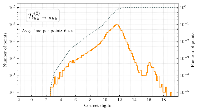
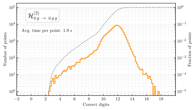
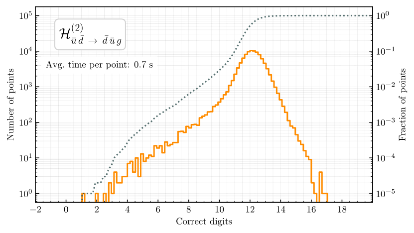
Figure 3: Distributions of the base 10 logarithm of the relative error (correct digits) of the NNLO hard functions defined in eq. 32 for representative physical channels contributing to three-jet production at hadron colliders. The dashed curves represent respective cumulative distributions. Here $N_{f}$ is set to $5$, and the renormalization scale is set dynamically to (half of) the sum of the transverse momentum of the final-state partons. The phase space definition is taken from ref. ATLAS:2014qmg.

Appendix A Reference evaluations

We present in table 4 the reference evaluations of the hard functions defined in eqs. 32 and 33 at the point

$$p_{1} =\{-3.6033749869055013,3.5549594933215615,0.033937560795432568,0.58772658529828721\},$$ (69)

$$p_{2} =\{-3.5779991067160259,3.5333697062718894,0.033731453043168395,-0.56235070510881185\},$$

$$p_{3} =\{1.7967619455543639,-1.7454551820128482,0.10779867188908804,-0.41245501926361226\},$$

$$p_{4} =\{0.41554983516150722,-0.38259279840807596,-0.13137170294301400,0.095109893149375643\},$$

$$p_{5} =\{4.9690623129056561,-4.9602812191725268,-0.044095982784675001,0.29196924592476125\},$$

with the renormalization scale set to $\mu=1$. For comparison we also show in table 5 the evaluations of the same hard functions in the leading color approximation. The evaluations are produced using the numerical code FivePointAmplitudes which we make available with this work. We remind the reader that whenever we are using the $\to$ notation, the first two particles are to be understood as crossed to be incoming.

Channel	$H^{(1)[0]}$	$H^{(1)[1]}$	$H^{(2)[0]}$	$H^{(2)[1]}$	$H^{(2)[2]}$
${\bar{u}}u\rightarrow ggg$	$-0.006212852706$	$-0.0454101007307$	$318.955641322$	$-14.6420604152$	$0.0733824569231$
${\bar{u}}g\rightarrow{\bar{u}}gg$	$39.0994013942$	$-0.492481498134$	$2066.36392385$	$-114.543895236$	$0.861580772061$
$gg\rightarrow u{\bar{u}}g$	$4.07662153685$	$0.0130905622339$	$463.236973933$	$-23.8189711025$	$-0.430932958459$
${\bar{u}}u\rightarrow d{\bar{d}}g$	$17.8776395916$	$-1.83734127116$	$552.343071009$	$-60.0556784182$	$1.52922442321$
${\bar{u}}d\rightarrow d{\bar{u}}g$	$45.4231876826$	$-1.80612761041$	$1876.8079204$	$-158.012839383$	$2.48406129185$
${\bar{u}}{\bar{d}}\rightarrow{\bar{d}}{\bar{u}}g$	$36.5463358316$	$-2.14821130255$	$1545.41004188$	$-158.008191002$	$3.32697171361$
${\bar{u}}g\rightarrow{\bar{u}}d{\bar{d}}$	$56.1144160759$	$-2.88325090618$	$2879.870086$	$-278.230078768$	$6.18882069862$
${\bar{u}}u\rightarrow u{\bar{u}}g$	$35.1251353834$	$-1.81972845991$	$1384.61457589$	$-121.556173952$	$2.13373315494$
${\bar{u}}{\bar{u}}\rightarrow{\bar{u}}{\bar{u}}g$	$71.4608675873$	$-3.67999937996$	$4392.67315319$	$-441.108685487$	$9.7657279991$
${\bar{u}}g\rightarrow{\bar{u}}u{\bar{u}}$	$54.3760288328$	$-2.83165571182$	$2801.23577819$	$-269.746150468$	$5.98133163379$

Table 4: Reference values for hard functions of each channel considered in this work, as defined in eq. 33. Here we set $N_{c}=3$.

Channel	$H^{(1)[0]}$	$H^{(1)[1]}$	$H^{(2)[0]}$	$H^{(2)[1]}$	$H^{(2)[2]}$
${\bar{u}}u\rightarrow ggg$	$-0.904169945632$	$-0.0290745413125$	$286.504396459$	$-16.4877211236$	$0.0591610370825$
${\bar{u}}g\rightarrow{\bar{u}}gg$	$35.3138994216$	$-0.491121881165$	$1709.35891402$	$-105.715888821$	$0.872329205733$
$gg\rightarrow u{\bar{u}}g$	$3.62839265602$	$0.0106464749312$	$398.255787625$	$-23.2749530656$	$-0.380163822808$
${\bar{u}}u\rightarrow d{\bar{d}}g$	$19.4220143259$	$-1.78898228361$	$568.84899353$	$-62.8383318838$	$1.40770779745$
${\bar{u}}d\rightarrow d{\bar{u}}g$	$45.7223617721$	$-1.73638756796$	$1852.5688152$	$-151.61506626$	$2.31111445374$
${\bar{u}}{\bar{d}}\rightarrow{\bar{d}}{\bar{u}}g$	$26.2821708156$	$-2.3018897729$	$1159.19990841$	$-139.532378448$	$3.70244721968$
${\bar{u}}g\rightarrow{\bar{u}}d{\bar{d}}$	$50.9489640028$	$-2.91394709477$	$2497.22216028$	$-263.212680843$	$6.36125177509$
${\bar{u}}u\rightarrow u{\bar{u}}g$	$35.8324660681$	$-1.75616511096$	$1369.84305747$	$-118.231756564$	$1.9714004014$
${\bar{u}}{\bar{u}}\rightarrow{\bar{u}}{\bar{u}}g$	$66.9539031696$	$-3.68077608088$	$3941.34122482$	$-416.819803981$	$9.78316003718$
${\bar{u}}g\rightarrow{\bar{u}}u{\bar{u}}$	$48.3172172347$	$-2.84429678497$	$2375.45809856$	$-250.314601734$	$6.06149093974$

Table 5: Reference values for hard functions in the leading color approximation of each channel considered in this work, as defined in eq. 33. Here we set $N_{c}=3$.

Appendix B Four-quark one-gluon MHV functions

$$\begin{gathered}\small\tilde{r}_{1}=\frac{{\langle}24{\rangle}}{{\langle}15{\rangle}{\langle}35{\rangle}}\end{gathered}$$	$$\begin{gathered}\small\tilde{r}_{20}=\frac{[35][25]}{{\langle}13{\rangle}[23][24]}\end{gathered}$$	$$\begin{gathered}\small\tilde{r}_{39}=\frac{{\langle}23{\rangle}^{2}[23]}{{\langle}12{\rangle}[24]{\langle}35{\rangle}^{2}}\end{gathered}$$	$$\begin{gathered}\small\tilde{r}_{58}=\frac{[13]{\langle}24{\rangle}{\langle}14{\rangle}}{{\langle}13{\rangle}[34]{\langle}45{\rangle}^{2}}\end{gathered}$$
$$\begin{gathered}\small\tilde{r}_{2}=\frac{[15]}{[24]{\langle}35{\rangle}}\end{gathered}$$	$$\begin{gathered}\small\tilde{r}_{21}=\frac{[13][25]}{[23][24]{\langle}35{\rangle}}\end{gathered}$$	$$\begin{gathered}\small\tilde{r}_{40}=\frac{{\langle}45{\rangle}[23][15]}{[12]^{2}{\langle}15{\rangle}^{2}}\end{gathered}$$	$$\begin{gathered}\small\tilde{r}_{59}=\frac{[35][13]{\langle}23{\rangle}}{{\langle}34{\rangle}[34]^{2}{\langle}35{\rangle}}\end{gathered}$$
$$\begin{gathered}\small\tilde{r}_{3}=\frac{{\langle}23{\rangle}{\langle}24{\rangle}}{{\langle}12{\rangle}{\langle}35{\rangle}^{2}}\end{gathered}$$	$$\begin{gathered}\small\tilde{r}_{22}=\frac{[35]{\langle}23{\rangle}}{{\langle}15{\rangle}{\langle}35{\rangle}[45]}\end{gathered}$$	$$\begin{gathered}\small\tilde{r}_{41}=\frac{[35]^{2}{\langle}45{\rangle}}{{\langle}12{\rangle}[23]^{2}{\langle}35{\rangle}}\end{gathered}$$	$$\begin{gathered}\small\tilde{r}_{60}=\frac{[23]{\langle}24{\rangle}{\langle}12{\rangle}}{{\langle}15{\rangle}^{2}{\langle}25{\rangle}[25]}\end{gathered}$$
$$\begin{gathered}\small\tilde{r}_{4}=\frac{{\langle}24{\rangle}^{2}}{{\langle}12{\rangle}{\langle}35{\rangle}{\langle}45{\rangle}}\end{gathered}$$	$$\begin{gathered}\small\tilde{r}_{23}=\frac{[35]{\langle}24{\rangle}}{{\langle}14{\rangle}[34]{\langle}35{\rangle}}\end{gathered}$$	$$\begin{gathered}\small\tilde{r}_{42}=\frac{[13]^{2}[25]}{[12]^{2}{\langle}15{\rangle}[34]}\end{gathered}$$	$$\begin{gathered}\small\tilde{r}_{61}=\frac{[35]^{2}{\langle}23{\rangle}}{{\langle}13{\rangle}[34]{\langle}3|1\tiny{+}2|3]}\end{gathered}$$
$$\begin{gathered}\small\tilde{r}_{5}=\frac{[12]{\langle}23{\rangle}}{[24]{\langle}35{\rangle}^{2}}\end{gathered}$$	$$\begin{gathered}\small\tilde{r}_{24}=\frac{[35]{\langle}24{\rangle}}{{\langle}14{\rangle}[24]{\langle}25{\rangle}}\end{gathered}$$	$$\begin{gathered}\small\tilde{r}_{43}=\frac{{\langle}35{\rangle}{\langle}24{\rangle}{\langle}12{\rangle}^{2}}{{\langle}15{\rangle}^{3}{\langle}23{\rangle}^{2}}\end{gathered}$$	$$\begin{gathered}\small\tilde{r}_{62}=\frac{[35]^{2}[13]}{[23][34]{\langle}3|1\tiny{+}5|3]}\end{gathered}$$
$$\begin{gathered}\small\tilde{r}_{6}=\frac{{\langle}24{\rangle}^{2}}{{\langle}13{\rangle}{\langle}25{\rangle}{\langle}45{\rangle}}\end{gathered}$$	$$\begin{gathered}\small\tilde{r}_{25}=\frac{[35]{\langle}24{\rangle}}{{\langle}15{\rangle}{\langle}34{\rangle}[34]}\end{gathered}$$	$$\begin{gathered}\small\tilde{r}_{44}=\frac{{\langle}34{\rangle}{\langle}25{\rangle}[23]^{2}}{[12]^{2}{\langle}15{\rangle}^{3}}\end{gathered}$$	$$\begin{gathered}\small\tilde{r}_{63}=\frac{{\langle}34{\rangle}[13]{\langle}23{\rangle}}{{\langle}35{\rangle}^{2}{\langle}3|1\tiny{+}5|3]}\end{gathered}$$
$$\begin{gathered}\small\tilde{r}_{7}=\frac{{\langle}23{\rangle}{\langle}45{\rangle}}{{\langle}15{\rangle}{\langle}35{\rangle}^{2}}\end{gathered}$$	$$\begin{gathered}\small\tilde{r}_{26}=\frac{[35][13]}{[14]{\langle}15{\rangle}[23]}\end{gathered}$$	$$\begin{gathered}\small\tilde{r}_{45}=\frac{{\langle}34{\rangle}^{2}[35]}{{\langle}13{\rangle}[25]{\langle}35{\rangle}{\langle}45{\rangle}}\end{gathered}$$	$$\begin{gathered}\small\tilde{r}_{64}=\frac{[14]{\langle}34{\rangle}{\langle}24{\rangle}}{{\langle}35{\rangle}^{2}{\langle}4|1\tiny{+}2|4]}\end{gathered}$$
$$\begin{gathered}\small\tilde{r}_{8}=\frac{{\langle}34{\rangle}{\langle}23{\rangle}}{{\langle}13{\rangle}{\langle}35{\rangle}^{2}}\end{gathered}$$	$$\begin{gathered}\small\tilde{r}_{27}=\frac{[35]{\langle}24{\rangle}}{{\langle}15{\rangle}{\langle}5|1\tiny{+}2|5]}\end{gathered}$$	$$\begin{gathered}\small\tilde{r}_{46}=\frac{{\langle}34{\rangle}^{2}[34]}{{\langle}13{\rangle}[24]{\langle}35{\rangle}{\langle}45{\rangle}}\end{gathered}$$	$$\begin{gathered}\small\tilde{r}_{65}=\frac{[35]^{2}{\langle}25{\rangle}}{{\langle}15{\rangle}[34]{\langle}5|1\tiny{+}2|5]}\end{gathered}$$
$$\begin{gathered}\small\tilde{r}_{9}=\frac{{\langle}23{\rangle}[15]}{{\langle}35{\rangle}^{2}[45]}\end{gathered}$$	$$\begin{gathered}\small\tilde{r}_{28}=\frac{{\langle}24{\rangle}^{3}}{{\langle}12{\rangle}{\langle}25{\rangle}{\langle}34{\rangle}{\langle}45{\rangle}}\end{gathered}$$	$$\begin{gathered}\small\tilde{r}_{47}=\frac{{\langle}34{\rangle}[35]{\langle}14{\rangle}}{{\langle}13{\rangle}^{2}[23]{\langle}45{\rangle}}\end{gathered}$$	$$\begin{gathered}\small\tilde{r}_{66}=\frac{[15]^{2}{\langle}14{\rangle}}{[25]{\langle}35{\rangle}{\langle}5|1\tiny{+}2|5]}\end{gathered}$$
$$\begin{gathered}\small\tilde{r}_{10}=\frac{[13]{\langle}23{\rangle}}{[34]{\langle}35{\rangle}^{2}}\end{gathered}$$	$$\begin{gathered}\small\tilde{r}_{29}=\frac{{\langle}45{\rangle}[23]{\langle}12{\rangle}}{[12]{\langle}15{\rangle}^{3}}\end{gathered}$$	$$\begin{gathered}\small\tilde{r}_{48}=\frac{[35]{\langle}24{\rangle}^{2}}{{\langle}14{\rangle}{\langle}25{\rangle}{\langle}45{\rangle}[45]}\end{gathered}$$	$$\begin{gathered}\small\tilde{r}_{67}=\frac{[35]{\langle}25{\rangle}{\langle}14{\rangle}}{{\langle}15{\rangle}^{2}{\langle}5|1\tiny{+}2|5]}\end{gathered}$$
$$\begin{gathered}\small\tilde{r}_{11}=\frac{[45][23]}{{\langle}15{\rangle}[24]^{2}}\end{gathered}$$	$$\begin{gathered}\small\tilde{r}_{30}=\frac{{\langle}23{\rangle}{\langle}24{\rangle}{\langle}12{\rangle}}{{\langle}13{\rangle}^{2}{\langle}25{\rangle}^{2}}\end{gathered}$$	$$\begin{gathered}\small\tilde{r}_{49}=\frac{[45]{\langle}24{\rangle}^{2}}{{\langle}15{\rangle}{\langle}23{\rangle}{\langle}25{\rangle}[25]}\end{gathered}$$	$$\begin{gathered}\small\tilde{r}_{68}=\frac{[35]{\langle}24{\rangle}^{2}}{{\langle}12{\rangle}{\langle}45{\rangle}{\langle}4|1\tiny{+}2|4]}\end{gathered}$$
$$\begin{gathered}\small\tilde{r}_{12}=\frac{[35]^{2}}{{\langle}13{\rangle}[23][34]}\end{gathered}$$	$$\begin{gathered}\small\tilde{r}_{31}=\frac{[13]^{2}{\langle}12{\rangle}}{[34]^{2}{\langle}35{\rangle}{\langle}45{\rangle}}\end{gathered}$$	$$\begin{gathered}\small\tilde{r}_{50}=\frac{{\langle}45{\rangle}{\langle}23{\rangle}[15]}{{\langle}12{\rangle}[12]{\langle}35{\rangle}^{2}}\end{gathered}$$	$$\begin{gathered}\small\tilde{r}_{69}=\frac{{\langle}34{\rangle}[13]{\langle}23{\rangle}}{{\langle}35{\rangle}^{2}{\langle}3|1\tiny{+}2|3]}\end{gathered}$$
$$\begin{gathered}\small\tilde{r}_{13}=\frac{[15]^{2}}{[12]{\langle}35{\rangle}[45]}\end{gathered}$$	$$\begin{gathered}\small\tilde{r}_{32}=\frac{[15]^{2}{\langle}12{\rangle}}{{\langle}35{\rangle}{\langle}45{\rangle}[45]^{2}}\end{gathered}$$	$$\begin{gathered}\small\tilde{r}_{51}=\frac{[13]^{2}{\langle}23{\rangle}}{[12]{\langle}25{\rangle}[34]{\langle}35{\rangle}}\end{gathered}$$	$$\begin{gathered}\small\tilde{r}_{70}=\frac{[35]{\langle}35{\rangle}{\langle}12{\rangle}^{2}}{{\langle}15{\rangle}^{3}{\langle}23{\rangle}[45]}\end{gathered}$$
$$\begin{gathered}\small\tilde{r}_{14}=\frac{[23]{\langle}24{\rangle}}{[12]{\langle}15{\rangle}^{2}}\end{gathered}$$	$$\begin{gathered}\small\tilde{r}_{33}=\frac{[45]{\langle}14{\rangle}^{2}}{{\langle}13{\rangle}^{2}{\langle}15{\rangle}[23]}\end{gathered}$$	$$\begin{gathered}\small\tilde{r}_{52}=\frac{[15]{\langle}24{\rangle}^{2}}{{\langle}12{\rangle}[14]{\langle}34{\rangle}{\langle}45{\rangle}}\end{gathered}$$	$$\begin{gathered}\small\tilde{r}_{71}=\frac{{\langle}34{\rangle}^{2}[34]{\langle}45{\rangle}}{{\langle}14{\rangle}[23]{\langle}35{\rangle}^{3}}\end{gathered}$$
$$\begin{gathered}\small\tilde{r}_{15}=\frac{{\langle}34{\rangle}^{2}{\langle}25{\rangle}}{{\langle}14{\rangle}{\langle}35{\rangle}^{3}}\end{gathered}$$	$$\begin{gathered}\small\tilde{r}_{34}=\frac{{\langle}23{\rangle}{\langle}14{\rangle}^{2}}{{\langle}13{\rangle}^{2}{\langle}15{\rangle}{\langle}45{\rangle}}\end{gathered}$$	$$\begin{gathered}\small\tilde{r}_{53}=\frac{[13]{\langle}24{\rangle}^{2}}{{\langle}12{\rangle}[12]{\langle}25{\rangle}{\langle}45{\rangle}}\end{gathered}$$	$$\begin{gathered}\small\tilde{r}_{72}=\frac{{\langle}34{\rangle}[13]^{2}[15]}{{\langle}12{\rangle}[12]^{3}{\langle}25{\rangle}}\end{gathered}$$
$$\begin{gathered}\small\tilde{r}_{16}=\frac{[12]{\langle}24{\rangle}}{[24]{\langle}35{\rangle}{\langle}45{\rangle}}\end{gathered}$$	$$\begin{gathered}\small\tilde{r}_{35}=\frac{[14]{\langle}24{\rangle}^{2}}{[24]{\langle}25{\rangle}^{2}{\langle}34{\rangle}}\end{gathered}$$	$$\begin{gathered}\small\tilde{r}_{54}=\frac{[25]{\langle}24{\rangle}^{2}}{{\langle}12{\rangle}[24]{\langle}34{\rangle}{\langle}45{\rangle}}\end{gathered}$$	$$\begin{gathered}\small\tilde{r}_{73}=\frac{{\langle}34{\rangle}[35]^{2}{\langle}25{\rangle}[15]}{{\langle}5|1\tiny{+}2|5]^{3}}\end{gathered}$$
$$\begin{gathered}\small\tilde{r}_{17}=\frac{{\langle}23{\rangle}{\langle}24{\rangle}}{{\langle}13{\rangle}{\langle}25{\rangle}{\langle}35{\rangle}}\end{gathered}$$	$$\begin{gathered}\small\tilde{r}_{36}=\frac{[13]{\langle}24{\rangle}^{2}}{[23]{\langle}25{\rangle}^{2}{\langle}34{\rangle}}\end{gathered}$$	$$\begin{gathered}\small\tilde{r}_{55}=\frac{{\langle}34{\rangle}[13][15]}{[12]{\langle}35{\rangle}^{2}[35]}\end{gathered}$$	$$\begin{gathered}\small\tilde{r}_{74}=\frac{[35][15]^{2}{\langle}14{\rangle}}{[25]{\langle}5|1\tiny{+}2|5]^{2}}\end{gathered}$$
$$\begin{gathered}\small\tilde{r}_{18}=\frac{[15]{\langle}24{\rangle}}{{\langle}35{\rangle}{\langle}45{\rangle}[45]}\end{gathered}$$	$$\begin{gathered}\small\tilde{r}_{37}=\frac{{\langle}23{\rangle}[23]^{2}}{[12]{\langle}15{\rangle}^{2}[24]}\end{gathered}$$	$$\begin{gathered}\small\tilde{r}_{56}=\frac{[15]^{2}{\langle}14{\rangle}}{{\langle}13{\rangle}[13][24]{\langle}34{\rangle}}\end{gathered}$$	$$\begin{gathered}\small\tilde{r}_{75}=\frac{[35]{\langle}45{\rangle}[15]^{2}}{[12]{\langle}5|1\tiny{+}2|5]^{2}}\end{gathered}$$
$$\begin{gathered}\small\tilde{r}_{19}=\frac{[13]{\langle}24{\rangle}}{[34]{\langle}35{\rangle}{\langle}45{\rangle}}\end{gathered}$$	$$\begin{gathered}\small\tilde{r}_{38}=\frac{[13]{\langle}23{\rangle}^{2}}{{\langle}12{\rangle}[14]{\langle}35{\rangle}^{2}}\end{gathered}$$	$$\begin{gathered}\small\tilde{r}_{57}=\frac{[35]^{2}{\langle}24{\rangle}}{{\langle}12{\rangle}{\langle}13{\rangle}[13][23]}\end{gathered}$$	$$\begin{gathered}\small\tilde{r}_{76}=\frac{[45][12]{\langle}24{\rangle}^{2}}{{\langle}35{\rangle}{\langle}4|1\tiny{+}2|4]^{2}}\end{gathered}$$

$$\begin{gathered}\small\tilde{r}_{77}=\frac{{\langle}25{\rangle}^{2}[15]^{2}}{{\langle}12{\rangle}[14]^{2}{\langle}35{\rangle}{\langle}45{\rangle}}\end{gathered}$$	$$\begin{gathered}\small\tilde{r}_{96}=\frac{[35]^{2}[12]{\langle}12{\rangle}}{{\langle}15{\rangle}{\langle}25{\rangle}[25]^{2}[34]}\end{gathered}$$	$$\begin{gathered}\small\tilde{r}_{115}=\frac{[34]{\langle}12{\rangle}[23]{\langle}34{\rangle}{\langle}45{\rangle}}{[12]{\langle}15{\rangle}^{3}{\langle}25{\rangle}[25]}\end{gathered}$$
$$\begin{gathered}\small\tilde{r}_{78}=\frac{[13]^{2}{\langle}23{\rangle}^{2}}{{\langle}12{\rangle}[14]^{2}{\langle}35{\rangle}{\langle}45{\rangle}}\end{gathered}$$	$$\begin{gathered}\small\tilde{r}_{97}=\frac{[35]{\langle}13{\rangle}{\langle}24{\rangle}^{2}}{{\langle}12{\rangle}^{2}[25]{\langle}35{\rangle}{\langle}45{\rangle}}\end{gathered}$$	$$\begin{gathered}\small\tilde{r}_{116}=\frac{{\langle}25{\rangle}[24][35]{\langle}45{\rangle}{\langle}23{\rangle}}{{\langle}15{\rangle}[34]{\langle}35{\rangle}^{2}{\langle}5|1\tiny{+}2|5]}\end{gathered}$$
$$\begin{gathered}\small\tilde{r}_{79}=\frac{[25]^{2}{\langle}25{\rangle}^{2}}{{\langle}12{\rangle}[24]^{2}{\langle}35{\rangle}{\langle}45{\rangle}}\end{gathered}$$	$$\begin{gathered}\small\tilde{r}_{98}=\frac{[25]^{2}{\langle}23{\rangle}{\langle}12{\rangle}}{{\langle}13{\rangle}^{2}[24]{\langle}2|1\tiny{+}3|2]}\end{gathered}$$	$$\begin{gathered}\small\tilde{r}_{117}=\frac{[35]^{3}{\langle}45{\rangle}{\langle}25{\rangle}{\langle}13{\rangle}}{{\langle}12{\rangle}{\langle}14{\rangle}[23]{\langle}34{\rangle}[34]^{2}{\langle}35{\rangle}}\end{gathered}$$
$$\begin{gathered}\small\tilde{r}_{80}=\frac{[14]^{2}{\langle}14{\rangle}^{2}}{{\langle}12{\rangle}[24]^{2}{\langle}35{\rangle}{\langle}45{\rangle}}\end{gathered}$$	$$\begin{gathered}\small\tilde{r}_{99}=\frac{[35]^{3}[13]{\langle}23{\rangle}{\langle}35{\rangle}}{[34]{\langle}3|1\tiny{+}2|3]^{3}}\end{gathered}$$	$$\begin{gathered}\small\tilde{r}_{118}=\frac{[45]^{2}{\langle}45{\rangle}^{2}}{{\langle}15{\rangle}[24]{\langle}34{\rangle}[34]{\langle}35{\rangle}}+\\ \small\frac{-2{\langle}24{\rangle}[45]{\langle}45{\rangle}}{{\langle}15{\rangle}{\langle}34{\rangle}[34]{\langle}35{\rangle}}\phantom{+}\end{gathered}$$
$$\begin{gathered}\small\tilde{r}_{81}=\frac{{\langle}23{\rangle}[15]{\langle}14{\rangle}}{{\langle}13{\rangle}{\langle}35{\rangle}{\langle}45{\rangle}[45]}\end{gathered}$$	$$\begin{gathered}\small\tilde{r}_{100}=\frac{[14]^{2}{\langle}14{\rangle}^{3}}{{\langle}12{\rangle}{\langle}15{\rangle}[24]^{2}{\langle}34{\rangle}{\langle}45{\rangle}}\end{gathered}$$	$$\begin{gathered}\small\tilde{r}_{119}=\frac{3{\langle}35{\rangle}{\langle}12{\rangle}[35]^{2}[15]^{2}{\langle}45{\rangle}}{{\langle}5|1\tiny{+}2|5]^{4}}+\\ \small\frac{-2[35]^{2}{\langle}35{\rangle}[15]{\langle}24{\rangle}}{{\langle}5|1\tiny{+}2|5]^{3}}\phantom{+}\end{gathered}$$
$$\begin{gathered}\small\tilde{r}_{82}=\frac{[25]{\langle}23{\rangle}{\langle}24{\rangle}}{{\langle}12{\rangle}[24]{\langle}34{\rangle}{\langle}35{\rangle}}\end{gathered}$$	$$\begin{gathered}\small\tilde{r}_{101}=\frac{[35]^{2}[13]^{2}{\langle}13{\rangle}}{[23][34]{\langle}3|1\tiny{+}2|3]^{2}}\end{gathered}$$	$$\begin{gathered}\small\tilde{r}_{120}=\frac{[45]^{2}{\langle}45{\rangle}^{2}{\langle}25{\rangle}}{{\langle}15{\rangle}{\langle}34{\rangle}[34]^{2}{\langle}35{\rangle}^{2}}+\\ \small\frac{2[45]{\langle}45{\rangle}{\langle}24{\rangle}}{{\langle}15{\rangle}{\langle}34{\rangle}[34]{\langle}35{\rangle}}\phantom{+}\end{gathered}$$
$$\begin{gathered}\small\tilde{r}_{83}=\frac{[13]{\langle}23{\rangle}{\langle}24{\rangle}}{{\langle}13{\rangle}[14]{\langle}25{\rangle}{\langle}45{\rangle}}\end{gathered}$$	$$\begin{gathered}\small\tilde{r}_{102}=\frac{{\langle}23{\rangle}[15]{\langle}24{\rangle}{\langle}14{\rangle}}{{\langle}12{\rangle}[24]{\langle}25{\rangle}{\langle}34{\rangle}^{2}}\end{gathered}$$	$$\begin{gathered}\small\tilde{r}_{121}=\frac{-3[13]^{2}[25]^{2}{\langle}25{\rangle}}{{\langle}12{\rangle}[12]^{3}{\langle}15{\rangle}[34]}+\\ \small\frac{2{\langle}45{\rangle}^{2}[25][15][34]}{{\langle}12{\rangle}[12]^{3}{\langle}15{\rangle}^{2}}+\\ \small\frac{3{\langle}34{\rangle}[13][35]}{{\langle}12{\rangle}[12]^{2}{\langle}15{\rangle}}\phantom{+}\end{gathered}$$
$$\begin{gathered}\small\tilde{r}_{84}=\frac{[25]{\langle}23{\rangle}{\langle}24{\rangle}}{{\langle}12{\rangle}[12]{\langle}13{\rangle}{\langle}35{\rangle}}\end{gathered}$$	$$\begin{gathered}\small\tilde{r}_{103}=\frac{{\langle}45{\rangle}[34]{\langle}13{\rangle}{\langle}24{\rangle}}{{\langle}14{\rangle}[14]{\langle}15{\rangle}^{2}{\langle}35{\rangle}}\end{gathered}$$	$$\begin{gathered}\small\tilde{r}_{122}=\frac{{\langle}24{\rangle}[23]{\langle}2|1\tiny{+}5|2]}{{\langle}12{\rangle}[12]^{2}{\langle}15{\rangle}^{2}}+\\ \small\frac{-2[35]{\langle}2|1\tiny{+}5|2]{\langle}14{\rangle}}{{\langle}12{\rangle}[12]{\langle}15{\rangle}^{2}[25]}+\\ \small\frac{2{\langle}2|1\tiny{+}5|2][23]{\langle}25{\rangle}{\langle}45{\rangle}[25]}{{\langle}12{\rangle}[12]^{3}{\langle}15{\rangle}^{3}}\phantom{+}\end{gathered}$$