$\mathbb{Z}_{2}\times\mathbb{Z}_{2}$ Equivariant Quantum Neural Networks: Benchmarking against Classical Neural Networks

Abstract

This paper presents a comprehensive comparative analysis of the performance of Equivariant Quantum Neural Networks (EQNN) and Quantum Neural Networks (QNN), juxtaposed against their classical counterparts: Equivariant Neural Networks (ENN) and Deep Neural Networks (DNN). We evaluate the performance of each network with two toy examples for a binary classification task, focusing on model complexity (measured by the number of parameters) and the size of the training data set. Our results show that the $\mathbb{Z}_{2}\times\mathbb{Z}_{2}$ EQNN and the QNN provide superior performance for smaller parameter sets and modest training data samples.

1 Introduction

Classical Equivariant Neural Networks (ENNs) exploit the underlying symmetry structure of the data, ensuring that the input and output transform consistently under the symmetry [1]. ENNs have been widely used in various applications including deep convolutional neural networks for computer vision [2], AlphaFold for protein structure prediction [3], Lorentz equivariant neural networks for particle physics [4], etc. In recent years, significant development has been made in their quantum counterparts, Equivariant Quantum Neural Networks (EQNNs) [5, 6, 7, 8].

In this paper we benchmark the performance of EQNNs against various classical and/or non-equivariant alternatives for two-dimensional toy data sets, which exhibit a $\mathbb{Z}_{2}\times\mathbb{Z}_{2}$ symmetry structure. Such patterns often appear in high-energy physics data, e.g., as kinematic boundaries in the high-dimensional phase space describing the final state [9, 10]. By a clever choice of the kinematic variables for the analysis, these boundaries can be preserved in projections onto a lower-dimensional feature space [11, 12, 13, 14, 15]. In this study, we consider simplified two-dimensional data sets that mimic the data arising in such projections.

2 Dataset Description

In both examples, we consider two-dimensional data $(x_{1},x_{2})$ on the unit square ($-1\leq x_{i}\leq 1$) (see Fig. 1). The data points belong to two classes: $y=+1$ (blue points) and $y=-1$ (red points). In the first example (left panel of Fig. 1), the labels are generated by the function

$$y(x_{1},x_{2})=2H\left(R-\sqrt{(x_{1}+1)^{2}+(x_{2}-1)^{2}}\right)+2H\left(R-\sqrt{(x_{1}-1)^{2}+(x_{2}+1)^{2}}\right)-1,$$ (1)

where $H(x)$ is the Heaviside step function and for definiteness we choose $R=1.1$. The function (1) respects a $\mathbb{Z}_{2}\times\mathbb{Z}_{2}$ symmetry, where the first $\mathbb{Z}_{2}$ is given by a reflection about the $x_{1}=x_{2}$ diagonal

$$x_{1}\to x_{2},\qquad x_{2}\to x_{1},\qquad y\to y,$$ (2)

while the second $\mathbb{Z}_{2}$ corresponds to a reflection about the $x_{1}=-x_{2}$ diagonal

$$x_{1}\to-x_{2},\qquad x_{2}\to-x_{1},\qquad y\to y.$$ (3)

This $\mathbb{Z}_{2}\times\mathbb{Z}_{2}$ example was studied in Ref. [6] and we shall refer to it as the symmetric case, since the $y$ label is invariant.

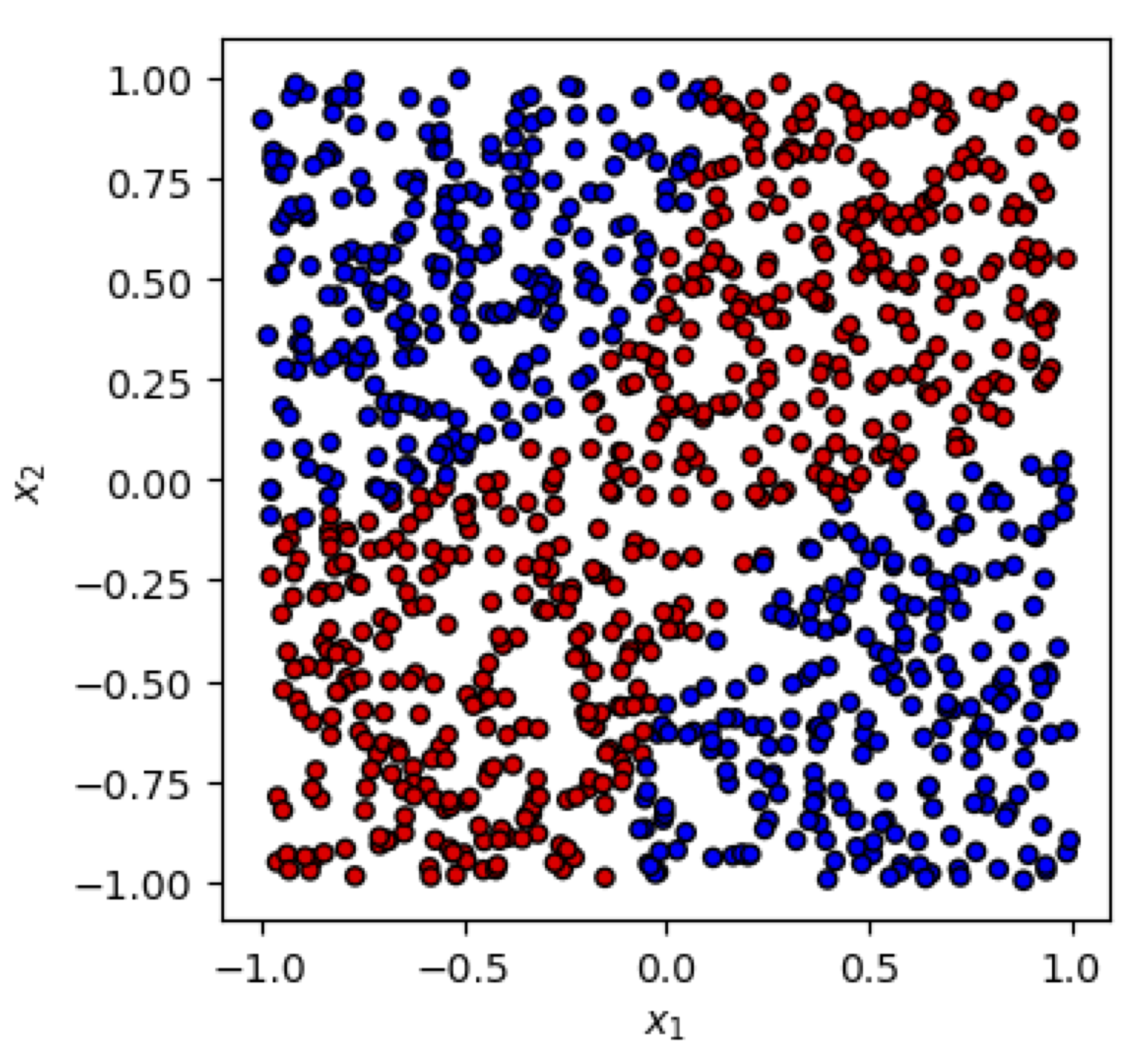
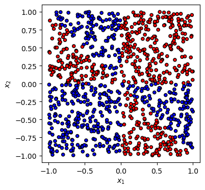
Figure 1: Pictorial illustration of the datasets used in this study - the symmetric case (1) in the left panel and the anti-symmetric case (4) in the right panel.

The second example is illustrated in the right panel of Fig. 1. The labels are generated by the function

$$y(x_{1},x_{2}) =H\left(-x_{1}\right)H\left(-x_{2}\right)+H\left(-x_{1}\right)H\left(x_{2}\right)H(x_{1}+x_{2})$$

$$-H\left(x_{1}\right)H\left(x_{2}\right)+H\left(x_{1}\right)H\left(-x_{2}\right)H(x_{1}+x_{2}).$$ (4)

The first $\mathbb{Z}_{2}$ is still realized as in (2). However, this time the labels are flipped under a reflection along the $x_{1}=-x_{2}$ diagonal:

$$x_{1}\to-x_{2},\qquad x_{2}\to-x_{1},\qquad y\to-y,$$ (5)

which is why we shall refer to this case as anti-symmetric.

3 Network Architectures

To assess the importance of embedding the symmetry in the network, and to compare the classical and quantum versions of the networks, we study the performance of the following four different architectures: (i) Deep Neural Network (DNN), (ii) Equivariant Neural Network (ENN), (iii) Quantum Neural Network (QNN), and (iv) Equivariant Quantum Neural Network (EQNN). In each case, we adjust the hyperparameters to ensure that the number of network parameters is roughly the same.

Deep Neural Networks. In our DNN, for the symmetric (anti-symmetric) case we use 1 (2) hidden layer(s) with 4 neurons. For both types of classical networks, we use softmax activation function, Adam optimizer and learning rate of $0.1$. We use the binary cross entropy for both DNN and ENN.

Equivariant Neural Networks. A given map $f:x\in X\to f(x)\in Y$ between an input space $X$ and an output space $Y$ is said to be equivariant under a group $G$ if it satisfies the following relation:

$$f(g_{\text{in}}(x))=g_{\text{out}}(f(x)),$$ (6)

where $g_{\text{in}}$ ($g_{\text{out}}$) is a representation of a group element $g\in G$ acting on the input (output) space. In the special case when $g_{\text{out}}$ is the trivial representation, the map is called invariant under the group $G$, i.e. a symmetry transformation acting on the input data $x$ does not change the output of the map. The goal of ENNs, or equivariant learning models in general, is to design a trainable map $f$ which would always satisfy Eq. (6). In tasks where the symmetry is known, such equivariant models are believed to have an advantage in terms of number of parameters and training complexity. Several studies in high-energy physics have attempted to use classical equivariant neural networks [4, 16, 17, 18, 19]. Our ENN model utilizes four $\mathbb{Z}_{2}\times\mathbb{Z}_{2}$ symmetric copies for each data point, which are fed into the input layer, followed by one equivariant layer with 3 (2) neurons and one dense layer with 4 (4) neurons in the symmetric (anti-symmetric) case.

Quantum Neural Networks. For QNN, we utilize the one-qubit data-reuploading model [20] with depth four (eight) for the symmetric (anti-symmetric) case, using the angle embedding and $3$ parameters at each depth. This choice leads to a similar number of parameters as in the classical networks. We use the Adam optimizer and the loss

$$L_{QNN}=y(1-|\mathinner{\langle{\psi}|}O_{1}\mathinner{|{\psi}\rangle}|)^{2}+(1-y)(1-|\mathinner{\langle{\psi}|}O_{2}\mathinner{|{\psi}\rangle}|)^{2}$$ (7)

for any choice of two orthogonal operators $O_{1}$ and $O_{2}$ (see Ref. [21] for more details.). In this paper, we use

$$O_{1}=\dfrac{1}{4}\begin{pmatrix}[r]1&1&1&-1\\ 1&1&1&-1\\ 1&1&1&-1\\ -1&-1&-1&1\end{pmatrix},\quad\quad O_{2}=\dfrac{1}{4}\begin{pmatrix}[r]1&-1&-1&-1\\ -1&1&1&1\\ -1&1&1&1\\ -1&1&1&1\end{pmatrix}.$$ (8)

Equivariant Quantum Neural Networks. In EQNN models symmetry transformations acting on the embedding space of input features are realized as finite-dimensional unitary transformations $U_{g}$, $g\in G$. Consider the simplest case where one trainable operator $U(\theta,x)$ acts on a state $\mathinner{|{\psi}\rangle}$: $U(\theta,x)\mathinner{|{\psi}\rangle}$. If for a symmetry transformation $U_{g}$, the condition

$$U(\theta,x)\,U_{g}\mathinner{|{\psi}\rangle}=U_{g}\,U(\theta,x)\mathinner{|{\psi}\rangle},$$ (9)

is satisfied, then the operator $U$ is equivariant, i.e., the equivariant gate should commute with the symmetry. In general, the $U_{g}$ operators on the two sides of Eq. (9) do not necessarily have to be in the same representation, but are often assumed so for simplicity. The output of a QNN is the measurement of the expectation value of the state with respect to some observable $O$. If the gates are equivariant and we apply some symmetry transformation $U_{g}$, then this is equivalent to measuring the observable $U_{g}^{\dagger}OU_{g}$. Hence if $O$ commutes with the symmetry $U_{g}$, the model as a whole would be invariant under $U_{g}$, which is the case in our symmetric example. Otherwise the model is equivariant, as in our anti-symmetric example.

Our EQNN uses the two-qubit quantum circuit depicted in Fig. 2. The two $R_{Z}$ gates embed $x_{1}$ and $x_{2}$, respectively. The $R_{X}$ gates share the same parameter ($\theta_{1}$) and the $R_{ZZ}$ gate uses another parameter ($\theta_{2}$). The invariant model (for the symmetric case) uses the same observable ${O}$ for both classes in the data. In the anti-symmetric case we use two different observables ${O}_{1}$ and ${O}_{2}$ that correspond to each label. They transform into one another under reflection $g_{r}$, i.e., $U^{\dagger}_{g_{r}}{O}_{1}U_{g_{r}}={O}_{2}$. In the symmetric case we use binary cross-entropy loss, assuming the true label $y$ is either $0$ or $1$,

$$L_{EQNN}=y\log\Big{(}\mathinner{\langle{\psi}|}O\mathinner{|{\psi}\rangle}\Big{)}+(1-y)\log\Big{(}1-\mathinner{\langle{\psi}|}O\mathinner{|{\psi}\rangle}\Big{)}\,.$$ (10)

In the anti-symmetric case we used the same loss as in QNN where $O_{1}$ ($O_{2}$) is the observable corresponding to $y=1$ ($y=0$). The observables $O$ and the reflection $U_{g_{r}}$ along $x_{1}=-x_{2}$ are defined as follows:

$$O=\dfrac{1}{4}\begin{pmatrix}1&1&1&1\\ 1&1&1&1\\ 1&1&1&1\\ 1&1&1&1\end{pmatrix},\quad\quad U_{g_{r}}=\begin{pmatrix}0&0&0&1\\ 0&0&1&0\\ 0&1&0&0\\ 1&0&0&0\end{pmatrix}.$$ (11)

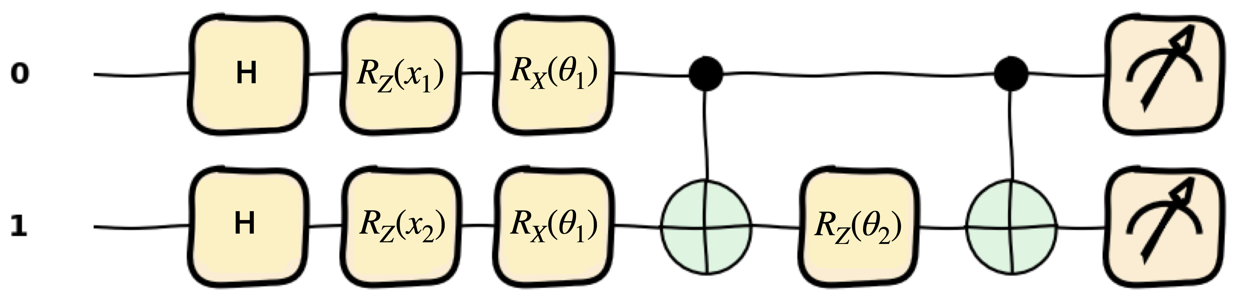
Figure 2: Illustration of the quantum circuit used for EQNN at depth 1. This circuit is repeated five (ten) times with different parameters for the symmetric (anti-symmetric) case.

4 Results

Fig. 3 shows receiver operating characteristic (ROC) curves for each network with $N_{\rm train}=200$ and $N_{\rm test}=2000$ samples for the symmetric (left) and anti-symmetric (right) dataset. As expected, networks with equivariance structure (EQNN and ENN) improve the performance of the corresponding networks (QNN and DNN) without the symmetry. We also observe that quantum networks perform better than the classical analogs. In the legends, numerical values followed by network acronyms represent the number of parameters used for each network. For the symmetric example, EQNN uses only 10 parameters, thus for fair comparison we constructed the other networks with ${\cal O}$(10) parameters as well. For the anti-symmetric example, we use 20 parameters for the EQNN. The evolution of the accuracy during training is shown in Fig. 4. The accuracy converges faster (after only 5 epochs) for QNN and EQNN in comparison to their classical counterparts (10-20 epochs).

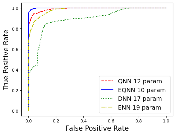
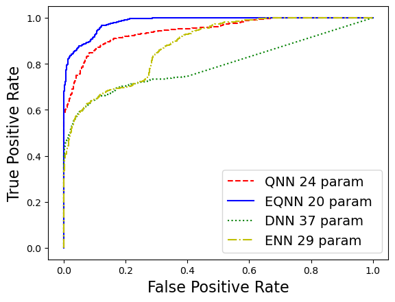
Figure 3: ROC curves for the symmetric (left) and anti-symmetric (right) example.

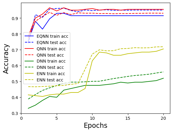
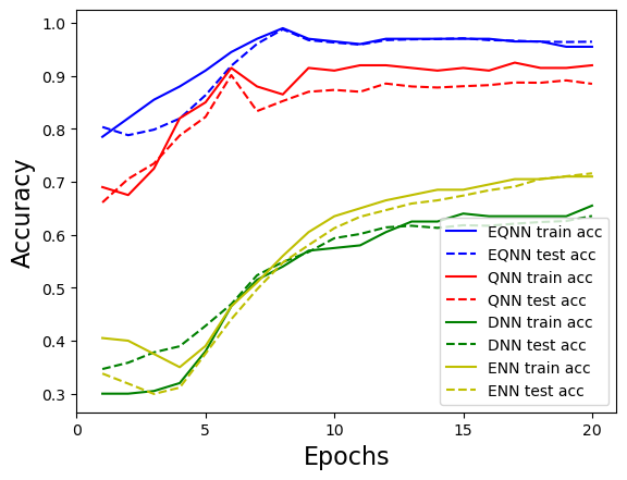
Figure 4: Accuracies during training for the symmetric (left) and anti-symmetric (right) example.

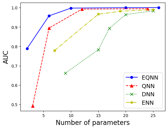
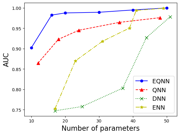
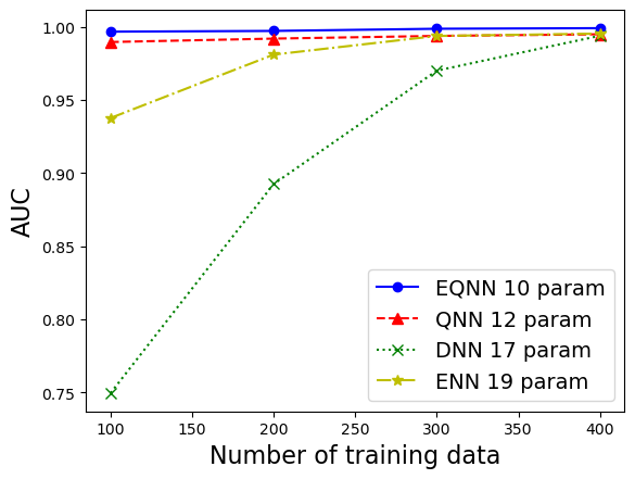
Figure 5: AUC as a function of the number of parameters (top) for fixed $N_{\rm train}=2000$ and $N_{\rm test}=200$, and as a function of $N_{\rm train}$ (bottom) with a fixed number of parameters as shown in the legend. The left (right) panels show results for the symmetric (anti-symmetric) example.

To further quantify the performance of our quantum networks, in Fig. 5 we show AUC (Area under the ROC Curve) as a function of the number of parameters (top panels) with a fixed size of the training data ($N_{\rm train}=200$), and as a function of the number of training samples (bottom panels) with a fixed number of parameters ($N_{\rm params}=20$). The left (right) panels show results for the symmetric (anti-symmetric) dataset. As the number of parameters increases, the performance of all networks improves. All AUC values become similar when $N_{\rm params}\approx 20$ ($N_{\rm params}\approx 40$) for the symmetric (anti-symmetric) case. As shown in the bottom panels, the performances of all networks become comparable to each other for both examples, once the size of the training data reaches $\sim 400$.

5 Conclusion

Our study demonstrates that EQNNs and QNNs outperform their classical counterparts, particularly in scenarios with fewer parameters and smaller training datasets. This highlights the potential of quantum-inspired architectures in resource-constrained settings. The code used for this study is publicly available at https://github.com/ZhongtianD/EQNN/tree/main.

Acknowledgements: KM is supported in part by the U.S. Department of Energy award number DE-SC0022148. KK is supported in parts by US DOE DE-SC0024407. CD is supported in part by College of Liberal Arts and Sciences Research Fund at the University of Kansas. This research used resources of the National Energy Research Scientific Computing Center, a DOE Office of Science User Facility supported by the Office of Science of the U.S. Department of Energy under Contract No. DE-AC02-05CH11231 using NERSC award NERSC DDR-ERCAP0025759. SG is supported in part by the U.S. Department of Energy (DOE) under Award No. DE-SC0012447. CD, RF, EU, MCC and TM were participants in the 2023 Google Summer of Code.

References

- Cohen and Welling [2016] Taco Cohen and Max Welling. Group equivariant convolutional networks. In Maria Florina Balcan and Kilian Q. Weinberger, editors, Proceedings of The 33rd International Conference on Machine Learning, volume 48 of Proceedings of Machine Learning Research, pages 2990–2999, New York, New York, USA, 20–22 Jun 2016. PMLR. URL https://proceedings.mlr.press/v48/cohenc16.html.
- Krizhevsky et al. [2012] Alex Krizhevsky, Ilya Sutskever, and Geoffrey E Hinton. Imagenet classification with deep convolutional neural networks. In F. Pereira, C.J. Burges, L. Bottou, and K.Q. Weinberger, editors, Advances in Neural Information Processing Systems, volume 25. Curran Associates, Inc., 2012. URL https://proceedings.neurips.cc/paper_files/paper/2012/file/c399862d3b9d6b76c8436e924a68c45b-Paper.pdf.
- Jumper et al. [2021] John M. Jumper, Richard Evans, Alexander Pritzel, Tim Green, Michael Figurnov, Olaf Ronneberger, Kathryn Tunyasuvunakool, Russ Bates, Augustin Zídek, Anna Potapenko, Alex Bridgland, Clemens Meyer, Simon A A Kohl, Andy Ballard, Andrew Cowie, Bernardino Romera-Paredes, Stanislav Nikolov, Rishub Jain, Jonas Adler, Trevor Back, Stig Petersen, David A. Reiman, Ellen Clancy, Michal Zielinski, Martin Steinegger, Michalina Pacholska, Tamas Berghammer, Sebastian Bodenstein, David Silver, Oriol Vinyals, Andrew W. Senior, Koray Kavukcuoglu, Pushmeet Kohli, and Demis Hassabis. Highly accurate protein structure prediction with alphafold. Nature, 596:583 – 589, 2021. URL https://api.semanticscholar.org/CorpusID:235959867.
- Bogatskiy et al. [2020] Alexander Bogatskiy, Brandon Anderson, Jan Offermann, Marwah Roussi, David Miller, and Risi Kondor. Lorentz group equivariant neural network for particle physics. In Hal Daumé III and Aarti Singh, editors, Proceedings of the 37th International Conference on Machine Learning, volume 119 of Proceedings of Machine Learning Research, pages 992–1002. PMLR, 13–18 Jul 2020. URL https://proceedings.mlr.press/v119/bogatskiy20a.html.
- Nguyen et al. [2022] Quynh T. Nguyen, Louis Schatzki, Paolo Braccia, Michael Ragone, Patrick J. Coles, Frederic Sauvage, Martin Larocca, and M. Cerezo. Theory for equivariant quantum neural networks, 2022.
- Meyer et al. [2023] Johannes Jakob Meyer, Marian Mularski, Elies Gil-Fuster, Antonio Anna Mele, Francesco Arzani, Alissa Wilms, and Jens Eisert. Exploiting symmetry in variational quantum machine learning. PRX Quantum, 4(1), mar 2023. doi: 10.1103/prxquantum.4.010328. URL https://doi.org/10.1103%2Fprxquantum.4.010328.
- West et al. [2023] Maxwell T West, Martin Sevior, and Muhammad Usman. Reflection equivariant quantum neural networks for enhanced image classification. Machine Learning: Science and Technology, 4(3):035027, aug 2023. doi: 10.1088/2632-2153/acf096. URL https://doi.org/10.1088%2F2632-2153%2Facf096.
- Skolik et al. [2023] Andrea Skolik, Michele Cattelan, Sheir Yarkoni, Thomas Bäck, and Vedran Dunjko. Equivariant quantum circuits for learning on weighted graphs. npj Quantum Information, 9(1):47, 2023.
- Kim [2010] Ian-Woo Kim. Algebraic Singularity Method for Mass Measurement with Missing Energy. Phys. Rev. Lett., 104:081601, 2010. doi: 10.1103/PhysRevLett.104.081601.
- Franceschini et al. [2022] Roberto Franceschini, Doojin Kim, Kyoungchul Kong, Konstantin T. Matchev, Myeonghun Park, and Prasanth Shyamsundar. Kinematic Variables and Feature Engineering for Particle Phenomenology. Reviews of Modern Physics, 6 2022.
- Kersting [2009] N. Kersting. On Measuring Split-SUSY Gaugino Masses at the LHC. Eur. Phys. J. C, 63:23–32, 2009. doi: 10.1140/epjc/s10052-009-1063-6.
- Bisset et al. [2011] M. Bisset, R. Lu, and N. Kersting. Improving SUSY Spectrum Determinations at the LHC with Wedgebox Technique. JHEP, 05:095, 2011. doi: 10.1007/JHEP05(2011)095.
- Burns et al. [2009] Michael Burns, Konstantin T. Matchev, and Myeonghun Park. Using kinematic boundary lines for particle mass measurements and disambiguation in SUSY-like events with missing energy. JHEP, 05:094, 2009. doi: 10.1088/1126-6708/2009/05/094.
- Debnath et al. [2016] Dipsikha Debnath, James S. Gainer, Doojin Kim, and Konstantin T. Matchev. Edge Detecting New Physics the Voronoi Way. EPL, 114(4):41001, 2016. doi: 10.1209/0295-5075/114/41001.
- Debnath et al. [2017] Dipsikha Debnath, James S. Gainer, Can Kilic, Doojin Kim, Konstantin T. Matchev, and Yuan-Pao Yang. Detecting kinematic boundary surfaces in phase space: particle mass measurements in SUSY-like events. JHEP, 06:092, 2017. doi: 10.1007/JHEP06(2017)092.
- Bogatskiy et al. [2022] Alexander Bogatskiy, Timothy Hoffman, David W. Miller, and Jan T. Offermann. Pelican: Permutation equivariant and lorentz invariant or covariant aggregator network for particle physics, 2022.
- Hao et al. [2023] Zichun Hao, Raghav Kansal, Javier Duarte, and Nadezda Chernyavskaya. Lorentz group equivariant autoencoders. Eur. Phys. J. C, 83(6):485, 2023. doi: 10.1140/epjc/s10052-023-11633-5.
- Buhmann et al. [2023] Erik Buhmann, Gregor Kasieczka, and Jesse Thaler. EPiC-GAN: Equivariant point cloud generation for particle jets. SciPost Phys., 15(4):130, 2023. doi: 10.21468/SciPostPhys.15.4.130.
- Batatia et al. [2023] Ilyes Batatia, Mario Geiger, Jose Munoz, Tess Smidt, Lior Silberman, and Christoph Ortner. A general framework for equivariant neural networks on reductive lie groups, 2023.
- Pérez-Salinas et al. [2020] Adriá n Pérez-Salinas, Alba Cervera-Lierta, Elies Gil-Fuster, and José I. Latorre. Data re-uploading for a universal quantum classifier. Quantum, 4:226, feb 2020. doi: 10.22331/q-2020-02-06-226. URL https://doi.org/10.22331%2Fq-2020-02-06-226.
- Ahmed [2019] Shahnawaz Ahmed. Data-reuploading classifier. https://pennylane.ai/qml/demos/tutorial_data_reuploading_classifier, 2019.