Controlgym: Large-Scale Safety-Critical Control Environments for Benchmarking Reinforcement Learning Algorithms

Abstract

We introduce controlgym, a library of thirty-six safety-critical industrial control settings, and ten infinite-dimensional partial differential equation (PDE)-based control problems. Integrated within the OpenAI Gym/Gymnasium (Gym) framework, controlgym allows direct applications of standard reinforcement learning (RL) algorithms like stable-baselines3. Our control environments complement those in Gym with continuous, unbounded action and observation spaces, motivated by real-world control applications. Moreover, the PDE control environments uniquely allow the users to extend the state dimensionality of the system to infinity while preserving the intrinsic dynamics. This feature is crucial for evaluating the scalability of RL algorithms for control. This project serves the learning for dynamics & control (L4DC) community, aiming to explore key questions: the convergence of RL algorithms in learning control policies; the stability and robustness issues of learning-based controllers; and the scalability of RL algorithms to high- and potentially infinite-dimensional systems. We open-source the controlgym project at https://github.com/xiangyuan-zhang/controlgym.

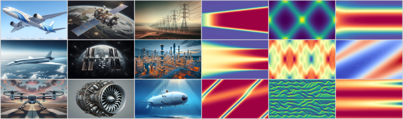
Figure 1: Environments included in this work, motivated by industrial control applications

1 Introduction

The intersection of machine learning (ML), reinforcement learning (RL), and control theory has garnered significant attention in recent years, giving rise to the learning for dynamics & control (L4DC) research community (Recht, 2019; Vamvoudakis et al., 2021; Brunke et al., 2022; Hu et al., 2023). L4DC has the naturally driven mission to unlock the power of learning-based methods for control and establish a rigorous theoretical foundation (L4DC, 2023). This mission could only be fulfilled with joint forces and close collaboration between theorists and practitioners from ML, control theory, and optimization.

On the one hand, theorists are keen to validate their algorithms and theories in real-world scenarios but encounter challenges with the complexity of OpenAI Gym/Gymnasium (Gym) environments (Brockman et al., 2016; Towers et al., 2023). Most Gym environments feature highly nonlinear dynamics, often involving contacts, and offer limited parameter customization options, making them ill-suited as testbeds for current theoretical studies. Meanwhile, simple control textbook examples lack the complexity required for cutting-edge ML/RL research that prioritizes efficiency and scalability. On the other hand, practitioners seek to evaluate their algorithms in realistic settings to validate their approaches and fuel theoretical developments.

To address these diverse requirements, we introduce controlgym, a lightweight and versatile Python library designed to support theorists and practitioners, offering a spectrum of environments that span from linear systems to chaotic, infinite-dimensional systems governed by partial differential equations (PDEs). Specifically, controlgym features thirty-six safety-critical linear industrial control environments, encompassing sectors like aerospace, cyber-physical systems, ground and underwater vehicles, and power systems. Additionally, controlgym includes ten infinite-dimensional PDE control environments relevant to fields such as fluid dynamics (Brunton and Noack, 2015) and physics. All environments comply with Gym and support standard implementations of RL algorithms (Sutton et al., 2000; Kakade, 2002; Schulman et al., 2015, 2017; Mnih et al., 2016; Sutton and Barto, 2018), e.g., as seen in stable-baselines3 (Raffin et al., 2021).

Our primary contribution is the introduction of a diverse array of control environments characterized by continuous and unbounded action-observation spaces, designed for safety-critical and large-scale systems. These environments, detailed in Tables 1 and 2, enhance Gym’s collection and are highly customizable to support theoretical advancement in L4DC. For example, users can manipulate the open-loop dynamics of PDEs by adjusting physical parameters, with explicit formulas relating parameters and eigenvalues available in linear PDE environments (cf., Section 3.1). Additionally, our ten PDE environments uniquely allow the users to extend system dimensionality to infinity while preserving the intrinsic dynamics, a key aspect for assessing the scalability of RL algorithms. The PDE solvers implemented to power controlgym are innovative, employing state-of-the-art schemes with exponential spatial convergence and high-order temporal accuracy masked behind a user-friendly discrete-time state-space formulation. Specifically for linear PDE environments, we have developed novel state-space models to evolve the PDE dynamics.

Leveraging its strengths, controlgym is a testbed for exploring three essential aspects of applying RL to continuous control. First, it aims to probe whether RL algorithms can consistently converge in learning control policies. Second, it examines the stability and robustness of the policy and training process, motivated by real-world safety-critical applications. Lastly, it assesses the scalability of RL algorithms in high-dimensional and potentially infinite-dimensional systems. With controlgym, we bridge the theoretical development and practical applicability of L4DC by providing a research platform that supports the establishment of a rigorous foundation.

Related works. The COMP$l_{e}$ib project (Leibfritz, 2004; Leibfritz and Lipinski, 2004) pioneered in offering standard control tasks, as MATLAB files, for analyzing model-based control algorithms. In the era of ML and RL, Gym (Brockman et al., 2016; Towers et al., 2023) has become the standard platform for developing and benchmarking RL algorithms for continuous control, offering a variety of environments such as cart pole, inverted pendulum, and robotic tasks powered by Mujoco (Todorov et al., 2012). Numerous follow-up projects that implement RL algorithms on Gym environments include rllab/garage (Duan et al., 2016), RLlib (Liang et al., 2018), dm$\_$control (Tunyasuvunakool et al., 2020), deluca (Gradu et al., 2020), stable-baselines3 (Raffin et al., 2021), safe-control-gym (Brunke et al., 2022), realworldrl-suite (Dulac-Arnold et al., 2020), tianshou (Weng et al., 2022), and TorchRL (Bou et al., 2023). Very recently, HydroGym (Callaham et al., 2023) provided fluid dynamics environments for testing RL algorithms for flow control.

Complying with Gym’s framework, we offer a spectrum of control environments designed to support the foundational theoretical developments in RL for linear optimal control (Fazel et al., 2018; Bu et al., 2019a; Tu and Recht, 2019; Mohammadi et al., 2021; Yang et al., 2019; Dean et al., 2020; Malik et al., 2020; Furieri et al., 2020; Simchowitz and Foster, 2020; Simchowitz et al., 2020; Hambly et al., 2021; Chen and Hazan, 2021; Perdomo et al., 2021; Li et al., 2021; Zhao and You, 2021; Jansch-Porto et al., 2022; Ozaslan et al., 2022; Ju et al., 2022; Lale et al., 2022; Duan et al., 2022; Zhang and Başar, 2023; Tang et al., 2023; Tsiamis et al., 2022; Ziemann et al., 2022; Duan et al., 2023), linear robust control and dynamic games (Agarwal et al., 2019; Gravell et al., 2019; Bu et al., 2019b; Zhang et al., 2019, 2021a; Yang et al., 2020; Zhang et al., 2021c, 2020, b; Keivan et al., 2022; Guo and Hu, 2022; Cui et al., 2023), estimation and filtering (Umenberger et al., 2022; Zhang et al., 2023a, b, c), and PDE control (Pan et al., 2018; Bucci et al., 2019; Liu and Wang, 2021; Degrave et al., 2022; Zeng et al., 2022; Vignon et al., 2023; Mowlavi et al., 2023; Werner and Peitz, 2023; Peitz et al., 2023).

Notations. In the paper, we follow the list of notations in the following table.

Notation	Description
$s_{k}$, $a_{k}$	system state and control input/action at discrete time $k$, respectively
$w_{k}$, $v_{k}$	stochastic noise or deterministic uncertainty at discrete time $k$
$n_{s}$, $n_{a}$, $n_{y}$	dimensionalities of state, action, and observation, respectively
$\Omega$, $L$, $x$, $u$	physical domain, domain length, spatial coordinates, and spatial field of PDE, respectively
$\Phi_{i}(x)$	time-invariant forcing support function for the $i^{th}$ control input $a_{i}$
$\Delta t,dt$	sampling time and numerical integration time step, respectively
$K$	total number of discrete time steps
$W$	discrete Fourier transform (DFT) matrix
$I$, $0$	Identity and zero matrices of appropriate dimensions, respectively
$c$	velocity in the convection-diffusion-reaction (CDR) and wave equations
$\nu$	diffusivity constant in CDR, Burgers’, Fisher, Allen-Cahn, and Cahn-Hilliard equations
$r$	reaction constant in CDR and Fisher equations
$\hbar,m$	Planck constant and particle mass, respectively, in the Schrödinger equation
$V$	potential constant in Schrödinger and Allen-Cahn equations
$\Gamma$	surface tension constant in the Cahn-Hilliard equation
$\psi$	local change rate of $u(x,t)$ in the wave equation
$\xi$, $\eta$	real and imaginary parts of $u(x,t)$ in the Schrödinger equation, respectively

2 Control Environments

2.1 Linear Control Environments

Table 1: List of the linear control environments in controlgym

ID	$n_{s}$	$n_{a}$	$n_{y}$	Task	ID	$n_{s}$	$n_{a}$	$n_{y}$	Task
ac1	5	3	3	aircraft	cm5	480	1	2	cable-mass model
ac2	5	3	3	aircraft	dis1	8	4	4	decentralized system
ac3	4	1	2	aircraft	dis2	4	2	2	decentralized system
ac4	9	1	2	aircraft	dlr	40	2	2	space structure
ac5	9	1	5	aircraft	he1	4	2	1	helicopter
ac6	10	4	5	aircraft	he2	8	4	6	helicopter
ac7	55	2	2	aircraft	he3	8	4	6	helicopter
ac8	4	3	4	aircraft	he4	8	4	2	helicopter
ac9	40	3	4	aircraft	he5	20	4	6	helicopter
ac10	10	2	2	aircraft	he6	20	4	6	helicopter
bdt1	11	3	3	distillation tower	iss	270	3	3	International Space Station
bdt2	82	4	4	distillation tower	je1	30	3	5	jet engine
cbm	348	1	1	clamped beam model	je2	24	3	6	jet engine
cdp	120	2	2	CD player	lah	48	1	1	L.A. University Hospital
cm1	20	1	2	cable-mass model	pas	5	1	3	piezoelectric bimorph actuator
cm2	60	1	2	cable-mass model	psm	7	2	3	power system
cm3	120	1	2	cable-mass model	rea	8	1	1	chemical reactor
cm4	240	1	2	cable-mass model	umv	8	2	2	underwater vehicle

We incorporate $36$ linear control environments from various industries, as detailed in Table 1. We select and organize these continuous-time linear systems from the pioneering COMP$l_{e}$ib project (Leibfritz, 2004; Leibfritz and Lipinski, 2004), and provide them as MATLAB-style .mat files in controlgym. These environments span control applications ranging from aircraft, helicopters, jet engines, reactor models, decentralized cyber-physical systems, binary distillation towers, ground and underwater autonomous vehicles, power systems, compact disk (CD) players, and large space structures. Additionally, the scope of our environments extends to control problems within projects such as the International Space Station and the Los Angeles Hospital.

With the user-selected sampling time $\Delta t$, we assume the control input is constant over each $\Delta t$ and generate the discrete-time system dynamics as

$$s_{k+1} =As_{k}+B_{1}w_{k}+B_{2}a_{k},$$

$$z_{k} =C_{1}s_{k}+D_{11}w_{k}+D_{12}a_{k},$$

$$y_{k} =Cs_{k}+D_{21}w_{k},$$

where $s_{k}\in\mathbb{R}^{n_{s}}$ is the state, $a_{k}$ is the control/action input, $w_{k}$ is the disturbance input that could be either stochastic or adversarial, $z_{k}\in\mathbb{R}^{n_{z}}$ is the output, $y_{k}\in\mathbb{R}^{n_{y}}$ is the observation, and $A$, $B_{1}$, $B_{2}$, $C_{1}$, $C$, $D_{11}$, $D_{12}$, $D_{21}$ are the discretized system matrices with appropriate dimensions. These linear control environments are directly applicable to support theoretical research of RL for the fundamental linear control, games, and estimation tasks (cf., Section 1).

Linear control objectives. For each linear control task in Table 1, we define a regulation task whose primary objective is to steer the system’s dynamics toward the zero vector. The reward function (to be maximized) is formulated as the negative sum of the linear-quadratic (LQ) stage cost

$$\mathcal{J}(a_{k})=-\mathbb{E}\Big{\{}\sum_{k=0}^{K-1}(s_{k}^{\top}Qs_{k}+a_{k}^{\top}Ra_{k}+2s_{k}^{\top}Sa_{k})\Big{\}},$$

where $Q=C_{1}^{\top}C_{1}$, $R=D_{12}^{\top}D_{12}$, and $S=C_{1}^{\top}D_{12}$ aim to balance regulation performance and control efforts, and $K$ is the total number of discrete time steps.

2.2 PDE Control Environments

Table 2: List of PDE control environments in controlgym

ID	$n_{s}$	$n_{a}$	$n_{y}$	Linearity
convection_diffusion_reaction	$(50,+\infty)$	$(1,+\infty)$	$(1,+\infty)$	Linear
wave	$(100,+\infty)$	$(1,+\infty)$	$(1,+\infty)$	Linear
schrodinger	$(100,+\infty)$	$(1,+\infty)$	$(1,+\infty)$	Linear
burgers	$(50,+\infty)$	$(1,+\infty)$	$(1,+\infty)$	Nonlinear
kuramoto_sivashinsky	$(200,+\infty)$	$(1,+\infty)$	$(1,+\infty)$	Nonlinear
fisher	$(50,+\infty)$	$(1,+\infty)$	$(1,+\infty)$	Nonlinear
allen_cahn	$(50,+\infty)$	$(1,+\infty)$	$(1,+\infty)$	Nonlinear
korteweg_de_vries	$(200,+\infty)$	$(1,+\infty)$	$(1,+\infty)$	Nonlinear
cahn_hilliard	$(50,+\infty)$	$(1,+\infty)$	$(1,+\infty)$	Nonlinear
ginzburg_landau	$(50,+\infty)$	$(1,+\infty)$	$(1,+\infty)$	Nonlinear

In this section, we describe one-dimensional PDE control environments with periodic boundary conditions and spatially distributed control inputs. We first define a spatial domain $\Omega=[0,L]\subset\mathbb{R}$ and a continuous field $u(x,t):\Omega\times\mathbb{R}^{+}\rightarrow\mathbb{R}$, where $x$ and $t$ represent spatial and temporal coordinates, respectively, and $L$ is the length of the domain. Each PDE control task listed in Table 2 then takes the general continuous form

$$\frac{\partial u}{\partial t}-\mathcal{F}\left(\frac{\partial u}{\partial x},\frac{\partial^{2}u}{\partial x^{2}},\dots\right)=a(x,t),$$ (2.1)

where $\mathcal{F}$ is a linear or nonlinear differential operator (see Sections 2.2.1-2.2.10 for specific definitions for each PDE) that contains spatial derivatives of various orders and depends on various physical constants, and $a$ is a distributed control force defined as

$$a(x,t)=\sum_{j=0}^{n_{a}-1}\Phi_{j}(x)a_{j}(t).$$ (2.2)

The control force consists of $n_{a}$ scalar control inputs $a_{j}(t)$, each acting over a specific subset of $\Omega$ defined by its corresponding forcing support function $\Phi_{j}(x)$, as illustrated in Figure 2. Such a control force can be used to model the addition of energy to the system or other external influences that affect the PDE dynamics. We use periodic boundary conditions in all of our PDE control tasks, meaning that $u$ and all its spatial derivatives are equal at both ends of the domain $\Omega$.

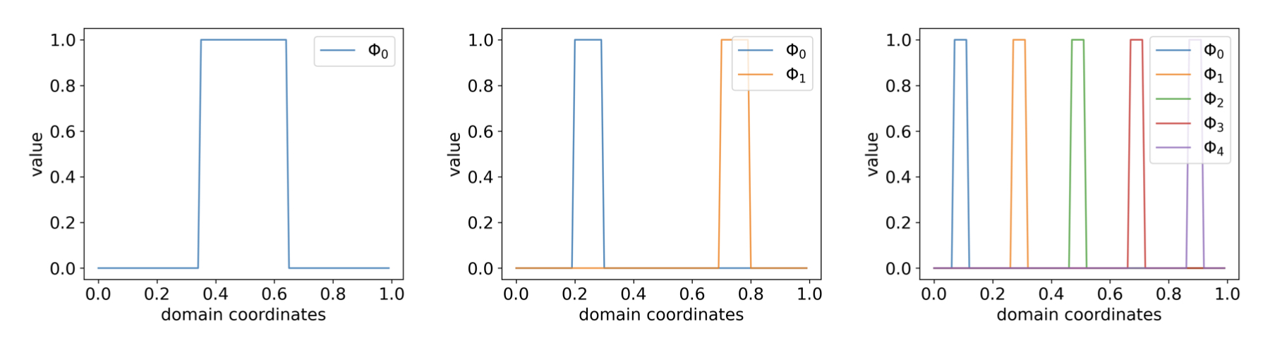
Figure 2: Illustration of how distributed control inputs influence the dynamics of a PDE through forcing support functions $\Phi_{j}$, taking $\Omega=[0,1]$ as an example. Left: The forcing support function corresponding to a single control input is depicted, with its width, a tunable parameter, set to $0.3$. This represents a control input that uniformly affects state components spanning the middle $30\%$ of the physical domain. Middle: The forcing support functions corresponding to two control inputs are shown. They are spaced equidistantly from one another, and each has a width of $0.1$ so that each control input uniformly affects state components spanning $10\%$ of the physical domain. Right: The forcing support functions corresponding to five control inputs are shown, each with a width of $0.05$ uniformly affecting state components spanning $5\%$ of the physical domain.

Discretization of space and time. To solve the PDEs listed in Table 2, we first need to discretize space and time in the continuous form (2.1). For a state dimension $n_{s}$ that is even and a sampling time $\Delta t\in\mathbb{R}^{+}$, both selected by the user, we define a state vector $s_{k}\in\mathbb{R}^{n_{s}}$ that contains the values of $u$ at $n_{s}$ equally-spaced points in $\Omega$ and at discrete time $k\in\mathbb{N}$ corresponding to the simulation time $t=k\,\Delta t$. The total simulation time is $K\,\Delta t$, where $K\in\mathbb{N}$ is an input parameter specifying the total number of discrete-time steps. We also assume that the scalar control inputs $a_{i}(t)$ are piecewise constant over each discrete-time step of duration $\Delta t$ so that they can be concatenated into a discrete-time vector $a_{k}\in\mathbb{R}^{n_{a}}$ for all $k\in\{0,\cdots,K-1\}$.

Numerical solver for nonlinear PDEs. After discretizing space and time, the dynamics of the nonlinear PDEs can be approximated by a discrete-time finite-dimensional nonlinear system

$$s_{k+1}=f(s_{k},a_{k};w_{k}),$$ (2.3)

where $f:\mathbb{R}^{n_{s}}\times\mathbb{R}^{n_{a}}\to\mathbb{R}^{n_{s}}$ is a time-invariant mapping contingent on the physical parameters of each specific PDE and forcing support functions $\Phi_{i}$, and $w_{k}$ is an optional stochastic process noise. To compute the mapping $f$, we numerically approximate the space and time derivatives in (2.1) using, respectively, a pseudo-spectral method (Trefethen, 1996) and a fourth-order exponential time differencing Runge-Kutta (ETDRK4) scheme (Cox and Matthews, 2002; Kassam and Trefethen, 2005). We then integrate numerically the dynamics over one discrete-time step of duration $\Delta t$ using an internal integration time step $dt$. The mapping $f$ is therefore not obtained explicitly; rather, its action is evaluated through a numerical integration loop. The sampling time $\Delta t$ may be selected as large as desired, but it should be an integer multiple of the integration time step $dt$.

In general, one should choose $n_{s}$ to be sufficiently large and $dt$ to be sufficiently small to ensure the accuracy of the discretized system (2.3). Due to the exponential convergence rate of the pseudo-spectral method as well as the high convergence rate of the ETDRK4 scheme, $n_{s}$ larger than about 50 is sufficient in most cases, except the Korteweg de Vries and Kuramoto-Sivashinsky PDEs that require $n_{s}$ larger than about 200 for accurate solutions. For all PDEs, the presence of small-scale (i.e., high wavenumber) spatial features in the initial condition may necessitate higher values of $n_{s}$.

Explicit state-space model for linear PDEs. After space and time discretization, the linear PDEs listed in Table 2 can be approximated by a discrete-time linear state-space model of the form

$$s_{k+1}=As_{k}+B_{2}a_{k}+w_{k},$$ (2.4)

where $A\in\mathbb{R}^{n_{s}\times n_{s}}$ is a time-invariant transition matrix contingent on the physical parameters of each specific PDE, $B_{2}\in\mathbb{R}^{n_{s}\times n_{a}}$ is a time-invariant control matrix, and $w_{k}\sim\mathcal{N}(0,\Sigma_{w})$ is an optional process noise. The $A$ matrix in (2.4) is constructed from a spectral approximation of the space derivatives in (2.1) combined with an analytical temporal integration of the continuous-time linear dynamics over one discrete-time step of duration $\Delta t$ (see Sections 2.2.1-2.2.3 for detailed treatments of each case). Contrary to the case of nonlinear PDEs where evaluating the mapping $f$ in (2.3) requires an internal numerical integration loop, the availability of matrix $A$ in explicit form for linear PDEs allows for the direct application of model-based linear controllers.

Similar to nonlinear PDEs, due to the numerical approximation of the spatial derivatives, one should choose $n_{s}$ to be sufficiently large to ensure the accuracy of the state-space model (2.4), with $n_{s}$ greater than about 50 sufficient in most cases. Due to the analytical temporal integration of the dynamics, there is no internal integration time step $dt$ to select. As in the nonlinear case, the sampling time $\Delta t$ may be chosen as large as desired.

Since the state-space model (2.4) is derived from a PDE, the eigenvalues and eigenvectors of the $A$ matrix can be analyzed explicitly. This method allows for a clearer understanding of the impact of the PDE’s physical parameters on the system dynamics, such as open-loop stability. By adjusting these parameters, users can tailor the system dynamics to better assess their algorithms. We demonstrate this process with the convection-diffusion-reaction equation in Section 3.1, illustrating the relationships between its physical parameters and open-loop system dynamics.

Observation process. For all PDEs listed in Table 2, we place $n_{y}$ sensors uniformly throughout the domain $\Omega$, where each sensor measures the unscaled value of the state at its location, perturbed by additive zero-mean Gaussian white noise. That is, the observation $y_{k}$ at time $k$ is computed by $y_{k}=Cs_{k}+v_{k}$, where $C\in\mathbb{R}^{n_{y}\times n_{s}}$ is structured with a single $1$ per row and zeros elsewhere, and $v_{k}\sim\mathcal{N}(0,\Sigma_{v})$. Both $n_{y}$ and $\Sigma_{v}$ are user-configurable parameters.

PDE control objectives. For all PDEs listed in Table 2, we define a control task whose primary objective is to steer the system’s dynamics toward a user-defined target state $s_{ref}\in\mathbb{R}^{n_{s}}$. The reward function is formulated as the negative sum of the LQ stage cost

$$\mathcal{J}(a_{k})=-\mathbb{E}\left\{\sum_{k=0}^{K-1}\Big{[}(s_{k}-s_{ref})^{\top}Q(s_{k}-s_{ref})+a_{k}^{\top}Ra_{k}\Big{]}\right\},$$

where $Q$ and $R$ are positive-definite weighting matrices that balance tracking performance and control effort. When the target state is the zero vector, the tracking problem reduces to the LQ regulation problem.

2.2.1 Convection-Diffusion-Reaction Equation

The convection-diffusion-reaction (CDR) equation models the transfer of particles, energy, or other physical quantities within a system due to convection, diffusion, and reaction processes. The temporal dynamics of the continuous concentration function $u(x,t)$ in one spatial dimension is given by

$$\frac{\partial u}{\partial t}+c\,\frac{\partial u}{\partial x}-\nu\,\frac{\partial^{2}u}{\partial x^{2}}-r\,u=a(x,t),$$ (2.5)

where $c$ is the convection velocity, $\nu>0$ is the diffusivity constant, $r$ is the reaction constant, and $a(x,t)$ is a source term defined in (2.2) that models the addition of energy to the system or other external influences that affect the PDE dynamics. The scalar physical parameters of the CDR equation characterize the strength of convection, diffusion, and reaction processes. When $c=r=0$, the CDR equation (2.5) reduces to the heat equation. The CDR equation with $r=0$ has been used to validate the global convergence of RL algorithms in Kalman filtering (Zhang et al., 2023b). We visualize the uncontrolled solution of the CDR equation for a specific choice of parameters and initial condition in Figure 3.

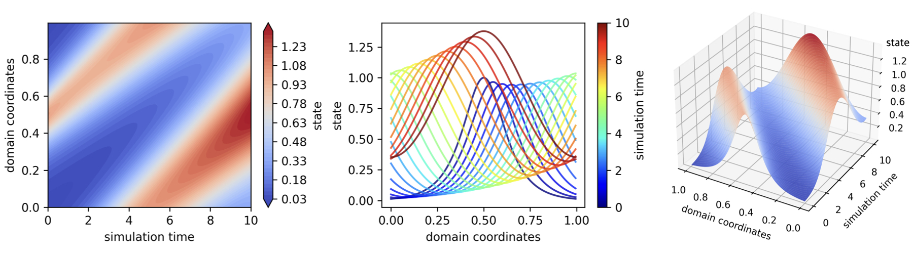
Figure 3: The uncontrolled solution to the CDR equation in a domain of length $L=1$ with parameters, $c=0.01$, $\nu=0.002$, and $r=0.1$. The initial condition is $u(x,t=0)=\mathrm{sech}(10x-5)$. Left: Contour plot that shows the value of the state variable over the total simulation time ($x$-axis) and across the spatial domain ($y$-axis). Middle: Lines representing the state variable at fixed times. The $x$- and $y$-axes represent spatial coordinates and values of the state variable, respectively. The color of the lines corresponds to different time stamps within the total simulation time. Right: 3D surface plot showing the value of the state variable ($z$-axis) over time ($y$-axis) and across the spatial domain ($x$-axis).

After discretizing space and time, the CDR equation can be approximated by the linear state-space model (2.4) with

$$A=\frac{1}{n_{s}}W^{\dagger}{\rm diag}(e^{(-ick_{x}-\nu k_{x}^{2}+r)\Delta t})W,\quad B_{2}=\left[\begin{array}[]{c|c|c|c}\Phi_{0}&\Phi_{1}&\cdots&\Phi_{n_{a}-1}\end{array}\right]\in\mathbb{R}^{n_{s}\times n_{a}}$$ (2.7)

where $i$ is the imaginary unit, $k_{x}=\frac{2\pi}{L}[0,\dots,\frac{n_{s}}{2}-1,0,-\frac{n_{s}}{2}+1,\dots,-1]\in\mathbb{R}^{n_{s}}$ is the vector of spatial wavenumbers, $\Phi_{j}\in\mathbb{R}^{n_{s}}$ are the forcing support functions evaluated at $n_{s}$ equally-spaced points in $\Omega$, and $W\in\mathbb{R}^{n_{s}\times n_{s}}$ is the discrete Fourier transform (DFT) matrix with entries defined by (Rao and Yip, 2018)

$$\forall p,q,\quad W_{pq}=e^{-\frac{2\pi i(p-1)(q-1)}{n_{s}}}.$$ (2.8)

The scaled conjugate transpose of $W$, denoted by $W^{\dagger}/n_{s}$, is the inverse DFT matrix. In Section 3.1, we present the analytical eigenvalues and eigenvectors of the $A$ matrix in (2.7), derived as functions of the physical parameters of the CDR equation.

2.2.2 Wave Equation

The wave equation is a fundamental linear PDE in physics and engineering, describing the propagation of various types of waves through a homogeneous medium. The temporal dynamics of the perturbed scalar quantity $u(x,t)$ propagating as a wave through one-dimensional space is given by

$$\frac{\partial^{2}u}{\partial t^{2}}-c^{2}\,\frac{\partial^{2}u}{\partial x^{2}}=a(x,t),$$ (2.9)

where $c$ is a constant representing the wave’s speed in the medium, and $a(x,t)$ is a source term defined in (2.2) that models the effect of a force or other external influences acting on the system. We visualize the uncontrolled solution of the wave equation for a specific choice of parameters and initial condition in Figure 4.

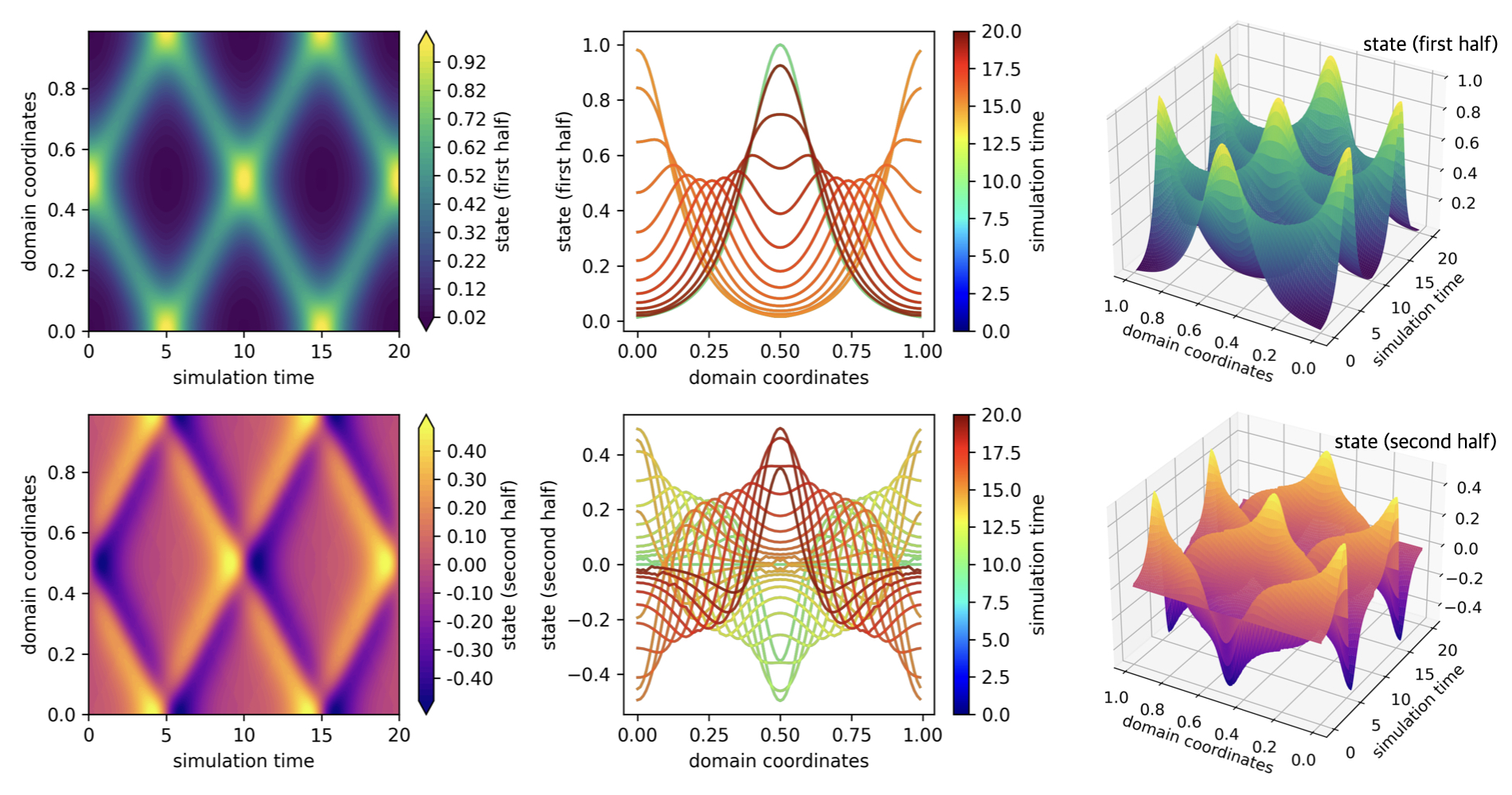
Figure 4: The uncontrolled solution to the wave equation in a domain of length $L=1$ with parameter $c=0.1$. The initial conditions are $u(x,t=0)=\mathrm{sech}(10x-5)$ and $\psi(x,t=0)=0$. The figure convention is consistent with that of Figure 3.

We solve the wave equation by first transforming (2.9) into a coupled system of two PDEs with first-order time derivatives. Specifically, we introduce a second continuous field $\psi(x,t):\Omega\times\mathbb{R}^{+}\rightarrow\mathbb{R}$ representing the rate at which the scalar quantity $u(x,t)$ is changing locally. Then, we can write (2.9) in the equivalent form

$$\frac{\partial u}{\partial t}-\psi =0,$$ (2.10a)

$$\frac{\partial\psi}{\partial t}-c^{2}\,\frac{\partial^{2}u}{\partial x^{2}} =a(x,t).$$ (2.10b)

We next discretize space and time by introducing a state vector $s_{k}$ that concatenates the values of both $u$ and $\psi$, each sampled at $n_{s}^{\prime}=n_{s}/2$ equally-spaced points in $\Omega$ so that $s_{k}$ contains $n_{s}$ components. The wave equation in the form (2.10) can then be approximated by the state-space model (2.4) with

$$A =\frac{1}{n_{s}^{\prime}}\cdot\left[\begin{array}[]{c|c}W&0_{n_{s}^{\prime}\times n_{s}^{\prime}}\\ \hline\cr 0_{n_{s}^{\prime}\times n_{s}^{\prime}}&W\end{array}\right]^{\dagger}\exp\left(\left[\begin{array}[]{c|c}0_{n_{s}^{\prime}\times n_{s}^{\prime}}&I_{n_{s}^{\prime}\times n_{s}^{\prime}}\\ \hline\cr\Lambda&0_{n_{s}^{\prime}\times n_{s}^{\prime}}\end{array}\right]\Delta t\right)\left[\begin{array}[]{c|c}W&0_{n_{s}^{\prime}\times n_{s}^{\prime}}\\ \hline\cr 0_{n_{s}^{\prime}\times n_{s}^{\prime}}&W\end{array}\right]$$ (2.17)

$$B_{2} =\left[\begin{array}[]{c|c|c|c}0_{n_{s}^{\prime}}&0_{n_{s}^{\prime}}&\cdots&0_{n_{s}^{\prime}}\\ \hline\cr\Phi_{0}^{\prime}&\Phi_{1}^{\prime}&\cdots&\Phi_{n_{a}-1}^{\prime}\end{array}\right]\in\mathbb{R}^{n_{s}\times n_{a}},$$ (2.20)

where $\Lambda={\rm diag}(-c^{2}k_{x}^{2})\in\mathbb{R}^{n_{s}^{\prime}\times n_{s}^{\prime}}$ with $k_{x}=\frac{2\pi}{L}[0,\dots,\frac{n_{s}^{\prime}}{2}-1,0,-\frac{n_{s}^{\prime}}{2}+1,\dots,-1]\in\mathbb{R}^{n_{s}^{\prime}}$ the vector of spatial wavenumbers, $\Phi_{j}^{\prime}\in\mathbb{R}^{n_{s}^{\prime}}$ are the forcing support functions evaluated at $n_{s}^{\prime}$ equally-spaced points in $\Omega$, and $W\in\mathbb{R}^{n_{s}^{\prime}\times n_{s}^{\prime}}$ is the DFT matrix (2.8) but with $n_{s}$ replaced by $n_{s}^{\prime}$.

2.2.3 Schrödinger Equation

The Schrödinger equation is fundamental in quantum mechanics, describing how the quantum state of an isolated quantum-mechanical system, a complex-valued wave function, changes over time. For a single non-relativistic particle in a constant potential, the Schrödinger equation for the wave function $u(x,t)$ is given by

$$i\hbar\frac{\partial u}{\partial t}+\frac{\hbar^{2}}{2m}\frac{\partial^{2}u}{\partial x^{2}}-V\,u=\hbar\,a(x,t),$$ (2.21)

where $i$ is the imaginary unit, $\hbar$ is the Planck constant, $V$ is the real potential constant, and $a(x,t)$ is a real-valued source term defined in (2.2) that models a force acting on the system or other external influences that affect the PDE dynamics. We visualize the uncontrolled solution of the Schrödinger equation for a specific choice of parameters and initial condition in Figure 5.

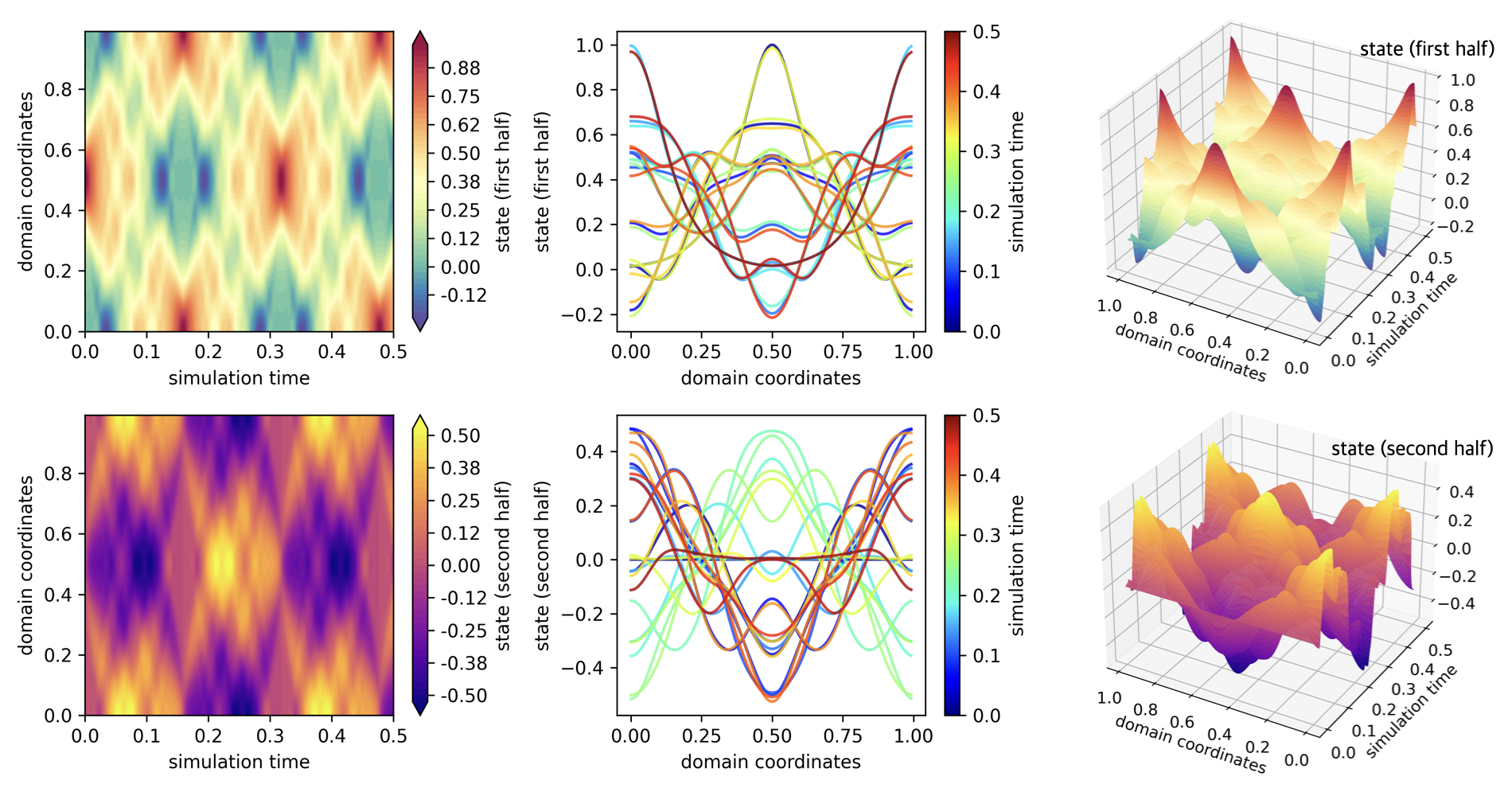
Figure 5: The uncontrolled solution to the Schrödinger equation in a domain of length $L=1$ with parameters $\hbar=1.0$, $m=1.0$, and $V=0.0$. The initial conditions are $\xi(x,t=0)=\mathrm{sech}(10x-5)$ and $\eta(x,t=0)=0$. The figure convention is consistent with that of Figure 3.

We solve the Schrödinger equation by first transforming (2.21) into a coupled system of two PDEs with first-order time derivatives, similar to the approach adopted for the wave equation. Specifically, we introduce two continuous fields $\xi(x,t):\Omega\times\mathbb{R}^{+}\rightarrow\mathbb{R}$ and $\eta(x,t):\Omega\times\mathbb{R}^{+}\rightarrow\mathbb{R}$ that represent the real and imaginary parts of the complex-valued scalar quantity $u(x,t)$, respectively. Then, we rewrite (2.9) in the equivalent form

$$\frac{\partial\xi}{\partial t}+\frac{\hbar}{2m}\frac{\partial^{2}\eta}{\partial x^{2}}-\frac{V}{\hbar}\eta =0,$$ (2.22a)

$$\frac{\partial\eta}{\partial t}-\frac{\hbar}{2m}\frac{\partial^{2}\xi}{\partial x^{2}}+\frac{V}{\hbar}\xi =a(x,t),$$ (2.22b)

We now discretize space and time by introducing a state vector $s_{k}$ that concatenates the values of both $\xi$ and $\eta$, each sampled at $n_{s}^{\prime}=n_{s}/2$ equally-spaced points in $\Omega$ so that $s_{k}$ contains $n_{s}$ components. The Schrödinger equation in the form (2.10) can then be approximated by the state-space model (2.4) with

$$A =\frac{1}{n_{s}^{\prime}}\left[\begin{array}[]{c|c}W&0_{n_{s}^{\prime}\times n_{s}^{\prime}}\\ \hline\cr 0_{n_{s}^{\prime}\times n_{s}^{\prime}}&W\end{array}\right]^{\dagger}\exp\left(\left[\begin{array}[]{c|c}0_{n_{s}^{\prime}\times n_{s}^{\prime}}&\Lambda\\ \hline\cr-\Lambda&0_{n_{s}^{\prime}\times n_{s}^{\prime}}\end{array}\right]\Delta t\right)\left[\begin{array}[]{c|c}W&0_{n_{s}^{\prime}\times n_{s}^{\prime}}\\ \hline\cr 0_{n_{s}^{\prime}\times n_{s}^{\prime}}&W\end{array}\right],$$ (2.29)

$$B_{2} =\left[\begin{array}[]{c|c|c|c}0_{n_{s}^{\prime}}&0_{n_{s}^{\prime}}&\cdots&0_{n_{s}^{\prime}}\\ \hline\cr\Phi_{0}^{\prime}&\Phi_{1}^{\prime}&\cdots&\Phi_{n_{a}-1}^{\prime}\end{array}\right]\in\mathbb{R}^{n_{s}\times n_{a}},$$ (2.32)

where $\Lambda={\rm diag}(\hbar/(2m)k_{x}^{2}+V/\hbar)\in\mathbb{R}^{n_{s}^{\prime}\times n_{s}^{\prime}}$ with $k_{x}=\frac{2\pi}{L}[0,\dots,\frac{n_{s}^{\prime}}{2}-1,0,-\frac{n_{s}^{\prime}}{2}+1,\dots,-1]\in\mathbb{R}^{n_{s}^{\prime}}$ the vector of spatial wavenumbers, $\Phi_{j}^{\prime}\in\mathbb{R}^{n_{s}^{\prime}}$ are the forcing support functions evaluated at $n_{s}^{\prime}$ equally-spaced points in $\Omega$, and $W\in\mathbb{R}^{n_{s}^{\prime}\times n_{s}^{\prime}}$ is the DFT matrix defined in (2.8) but with $n_{s}$ therein replaced by $n_{s}^{\prime}$.

2.2.4 Burgers’ Equation

Burgers’ equation is a simplified version of nonlinear PDEs arising in fluid dynamics and captures key features of water waves and gas dynamics such as shock formation. The temporal dynamics of the velocity $u(x,t)$ is

$$\frac{\partial u}{\partial t}+u\frac{\partial u}{\partial x}-\nu\frac{\partial^{2}u}{\partial x^{2}}=a(x,t),$$ (2.33)

where $\nu>0$ is the diffusivity (or viscosity) parameter and $a(x,t)$ is a source term defined in (2.2) that models a force acting on the system or other external influences that affect the PDE dynamics. At the inviscid limit of $\nu=0$, Burgers’ equation predicts discontinuous shocks; at low $\nu$ values, Burgers’ equation exhibits shock-like behavior but remains smooth; and with high values of $\nu$, Burgers’ equation mirrors the dissipative nature of the heat equation. The behavior of the uncontrolled solution for a specific choice of parameters and initial condition is shown in Figure 6.

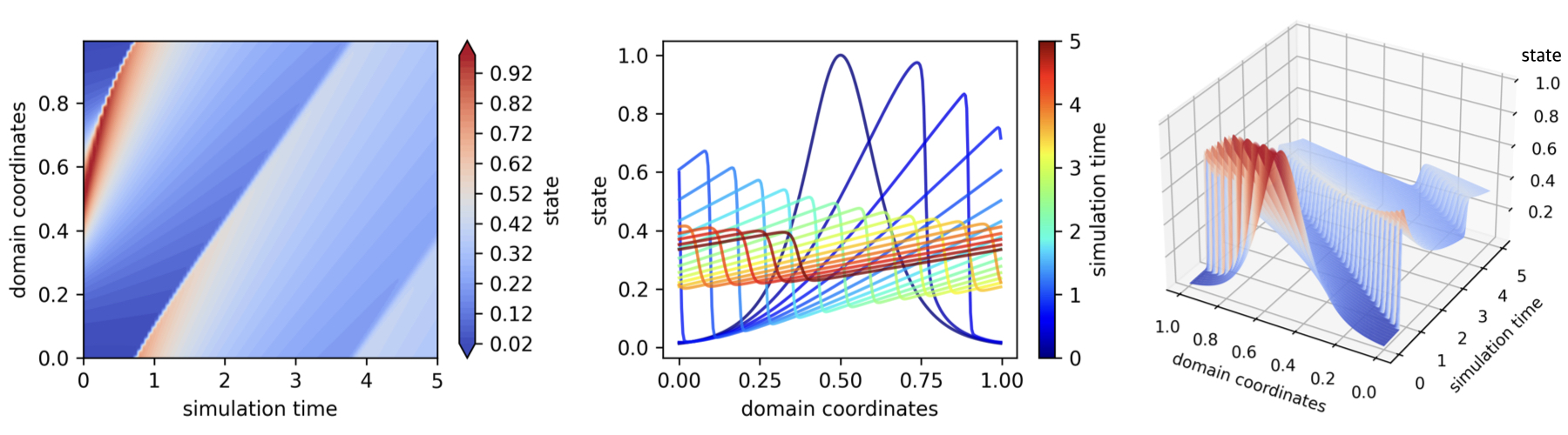
Figure 6: The uncontrolled solution to Burgers’ equation in a domain of length $L=1$ with parameter $\nu=0.001$. The initial condition is $u(x,t=0)=\mathrm{sech}(10x-5)$. The figure convention is consistent with that of Figure 3.

2.2.5 Kuramoto-Sivashinsky Equation

The Kuramoto-Sivashinsky (KS) equation is a nonlinear PDE applied to studying pattern formation and instability in fluid dynamics, combustion, and plasma physics. The temporal dynamics of $u(x,t)$ in one spatial dimension is provided by

$$\frac{\partial u}{\partial t}+u\frac{\partial u}{\partial x}+\frac{\partial^{2}u}{\partial x^{2}}+\frac{\partial^{4}u}{\partial x^{4}}=a(x,t),$$ (2.34)

where $a(x,t)$ is a source term defined in (2.2) that models a force acting on the system or other external influences that affect the dynamics. The nonlinear convection term, the second-order diffusion term, and the fourth-order dispersion term interact to produce complex spatial patterns and temporal chaos when the domain length $L$ is large enough (Cvitanović et al., 2010). Figure 7 displays the behavior of the uncontrolled solution of the KS equation for a specific initial condition and $L=32\pi$, well into the chaotic regime. Due to the chaotic nature of the dynamics, the specific choice of initial condition has negligible influence on the qualitative properties of the solution.

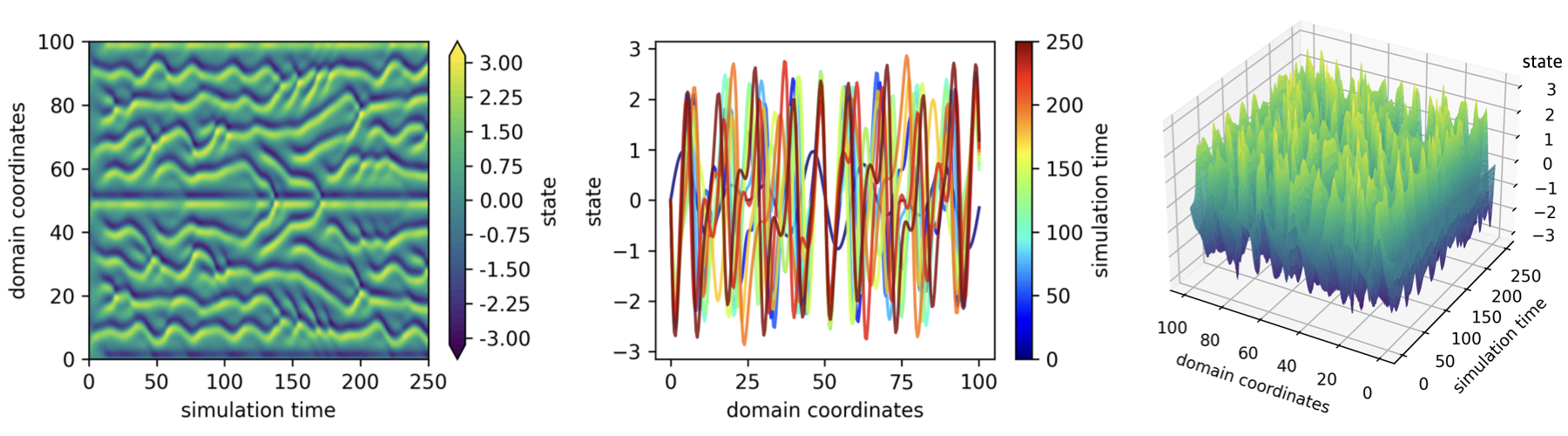
Figure 7: The uncontrolled solution to the KS equation in a domain of length $L=32\pi$. The initial condition is $u(x,t=0)=\frac{1}{16}x\,\sin(\frac{3}{8}x)$ . The figure convention is consistent with that of Figure 3.

2.2.6 Fisher Equation

The Fisher equation is a nonlinear PDE employed in biology, ecology, and epidemiology to model gene propagation, invasions, and population dynamics. The temporal dynamics of $u(x,t)$ in one spatial dimension is described by

$$\frac{\partial u}{\partial t}-\nu\frac{\partial^{2}u}{\partial x^{2}}-r\cdot u(1-u)=a(x,t),$$ (2.35)

where $\nu>0$ is the diffusivity constant, $r$ is the reaction constant, and $a(x,t)$ is a source term defined in (2.2) that models external influences affecting the PDE dynamics. The term $r\cdot u(1-u)$ captures population expansion limited by carrying capacity, with $r$ as the intrinsic growth rate. The uncontrolled solution of the Fisher equation for a specific choice of parameters and initial condition is depicted in Figure 8.

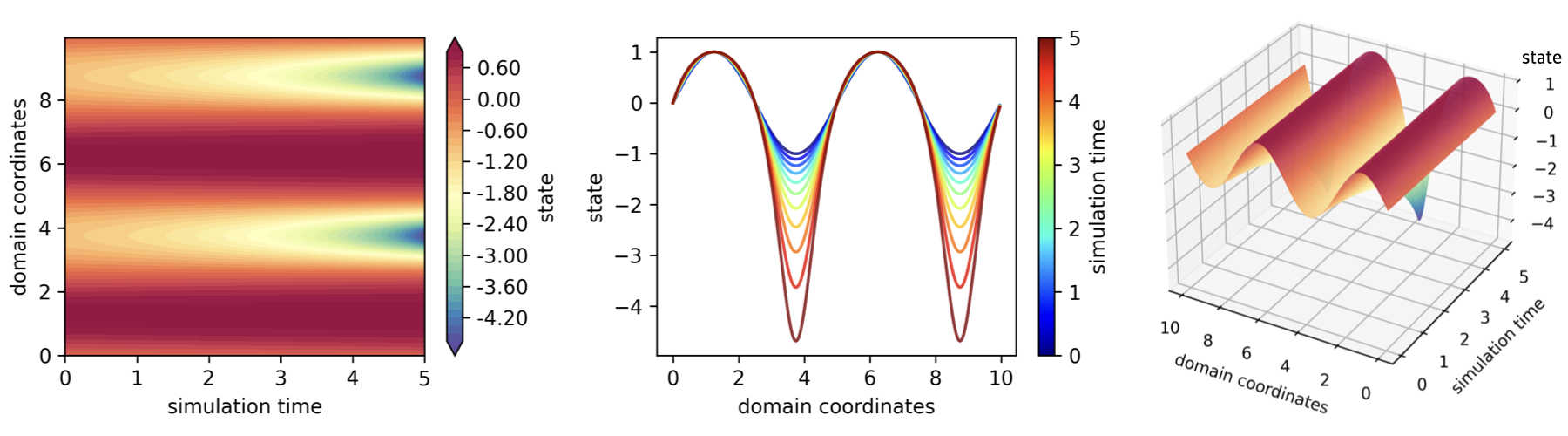
Figure 8: The uncontrolled solution to the Fisher equation in a domain of length $L=10$ with parameters $\nu=0.0001$ and $r=0.1$. The initial condition is $u(x,t=0)=\sin(\frac{2\pi x}{5})$. The figure convention is consistent with that of Figure 3.

2.2.7 Allen-Cahn Equation

The Allen-Cahn equation is a nonlinear PDE modeling phase separation in binary alloy systems in materials science. The temporal dynamics of $u(x,t)$ in one spatial dimension, with $u=\pm 1$ indicating the presence of one phase or the other, is given by

$$\frac{\partial u}{\partial t}-\nu^{2}\frac{\partial^{2}u}{\partial x^{2}}+V(u^{3}-u)=a(x,t),$$ (2.36)

where $\nu>0$ is the diffusivity constant, $V$ is the potential constant, and $a(x,t)$ is a source term defined in (2.2) that models external influences affecting the PDE dynamics. We visualize the uncontrolled solution of the Allen-Cahn equation for a specific choice of parameters and initial condition in Figure 9.

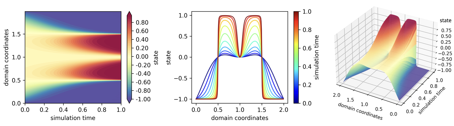
Figure 9: The uncontrolled solution to the Allen-Cahn equation in a domain of length $L=2$ with parameters $\nu=0.0001$ and $V=5.0$. The initial condition is $u(x,t=0)=(x-1)^{2}\cdot\cos(\pi(x-1))$. The figure convention is consistent with that of Figure 3.

2.2.8 Korteweg-de Vries Equation

The Korteweg-de Vries (KdV) equation is a nonlinear PDE pivotal in understanding nonlinear wave dynamics, modeling solitary wave propagation across shallow water surfaces, with applications extending to plasma physics, nonlinear optics, and quantum mechanics. The temporal dynamics of $u(x,t)$ with an additional source term $a(x,t)$ that models external influences is given by

$$\frac{\partial u}{\partial t}+\frac{\partial^{3}u}{\partial x^{3}}-6u\frac{\partial u}{\partial x}=a(x,t).$$ (2.37)

We visualize the uncontrolled solution of the KdV equation for a specific choice of parameters and an initial condition that leads to two solitons propagating at different speeds in Figure 10.

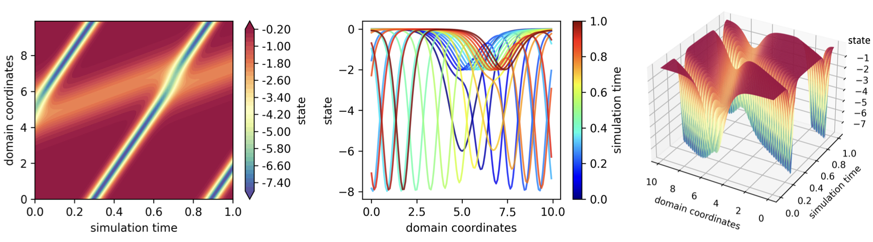
Figure 10: The uncontrolled solution to the KdV equation in a domain of length $L=10$. The initial condition is $u(x,t=0)=\frac{-12(3+\cosh(20-4x)+4\cosh(10-2x))}{(\cosh(15-3x)+3\cosh(5-x))^{2}}$. The figure convention is consistent with that of Figure 3.

2.2.9 Cahn-Hilliard Equation

The Cahn-Hilliard equation is a nonlinear PDE modeling phase separation in alloys and polymers in materials science. The temporal dynamics of $u(x,t)$ in one spatial dimension, with $u=\pm 1$ indicating the presence of one phase or the other, is described by

$$\frac{\partial u}{\partial t}-\nu\frac{\partial^{2}}{\partial x^{2}}(u^{3}-u-\Gamma\frac{\partial^{2}u}{\partial x^{2}})=a(x,t),$$ (2.38)

where $\nu>0$ is the diffusivity constant, $\Gamma$ is the constant surface tensor coefficient, and $a(x,t)$ is a source term defined in (2.2) that models external influences affecting the PDE dynamics. We visualize the uncontrolled solution of the Cahn-Hilliard equation for a specific choice of parameters and initial condition in Figure 11.

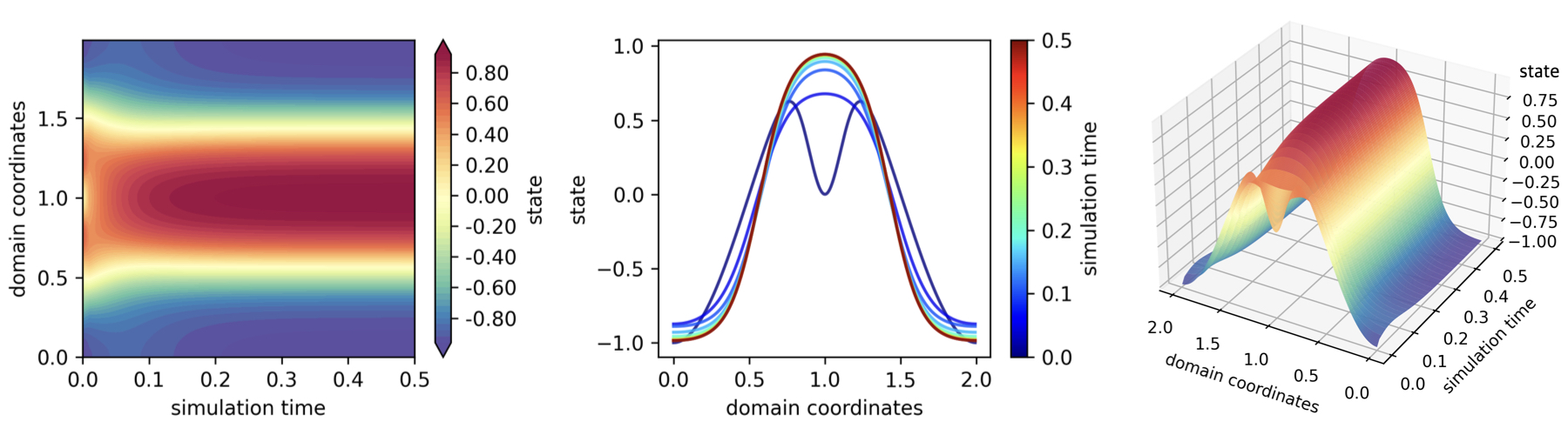
Figure 11: The uncontrolled solution to the Cahn-Hilliard equation in a domain of length $L=2$ with parameters $\nu=1.0$ and $\Gamma=0.02$. The initial condition is $u(x,t=0)=\cos(\pi(x-1))-\exp(-4(\pi(x-1))^{2})$. The figure convention is consistent with that of Figure 3.

2.2.10 Ginzburg-Landau Equation

The Ginzburg-Landau equation is a nonlinear PDE describing the evolution of disturbances near the onset of instability in various physical systems. The temporal dynamics of the amplitude $u(x,t)$ of a disturbance in one spatial dimension is governed by

$$\frac{\partial u}{\partial t}-u+|u|^{2}u-\frac{\partial^{2}u}{\partial x^{2}}=a(x,t),$$ (2.39)

where $a(x,t)$ is a source term defined in (2.2) that models external influences affecting the PDE dynamics. We visualize the uncontrolled solution of the Ginzburg-Landau equation for a specific choice of parameters and initial condition in Figure 12.

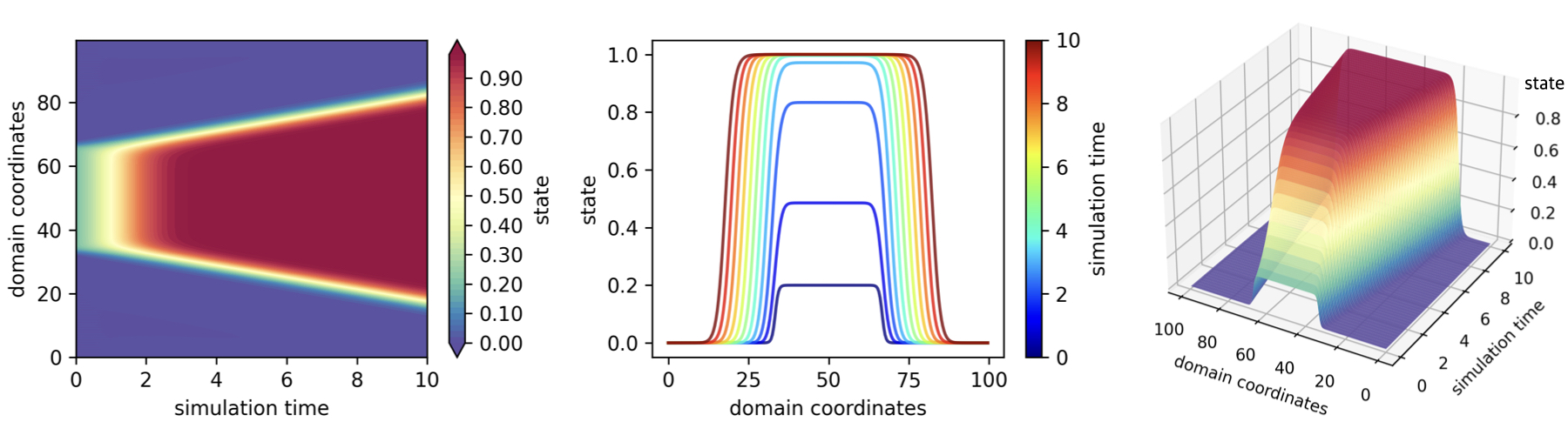
Figure 12: The uncontrolled solution to the Ginzburg-Landau equation in a domain of length $L=100$. The initial condition is $u(x,t=0)=\frac{1}{10}(\tanh(x-\frac{100}{3})-\tanh(x-\frac{200}{3}))$. The figure convention is consistent with that of Figure 3.

3 Examples of Using controlgym

This section provides several examples for using controlgym. In particular, we include a detailed analysis of how users can design the open-loop dynamics of linear PDEs by selecting physical parameters in Section 3.1. Sections 3.2 and 3.3 provide code examples of applying a model-based controller (as baseline) and an RL-based controller to a helicopter environment, respectively. Lastly, we demonstrate in Section 3.4 how to obtain the uncontrolled PDE trajectories displayed in Figures 3-12 using a code example.

3.1 Analysis of the Open-Loop Dynamics of Linear PDEs

Evaluating learning algorithms effectively involves designing and tuning the open-loop dynamics of control environments, for adjusting the control difficulties. Precisely, in linear PDE environments, the open-loop dynamics is entirely specified by the spectral properties of matrix $A$ in (2.4). Using the CDR equation from Section 2.2.1 as a case study, we demonstrate the analytical derivation of the open-loop system dynamics and its connection to the physical parameters $c$, $\nu$, and $r$ in the corresponding PDE (2.5). The methodology that we follow is applicable to any linear PDEs with constant physical parameters (Cross and Hohenberg, 1993; Schmid and Henningson, 2001).

First, we rewrite the uncontrolled CDR equation (2.5) as

$$\frac{\partial u}{\partial t}-\mathcal{L}u=0,\quad\mathcal{L}=-c\,\frac{\partial}{\partial x}+\nu\,\frac{\partial^{2}}{\partial x^{2}}+r,$$ (3.1)

Eigenvalues $\omega$ and eigenfunctions $\alpha(x)$ of the linear differential operator $\mathcal{L}$ are defined by the relation $\mathcal{L}\alpha=\omega\alpha$. For a PDE with constant physical parameters in a periodic domain with length $L$, all eigenfunctions $\alpha(x)$ have the form of $\alpha(x)=e^{ikx}$, where the admissible wavenumbers $k$ are calculated by $k=pk_{0}$ with $p\in\mathbb{N}$ and $k_{0}=\frac{2\pi}{L}$. The corresponding eigenvalues $\omega$ are obtained by applying $\mathcal{L}$ to $\alpha$; that is,

$$\mathcal{L}e^{ikx}=\left(-c\,\frac{\partial}{\partial x}+\nu\,\frac{\partial^{2}}{\partial x^{2}}+r\right)e^{ikx}=(-ick-\nu k^{2}+r)e^{ikx}=\omega e^{ikx}.$$ (3.2)

Hence, $\omega=-ick-\nu k^{2}+r$ is the eigenvalue corresponding to the eigenfunction $e^{ikx}$ for any $k=pk_{0}$, $p\in\mathbb{N}$. Denoting the real and imaginary parts of $\omega$ as $\omega_{r}=-\nu k^{2}+r$ and $\omega_{i}=-ck$, respectively, we can write general solutions to (3.1) as

$$u(x,t)=\sum_{k}e^{\omega t}e^{ikx}=\sum_{k}e^{\omega_{r}t}e^{i(x+\omega_{i}t)}.$$ (3.3)

Equation (3.3) shows that the eigenfunction $e^{ikx}$ either grows or decays exponentially at rate $\omega_{r}$ and propagates spatially with a phase speed of $-\omega_{i}/k$. This allows us to employ the spectral properties of $\mathcal{L}$ to characterize the behavior of solutions to (3.1).

To determine the eigenvalues and eigenvectors of matrix $A$ in the discrete-time state-space model (2.4), we discretize space and time in (3.3). Spatial discretization transforms the continuous eigenfunctions into eigenvectors defined by the values of $e^{ikx}$ at $n_{s}$ evenly distributed points within $\Omega$, where the admissible wavenumbers $k$ are the entries of the vector $k_{x}$ from Section 2.2.1. Temporally, $\omega$ is replaced with its discrete-time analogue $\lambda=e^{\omega\Delta t}$. Consequently, the eigenvalues of $A$ are $\lambda=e^{(-ick-\nu k^{2}+r)\Delta t}$, where $k$ is an element of $k_{x}$.

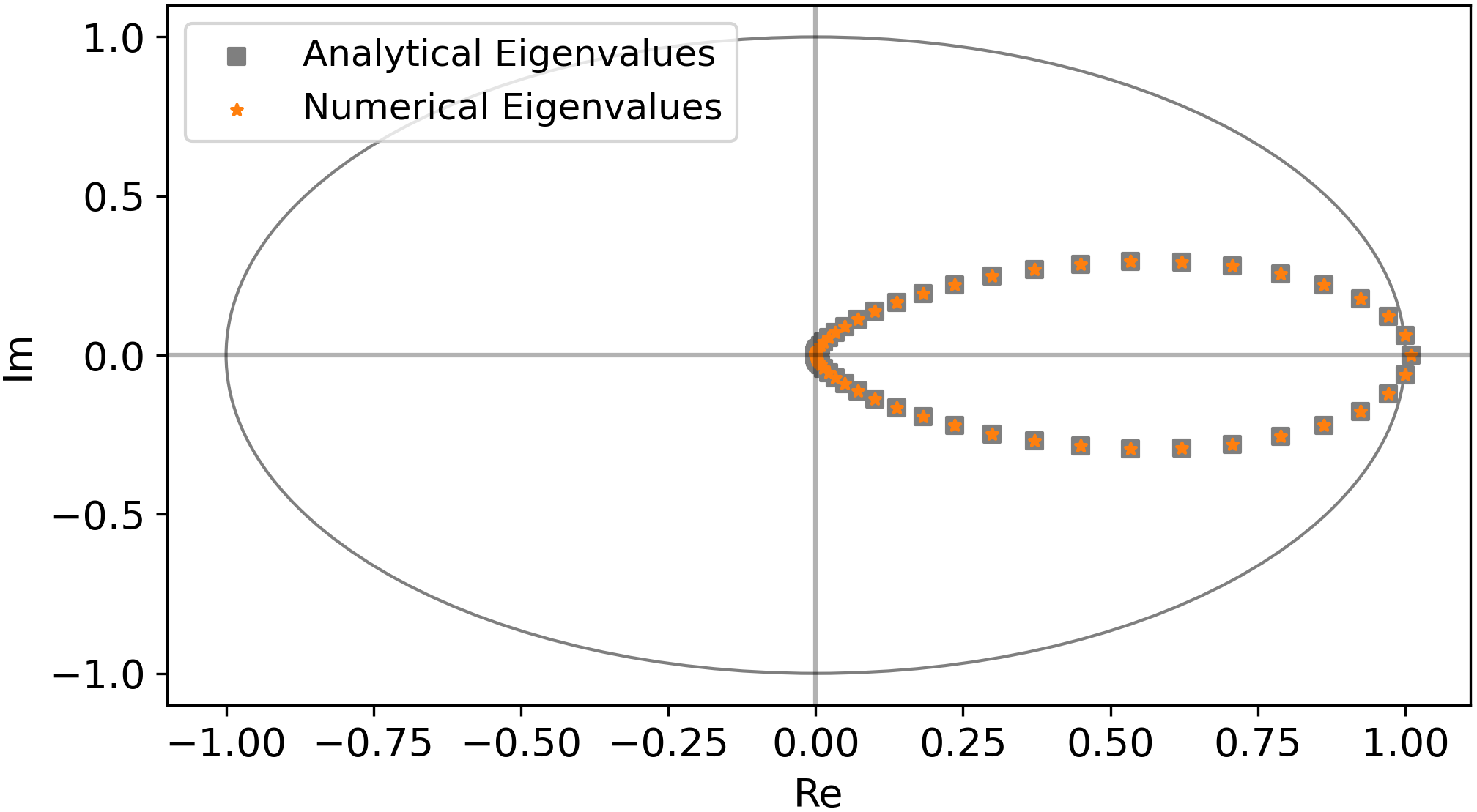
Figure 13: Analytical and numerical eigenvalues of the uncontrolled CDR equation

Figure 13 confirms the matching analytical and numerical eigenvalues of $A$. Our approach allows users to tune the system’s open-loop stability by choosing $\nu$, $c$, and $r$. For example, the presence of one unstable eigenvalue outside the unit circle in Figure 13 explains the growth of the solution to the CDR equation seen in Figure 3. By choosing a negative value for $r$, one can instead obtain an open-loop stable CDR equation environment. Lastly, we note that one can apply the same derivation process to the wave and Schrödinger equations.

3.2 Model-Based Controllers as Baselines

⬇

import controlgym as gym

if __name__ == "__main__":

env = gym.make("he1")

lqg = gym.controllers.LQG(env)

lqg.run()

gym.save(lqg)

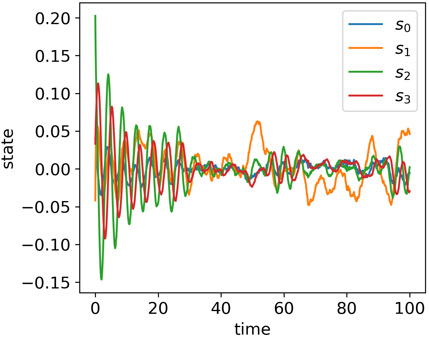
Figure 14: LQG controller applied to environment “he1”. Left: Python code snippet for setting up the environment and controller. Right: Plot of the system states against time.

In Figure 14, we show a code example of implementing the linear-quadratic-Gaussian (LQG) controller to the helicopter environment “he1”. In this example, we set the sampling time $\Delta t$ to be $0.1$ and construct the environment using the function call controlgym.make(). Other environments could be set up similarly with environment IDs from Tables 1-2 and optional keyword arguments. In addition to the LQG controller, we implement LQR and the state-feedback $H_{2}/H_{\infty}$ controllers in controlgym. For examples of applying baseline model-based controllers to linear PDE environments, we refer the readers to the example notebook file in our GitHub repository.

3.3 Model-Free RL Algorithms

⬇

import controlgym as gym

if __name__ == "__main__":

env = gym.make("he1")

ppo = gym.controllers.PPO(env,

actor_hidden_dim = 64,

critic_hidden_dim = 64, lr = 1e-5)

ppo.train(num_train_iter=100,

num_episodes_per_iter=64,

episode_length=100, sgd_epoch_num=4,

mini_batch_size=5, cov_param=0.05)

ppo.run()

gym.save(ppo)

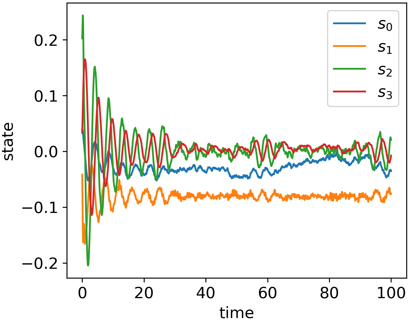
Figure 15: PPO controller applied to the helicopter environment “he1”

Other than the baseline model-based controllers, we also implement the proximal policy optimization (PPO) algorithm in controlgym. At the same time, all our environments support standard RL algorithms (Sutton et al., 2000; Kakade, 2002; Schulman et al., 2015, 2017; Mnih et al., 2016; Sutton and Barto, 2018), e.g., as seen in stable-baselines3 (Raffin et al., 2021).

We trained the PPO algorithm over 100 iterations, using the parameters detailed in the code snippet in Figure 15. Observations drawn from the graph on the right of Figure 15 reveal that the PPO controller, upon convergence, successfully steers three of the four state variables towards zero. However, one state variable settles at approximately $-0.1$, deviating from the target value, which is not ideal. We provide additional examples of applying PPO to a PDE environment and RL algorithms from stable-baselines3 to a linear control environment in our GitHub repository.

3.4 Generate Uncontrolled PDE Trajectories

In Figure 16, we show how to generate uncontrolled PDE trajectories (Figures 3-12) using a zero controller, exemplified through the CDR equation environment. This approach is instrumental for exploring the open-loop dynamics of PDEs, particularly in tuning physical parameters (cf., Section 3.1) and testing various initial conditions to identify the optimal experimental settings.

⬇

import controlgym as gym

if __name__ == "__main__":

env = gym.make("convection_diffusion_reaction")

zero = gym.controllers.Zero(env)

zero.run()

gym.save(zero)

Figure 16: Applying a zero controller to the CDR environment to evaluate the open-loop trajectory

4 Conclusion

We have presented controlgym, a library designed to support the research efforts of L4DC. The controlgym project facilitates a deeper investigation into the performance of RL algorithms, particularly focusing on their convergence, the stability and robustness of RL-based controllers, and the scalability of RL algorithms to systems with high and infinite state dimensionality.

The research of XZ, WM, and TB were supported in part by the US Army Research Laboratory (ARL) Cooperative Agreement W911NF-17-2-0181, in part by the Army Research Office (ARO) MURI Grant AG285. SM and MB were supported solely by MERL.

References

- Agarwal et al. (2019) Naman Agarwal, Brian Bullins, Elad Hazan, Sham Kakade, and Karan Singh. Online control with adversarial disturbances. In International Conference on Machine Learning, pages 111–119, 2019.
- Bou et al. (2023) Albert Bou, Matteo Bettini, Sebastian Dittert, Vikash Kumar, Shagun Sodhani, Xiaomeng Yang, Gianni De Fabritiis, and Vincent Moens. TorchRL: A data-driven decision-making library for PyTorch. arXiv preprint arXiv:2306.00577, 2023.
- Brockman et al. (2016) Greg Brockman, Vicki Cheung, Ludwig Pettersson, Jonas Schneider, John Schulman, Jie Tang, and Wojciech Zaremba. OpenAI Gym. arXiv preprint arXiv:1606.01540, 2016.
- Brunke et al. (2022) Lukas Brunke, Melissa Greeff, Adam W. Hall, Zhaocong Yuan, Siqi Zhou, Jacopo Panerati, and Angela P. Schoellig. Safe learning in robotics: From learning-based control to safe reinforcement learning. Annual Review of Control, Robotics, and Autonomous Systems, 5:411–444, 2022.
- Brunton and Noack (2015) Steven L Brunton and Bernd R Noack. Closed-loop turbulence control: Progress and challenges. Applied Mechanics Reviews, 67(5):050801, 2015.
- Bu et al. (2019a) Jingjing Bu, Afshin Mesbahi, Maryam Fazel, and Mehran Mesbahi. LQR through the lens of first order methods: Discrete-time case. arXiv preprint arXiv:1907.08921, 2019a.
- Bu et al. (2019b) Jingjing Bu, Lillian J Ratliff, and Mehran Mesbahi. Global convergence of policy gradient for sequential zero-sum linear quadratic dynamic games. arXiv preprint arXiv:1911.04672, 2019b.
- Bucci et al. (2019) Michele Alessandro Bucci, Onofrio Semeraro, Alexandre Allauzen, Guillaume Wisniewski, Laurent Cordier, and Lionel Mathelin. Control of chaotic systems by deep reinforcement learning. Proceedings of the Royal Society A, 475(2231):20190351, 2019.
- Callaham et al. (2023) Jared Callaham, Ludger Paehler, and Sam Ahnert. HydroGym. https://github.com/dynamicslab/hydrogym, 2023. Accessed: 2023-11-15.
- Chen and Hazan (2021) Xinyi Chen and Elad Hazan. Black-box control for linear dynamical systems. In Conference on Learning Theory, pages 1114–1143, 2021.
- Cox and Matthews (2002) Steven M Cox and Paul C Matthews. Exponential time differencing for stiff systems. Journal of Computational Physics, 176(2):430–455, 2002.
- Cross and Hohenberg (1993) Mark C Cross and Pierre C Hohenberg. Pattern formation outside of equilibrium. Reviews of modern physics, 65(3):851, 1993.
- Cui et al. (2023) Leilei Cui, Tamer Başar, and Zhong-Ping Jiang. A reinforcement learning look at risk-sensitive linear quadratic Gaussian control. In Learning for Dynamics and Control Conference, pages 534–546, 2023.
- Cvitanović et al. (2010) Predrag Cvitanović, Ruslan L Davidchack, and Evangelos Siminos. On the state space geometry of the kuramoto–sivashinsky flow in a periodic domain. SIAM Journal on Applied Dynamical Systems, 9(1):1–33, 2010.
- Dean et al. (2020) Sarah Dean, Horia Mania, Nikolai Matni, Benjamin Recht, and Stephen Tu. On the sample complexity of the linear quadratic regulator. Foundations of Computational Mathematics, 20(4):633–679, 2020.
- Degrave et al. (2022) Jonas Degrave, Federico Felici, Jonas Buchli, Michael Neunert, Brendan Tracey, Francesco Carpanese, Timo Ewalds, Roland Hafner, Abbas Abdolmaleki, Diego de Las Casas, et al. Magnetic control of tokamak plasmas through deep reinforcement learning. Nature, 602(7897):414–419, 2022.
- Duan et al. (2022) Jingliang Duan, Jie Li, Shengbo Eben Li, and Lin Zhao. Optimization landscape of gradient descent for discrete-time static output feedback. In American Control Conference, pages 2932–2937, 2022.
- Duan et al. (2023) Jingliang Duan, Wenhan Cao, Yang Zheng, and Lin Zhao. On the optimization landscape of dynamic output feedback linear quadratic control. IEEE Transactions on Automatic Control, 2023.
- Duan et al. (2016) Yan Duan, Xi Chen, Rein Houthooft, John Schulman, and Pieter Abbeel. Benchmarking deep reinforcement learning for continuous control. In International conference on machine learning, pages 1329–1338, 2016.
- Dulac-Arnold et al. (2020) Gabriel Dulac-Arnold, Nir Levine, Daniel J Mankowitz, Jerry Li, Cosmin Paduraru, Sven Gowal, and Todd Hester. An empirical investigation of the challenges of real-world reinforcement learning. arXiv preprint arXiv:2003.11881, 2020.
- Fazel et al. (2018) Maryam Fazel, Rong Ge, Sham M Kakade, and Mehran Mesbahi. Global convergence of policy gradient methods for the linear quadratic regulator. In International Conference on Machine Learning, pages 1467–1476, 2018.
- Furieri et al. (2020) Luca Furieri, Yang Zheng, and Maryam Kamgarpour. Learning the globally optimal distributed LQ regulator. In Learning for Dynamics and Control, pages 287–297, 2020.
- Gradu et al. (2020) Paula Gradu, John Hallman, Daniel Suo, Alex Yu, Naman Agarwal, Udaya Ghai, Karan Singh, Cyril Zhang, Anirudha Majumdar, and Elad Hazan. Deluca–a differentiable control library: Environments, methods, and benchmarking. Differentiable Computer Vision, Graphics, and Physics in Machine Learning (Neurips 2020 Workshop), 2020.
- Gravell et al. (2019) Benjamin Gravell, Peyman Mohajerin Esfahani, and Tyler Summers. Learning robust controllers for linear quadratic systems with multiplicative noise via policy gradient. arXiv preprint arXiv:1907.03680, 2019.
- Guo and Hu (2022) Xingang Guo and Bin Hu. Global convergence of direct policy search for state-feedback robust control: A revisit of nonsmooth synthesis with goldstein subdifferential. In 36th Conference on Neural Information Processing Systems, New Orleans, LA, Nov, volume 28, 2022.
- Hambly et al. (2021) Ben Hambly, Renyuan Xu, and Huining Yang. Policy gradient methods for the noisy linear quadratic regulator over a finite horizon. SIAM Journal on Control and Optimization, 59(5):3359–3391, 2021.
- Hu et al. (2023) Bin Hu, Kaiqing Zhang, Na Li, Mehran Mesbahi, Maryam Fazel, and Tamer Başar. Toward a theoretical foundation of policy optimization for learning control policies. Annual Review of Control, Robotics, and Autonomous Systems, 6:123–158, 2023.
- Jansch-Porto et al. (2022) Joao Paulo Jansch-Porto, Bin Hu, and Geir E Dullerud. Policy optimization for markovian jump linear quadratic control: Gradient method and global convergence. IEEE Transactions on Automatic Control, 68(4):2475–2482, 2022.
- Ju et al. (2022) Caleb Ju, Georgios Kotsalis, and Guanghui Lan. A model-free first-order method for linear quadratic regulator with sampling complexity. arXiv preprint arXiv:2212.00084, 2022.
- Kakade (2002) Sham M Kakade. A natural policy gradient. In Advances in Neural Information Processing Systems, pages 1531–1538, 2002.
- Kassam and Trefethen (2005) Aly-Khan Kassam and Lloyd N Trefethen. Fourth-order time-stepping for stiff pdes. SIAM Journal on Scientific Computing, 26(4):1214–1233, 2005.
- Keivan et al. (2022) Darioush Keivan, Aaron Havens, Peter Seiler, Geir Dullerud, and Bin Hu. Model-free synthesis via adversarial reinforcement learning. In American Control Conference, pages 3335–3341, 2022.
- L4DC (2023) L4DC. L4DC 2024 conference. https://l4dc.web.ox.ac.uk/, 2023. Accessed: 2023-11-15.
- Lale et al. (2022) Sahin Lale, Kamyar Azizzadenesheli, Babak Hassibi, and Animashree Anandkumar. Reinforcement learning with fast stabilization in linear dynamical systems. In International Conference on Artificial Intelligence and Statistics, pages 5354–5390, 2022.
- Leibfritz and Lipinski (2004) F Leibfritz and W Lipinski. COMPib 1.0–user manual and quick reference. Department of Mathematics, University of Trier, D–54286 Trier, Germany, Tech. Rep, 2004.
- Leibfritz (2004) Friedemann Leibfritz. COMPib, COnstraint Matrix-optimization Problem rary-a collection of test examples for nonlinear semidefinite programs, control system design and related problems. Dept. Math., Univ. Trier, Trier, Germany, Tech. Rep, 2004, 2004.
- Li et al. (2021) Yingying Li, Yujie Tang, Runyu Zhang, and Na Li. Distributed reinforcement learning for decentralized linear quadratic control: A derivative-free policy optimization approach. IEEE Transactions on Automatic Control, 67(12):6429–6444, 2021.
- Liang et al. (2018) Eric Liang, Richard Liaw, Robert Nishihara, Philipp Moritz, Roy Fox, Ken Goldberg, Joseph Gonzalez, Michael Jordan, and Ion Stoica. RLlib: Abstractions for distributed reinforcement learning. In International conference on machine learning, pages 3053–3062, 2018.
- Liu and Wang (2021) Xin-Yang Liu and Jian-Xun Wang. Physics-informed dyna-style model-based deep reinforcement learning for dynamic control. Proceedings of the Royal Society A, 477(2255):20210618, 2021.
- Malik et al. (2020) Dhruv Malik, Ashwin Pananjady, Kush Bhatia, Koulik Khamaru, Peter L Bartlett, and Martin J Wainwright. Derivative-free methods for policy optimization: Guarantees for linear quadratic systems. Journal of Machine Learning Research, 21(21):1–51, 2020.
- Mnih et al. (2016) Volodymyr Mnih, Adria Puigdomenech Badia, Mehdi Mirza, Alex Graves, Timothy Lillicrap, Tim Harley, David Silver, and Koray Kavukcuoglu. Asynchronous methods for deep reinforcement learning. In International Conference on Machine Learning, pages 1928–1937, 2016.
- Mohammadi et al. (2021) Hesameddin Mohammadi, Armin Zare, Mahdi Soltanolkotabi, and Mihailo R Jovanović. Convergence and sample complexity of gradient methods for the model-free linear–quadratic regulator problem. IEEE Transactions on Automatic Control, 67(5):2435–2450, 2021.
- Mowlavi et al. (2023) Saviz Mowlavi, Mouhacine Benosman, and Saleh Nabi. Reinforcement learning-based estimation for partial differential equations. arXiv preprint arXiv:2302.01189, 2023.
- Ozaslan et al. (2022) Ibrahim K Ozaslan, Hesameddin Mohammadi, and Mihailo R Jovanović. Computing stabilizing feedback gains via a model-free policy gradient method. IEEE Control Systems Letters, 7:407–412, 2022.
- Pan et al. (2018) Yangchen Pan, Amir-massoud Farahmand, Martha White, Saleh Nabi, Piyush Grover, and Daniel Nikovski. Reinforcement learning with function-valued action spaces for partial differential equation control. In International Conference on Machine Learning, pages 3986–3995. PMLR, 2018.
- Peitz et al. (2023) Sebastian Peitz, Jan Stenner, Vikas Chidananda, Oliver Wallscheid, Steven L Brunton, and Kunihiko Taira. Distributed control of partial differential equations using convolutional reinforcement learning. arXiv preprint arXiv:2301.10737, 2023.
- Perdomo et al. (2021) Juan C Perdomo, Jack Umenberger, and Max Simchowitz. Stabilizing dynamical systems via policy gradient methods. In Advances in Neural Information Processing Systems, pages 29274–29286, 2021.
- Raffin et al. (2021) Antonin Raffin, Ashley Hill, Adam Gleave, Anssi Kanervisto, Maximilian Ernestus, and Noah Dormann. Stable-baselines3: Reliable reinforcement learning implementations. The Journal of Machine Learning Research, 22(1):12348–12355, 2021.
- Rao and Yip (2018) Kamisetty Ramam Rao and Patrick C Yip. The Transform and Data Compression Handbook. CRC Press, 2018.
- Recht (2019) Benjamin Recht. A tour of reinforcement learning: The view from continuous control. Annual Review of Control, Robotics, and Autonomous Systems, 2:253–279, 2019.
- Schmid and Henningson (2001) Peter J Schmid and Dan S Henningson. Stability and Transition in Shear Flows. Springer, 2001.
- Schulman et al. (2015) John Schulman, Sergey Levine, Pieter Abbeel, Michael Jordan, and Philipp Moritz. Trust region policy optimization. In International Conference on Machine Learning, pages 1889–1897, 2015.
- Schulman et al. (2017) John Schulman, Filip Wolski, Prafulla Dhariwal, Alec Radford, and Oleg Klimov. Proximal policy optimization algorithms. arXiv preprint arXiv:1707.06347, 2017.
- Simchowitz and Foster (2020) Max Simchowitz and Dylan Foster. Naive exploration is optimal for online lqr. In International Conference on Machine Learning, pages 8937–8948, 2020.
- Simchowitz et al. (2020) Max Simchowitz, Karan Singh, and Elad Hazan. Improper learning for non-stochastic control. In Conference on Learning Theory, pages 3320–3436, 2020.
- Sutton and Barto (2018) Richard S Sutton and Andrew G Barto. Reinforcement learning: An introduction. MIT press, 2018.
- Sutton et al. (2000) Richard S Sutton, David A McAllester, Satinder P Singh, and Yishay Mansour. Policy gradient methods for reinforcement learning with function approximation. In Advances in Neural Information Processing Systems, pages 1057–1063, 2000.
- Tang et al. (2023) Yujie Tang, Yang Zheng, and Na Li. Analysis of the optimization landscape of linear quadratic Gaussian (LQG) control. Mathematical Programming, 2023. URL https://doi.org/10.1007/s10107-023-01938-4.
- Todorov et al. (2012) Emanuel Todorov, Tom Erez, and Yuval Tassa. Mujoco: A physics engine for model-based control. In 2012 IEEE/RSJ international conference on intelligent robots and systems, pages 5026–5033, 2012.
- Towers et al. (2023) Mark Towers, Jordan K. Terry, Ariel Kwiatkowski, John U. Balis, Gianluca de Cola, Tristan Deleu, Manuel Goulão, Andreas Kallinteris, Arjun KG, Markus Krimmel, Rodrigo Perez-Vicente, Andrea Pierré, Sander Schulhoff, Jun Jet Tai, Andrew Tan Jin Shen, and Omar G. Younis. Gymnasium, March 2023. URL https://zenodo.org/record/8127025.
- Trefethen (1996) Lloyd Nicholas Trefethen. Finite difference and spectral methods for ordinary and partial differential equations, 1996. URL http://people.maths.ox.ac.uk/trefethen/pdetext.html.
- Tsiamis et al. (2022) Anastasios Tsiamis, Ingvar Ziemann, Nikolai Matni, and George J Pappas. Statistical learning theory for control: A finite sample perspective. arXiv preprint arXiv:2209.05423, 2022.
- Tu and Recht (2019) Stephen Tu and Benjamin Recht. The gap between model-based and model-free methods on the linear quadratic regulator: An asymptotic viewpoint. In Conference on Learning Theory, pages 3036–3083, 2019.
- Tunyasuvunakool et al. (2020) Saran Tunyasuvunakool, Alistair Muldal, Yotam Doron, Siqi Liu, Steven Bohez, Josh Merel, Tom Erez, Timothy Lillicrap, Nicolas Heess, and Yuval Tassa. dm_control: Software and tasks for continuous control. Software Impacts, 6:100022, 2020. ISSN 2665-9638. URL https://www.sciencedirect.com/science/article/pii/S2665963820300099.
- Umenberger et al. (2022) Jack Umenberger, Max Simchowitz, Juan C Perdomo, Kaiqing Zhang, and Russ Tedrake. Globally convergent policy search over dynamic filters for output estimation. arXiv preprint arXiv:2202.11659, 2022.
- Vamvoudakis et al. (2021) Kyriakos G Vamvoudakis, Yan Wan, Frank L Lewis, and Derya Cansever. Handbook of reinforcement learning and control. Springer, 2021.
- Vignon et al. (2023) Colin Vignon, Jean Rabault, and Ricardo Vinuesa. Recent advances in applying deep reinforcement learning for flow control: Perspectives and future directions. Physics of Fluids, 35(3), 2023.
- Weng et al. (2022) Jiayi Weng, Huayu Chen, Dong Yan, Kaichao You, Alexis Duburcq, Minghao Zhang, Yi Su, Hang Su, and Jun Zhu. Tianshou: A highly modularized deep reinforcement learning library. Journal of Machine Learning Research, 23(267):1–6, 2022. URL http://jmlr.org/papers/v23/21-1127.html.
- Werner and Peitz (2023) Stefan Werner and Sebastian Peitz. Learning a model is paramount for sample efficiency in reinforcement learning control of pdes. arXiv preprint arXiv:2302.07160, 2023.
- Yang et al. (2020) Yunjie Yang, Yan Wan, Jihong Zhu, and Frank L Lewis. tracking control for linear discrete-time systems: model-free q-learning designs. IEEE Control Systems Letters, 5(1):175–180, 2020.
- Yang et al. (2019) Zhuoran Yang, Yongxin Chen, Mingyi Hong, and Zhaoran Wang. Provably global convergence of actor-critic: A case for linear quadratic regulator with ergodic cost. Advances in neural information processing systems, 32, 2019.
- Zeng et al. (2022) Kevin Zeng, Alec J Linot, and Michael D Graham. Data-driven control of spatiotemporal chaos with reduced-order neural ode-based models and reinforcement learning. Proceedings of the Royal Society A, 478(2267):20220297, 2022.
- Zhang et al. (2019) Kaiqing Zhang, Zhuoran Yang, and Tamer Basar. Policy optimization provably converges to nash equilibria in zero-sum linear quadratic games. Advances in Neural Information Processing Systems, 32, 2019.
- Zhang et al. (2020) Kaiqing Zhang, Bin Hu, and Tamer Başar. On the stability and convergence of robust adversarial reinforcement learning: A case study on linear quadratic systems. In Advances in Neural Information Processing Systems, pages 22056–22068, 2020.
- Zhang et al. (2021a) Kaiqing Zhang, Bin Hu, and Tamer Başar. Policy optimization for linear control with robustness guarantee: Implicit regularization and global convergence. SIAM Journal on Control and Optimization, 59(6):4081–4109, 2021a.
- Zhang et al. (2021b) Kaiqing Zhang, Xiangyuan Zhang, Bin Hu, and Tamer Başar. Derivative-free policy optimization for linear risk-sensitive and robust control design: Implicit regularization and sample complexity. In Advances in Neural Information Processing Systems, pages 2949–2964, 2021b.
- Zhang and Başar (2023) Xiangyuan Zhang and Tamer Başar. Revisiting LQR control from the perspective of receding-horizon policy gradient. IEEE Control Systems Letters, 7:1664–1669, 2023.
- Zhang et al. (2023a) Xiangyuan Zhang, Bin Hu, and Tamer Başar. Learning the Kalman filter with fine-grained sample complexity. In American Control Conference, pages 4549–4554, 2023a.
- Zhang et al. (2023b) Xiangyuan Zhang, Saviz Mowlavi, Mouhacine Benosman, and Tamer Başar. Global convergence of receding-horizon policy search in learning estimator designs. arXiv preprint arXiv:2309.04831, 2023b.
- Zhang et al. (2023c) Xiangyuan Zhang, Raj Kiriti Velicheti, and Tamer Başar. Learning minimax-optimal terminal state estimators and smoothers. In 22nd IFAC World Congress, pages 12391–12396, 2023c.
- Zhang et al. (2021c) Yufeng Zhang, Zhuoran Yang, and Zhaoran Wang. Provably efficient actor-critic for risk-sensitive and robust adversarial rl: A linear-quadratic case. In International Conference on Artificial Intelligence and Statistics, pages 2764–2772, 2021c.
- Zhao and You (2021) Feiran Zhao and Keyou You. Primal-dual learning for the model-free risk-constrained linear quadratic regulator. In Learning for Dynamics and Control, pages 702–714, 2021.
- Ziemann et al. (2022) Ingvar Ziemann, Anastasios Tsiamis, Henrik Sandberg, and Nikolai Matni. How are policy gradient methods affected by the limits of control? In Conference on Decision and Control, pages 5992–5999, 2022.