Compton scattering of electrons in the intergalactic medium

Abstract

This paper investigates the distribution and implications of cosmic ray electrons within the intergalactic medium (IGM). Utilizing a synthesis model of the extragalactic background, we evolve the spectrum of Compton-included cosmic rays. The energy density distribution of cosmic ray electrons peaks at redshift $z\approx 2$, and peaks in the $\sim$MeV range. The fractional contribution of cosmic ray pressure to the general IGM pressure progressively increases toward lower redshift. At mean density, the ratio of cosmic ray electron to thermal pressure in the IGM $P_{\rm CRe}/P_{\rm th}$ is 0.3% at $z=2$, rising to 1.0% at $z=1$, and 1.8% at $z=0.1$. We compute the linear Landau damping rate of plasma oscillations in the IGM caused by the $\sim$MeV cosmic ray electrons, and find it to be of order $\sim 10^{-6}\,\rm s^{-1}$ for wavenumbers $1.2\lesssim ck/\omega_{\rm p}\lesssim 5$ at $z=2$ and mean density (where $\omega_{\rm p}$ is the plasma frequency). This strongly affects the fate of TeV $e^{+}e^{-}$ pair beams produced by blazars, which are potentially unstable to oblique instabilities involving plasma oscillations with wavenumber $ck/\omega_{\rm p}\approx\sec\theta$ ($\theta$ being the angle between the beam and wave vector). Linear Landau damping is at least thousands of times faster than either pair beam instability growth or collisional effects; it thus turns off the pair beam instability except for modes with very small $\theta$ ($ck/\omega_{\rm p}\rightarrow 1$, where linear Landau damping is kinematically suppressed). This leaves open the question of whether the pair beam instability is turned off entirely, or can still proceed via the small-$\theta$ modes.

1 Introduction

Cosmic ray electrons are ubiquitous in the Universe. They are present locally near Earth (see Boezio et al. 2000; Adriani et al. 2011; Aguilar et al. 2019 for measurements down to GeV energies), and can now be measured down to low ($\sim$few MeV) energies beyond the heliopause (Stone et al., 2013; Cummings et al., 2016). Within the Milky Way’s interstellar medium (ISM), cosmic ray electrons are responsible for the principal sources of emission in radio (synchrotron emission) and contribute significantly to the diffuse gamma rays via inverse Compton and bremsstrahlung emission (see, e.g., Ackermann et al., 2012; Orlando & Strong, 2013; Acero et al., 2016) and are modeled in standard tools to predict radio and gamma ray emission (e.g. Orlando et al., 2018). On even larger scales, cosmic ray leptons are visible via radio haloes and relics in galaxy clusters (see Ferrari et al. 2008; Feretti et al. 2012; van Weeren et al. 2019 for reviews).

By volume, most of the Universe is filled with the intergalactic medium (IGM), and much remains unknown regarding the role of non-thermal components such as leptonic and hadronic cosmic rays and magnetic fields in the low-density IGM phases. Cosmic rays are generally understood to be accelerated in collisionless shocks (Axford et al., 1977; Bell, 1978; Blandford & Ostriker, 1978). Structure formation shocks, such as those at filaments, provide a natural site for accelerating cosmic ray electrons, and modern cosmological simulations of cosmic rays contain a source term based on fits to microphysical shock simulations (Pfrommer et al., 2017; Böss et al., 2023). Galactic winds could also advect cosmic rays into the IGM, or provide additional shocks for (re-)acceleration. Alternatively, cosmic rays could diffuse into the IGM, although the length scale over which they can diffuse is uncertain (Lacki, 2015). Nevertheless, most of the volume of the IGM is in voids that have been subjected at most to very weak shocks, e.g., from relaxation following reionization (Shapiro et al., 2004; Hirata, 2018). Diffusive acceleration in weaker shocks produces a much softer spectrum of cosmic rays: the phase space density declines with momentum as $f(p)\propto p^{-4/(1-{\cal M}^{-2})}$ instead of $f(p)\propto p^{-4}$ (where $p$ is the momentum and ${\cal M}$ is the Mach number), whereas to produce an electron with a collisional momentum loss rate $(d\ln p/dt)_{\rm coll}=H(z)$ one must reach quasi-relativistic momenta, e.g., $p\approx 1.4m_{e}c$ at $z=2$ and mean density. Furthermore, this spectrum only exists if non-thermal seed electrons are present on which diffusive shock acceleration can act: this “injection problem” for electrons, and the circumstances under which it is solved, are a subject of current research (e.g. Amano & Hoshino, 2010; Riquelme & Spitkovsky, 2011; Kobzar et al., 2021; Shalaby et al., 2022). Electrons may also be present as secondary cosmic rays, however low Mach number shocks in plasmas with weak magnetic fields may not always efficiently accelerate protons or He ions (Ha et al., 2018).

It is therefore of interest to investigate sources of cosmic ray electrons that could apply in the full volume of the IGM. Gamma rays produced by sources such as active galactic nuclei (AGN) are neutral and thus can propagate freely into the IGM. While the Universe is mostly transparent to $\sim$MeV gamma rays, a small percentage of them will interact in the IGM via Compton scattering:

$$\gamma+e^{-}({\rm th})\rightarrow\gamma+e^{-}({\rm cr}),$$ (1)

where “th” and “cr” denote thermal and cosmic ray electrons, respectively. Compton scattering of the X-ray background is a potential source of heating in the IGM (Madau & Efstathiou, 1999), which is most important in low-density regions where photoionization heating is weaker (Haardt & Madau, 2012). Compton scattering of X-rays will produce non-relativistic recoil electrons that thermalize their energy in a cosmologically short time, but gamma ray photons in the $\sim$few MeV range can produce quasi-relativistic electrons ($p/m_{e}c$ of order unity). At IGM densities and low redshift ($z\lesssim 5$), these quasi-relativistic electrons can survive for cosmologically long timescales, since neither collisional losses nor inverse Compton cooling via the cosmic microwave background (CMB: important for much higher energies) are fast. This provides a “guaranteed” source of cosmic ray electrons in the IGM. The central calculation in this paper is to take a synthesis model of the extragalactic background and evolve the spectrum of Compton-included cosmic rays in the IGM.

There are several consequences for a ubiquitous cosmic ray electron population everywhere in the IGM. In this paper, we focus our detailed calculations on the most spectacular result: cosmic rays modify the dispersion relation of plasma waves in the IGM. This affects the fate of the TeV pair beams produced by blazars via

$$\gamma({\rm TeV})+\gamma({\rm EBL})\rightarrow e^{+}+e^{-},$$ (2)

where “$\gamma$(TeV)” denotes a TeV photon emitted by a blazar and “EBL” denotes the typically $\sim$eV extragalactic background light. These pair beams can cool via inverse Compton scattering, but it has also been proposed that they drive an instability of plasma oscillations that could disrupt the beam and lead to an additional heating source in the IGM (Broderick et al., 2012; Chang et al., 2012). It has been debated whether detuning due to density (and hence plasma frequency) gradients (Miniati & Elyiv, 2013) or transfer of energy to longer-wavelength plasma oscillation modes (Sironi & Giannios, 2014) stops the instability from growing (but see, e.g., Schlickeiser et al. 2013; Chang et al. 2014; Shalaby et al. 2018 for counterarguments). Limits on the $\sim 100$ GeV gamma rays produced by inverse Compton process further motivate understanding whether the plasma instability mechanisms can cool pair beams (e.g. Blanco et al., 2023). We will show in this paper that the $\sim$MeV electrons cause linear Landau damping of plasma oscillations; the damping rates can be thousands of times faster than would occur for a purely thermal plasma. This suppresses the plasma instabilities in most (but not quite all) of the relevant parameters space.

This paper is organized as follows: In Section 2, we present the formalism of electron cosmic rays. In Section 3, we discuss the different components of the model. Section 4 provides a numerical solution. We present the results and contribution of the electron cosmic rays to the IGM pressure, energy density, and plasma oscillation damping rate in Section 5. Finally, Section 6 discusses some of the other potential implications of the cosmic ray electrons that might be explored in future work.

2 Conventions and conversions

We want to construct a model to represent the Compton-scattered electron cosmic ray distribution within the Intergalactic Medium (IGM). To start, it is pivotal to parameterize the cosmic ray spectrum. An approach to achieve this is to define $N(E)$ as the number of electrons per unit physical volume per unit energy $E=m_{e}c^{2}(\gamma-1)$ [units: cm^-3 erg^-1]. Then there is an energy content per baryon in cosmic rays of $\int EN(E)\,dE/n_{b}$, where $n_{b}$ is the physical baryon density.

Under the assumptions of neglecting diffusion and the absence of a shock crossing, the governing evolution equation can be stated as:

$$\frac{\partial}{\partial t}N(E)= - \theta N(E)+\frac{1}{3}\theta\frac{\partial}{\partial E}\left[\frac{E(E+2m_{e}c^{2})}{E+m_{e}c^{2}}N(E)\right]-\frac{\partial}{\partial E}\left[\left.\frac{dE}{dt}\right|_{\rm loss}N(E)\right]$$ (3)

$$+ n_{e,\rm tot}\int_{2E}^{\infty}c\beta^{\prime}\frac{d\sigma_{\rm M}(E|E^{\prime})}{dE}N(E^{\prime})dE^{\prime}+S(E,t),$$

where $\theta=3H-d\ln\Delta/dt$ is the divergence of the baryon velocity and $\Delta$ is the relative overdensity. The first two terms in this equation account for the dilution of the density and the momentum alteration for adiabatic expansion. When adiabatic expansion induces a stretch in the de Broglie wavelength of a particle by a factor of $\Delta\lambda/\lambda$, the consequent energy decrease is given by $\Delta E=-\Delta\lambda/\lambda\times E(E+2m_{e}c^{2})/(E+m_{e}c^{2})$. The term $(dE/dt)|_{\rm loss}$ represents energy loss rate. Moreover, $\sigma_{\rm M}(E|E^{\prime})\,dE$ represents the Møller scattering cross section for an electron of energy $E^{\prime}$ to produce a secondary electron of energy between $E$ and $E+dE$. Lately, $S(E,t)$ is defined as the source term.

Within the confines of our computational model, we use the Centimeter-Gram-Second (CGS) unit system, although the outputs can be translated into eV-based units to facilitate more intuitive interpretation. In the CGS framework, the electron mass is represented as $m_{e}c^{2}=8.187\times 10^{-7}\,$erg. Furthermore, all cross section are expressed in terms of the classical electron radius, denoted by $r_{0}=2.818\times 10^{-13}\,$cm.

Electrons will be described by their kinetic energy, symbolized as $E$. In relation to this kinetic energy, the Lorentz factor and the velocity, when expressed as a fraction of the speed of light, are described as follows:

$$\gamma=\frac{E}{m_{e}c^{2}}+1{\rm~{}~{}~{}and~{}~{}~{}}\beta=\frac{\sqrt{E(E+2m_{e}c^{2})}}{E+m_{e}c^{2}}.$$ (4)

We use the cosmological model from Planck Collaboration et al. (2020): $H_{\rm 0}=67.4\,\rm km\,s^{-1}Mpc^{-1}$, $\Omega_{\rm m}=0.315$ and $\Omega_{\rm b}\rm h^{2}=0.0224$.

3 Model ingredients

3.1 Density evolution

Our model for the gas density evolution is a spherical over- (or under-) density in a $\Lambda$CDM background universe. Due to Birkhoff’s theorem, a uniform spherical overdensity has a radius that satisfies the usual Friedmann equation (Peebles, 1967). Writing the radius as $a\xi$, where $a$ is the scale factor and the overdensity is $\Delta=\xi^{-3}$, the second-order Friedmann equation is

$$\frac{d^{2}}{dt^{2}}(a\xi)=-\frac{\Omega_{m}H_{0}^{2}}{2(a\xi)^{2}}+\frac{1}{2}(1-\Omega_{m})H_{0}^{2}a\xi$$ (5)

where the first term comes from the matter density and the second from the cosmological constant. It can be transformed into

$$\ddot{\xi}=-2H\dot{\xi}+\frac{\Omega_{m}H_{0}^{2}}{2a^{3}}\left(\xi-\xi^{-2}\right).$$ (6)

Here $H=d(\ln a)/dt$ is the Hubble rate. We initialize this equation at high redshift with $\xi=1-a\delta_{\rm lin}/3$ and $\dot{\xi}=-aH\delta_{\rm lin}/3$, where $\delta_{\rm lin}$ is the linear overdensity with the growth function scaled out, and evolve it to low redshift with a leapfrog scheme. $\delta_{\rm lin}$ = 0 means mean density, $\delta_{\rm lin}<$ 0 means underdensity, and $\delta_{\rm lin}>$ 0 means overdensity.

3.2 Source term

The source term $S(E,t)$ in Eq. (3) represents the rate of production of Compton-scattered electrons per unit physical volume per unit energy. It can be expressed in terms of the extragalactic background intensity as

$$S(E,t)=n_{e,\rm tot}\int_{E_{\gamma,\rm min}}^{\infty}\frac{d\sigma_{\rm KN}(E|E_{\gamma})}{dE}\frac{4\pi J(E_{\gamma})}{E_{\gamma}}dE_{\gamma},$$ (7)

where $J(E_{\gamma})=J_{\nu}/h$ is the background intensity at photon energy $E_{\gamma}=h\nu$. For $J_{\nu}$, we use the fiducial (“Q18”) model in Khaire & Srianand (2019) and interpolate the EBL specific intensity via a 4-nearest point method. We also use the model in Haardt & Madau (2012) for comparison in the discussion. The minimum photon energy to produce a recoil electron of energy $E$ is

$$E_{\gamma,\rm min}=\frac{1}{2}\left[E+\sqrt{E(E+2m_{e}c^{2})}\right],$$ (8)

and the Klein-Nishina cross section is

$$\frac{d\sigma_{\rm KN}(E|E_{\gamma})}{dE}=\pi r_{0}^{2}\frac{m_{e}c^{2}}{E_{\gamma}(E_{\gamma}-E)}\left[2+\frac{E^{2}}{E_{\gamma}^{2}}-2\frac{E}{E_{\gamma}}-2\frac{m_{e}c^{2}E}{E_{\gamma}^{2}}+\frac{(m_{e}c^{2})^{2}E^{2}}{E_{\gamma}^{3}(E_{\gamma}-E)}\right].$$ (9)

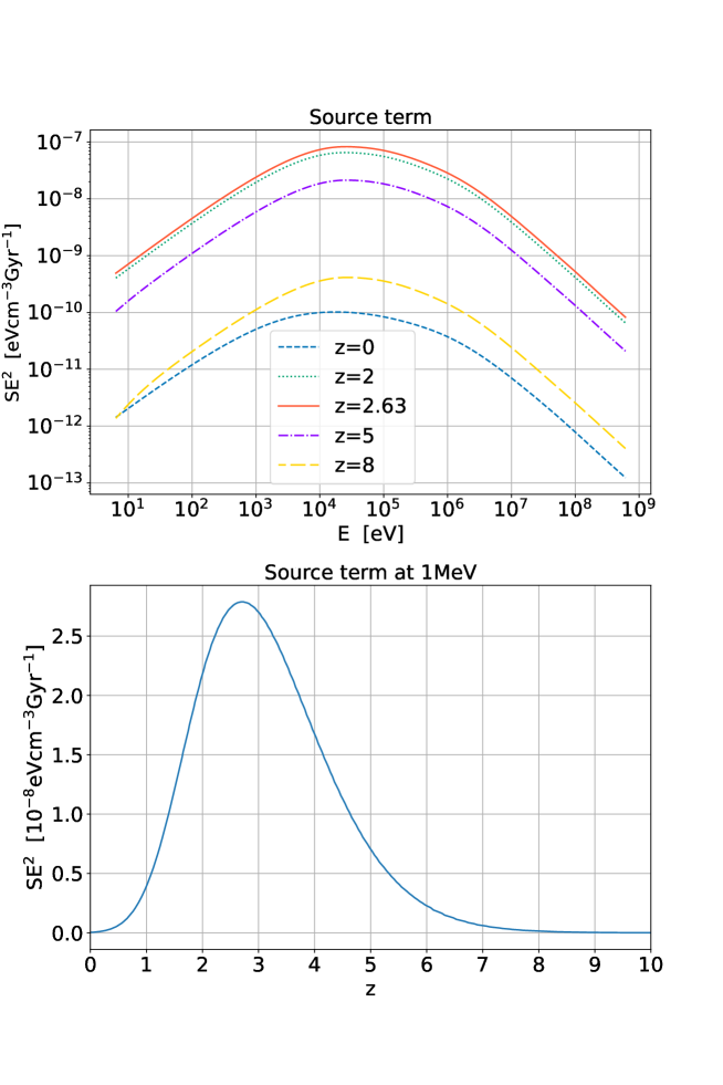
Figure 1: Top: The source terms at redshift $z$ = 0, 2, 2.63, 5, and 8 are labeled accordingly. Bottom: The production rate of 1 MeV electrons at different redshift. These source terms exhibit an increasing trend from $z$ = 15 to $z$ = 3, followed by a decrease from $z$ = 2 to $z$ = 0. Furthermore, they reach their peak around $z\approx$ 2 to 3.

The top panel of figure 1 illustrates the source terms at redshift $z$ = 0, 2, 2.63, 5, and 8. In our comprehensive results, these source terms exhibit an increasing trend from $z$ = 15 to $z$ = 3, followed by a decrease from $z$ = 2 to $z$ = 0, and reach their peak around $z\approx$ 2 to 3. The bottom panel of figure 1 illustrates one example of how source term evolving with redshift for 1 MeV electrons.

The principal source of model uncertainty here — and generally in this paper — is the extragalactic background in the $\sim$MeV range. The integrated background near Earth was measured by the Solar Maximum Mission (Watanabe et al., 2000) and Compton Gamma Ray Observatory (Weidenspointner et al., 2000). Khaire & Srianand (2019) adjusted the parameters of their Type 2 quasar spectral energy distribution (SED) to match the observed background. However, other sources may also contribute to the MeV background, including supernovae and radioactive and cosmic ray-induced processes in the ISM of galaxies; model predictions for these have ranged from a few to $\sim 10\%$ of the observed background (Iwabuchi & Kumagai, 2001; Strigari et al., 2005; Lacki et al., 2014). Although it is reasonable to expect that the MeV contribution would follow the overall redshift evolution of both star formation and AGN, peaking at “Cosmic Noon” and then declining toward the present day, unresolved background measurements cannot definitively establish whether this is the case. Finally, Khaire & Srianand (2019) present a “point estimate,” and $\sim$MeV backgrounds a factor of a few lower would also provide an acceptable fit.

3.3 Energy losses by relativistic electrons

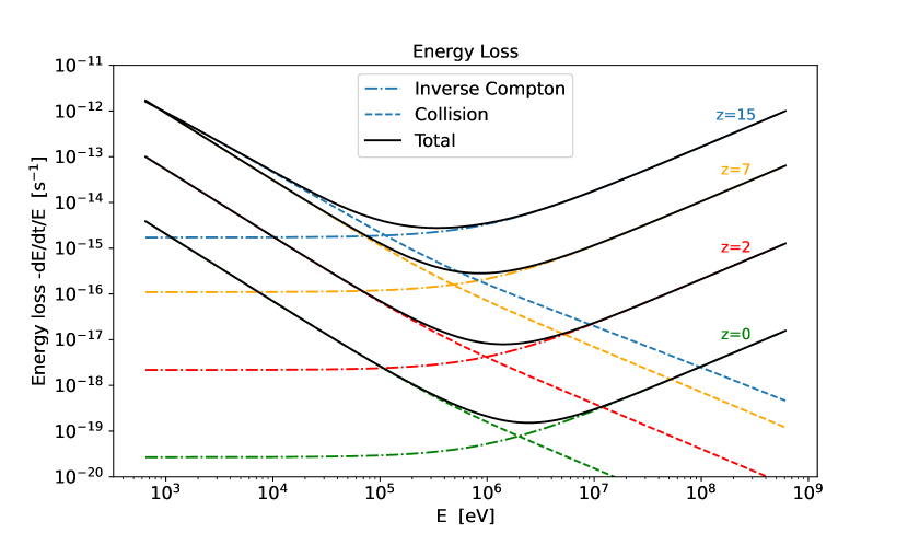
Figure 2: The energy loss due to inverse-Compton cooling (dot-dashed line), collision (dashed line), and the total energy loss (solid line) at the mean density for redshift $z=15$, 7, 2, and 0. As the redshift decreases, the energy loss rate also decreases. At lower electron energies ($\leq$ MeV), the dominant energy loss mechanism is collisional loss, whereas at higher electron energy levels, inverse-Compton cooling dominates the overall energy loss. Note the small change in slope at low $E$ from $z=15$ to $z=7$ due to reionization.

Electrons of the $\sim$MeV energy range in the intergalactic medium lose energy by two major mechanisms: inverse Compton cooling, and collisional losses (which include both free electrons in the plasma as well as collisions with bound electrons in H⁰, He⁰, and He⁺).

The inverse Compton loss can be computed using standard formulae. The expression of Jones (1965, Eqs. 16,20) gives, in the Thomson scattering limit $k_{\rm B}T_{\rm CMB}\gamma\ll m_{e}c^{2}$ where we may keep only the leading term in the infinite sum,

$$-\left\langle\frac{d\gamma}{dt}\right\rangle=\frac{32}{9}\pi r_{0}^{2}\frac{a_{\rm R}T_{\rm CMB}^{4}}{m_{e}c}\beta^{2}\gamma^{2},$$ (10)

where $r_{0}$ is the classical electron radius and $a_{\rm R}$ is the radiation constant. Written in terms of energy, this is

$$\left.\frac{dE}{dt}\right|_{\rm inv.~{}Compton}=-\frac{32\pi r_{0}^{2}a_{\rm R}T_{\rm CMB}^{4}}{9m_{e}c}\left(2+\frac{E}{m_{e}c^{2}}\right)E.$$ (11)

The energy loss due to collisions with free electrons in an ionized plasma can be computed using the standard formula (Rohrlich & Carlson, 1954; Uehling, 1954):

$$\left.\frac{dE}{dt}\right|_{\rm coll.,~{}free}=-\frac{2\pi n_{e}r_{0}^{2}m_{e}c^{3}}{\beta}\left[\ln\frac{E^{2}}{I^{2}}+\ln\left(1+\frac{\tau}{2}\right)+F^{-}-\delta\right],$$ (12)

where $n_{e}$ is the electron density. The high momentum transfer part of the energy loss, computed using the Møller (1932) scattering formula, is

$$F^{-}=(1-\beta^{2})\left[1+\frac{\tau^{2}}{8}-(2\tau+1)\ln 2\right],$$ (13)

and $\tau=E/m_{e}c^{2}$. For a plasma, the mean excitation energy $I$ is the plasma frequency $\omega_{p}$:

$$I=\hbar\omega_{p},~{}~{}~{}\omega_{p}=c\sqrt{4\pi r_{0}n_{e}}.$$ (14)

The density correction is given by the theory of Fano (1956, 1963), with $\Im[-1/\epsilon]=\frac{\pi}{2}\omega_{p}\delta_{\rm D}(\omega-\omega_{p})$ and $\ell=\omega_{p}\beta\gamma$:

$$\delta=2\ln\gamma-\beta^{2}.$$ (15)

This combines to give

$$\left.\frac{dE}{dt}\right|_{\rm coll.,~{}free}=-\frac{2\pi n_{e}r_{0}^{2}m_{e}c^{3}}{\beta}\left\{\ln\frac{E^{2}}{4\pi\hbar^{2}c^{2}r_{0}n_{e}}+\ln\left(1+\frac{\tau}{2}\right)+(1-\beta^{2})\left[1+\frac{\tau^{2}}{8}-(2\tau+1)\ln 2\right]-2\ln\gamma+\beta^{2}\right\}.$$ (16)

Note the presence of the usual Coulomb logarithm factor, as generally occurs in energy loss calculations.

If atoms with bound electrons (H⁰, He⁰, or He⁺) are present, then we should also take into account collisional losses with these species. The collisional loss rate is given by a modified version of Eq. (12) without a density correction:

$$\left.\frac{dE}{dt}\right|_{\rm coll.,~{}bound}=-\frac{2\pi r_{0}^{2}m_{e}c^{3}}{\beta}\sum_{{\rm species}~{}X}N_{e,X}n_{X}\left[\ln\frac{E^{2}}{I_{X}^{2}}+\ln\left(1+\frac{\tau}{2}\right)+F^{-}\right],$$ (17)

where $n_{X}$ is the number density of species $X$; $N_{e,X}$ is the number of bound electrons (1 for H⁰ or He⁺, or 2 for He⁰); and $I_{X}$ is the geometric mean excitation energy for species $X$ (15.0 eV for H⁰; 42.3 eV for He⁰; and 59.9 eV for He⁺).

We assume that hydrogen (H) undergoes complete ionization instantaneously at $z$ = 8, and helium (He) ionized into He⁺ completely at $z$ = 8 and experiences complete ionization instantaneously at $z$ = 3. While the ionization of H and He is a graduation processes, we simplify it by assuming instantaneous ionization. This assumption is reasonable because H is fully ionized around $z$ = 6, when cosmic rays are still not abundant. Similarly, although He reionization happens in the presence of abundant cosmic rays, the contribution of it to the overall electron population is only a few percent. Consequently, the simplicity of the instant ionization model does not significantly differ from more complex models.

Figure 2 displays the energy loss due to inverse-Compton cooling, collisions, and the total energy loss at mean density for redshift $z$ = 0, 2, 7, and 15. The energy loss rate demonstrates a decreasing trend as the redshift decreases. Notably, for electrons in lower energy levels ($\leq$ MeV), collisional loss stands out as the primary energy loss mechanism. Conversely, for electrons in higher energy levels, inverse-Compton cooling plays a dominant role in the overall energy loss.

3.4 Secondary electrons

The Møller scattering differential cross section to produce a secondary electron of energy $E$ from a primary of energy $E^{\prime}$ is (see, e.g., Berger & Seltzer 1982, Eq. 2.15):

$$\frac{d\sigma_{\rm M}(E|E^{\prime})}{dE}=\frac{2\pi r_{0}^{2}m_{e}c^{2}(m_{e}c^{2}+E^{\prime})^{2}}{E^{\prime}(2m_{e}c^{2}+E^{\prime})E^{2}}\left[1+\frac{E^{2}}{(E^{\prime}-E)^{2}}+\frac{E^{2}}{(m_{e}c^{2}+E^{\prime})^{2}}-\frac{m_{e}c^{2}(m_{e}c^{2}+2E^{\prime})E}{(m_{e}c^{2}+E^{\prime})^{2}(E^{\prime}-E)}\right]$$ (18)

with limits $E<E^{\prime}/2$ since we consider the “secondary” electron to be the one with lower energy (electrons are identical particles so this is a labeling convention).

4 Numerical solution

Equation (3) is a partial differential equation for $N(E,t)$ with two independent variables, $E$ and $t$. As redshift $z$ is more commonly used in cosmology, we can convert Equation (3) to $z$ format by

$$\frac{\partial}{\partial z}N(E,z)=\frac{dt}{dz}\frac{\partial N(E,t)}{\partial t}=-\frac{1}{(1+z)H(z)}\frac{\partial N(E,t)}{\partial t}.$$ (19)

This can be re-written in the form

$$\frac{\partial}{\partial z}N(E,z)=A_{1}(z)N(E,z)+\frac{\partial}{\partial E}[A_{2}(E,z)N(E,z)]+\int_{2E}^{\infty}A_{3}(E,E^{\prime},z)N(E^{\prime},z)dE^{\prime}+S_{z}(E,z),$$ (20)

where the coefficients $A_{1}$, $A_{2}$, $A_{3}$, and $S_{z}$ have the indicated dependences and are given by

$$A_{1}(z) = \frac{\theta}{(1+z)H(z)},$$

$$A_{2}(E,z) = -\frac{1}{(1+z)H(z)}\left[\frac{1}{3}\theta\frac{E(E+2m_{e}c^{2})}{E+m_{e}c^{2}}-\left.\frac{dE}{dt}\right|_{\rm loss}\right],$$

$$A_{3}(E,E^{\prime},z) = -\frac{1}{(1+z)H(z)}n_{e,\rm tot}\ c\beta^{\prime}\frac{d\sigma_{\rm M}(E|E^{\prime})}{dE},~{}~{}{\rm and}$$

$$S_{z}(E,z) = -\frac{S(E,t)}{(1+z)H(z)}.$$ (21)

To integrate Eq. (20), we discretize the energy axis into $m$ energy bins with logarithmically spaced energies $\{E_{i}\}_{i=0}^{m-1}$ and widths $\Delta E_{i}=E_{i+1/2}-E_{i-1/2}$. We track the number density of cosmic ray electrons $n_{i}(z)=N(E_{i},z)\Delta E_{i}$ (units: cm^-3) in each bin, and choose the following form:

$$\frac{dn_{i}(z)}{dz}=A_{1}(z)n_{i}(z)+A_{2}(E_{i+{1}/{2}},z)\frac{n_{i+1}(z)}{\Delta E_{i+1}}-A_{2}(E_{i-{1}/{2}},z)\frac{n_{i}(z)}{\Delta E_{i}}+\sum_{j:E_{j}\geq 2E_{i}}A_{3}(E_{i},E_{j},z)n_{j}(z)+S_{z}\Delta E_{i}.$$ (22)

There are several possible discretizations of the $A_{2}$ term: the version using $n_{i+1}(z)$ as chosen here, an alternative using $n_{i-1}(z)$, or a symmetric version using both. This version rigorously enforces that information flows only from higher to lower energy bins, and it is stable for the case of electrons losing energy ($A_{2}<0$).

Writing the $n_{i}$ as a length-$m$ column vector ${\boldsymbol{n}}$, Eq. (22) can be cast in the form

$$\frac{\partial\boldsymbol{n}}{\partial z}={\bf M}{\boldsymbol{n}}+{\boldsymbol{s}},$$ (23)

where the source vector ${\boldsymbol{s}}$ has components $s_{i}=S_{z}(E_{i},z)\Delta E_{i}$ and ${\bf M}$ is an $m\times m$ upper-triangular matrix.

We solve this using the backward Euler method:

$${\boldsymbol{n}}(z_{j+1})\approx[{\bf I}_{m\times m}-(z_{j+1}-z_{j}){\bf M}]^{-1}[{\boldsymbol{n}}(z_{j})+(z_{j+1}-z_{j}){\boldsymbol{s}}(z_{j+1})],$$ (24)

which allows us to inductively determine ${\boldsymbol{n}}(z_{1})$ from ${\boldsymbol{n}}(z_{0})$; then we can find ${\boldsymbol{n}}(z_{2})$ and so on. Since we integrate forward in time, $z_{j+1}-z_{j}<0$. We initialize with ${\boldsymbol{n}}(z_{0})=0$ at $z_{0}=15$. After finding $n_{i}(z_{j})$, we can divide by $\Delta E_{i}$ to get $N(E_{i},z_{j})$.

5 Results

5.1 Implication for energy and pressure balance in the IGM

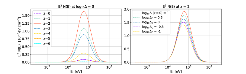
Figure 3: Energy density distribution of electrons across different energy bins. Left: Distribution at mean density for redshift $z=0...6$, as labeled. It peaks at $z=2$, and then declines, following the overall evolution of AGN emissivity. Right: Distribution at $z=2$ under different over- or under-densities. The curves are labeled by the value of $\log_{10}\Delta$ at the present epoch (all were closer to mean density at $z=2$). As the matter density increases, the energy density of electrons also rises. In all cases, the energy density of electrons peaks at around the MeV energy level.

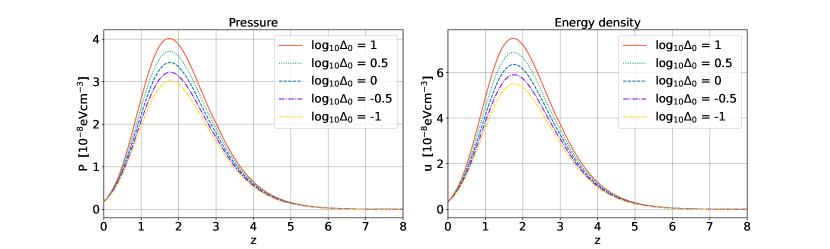
Figure 4: The energy density (left) and pressure (right) of electron cosmic rays for different matter over- or under-densities, as labeled. In both plots, we observe an increasing trend from $z$ = 0 to $z\approx$ 2, followed by a decrease as z increases, approaching values close to 0 before $z\approx$ 6. Furthermore, both the energy density and pressure exhibit higher value for higher matter density settings.

The total energy density from the electron cosmic rays is

$$u_{\rm CRe}=\int EN_{e}(E,z)dE,$$ (25)

and the pressure is given by the usual special relativistic result:

$$P_{\rm CRe}=\frac{1}{3}\int E\frac{E+2m_{e}c^{2}}{E+m_{e}c^{2}}N_{e}(E,z)dE.$$ (26)

Figure 3 depicts the energy density distribution of electrons across various energy bins. The left panel presents the distribution at mean density for redshifts $z=6$ down through $z=0$. The electron energies exhibit an increasing trend from $z=6$ to $z=2$, and then decreases toward lower redshift, consistent with the source distribution shown in Figure 1.

For the right panel, we focus on the snapshots at $z=2$ and illustrate the distribution at different overdensities. As the matter density increases, the energy density of electrons also rises, which is expected given that the ambient electrons are the targets that are Compton-scattered to produce cosmic rays. At lower energies, the curves converge because both the source and collisional energy losses are proportional to density. Notably, in all cases, the energy density of electrons peaks in the 0.1–1 MeV energy range. This finding aligns with Figure 2, which shows that energy losses by electrons are minimized in this range.

Figure 4 displays the energy density (left) and pressure (right) of electron cosmic rays as a function of redshift for various matter over- or under-density configurations. In both plots, we observe an increasing trend until $z\sim 1.7$, followed by a rapid decline toward $z=0$. This pattern is consistent with the findings in Figure 1 and the left plot of Figure 3. We should remember that these are physical energy densities and pressures, and thus the overall expansion of the Universe contributes to the low-$z$ decline: the $\sim$MeV photons emitted at Cosmic Noon are still present as an extragalactic background, but by $z\lesssim 1$ they have been diluted and redshifted. Furthermore, both the energy density and pressure are larger in overdensities, as depicted in the bottom plot of Figure 3.

Figure 5: The temperature profile (top), IGM thermal pressure (middle), and the pressure comparison (bottom) with redshift for different overdensity as labeled. The temperature experiences a sudden increase at $z$ = 3 (observed towards $z$ = 0) due to the instantaneously ionization of He ii. Which is also responsible for the rigid bump for the other two panels. In general, the temperature drops toward lower redshift, and higher overdensity corresponds to higher temperature profile (a “normal” temperature-density relation). The fractional contribution of cosmic ray pressure to the general IGM pressure progressively increases toward lower redshifts (again, with a small perturbation at $z=3$ due to helium reionization), and $P_{\rm CR}/P_{\rm th}$ is also largest in the low density regions (where the energy range over which cosmic ray electrons can survive without collisional cooling is largest).

To illustrate the additional pressure introduced by the MeV electron cosmic ray in the IGM, we model the thermal and pressure evolution of IGM. The temperature evolution of IGM gas is described by the following equation (Hui & Gnedin, 1997):

$$\frac{dT}{dt}=-2HT+\frac{2T}{3\Delta}\frac{d\Delta}{dt}-\frac{T}{n_{\rm tot}}\frac{dn_{\rm tot}}{dt}+\frac{2}{3k_{\rm B}n_{\rm tot}}\frac{dQ}{dt}$$ (27)

where $n_{\rm tot}$ is the total number density of free baryonic particles, $k_{\rm B}$ is the Boltzmann constant. The term $dQ/dt$ encodes the heating and cooling processes in the IGM and in this work we follow the modeling details in Upton Sanderbeck et al. (2016). The fiducial reionization scenario we choose is that H i reionization happens instantly at $z=8$, heating the gas to $T_{0}=2\times 10^{4}\,K$, and that He ii reionization happens at $z=3$ also instantaneously heats IGM through photoheating. We then calculate the thermal pressure of IGM using the ideal gas law, $P_{\rm th}(z)=n_{\rm tot}(z)k_{\rm B}T(z)$.

Figure 5 illustrates the temperature profile, fiducial IGM pressure, and the evolution of pressure ratio of MeV electron CR to IGM with respect to redshift for different overdensity settings. The temperature experiences a sudden increase at $z$ = 3 (observed towards $z$ = 0) due to the instantaneously ionization of He ii. Generally, the temperature drops from $z$ = 15 to $z$ = 0, and higher overdensity corresponds to higher temperature profile. The general IGM pressure exhibits a decrease from $z$ = 15 to $z$ = 0, with higher overdensity resulting in higher pressure. Moreover, the contribution of cosmic ray pressure to the general IGM pressure progressively increases from $z$ = 15 to $z$ = 0, while the percentage decreases as the overdensity increases. At mean density, the ratio of cosmic ray pressure to IGM pressure is 0.3% at $z$ = 2, 1% at $z$ = 1, and 1.8% at $z$ = 0.1.

5.2 The overall electron spectrum

We may also use our results to compute the overall electron spectrum in the IGM, ranging from the thermalized electrons at $\sim$eV energies to the Compton-induced cosmic rays that peak at $\sim$MeV energies. The transition range between the thermal and cosmic ray contributions contains a rather small amount of energy and hence is not directly relevant to the energetics or pressure of the IGM. However, we will see in Paper II that it can dominate the damping of plasma waves at some wave numbers, so it is important to fill in the transition regime to get a complete description of IGM electrons.

To do this, it is necessary to both run our calculation down to lower energies, and include one more contribution: the transient electrons generated by photoionization, which may be generated at energies that extend far beyond the tail of the Maxwell-Boltzmann distribution and then cool rapidly. After He III reionization, the major processes of photoionization equilibrium in the IGM are

$$\left\{\begin{array}[]{l}{\rm H}^{+}+e^{-}\rightarrow{\rm H(1s)}+\gamma\,(\,+\gamma...)\\ {\rm H(1s)}+\gamma_{\rm UVB}\rightarrow{\rm H}^{+}+e^{-}\end{array}\right.~{}~{}~{}{\rm and}~{}~{}~{}\left\{\begin{array}[]{l}{\rm He}^{2+}+e^{-}\rightarrow{\rm He^{+}(1s)}+\gamma\,(\,+\gamma...)\\ {\rm He^{+}(1s)}+\gamma_{\rm UVB}\rightarrow{\rm He}^{2+}+e^{-}\end{array}\right..$$ (28)

where the top reaction is recombination (there are additional photons emitted if the initial recombination is to an excited state). The overall rates of these reactions in units of events cm^-3 s^-1 are $\alpha_{{\rm A},X}(T_{\rm IGM})n_{e}n_{X}$, where $X$ is one of H or He and $\alpha_{\rm A}$ is the Case A recombination coefficient for the dominant fully ionized species (we use the fits of Pequignot et al. (1991)). The photoionization immediately follows: the rate of generation of electrons with energy $>E$ (in units of cm^-3 s^-1) is then $\alpha_{{\rm A},X}n_{e}n_{X}$ times the fraction of photoionizations of species $X$ that lead to an energy $>E$:

$$\dot{N}_{\rm pi}(>E)=\sum_{X\in\rm\{H,He\}}\alpha_{{\rm A},X}n_{e}n_{X}\frac{\int_{(I_{X}+E)/h}^{\infty}\frac{4\pi}{h\nu}\sigma_{{\rm pi},X}(\nu)J_{\nu}\,d\nu}{\int_{I_{X}/h}^{\infty}\frac{4\pi}{h\nu}\sigma_{{\rm pi},X}(\nu)J_{\nu}\,d\nu}.$$ (29)

Here $J_{\nu}$ is the EBL spectrum and $\sigma_{{\rm pi},X}$ is the photoionization cross section of species $X$ (obtainable from the standard techniques for hydrogenic species, e.g., Bethe & Salpeter 1957).

The photoionization-induced electrons rapidly dissipate their energy through 2-body collisions. We estimate their energy loss through the usual non-relativistic 2-body plasma formula

$$-\left.\frac{dE}{dt}\right|_{\rm loss}=\frac{4\pi e^{4}n_{e}}{m_{e}v}\ln\Lambda,$$ (30)

where $\ln\Lambda$ is the Coulomb logarithm (here we take $\Lambda=b_{\rm max}/b_{\rm min}$, where $b_{\rm min}=e^{2}/E$ is set by large deflections and $b_{\rm max}=k_{\rm D}^{-1}$ is at the Debye scale). The total photoionization-induced spectrum at any given time is

$$N_{\rm pi}(E)=\frac{\dot{N}_{\rm pi}(>E)}{-(dE/dt)|_{\rm loss}}.$$ (31)

Once the electrons cool to the thermal energy, this formula ceases to be accurate: then the electrons start to gain energy due to kicks from neighboring electrons, and eventually merge into a Maxwell-Boltzmann distribution in accordance with the fluctuation-dissipation theorem. But by the time this happens, the transient photoionization contribution is negligible compared to the population of thermal electrons.

In Fig. 6, we plot the results in the form most useful for plasma theory, which is the phase space density

$$f_{e}(p)=\frac{1}{4\pi p\sqrt{m_{e}+(p/c)^{2}}}\,N\left(E=\sqrt{(pc)^{2}+(m_{e}c^{2})^{2}}-m_{e}c^{2}\right).$$ (32)

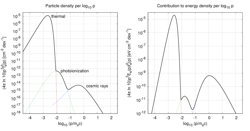
Figure 6: The phase space density of electrons at $z=2$ in the mean-density IGM. We show the thermal (Maxwell-Boltzmann), photoionization (Eq. 31), and cosmic ray components. The left panel is stretched to show particles per logarithmic range in momentum, while the right panel is weighted by energy.

5.3 Effect on plasma waves and ultrarelativistic beam instabilities

The plasma instabilities that are proposed to be relevant for TeV pair beams are associated with the growth of electrostatic plasma waves. An unmagnetized can undergo electrostatic oscillations at a frequency of

$$\omega_{\rm p}=c\sqrt{4\pi r_{0}n_{e}}=139\chi^{1/2}z_{2}^{3/2}\Delta^{1/2}\,{\rm s}^{-1},$$ (33)

where $z_{2}\equiv(1+z)/3$ and $\chi$ is the ionization fraction (normalized to 1 for fully ionized H⁺ and He²⁺). In the cold limit, the dispersion relation is truly flat, $\omega=\omega_{\rm p}$, the phase velocity is $v_{\rm ph}=\omega_{\rm p}/k$, and the group velocity is zero. The deviation of the plasma from being perfectly cold has two major effects. First, there is a correction to the real part of the frequency, $\Re\omega(k)-\omega_{\rm p}$, although this is small for the waves with $v_{\rm ph}/c$ of order unity that are relevant here. Secondly, there is a correction to the imaginary part $\Im\omega(k)$, which results in plasma waves growing ($\Im\omega>0$) or decaying ($\Im\omega<0$). We start from the form given by Beloborodov & Demianski (1995), which is valid for small numbers of non-thermal particles, including in the relativistic regime, with some algebraic rearrangement:

$$\Im\omega(k)=\frac{\pi\omega_{\rm p}}{2n_{e}}\left(\frac{m_{e}\omega_{\rm p}}{k}\right)^{2}\int_{{\mathbb{R}}^{3}}d^{3}{\bf p}\,\,\delta\left(m_{e}\omega_{\rm p}-\frac{{\bf k}\cdot{\bf p}}{\gamma}\right)\,{\bf k}\cdot\nabla_{\bf p}f_{e}({\bf p}),$$ (34)

where ${\bf p}$ is the electron momentum and $f_{e}({\bf p})$ is the phase space density. This correction is often negative (Landau damping), but can be positive if a beam is passing through the plasma (see Bret et al. 2010b for a review). For a narrow ultrarelativistic relativistic beam, $p\approx m_{e}c\gamma$, and the resonance condition in the $\delta$-function implies that modes with

$$k\approx\frac{\omega_{\rm p}}{c}\sec\theta$$ (35)

will be most strongly affected by the beam, where $\theta$ is the angle between ${\bf k}$ and the beam direction (see Bret et al. 2010a; Chang et al. 2016 for some fully worked examples).

If we take the isotropic population of $\sim\,$MeV cosmic rays to be isotropic, we may solve the problem in spherical polar coordinates, with $\tilde{\mu}$ as the cosine of the angle between ${\bf p}$ and ${\bf k}$: $d^{3}{\bf p}\rightarrow 2\pi p^{2}\,dp\,d\tilde{\mu}$. Then the $\tilde{\mu}$ integral is collapsed by the $\delta$ function at $\tilde{\mu}=\omega_{\rm p}/(kv)$ and we have a contribution to the growth rate:

$$\Im\omega = \frac{\pi^{2}\omega_{\rm p}}{n_{e}}\left(\frac{m_{e}\omega_{\rm p}}{k}\right)^{2}\int_{0}^{\infty}p^{2}\,dp\int_{-1}^{1}d\tilde{\mu}\,\delta(m_{e}(\omega_{\rm p}-kv\tilde{\mu}))\,k\tilde{\mu}\frac{df_{e}(p)}{dp}=\pi^{2}\omega_{\rm p}\left(\frac{m_{e}\omega_{\rm p}}{k}\right)^{3}\int_{p_{\rm min}}^{\infty}dp\,\left[1+\frac{p^{2}}{(m_{e}c)^{2}}\right]\frac{df_{e}(p)}{dp}$$ (36)

$$= -\frac{\pi^{2}\omega_{\rm p}}{n_{e}}\left(\frac{m_{e}\omega_{\rm p}}{k}\right)^{3}\left\{\left[1+\frac{p_{\rm min}^{2}}{(m_{e}c)^{2}}\right]f_{e}(p_{\rm min})+\frac{2}{(m_{e}c)^{2}}\int_{p_{\rm min}}^{\infty}pf_{e}(p)\,dp\right\},$$

where $v=p/\sqrt{p^{2}+(m_{e}c)^{2}}$ is the particle velocity; the minimum momentum of particles that can resonate with the wave is $p_{\rm min}=m_{e}v_{\rm min}/\sqrt{1-v_{\rm min}^{2}/c^{2}}$ and $v_{\rm min}=\omega_{\rm p}/k$; and in the last line we have integrated by parts. The resonance condition of course implies that $\Im\omega=0$ if $k<\omega_{\rm p}/c$. If we substitute the phase space density for $N(E)$ given by Eq. (32), and putting in the appropriate restriction on the range of $k$ using the Heaviside $\Theta$-function, Eq. (36) simplifies to

$$\Im\omega=-\frac{\pi}{4}\omega_{\rm p}\left(\frac{\omega_{\rm p}}{ck}\right)^{3}\frac{m_{e}c^{2}}{n_{e,\rm th}}\left\{\frac{E_{\rm min}+m_{e}c^{2}}{\sqrt{E_{\rm min}(E_{\rm min}+2m_{e}c^{2})}}N(E_{\rm min})+2\int_{E_{\rm min}}^{\infty}\frac{N(E)\,dE}{\sqrt{E(E+2m_{e}c^{2})}}\right\}\Theta\left(\frac{ck}{\omega_{\rm p}}-1\right)$$ (37)

with $E_{\rm min}=m_{e}c^{2}[(1-\omega_{\rm p}^{2}/c^{2}k^{2})^{-1/2}-1]$ being the kinetic energy of an electron whose velocity matches the phase velocity of the wave. The $-$ sign indicates that the plasma oscillations are damped. This reduces to the usual non-relativistic expression for Landau damping (Jackson, 1960) when $E\ll m_{e}c^{2}$; in this case only the first term in braces is significant.

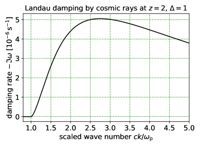
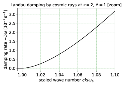
Figure 7: The linear Landau damping rate for plasma oscillations at $z=2$ and $\Delta=1$. The wavenumber is scaled by $\omega_{\rm p}/c=4.6\times 10^{-9}\,$cm^-1. Note that there is no linear Landau damping for phase velocities exceeding $c$ or $k<\omega_{\rm p}/c$.

The linear Landau damping rate caused by the $\sim$MeV cosmic rays is plotted in Fig. 7 for mean density at $z=2$, and for $1.2<ck/\omega_{\rm p}\lesssim 5$ it is a few$\times 10^{-6}\,$s^-1. For comparison, the instability growth rate $\Gamma_{\rm M,k}$ predicted by Broderick et al. (2012) is $\approx 2.7\times 10^{-11}E_{\rm TeV}^{3/2}\Delta^{-1/4}$ s^-1 for their fiducial blazar ($EL_{E}=10^{45}$ erg s^-1) at $z=2$ and at a distance of 1 pair production path length from the blazar; and the electron-ion collision rate is

$$\tau^{-1}_{ei}=\sqrt{\frac{32\pi}{9}}\,Zn_{e}r_{0}^{2}c^{4}\left(\frac{k_{\rm B}T}{m_{e}}\right)^{-3/2}\ln\Lambda=7.2\times 10^{-10}z_{2}^{3}\Delta T_{4}^{-3/2}\left(\frac{\ln\Lambda}{29.2}\right)~{}{\rm s}^{-1}$$ (38)

(e.g. Braginskii, 1965, Eq. 2.5e), where $Z$ is the weighted mean charge of the ions (1.14 after helium reionization), $T_{4}$ is the IGM temperature in units of $10^{4}$ K, and $\ln\Lambda$ is the Coulomb logarithm. It is readily seen that for $k\sim$few$\times\omega_{\rm p}/c$, the linear Landau damping operates at least thousands of times faster than either the pair beam instability or collisional effects. We thus conclude that in this range of wavenumbers, the oblique instability is simply shut off. The linear Landau damping rate is so enormous that even order-of-magnitude revisions in the MeV gamma ray background or the redshift dependence of its emissivity would not change the conclusion.

However, the resonance condition in Eq. (35) does allow a way out: at small angles, $ck/\omega_{\rm p}=1+\frac{1}{2}\theta^{2}+...$, the damping rate declines dramatically as $ck/\omega_{\rm p}\rightarrow 1$ (see the right-hand panel of Fig. 7). The essential reason is that plasma modes with small $\theta$ can resonate with the ultra-relativistic $\sim$TeV leptons in the pair beam ($v_{\rm ph}\approx c\cos\theta$), but can outrun the quasi-relativistic cosmic ray electrons, $v_{\rm ph}>c\beta$. Whether these very small-$\theta$ modes enable the plasma instabilities to proceed, and lead to dramatic angular broadening or partial thermalization of the beam energy, will be explored in future work.

5.4 Order-of-magnitude estimation of magnetic field generation

The cosmic rays considered in this paper should be considered as a potential source of magnetic fields. There are two classes of sources for magnetic fields in an initially unmagnetized plasma. The “battery” mechanisms deterministically generate a large-scale ${\boldsymbol{B}}$-field from inhomogeneities in a multi-component plasma. In “instability” mechanisms, the free energy in an anisotropic particle distribution can drive an instability on small scales (seeded by Poisson fluctuations if nothing else is available), resulting in a stochastic ${\boldsymbol{B}}$-field that grows exponentially until non-linear effects cause saturation. The classic examples of these mechanisms are the Biermann battery in an electron-ion plasma with misaligned temperature and density gradients (Biermann, 1950), and the Weibel instability in a plasma with quadrupolar anisotropy of the electron velocity distribution (Weibel, 1959).

We consider the magnetic field in the IGM generated by the electron cosmic rays via the return current battery mechanism (Ohira, 2020). The mechanism works slightly differently in the case that the thermal component is collisional on the cosmic ray transport timescale, as in the case of the IGM (Miniati & Bell, 2011). The key is that there will be a return current $-{\boldsymbol{J}}_{\rm CR}$ in the thermal medium, which implies an electric field ${\boldsymbol{E}}=\sigma_{\rm cond}^{-1}{\boldsymbol{J}}$ by Ohm’s law. Faraday’s law then implies that the curl component of this electric field is associated with a time-dependent magnetic field:

$$\frac{\partial{\boldsymbol{B}}}{\partial t}=c\,{\boldsymbol{\nabla}}\times(\sigma^{-1}_{\rm cond}{\boldsymbol{J}}_{\rm CR}),$$ (39)

where $\sigma_{\rm cond}$ is the conductivity of IGM and ${\boldsymbol{J}}_{\rm CR}=-e\,n_{\rm CR}{\boldsymbol{v}}_{\rm CR,bulk}$ is the electron cosmic ray current density.

Assuming the cosmic ray can diffuse in the Universe, we have the approximation $(v_{\rm bulk}\Delta t)/L\sim\mathcal{O}(1)$, where $L$ is the characteristic scale that matter density varies; this would be of order the filtering or the Jeans scale in the IGM. We also expect that when density perturbations are of order unity or greater, there is (at order of magnitude level) no special preference for the rotational vs. irrotational components of $\sigma^{-1}_{\rm cond}{\boldsymbol{J}}_{\rm CR}$. Therefore, we have

$$B\sim\frac{c\,e\,n_{\rm CR}}{\sigma_{\rm cond}}.$$ (40)

If the plasma is initially unmagnetized, we take the Spitzer conductivity (Spitzer & Härm, 1953):

$$\sigma_{\rm cond}=\frac{3}{4\sqrt{2\pi}}\frac{(k_{\rm B}T)^{3/2}}{Ze^{2}m_{\rm e}^{1/2}\ln{\Lambda}}\frac{1}{F(Z)},$$ (41)

where $k_{\rm B}$ is Boltzmann constant, $\ln{\Lambda}\sim 14$ is the Coulomb logarithm, for electron-hydrogen collision $Z=1$ and $F(Z)\sim 1/1.96$. Plugging into Eq. (40) the profiles of IGM temperature, number densities of cosmic rays we have in Sec. 5, we estimate the magnetic field as a function of redshift, shown in Fig. 8. The results show that the order of magnitude of this magnetic field is $\sim 10^{-25}$ G at $z\lesssim 4$. This is too small to have an impact on any known observable — indeed, the implied cyclotron frequency is approximately the Hubble rate. It is also small compared to the proposed field generation mechanisms from cosmic rays from early galaxies (Miniati & Bell, 2011), although the latter requires the cosmic rays to be able to freestream into the IGM without being confined by instabilities. So we do not expect the return current battery driven by the Compton-sourced electron cosmic rays to be significant.

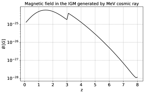
Figure 8: An order-of-magnitude estimate of the magnetic fields in the IGM generated by electron cosmic rays via the return current battery mechanism.

An alternative is to consider the quadrupole or Weibel (1959)-type instability mechanisms, which operate on an initially unmagnetized plasma. In the collisionless case, there is an instability for any non-zero quadrupole anisotropy in the particle momentum distribution, even when relativistic effects are considered (Lerche, 1969). We defer a full analysis for future work and focus here only on the orders of magnitude. As such, we will use the non-relativistic formulation, as described in Kahn (1962, 1964). If there is a cosmic ray component with number density $n_{e,\rm CR}$ and fractional quadrupole anisotropy $A_{\rm CR}$, and a thermal electron component with density $n_{e,\rm th}\gg n_{e,\rm CR}$, then the characteristic wavenumber $k_{\star}$ of the Weibel instability and its growth rate $\Gamma_{\star}$ are of order

$$k_{\star}\sim\left(A_{\rm CR}\frac{n_{e,\rm CR}}{n_{e,\rm th}}\right)^{1/2}\frac{\omega_{\rm p}}{c}~{}~{}~{}{\rm and}~{}~{}~{}\Gamma_{\star}\sim\left(A_{\rm CR}\frac{n_{e,\rm CR}}{n_{e,\rm th}}\right)^{3/2}\frac{v_{e,\rm th}}{c}\omega_{\rm p},$$ (42)

where $v_{e,\rm th}$ is the electron thermal velocity. At $z\sim 2$, we estimate the growth rate to be $\sim 10^{-15}A_{\rm CR}^{3/2}\,$s^-1. It is not clear what quadrupole anisotropy to expect for the cosmic rays, and it presumably depends on where one is between the diffusion and free-streaming limits. However, even a few percent-level anisotropy is not sufficient to drive the Weibel instability in less than a Hubble time, and regardless of $A_{\rm CR}$ the timescales are long enough for collisions to be relevant. We therefore expect that the Weibel instability driven by Compton-induced cosmic ray electrons is not likely to be operative.

6 Discussion

We have shown in this paper that cosmic ray electrons are ubiquitous in the IGM. They contribute about 0.3% to thermal pressure in the IGM at $z$ = 2 at mean density, rising to 1.0% at $z$ = 1 and 1.8% at $z$ = 0.1. Our study also reveals that cosmic ray electrons induce linear Landau damping of plasma oscillations at a rate significantly faster than previously predicted instability and collision rates. This damping effectively suppresses the oblique instability of TeV pair beams in the IGM over most of the relevant phase space. Oblique instability modes with very small angle $\theta$ relative to the TeV pair beam survive because the linear Landau damping by the cosmic ray background is driven by particles with velocity $v\geq c\cos\theta$, or equivalently Lorentz factors $\gamma>1/\sin\theta$.

Our findings are subject to model uncertainties, but by far the largest is the gamma ray background model. In this paper, we adopt the model in Khaire & Srianand (2019) as our foundational EBL source model. The fractional contribution of cosmic ray electrons to the IGM pressure at mean density using the alternative Haardt & Madau (2012) model is 0.5% at $z=0.1$, 0.22% at $z=1$, and 0.05% at $z=2$; this is a factor of 3.6, 4.5, and 6 lower than in the Khaire & Srianand (2019) model, respectively. The Haardt & Madau (2012) model was intended primarily for ultraviolet/X-ray applications, and it exhibits an exponential cutoff in the energy distribution for Type 2 AGN instead of matching observed $\geq$MeV gamma ray background. The Khaire & Srianand (2019) model, on the other hand, extends the Type 2 AGN spectrum into the MeV region and normalizes it to match the observed background. This is not the only possible source for the gamma-ray background, but as long as the source invoked to explain it exhibits cosmological evolution reasonably similar to star formation or AGN activity, the specific model choice becomes less critical for estimating a background model. Therefore, we believe the use of the Khaire & Srianand (2019) model as our fiducial model is appropriate. However, the linear Landau damping rate is so enormous that even order-of magnitude revisions in the MeV gamma ray background or the redshift dependence of its emissivity would not change the conclusion.

The presence of cosmic ray electrons everywhere in the IGM has several other potential implications. One is on the Lyman-$\alpha$ forest, where extremely high precision measurements are now possible and the interpretation might be affected by the small non-thermal contributions to the pressure discussed in this work. For example, the extended Baryon Oscillation Spectroscopic Survey (eBOSS) has measured the amplitude of fluctuations $\sigma_{8}$ to $\pm 2.6\%$ (Chabanier et al., 2019); the ongoing Dark Energy Spectroscopic Instrument (DESI) survey aims to measure the slope of the spectral index $n_{s}$ to $\pm 0.0029$ via the Lyman-$\alpha$ forest (DESI Collaboration et al., 2016), and future surveys with many more sightlines are being proposed (Schlegel et al., 2022). A new contribution to IGM pressure at the percent level might therefore be significant for the future experiments. On the other hand, there are likely some (partial) degeneracies between the non-thermal pressure and other IGM thermodynamics parameters that are already marginalized in Lyman-$\alpha$ forest analyses, and cosmological parameters such as $\sigma_{8}$ and $n_{s}$ can sometimes be constrained quite well even when there are degeneracies in the IGM thermodynamics parameters (Chabanier et al., 2019). It also “helps” that the cosmic ray electron contribution increases toward lower redshift, whereas ground-based Lyman-$\alpha$ forest observations are restricted to $z\gtrsim 1.7$ by atmospheric opacity.

Another possible implication is that cosmic rays are implicated in several of the proposed mechanisms for generating magnetic fields in the IGM directly via battery mechanisms (Ohira, 2020) or via instabilities driven by cosmic ray anisotropy, such as the dipole-driven non-resonant streaming instability, which can grow from a very small but non-zero background field (Bell, 2004); and the quadrupole-driven Weibel-type instabilities, which in the collisionless limit can grow starting from no background magnetic field and an arbitrarily small anisotropy (Weibel, 1959), even in the relativistic regime (Lerche, 1969). We have investigated these mechanisms and found them to be likely insufficient for magnetic field generation in the IGM: the order of magnitude of magnetic fields generated via battery mechanisms are estimated to be up to $\sim 10^{-25}$ G, and the timescale for the cosmic ray anisotropy-driven Weibel instability is too long.

In conclusion, although much work remains to understand the implications, it is evident that the cosmic ray electron population is an important ingredient in the evolution of the TeV pair beams from blazars, and more generally in the plasma physics of the intergalactic medium.

References

- Acero et al. (2016) Acero, F., Ackermann, M., Ajello, M., et al. 2016, ApJS, 223, 26, doi: 10.3847/0067-0049/223/2/26
- Ackermann et al. (2012) Ackermann, M., Ajello, M., Atwood, W. B., et al. 2012, ApJ, 750, 3, doi: 10.1088/0004-637X/750/1/3
- Adriani et al. (2011) Adriani, O., Barbarino, G. C., Bazilevskaya, G. A., et al. 2011, Phys. Rev. Lett., 106, 201101, doi: 10.1103/PhysRevLett.106.201101
- Aguilar et al. (2019) Aguilar, M., Ali Cavasonza, L., Alpat, B., et al. 2019, Phys. Rev. Lett., 122, 101101, doi: 10.1103/PhysRevLett.122.101101
- Amano & Hoshino (2010) Amano, T., & Hoshino, M. 2010, Phys. Rev. Lett., 104, 181102, doi: 10.1103/PhysRevLett.104.181102
- Axford et al. (1977) Axford, W. I., Leer, E., & Skadron, G. 1977, in International Cosmic Ray Conference, Vol. 11, International Cosmic Ray Conference, 132
- Bell (1978) Bell, A. R. 1978, MNRAS, 182, 147, doi: 10.1093/mnras/182.2.147
- Bell (2004) —. 2004, MNRAS, 353, 550, doi: 10.1111/j.1365-2966.2004.08097.x
- Beloborodov & Demianski (1995) Beloborodov, A. M., & Demianski, M. 1995, Phys. Rev. Lett., 74, 2232, doi: 10.1103/PhysRevLett.74.2232
- Berger & Seltzer (1982) Berger, M. J., & Seltzer, S. M. 1982, Stopping powers and ranges of electrons and positrons
- Bethe & Salpeter (1957) Bethe, H. A., & Salpeter, E. E. 1957, Quantum Mechanics of One- and Two-Electron Atoms
- Biermann (1950) Biermann, L. 1950, Zeitschrift Naturforschung Teil A, 5, 65
- Blanco et al. (2023) Blanco, C., Ghosh, O., Jacobsen, S., & Linden, T. 2023, arXiv e-prints, arXiv:2303.01524, doi: 10.48550/arXiv.2303.01524
- Blandford & Ostriker (1978) Blandford, R. D., & Ostriker, J. P. 1978, ApJ, 221, L29, doi: 10.1086/182658
- Boezio et al. (2000) Boezio, M., Carlson, P., Francke, T., et al. 2000, ApJ, 532, 653, doi: 10.1086/308545
- Böss et al. (2023) Böss, L. M., Steinwandel, U. P., Dolag, K., & Lesch, H. 2023, MNRAS, 519, 548, doi: 10.1093/mnras/stac3584
- Braginskii (1965) Braginskii, S. I. 1965, Reviews of Plasma Physics, 1, 205
- Bret et al. (2010a) Bret, A., Gremillet, L., & Bénisti, D. 2010a, Phys. Rev. E, 81, 036402, doi: 10.1103/PhysRevE.81.036402
- Bret et al. (2010b) Bret, A., Gremillet, L., & Dieckmann, M. E. 2010b, Physics of Plasmas, 17, 120501, doi: 10.1063/1.3514586
- Broderick et al. (2012) Broderick, A. E., Chang, P., & Pfrommer, C. 2012, ApJ, 752, 22, doi: 10.1088/0004-637X/752/1/22
- Chabanier et al. (2019) Chabanier, S., Palanque-Delabrouille, N., Yèche, C., et al. 2019, J. Cosmology Astropart. Phys, 2019, 017, doi: 10.1088/1475-7516/2019/07/017
- Chang et al. (2012) Chang, P., Broderick, A. E., & Pfrommer, C. 2012, ApJ, 752, 23, doi: 10.1088/0004-637X/752/1/23
- Chang et al. (2014) Chang, P., Broderick, A. E., Pfrommer, C., et al. 2014, ApJ, 797, 110, doi: 10.1088/0004-637X/797/2/110
- Chang et al. (2016) —. 2016, ApJ, 833, 118, doi: 10.3847/1538-4357/833/1/118
- Cummings et al. (2016) Cummings, A. C., Stone, E. C., Heikkila, B. C., et al. 2016, ApJ, 831, 18, doi: 10.3847/0004-637X/831/1/18
- DESI Collaboration et al. (2016) DESI Collaboration, Aghamousa, A., Aguilar, J., et al. 2016, arXiv e-prints, arXiv:1611.00036, doi: 10.48550/arXiv.1611.00036
- Draine (2011) Draine, B. T. 2011, Physics of the Interstellar and Intergalactic Medium
- Fano (1956) Fano, U. 1956, Physical Review, 103, 1202, doi: 10.1103/PhysRev.103.1202
- Fano (1963) —. 1963, Annual Review of Nuclear and Particle Science, 13, 1, doi: 10.1146/annurev.ns.13.120163.000245
- Feretti et al. (2012) Feretti, L., Giovannini, G., Govoni, F., & Murgia, M. 2012, A&A Rev., 20, 54, doi: 10.1007/s00159-012-0054-z
- Ferrari et al. (2008) Ferrari, C., Govoni, F., Schindler, S., Bykov, A. M., & Rephaeli, Y. 2008, Space Sci. Rev., 134, 93, doi: 10.1007/s11214-008-9311-x
- Ha et al. (2018) Ha, J.-H., Ryu, D., Kang, H., & van Marle, A. J. 2018, ApJ, 864, 105, doi: 10.3847/1538-4357/aad634
- Haardt & Madau (2012) Haardt, F., & Madau, P. 2012, ApJ, 746, 125, doi: 10.1088/0004-637X/746/2/125
- Harris et al. (2020) Harris, C. R., Millman, K. J., van der Walt, S. J., et al. 2020, Nature, 585, 357, doi: 10.1038/s41586-020-2649-2
- Hirata (2018) Hirata, C. M. 2018, MNRAS, 474, 2173, doi: 10.1093/mnras/stx2854
- Hui & Gnedin (1997) Hui, L., & Gnedin, N. Y. 1997, MNRAS, 292, 27, doi: 10.1093/mnras/292.1.27
- Hunter (2007) Hunter, J. D. 2007, Computing in Science & Engineering, 9, 90, doi: 10.1109/MCSE.2007.55
- Iwabuchi & Kumagai (2001) Iwabuchi, K., & Kumagai, S. 2001, PASJ, 53, 669, doi: 10.1093/pasj/53.4.669
- Jackson (1960) Jackson, J. D. 1960, Journal of Nuclear Energy, 1, 171, doi: 10.1088/0368-3281/1/4/301
- Jones (1965) Jones, F. C. 1965, Physical Review, 137, 1306, doi: 10.1103/PhysRev.137.B1306
- Kahn (1962) Kahn, F. D. 1962, Journal of Fluid Mechanics, 14, 321, doi: 10.1017/S0022112062001275
- Kahn (1964) —. 1964, Journal of Fluid Mechanics, 19, 210, doi: 10.1017/S0022112064000660
- Khaire & Srianand (2019) Khaire, V., & Srianand, R. 2019, MNRAS, 484, 4174, doi: 10.1093/mnras/stz174
- Kobzar et al. (2021) Kobzar, O., Niemiec, J., Amano, T., et al. 2021, ApJ, 919, 97, doi: 10.3847/1538-4357/ac1107
- Lacki (2015) Lacki, B. C. 2015, MNRAS, 448, L20, doi: 10.1093/mnrasl/slu186
- Lacki et al. (2014) Lacki, B. C., Horiuchi, S., & Beacom, J. F. 2014, ApJ, 786, 40, doi: 10.1088/0004-637X/786/1/40
- Lerche (1969) Lerche, I. 1969, Journal of Mathematical Physics, 10, 13, doi: 10.1063/1.1664748
- Madau & Efstathiou (1999) Madau, P., & Efstathiou, G. 1999, ApJ, 517, L9, doi: 10.1086/312022
- Miniati & Bell (2011) Miniati, F., & Bell, A. R. 2011, ApJ, 729, 73, doi: 10.1088/0004-637X/729/1/73
- Miniati & Elyiv (2013) Miniati, F., & Elyiv, A. 2013, ApJ, 770, 54, doi: 10.1088/0004-637X/770/1/54
- Møller (1932) Møller, C. 1932, Annalen der Physik, 406, 531, doi: 10.1002/andp.19324060506
- Ohira (2020) Ohira, Y. 2020, ApJ, 896, L12, doi: 10.3847/2041-8213/ab963d
- Orlando et al. (2018) Orlando, E., Johannesson, G., Moskalenko, I. V., Porter, T. A., & Strong, A. 2018, Nuclear and Particle Physics Proceedings, 297-299, 129, doi: 10.1016/j.nuclphysbps.2018.07.020
- Orlando & Strong (2013) Orlando, E., & Strong, A. 2013, MNRAS, 436, 2127, doi: 10.1093/mnras/stt1718
- Peebles (1967) Peebles, P. J. E. 1967, ApJ, 147, 859, doi: 10.1086/149077
- Pequignot et al. (1991) Pequignot, D., Petitjean, P., & Boisson, C. 1991, A&A, 251, 680
- Pfrommer et al. (2017) Pfrommer, C., Pakmor, R., Schaal, K., Simpson, C. M., & Springel, V. 2017, MNRAS, 465, 4500, doi: 10.1093/mnras/stw2941
- Planck Collaboration et al. (2020) Planck Collaboration, Aghanim, N., Akrami, Y., et al. 2020, A&A, 641, A6, doi: 10.1051/0004-6361/201833910
- Riquelme & Spitkovsky (2011) Riquelme, M. A., & Spitkovsky, A. 2011, ApJ, 733, 63, doi: 10.1088/0004-637X/733/1/63
- Rohrlich & Carlson (1954) Rohrlich, F., & Carlson, B. C. 1954, Physical Review, 93, 38, doi: 10.1103/PhysRev.93.38
- Sauer et al. (2014) Sauer, S. P. A., Haq, I. U., Sabin, J. R., et al. 2014, Molecular Physics, 112, 751, doi: 10.1080/00268976.2013.858192
- Schlegel et al. (2022) Schlegel, D. J., Kollmeier, J. A., Aldering, G., et al. 2022, arXiv e-prints, arXiv:2209.04322, doi: 10.48550/arXiv.2209.04322
- Schlickeiser et al. (2013) Schlickeiser, R., Krakau, S., & Supsar, M. 2013, ApJ, 777, 49, doi: 10.1088/0004-637X/777/1/49
- Shalaby et al. (2018) Shalaby, M., Broderick, A. E., Chang, P., et al. 2018, ApJ, 859, 45, doi: 10.3847/1538-4357/aabe92
- Shalaby et al. (2022) Shalaby, M., Lemmerz, R., Thomas, T., & Pfrommer, C. 2022, ApJ, 932, 86, doi: 10.3847/1538-4357/ac6ce7
- Shapiro et al. (2004) Shapiro, P. R., Iliev, I. T., & Raga, A. C. 2004, MNRAS, 348, 753, doi: 10.1111/j.1365-2966.2004.07364.x
- Sironi & Giannios (2014) Sironi, L., & Giannios, D. 2014, ApJ, 787, 49, doi: 10.1088/0004-637X/787/1/49
- Spitzer & Härm (1953) Spitzer, L., & Härm, R. 1953, Physical Review, 89, 977, doi: 10.1103/PhysRev.89.977
- Stone et al. (2013) Stone, E. C., Cummings, A. C., McDonald, F. B., et al. 2013, Science, 341, 150, doi: 10.1126/science.1236408
- Strigari et al. (2005) Strigari, L. E., Beacom, J. F., Walker, T. P., & Zhang, P. 2005, J. Cosmology Astropart. Phys, 2005, 017, doi: 10.1088/1475-7516/2005/04/017
- Uehling (1954) Uehling, E. A. 1954, Annual Review of Nuclear and Particle Science, 4, 315, doi: 10.1146/annurev.ns.04.120154.001531
- Upton Sanderbeck et al. (2016) Upton Sanderbeck, P. R., D’Aloisio, A., & McQuinn, M. J. 2016, MNRAS, 460, 1885, doi: 10.1093/mnras/stw1117
- van Weeren et al. (2019) van Weeren, R. J., de Gasperin, F., Akamatsu, H., et al. 2019, Space Sci. Rev., 215, 16, doi: 10.1007/s11214-019-0584-z
- Watanabe et al. (2000) Watanabe, K., Leising, M. D., Share, G. H., & Kinzer, R. L. 2000, in American Institute of Physics Conference Series, Vol. 510, The Fifth Compton Symposium, ed. M. L. McConnell & J. M. Ryan, 471–475, doi: 10.1063/1.1303252
- Weibel (1959) Weibel, E. S. 1959, Phys. Rev. Lett., 2, 83, doi: 10.1103/PhysRevLett.2.83
- Weidenspointner et al. (2000) Weidenspointner, G., Varendorff, M., Kappadath, S. C., et al. 2000, in American Institute of Physics Conference Series, Vol. 510, The Fifth Compton Symposium, ed. M. L. McConnell & J. M. Ryan, 467–470, doi: 10.1063/1.1307028