Study of Charged Celestial Objects in Modified Gravity

Abstract

In this paper, we assess different charged self-gravitating stellar models possessing anisotropic matter source in the background of $f(G,T)$ gravity. For this purpose, we choose a well-known model of this gravity, i.e., $f(G,T)=G^{2}+\varrho T$, where $\varrho$ stands for the coupling constant. The modified field equations are developed using MIT bag model equation of state, and their solution is found with the help of Tolman IV ansatz which contains three unknown constants. This solution is further exploited to examine the graphical behavior of Her X-I, PSR J1614-2230, 4U1820-30 and LMC X-4 celestial objects. We assume two different values of charge to figure out the pressure constituents, energy density, anisotropy and energy constraints graphically. We also discuss compactness, mass and redshift parameters. Finally, we explore stability of the considered stars through two different methods. It is concluded that all the star candidates are viable as well as stable for $\mathcal{Q}=0.1$. For the larger charge, the viable behavior is also observed for all stars but PSR J1614-2230 shows unstable trend.

Keywords: Stellar structures; Exact solutions; $f(G,T)$ gravity; Anisotropy.
PACS: 04.50.Kd; 95.30.-k; 04.20.Jb; 04.40.Dg

1 Introduction

The eye-catching fundamental astrophysical objects, i.e., stars are present alongside other constituents in the cosmos. Astrophysicists got captivated by these objects and devoted their attention to studying the secrets behind their evolutionary processes. The existence of heat and luminosity in the cosmic world is the result of multiple nuclear reactions that occur in the middle of celestial bodies. In the meantime, there arises a stage in which the gravitational force (acting internally) becomes dominant over the outward-producing pressure. It leads to the collapse of astronomical bodies and the beginning of some new celestial entities, namely white dwarf, neutron star, and black hole. In order to stop further collapse in neutron stars, the neutrons produce degeneracy pressure, which operates in the opposite direction of gravity. The anticipation of neutron stars was predicted for the first time in 1934 [1], although their emergence was confirmed afterwards. A strange star is an extremely dense intermediate state that exists between neutron stars and black holes and includes quark matter. These stars are thought to have interiors made up of up, down, and strange quarks, which are far more massive than neutron stars. Many researchers made early attempts to comprehend these hypothetical systems [2].

The anisotropic matter distribution is assumed to be a good source of study to understand the interior composition and dynamics of stellar objects. Pressure anisotropy is caused by the discrepancy between radial and tangential pressures. Ruderman [3] suggested that anisotropy in the compact bodies with denser cores is generated due to the interacting nuclear matter. The physical attributes of anisotropic stellar structures are studied by Dev and Gleiser [4] using various equations of state (EoS) that relate tangential and radial pressure components. Hossein et al [5] investigated the key characteristics of 4U1820-30 through graphical interpretation by including the cosmological constant in the field equations. Kalam et al [6] checked the viability and stability of numerous neutron stars. The embedding class 1 solution is used to derive the anisotropic results through which the physical acceptance conditions of stars are checked by Maurya et al [7]. The inclusion of electric charge in the inner distribution provides a comprehensive way to apprehend the expansion and stability of celestial structures. Charges produce a force in the outward direction that acts against gravity and supports the objects in sustaining their existence for a longer time. Murad [8] assumed the anisotropic effects on charged stellar bodies to derive their solution and visualized them graphically. The condition of conformal symmetry has been utilized in extracting the effects of electromagnetic field on realistic models by Matondo et al [9]. A significant work to realize the contribution of electric charge on different structures has been accomplished in [10].

The MIT bag model EoS is found more useful in describing the interior structure of quark objects. It is important to mention here that the compactness of the astronomical stars 4U 1820-30, SAX J 1808.4-3658, Her X-1, 4U 1728-34, PSR 0943+10, RXJ 185635- 3754 was not proficiently measured through neutron star EoS, whereas more considerable results have been produced with quark matter EoS [11]. The difference between real and false vacuums can be evaluated with the help of bag constant present in the bag model EoS. It is observed that the increment in the values of $\mathfrak{B}_{c}$ decreases the quark pressure. For the exploration of inner configuration of quark stars associated with MIT bag EoS, there is a large body of literature. When Demorest et al [12] observed the candidate PSR J1614-2230, they found that these kinds of massive bodies can be elucidated more efficiently through MIT bag EoS. Using the interpolation method, Rahaman et al. [13] determined the mass of quark star with a radius of 9.9 km and used this finding to explain several physical aspects. Bhar [14] explored certain compact entities experiencing anisotropy in the light of Krori-Barua ansatz and MIT bag EoS. Using corresponding EoS, Deb et al [15] examined the essential constraints to be fulfilled for physically acceptable stars in the case of charged/uncharged sources. Sharif and his collaborators [16] developed non-singular solution of the field equations to analyze the anisotropic stellar systems.

The general theory of relativity (GR) is taken into account as a foundation to comprehend the gravitational interaction at large scales. This has played a crucial role in opening new windows to the discovery of mysterious entities. The existence of dark energy, which has large negative pressure and is thought to be the primary source of cosmic development, as well as dark matter, are two main issues that GR does not adequately address. Thus, an attempt to uncover these mysterious components is achieved by altering the Einstein-Hilbert action that gives rise to the formulation of modified gravity.

In this respect, the Ricci scalar $R$ in the Einstein-Hilbert action is interchanged from its generalized function to yield the first modified theory namely, $f(R)$ gravity. Various researchers have inspected inflationary and current cosmic acceleration in the realm of feasible $f(R)$ models [17]. Also, a large number of stellar bodies possessing fundamental characteristics have been discussed by employing different methods in this theory [18]. A wide range of modified theories with arbitrary coupling are of great interest to astrophysicists. In order to obtain the exciting results, Harko et al [19] coupled geometry with matter in the action and proposed $f(R,T)$ gravity, where $T$ indicates the trace of energy-momentum tensor. The impact of minimal/non-minimal interactions on test particles has been analyzed using several $f(R,T)$ models. Numerous researchers have examined various configurations and noticed fascinating astrophysical findings in this theory [20].

In addition to the aforementioned theories, $f(G)$ gravity is another modification of GR which is formulated by Nojiri and Odintsov [21] by adding $f(G)$ ($G$ is the Gauss-Bonnet invariant (GB)) with $R$. Moreover, the expression of GB is specified as $G=R^{\phi\sigma\gamma\delta}R_{\phi\sigma\gamma\delta}+R^{2}-4R^{\phi\sigma}R_{\phi\sigma}$, with $R_{\phi\sigma}$ and $R_{\phi\sigma\gamma\delta}$ being the Ricci and Riemann tensors, respectively. Four different kinds of future singularities were investigated under the reconstruction of feasible $f(G)$ model by Bamba et al [22] corresponding to the phantom or quintessence accelerating epoch. In modified Gauss-Bonnet gravity, Myrzakulov et al [23] established the cosmic solutions without including cosmological constant and effectively described the existence of dark energy and inflationary epoch. The analysis of accelerating expansion with viable $f(G)$ model is executed by computing the symmetry generators according to the separation of variables and power-law type (employing Noether symmetry approach) [24]. The values of Hubble, jerk, snap and deceleration parameters have been kept fixed by Bamba et al [25] in order to look for the regular configured source by utilizing three $f(G)$ ansatzs. Sharif and Ramzan [26] used the radii and masses of several astronomical bodies to observe their viable and stable characters under the influence of modified Guass-Bonnet theory.

Sharif and Ikram [27] got inspired from the geometry-matter coupling and developed another novel theory by substituting the function $f(G,T)$ in place of $f(G)$ and naming it $f(G,T)$ gravity. Shamir and Ahmad [28] focused on exploring the physical attributes of three stellar entities undergoing anisotropy in the framework of $f(G,T)$ gravity. The compact star Vela X-1 was chosen by Maurya et al [29] to estimate the viable and stable features of its inner anisotropic source. Sharif and Naeem [30] discussed the novel characteristics of static anisotropic fluid spheres in this theory. Recently, we have calculated the $Y_{TF}$ factor to observe the complex structures by employing Herrera’s decomposing technique for static charged and uncharged sources, non-static cylindrical and spherical (charged/uncharged) systems [31].

In this paper, we focus on revealing the contribution of electromagnetic field and $f(G,T)$ gravity in studying the physical aspects of quark candidates. The paper is structured as follows. In section 2, primitive idea of this gravity, crucial equations and Tolman IV solution are examined. Section 3 uses the boundary conditions to generally express the constants (in Tolman IV) in the observational data of stars. The physical acceptance and key features of all compact objects corresponding to two charge values are reviewed in section 4. The last section describes the significant outcomes.

2 $f(G,T)$ Gravity and Matter Determinants

The action of $f(G,T)$ gravity together with Ricci scalar in the Einstein-Maxwell action is given as follows

$$\mathfrak{I}_{f(G,T)}=\frac{1}{16\pi}\int\big{(}f(G,T)+R\big{)}d^{4}x\sqrt{-g}+\int\big{(}\mathfrak{L}_{\mathbf{E}}+\mathfrak{L}_{\mathbf{M}})d^{4}x\sqrt{-g},$$ (1)

where $\mathfrak{L}_{\mathbf{E}}$ specifies the Lagrangian density associated with the electromagnetic field and for the usual matter distribution it is denoted by $\mathfrak{L}_{\mathbf{M}}$. The symbol $g$ indicates determinant of the metric tensor and the Lagrangian density for the present setup is fixed as $\mathfrak{L}_{\mathbf{M}}=\mathbb{P}$. The relation between the energy-momentum tensor and Lagrangian density is observed as

$$T_{\phi\sigma}=g_{\phi\sigma}\mathfrak{L}_{\mathbf{M}}-\frac{2\partial\mathfrak{L}_{\mathbf{M}}}{\partial g^{\phi\sigma}}.$$ (2)

In the present system, the action (1) is varied with $g_{\phi\sigma}$ to develop the field equations which are given as follows

$$G_{\phi\sigma} = 8\pi(T^{(\textsf{m})}_{\phi\sigma}+\mathcal{S}_{\phi\sigma})-(T^{(\textsf{m})}_{\phi\sigma}+\Theta_{\phi\sigma})f_{T}(G,T)+\frac{1}{2}g_{\phi\sigma}f(G,T)+\big{(}4R^{\mu\nu}R_{\phi\mu\sigma\nu}$$ (3)

$$- 2RR_{\phi\sigma}-2R^{\mu\nu\gamma}_{\phi}R_{\sigma\mu\nu\gamma}+4R_{\mu\sigma}R^{\mu}_{\phi}\big{)}f_{G}(G,T)+(4g_{\phi\sigma}R^{\mu\nu}\nabla_{\mu}\nabla_{\nu}$$

$$- 4R^{\mu}_{\phi}\nabla_{\sigma}\nabla_{\mu}-4R_{\phi\mu\sigma\nu}\nabla^{\mu}\nabla^{\nu}-2g_{\phi\sigma}R\nabla^{2}+2R\nabla_{\phi}\nabla_{\sigma}-4R^{\mu}_{\sigma}\nabla_{\phi}\nabla_{\mu}$$

$$+ 4R_{\phi\sigma}\nabla^{2})f_{G}(G,T),$$

where $\Theta_{\phi\sigma}=-2T^{(\textsf{m})}_{\phi\sigma}+\mathbb{P}g_{\phi\sigma}$ along with $\mathbb{P}=\frac{\mathbb{P}_{r}+2\mathbb{P}_{t}}{3}$ and the geometrical representation of the celestial bodies is provided by the Einstein tensor ($G_{\phi\sigma}$). The expressions $f_{T}$ and $f_{G}$ are given as $\frac{\partial f(G,T)}{\partial T}$ and $\frac{\partial f(G,T)}{\partial G}$, respectively. Moreover, the term $\nabla_{\phi}$ is the covariant derivative and the d’ Alembert operator is signified by $\nabla^{2}=\nabla^{a}\nabla_{a}=\Box$. The replacement $f(G,T)=f(G)$ in the action produces the field equations of $f(G)$ theory. The contribution of extra terms in this theory is represented by

$$T^{\textsf{cor}}_{\phi\sigma} =\frac{1}{8\pi}\bigg{[}\{(\mathbb{U}+\mathbb{P}_{t})\textsf{W}_{\phi}\textsf{W}_{\sigma}-\frac{1}{3}(\mathbb{P}_{r}-\mathbb{P}_{t})g_{\phi\sigma}+(\mathbb{P}_{r}-\mathbb{P}_{t})\textsf{X}_{\phi}\textsf{X}_{\sigma}\}f_{T}(G,T)$$

$$+\frac{1}{2}g_{\phi\sigma}f(G,T)+\big{(}4R^{\mu\nu}R_{\phi\mu\sigma\nu}-2RR_{\phi\sigma}-2R^{\mu\nu\gamma}_{\phi}R_{\sigma\mu\nu\gamma}+4R_{\mu\sigma}R^{\mu}_{\phi}\big{)}f_{G}(G,T)$$

$$+(4g_{\phi\sigma}R^{\mu\nu}\nabla_{\mu}\nabla_{\nu}-4R^{\mu}_{\phi}\nabla_{\sigma}\nabla_{\mu}-4R_{\phi\mu\sigma\nu}\nabla^{\mu}\nabla^{\nu}-2g_{\phi\sigma}R\nabla^{2}+2R\nabla_{\phi}\nabla_{\sigma}$$

$$-4R^{\mu}_{\sigma}\nabla_{\phi}\nabla_{\mu}+4R_{\phi\sigma}\nabla^{2})f_{G}(G,T)\bigg{]}.$$ (4)

The following energy-momentum tensor is employed to examine the substantial features of anisotropic stellar candidates as

$$T^{(\textsf{m})}_{\phi\sigma}=(\mathbb{U}+\mathbb{P}_{t})\textsf{W}_{\phi}\textsf{W}_{\sigma}+\mathbb{P}_{t}g_{\phi\sigma}+(\mathbb{P}_{r}-\mathbb{P}_{t})\textsf{X}_{\phi}\textsf{X}_{\sigma},$$ (5)

where pressures in the radial and tangential directions are indicated by $\mathbb{P}_{r}$ and $\mathbb{P}_{t}$, respectively, and $\mathbb{U}$ stands for the energy density of the fluid source. The covariant component of four-vector is expressed as $\textsf{X}_{\phi}$ and of four-velocity is denoted by $\textsf{W}_{\phi}$, portraying the relations $\textsf{X}^{\phi}\textsf{W}_{\phi}=0$ and $\textsf{W}^{\phi}\textsf{W}_{\phi}=-1$. The alternative way of presenting Eq.(4) is

$$G_{\phi\sigma}=8\pi T^{\texttt{(tot)}}_{\phi\sigma}=8\pi(T^{\textsf{cor}}_{\phi\sigma}+T^{(\textsf{m})}_{\phi\sigma}).$$ (6)

The electromagnetic energy tensor to discuss the charged fluid within the compact bodies is characterized by

$$\mathcal{S}_{\phi\sigma}=\frac{1}{4\pi}\left(\mathcal{F}^{n}_{\phi}\mathcal{F}_{\sigma n}-\frac{1}{4}\mathcal{F}_{nm}\mathcal{F}^{nm}g_{\phi\sigma}\right),$$ (7)

where the Maxwell field tensor is specified as $\mathcal{F}_{\phi\sigma}=\xi_{\sigma,\phi}-\xi_{\phi,\sigma}$ and the four potential is represented by $\xi_{\phi}$. For the static symmetric structure, it takes the form $\xi_{\phi}=\xi(r)\delta^{0}_{\phi}$. The tensorial form of Maxwell field equations turn out to be

$$\mathcal{F}_{[\phi\sigma;n]}=0,\quad\mathcal{F}^{\phi\sigma}_{~{}~{};\sigma}=4\pi\mathcal{J}^{\phi},$$

where $\mathcal{J}^{\phi}$ indicates the electromagnetic four-current vector with $\mathcal{J}^{\phi}=\vartheta\textsf{W}^{\phi}$ and $\vartheta$ stands for the charge density. The energy-momentum tensor in this theory is non-conserved as a result of interaction between matter source and geometrical terms. It causes to generate an extra force due to which the massive particles are forced to stop their geodesic motion in the gravitational field. The equation corresponding to the non-zero divergence of fluid configuration is given by

$$\nabla^{\phi}T_{\phi\sigma} = \frac{f_{T}(G,T)}{8\pi-f_{T}(G,T)}\bigg{[}-\frac{1}{2}g_{\phi\sigma}\nabla^{\phi}T+(\Theta_{\phi\sigma}+T_{\phi\sigma})\nabla^{\phi}(\ln f_{T}(G,T))$$ (8)

$$+ \nabla^{\phi}\Theta_{\phi\sigma}\bigg{]}.$$

The geometrical structure under discussion is chosen to be a spherical symmetric distribution which is separated by a hypersurface ($\Sigma$) into two regions (i.e., outer and inner). The internal composition is discussed by using the metric as

$$ds^{2}=-e^{\eta}dt^{2}+e^{\delta}dr^{2}+r^{2}d\theta^{2}+r^{2}{\sin^{2}\theta}{d\phi^{2}},$$ (9)

where $\eta=\eta(r)$ and $\delta=\delta(r)$. The contravariant component of four-velocity and four-vector in terms of metric potentials are delineated as

$$\textsf{W}^{\phi}=\left(e^{\frac{-\eta}{2}},0,0,0\right),\quad\textsf{X}^{\phi}=\left(0,e^{\frac{-\delta}{2}},0,0\right).$$ (10)

The feasibility and stability of anisotropic compact entities are observed by utilizing a minimal $f(G,T)$ model [28, 30], prescribed as

$$f(G,T)=\mathfrak{t_{1}}(G)+\mathfrak{t_{2}}(T),$$ (11)

where it can be easily seen that $\mathfrak{t_{1}}$ and $\mathfrak{t_{2}}$ depend only on $G$ and $T$, respectively. The vital role of matter and geometry coupling in comprehending the substantial features of astrophysical compact structures is devised through a quadratic model. For this reason, $\mathfrak{t_{1}}(G)=\gamma G^{2}$ with $\gamma$ being the real number and for the sake of simplicity we will choose its value to be 1 during the graphical analysis (which will be done later) of stars and $\mathfrak{t_{2}}(T)=\varrho T$.

Equations (4) and (5) are used to write down the field equations in view of the metric coefficients as

$$\mathbb{U} =\frac{1}{48\pi r^{4}}\{e^{-2\delta}\big{(}48r^{2}G^{\prime\prime}-48r^{2}e^{\delta}G^{\prime\prime}+6r^{2}\delta^{\prime}\big{(}4\big{(}e^{\delta}-3\big{)}G^{\prime}+re^{\delta}\big{)}+3r^{4}G^{2}e^{2\delta}$$

$$+12r^{2}G\big{(}2\big{(}e^{\delta}-1\big{)}\eta^{\prime\prime}-\big{(}e^{\delta}-3\big{)}\eta^{\prime}\delta^{\prime}+\big{(}e^{\delta}-1\big{)}\eta^{\prime 2}\big{)}+\varrho\mathbb{P}_{r}r^{4}e^{2\delta}+2\varrho\mathbb{P}_{t}r^{4}e^{2\delta}$$

$$-6q^{2}e^{2\delta}-9\varrho\mathbb{U}r^{4}e^{2\delta}-6r^{2}e^{\delta}+6r^{2}e^{2\delta}\big{)}\}^{-1},$$ (12)

$$\mathbb{P}_{r} =\frac{1}{48\pi r^{4}}\{e^{-2\delta}\big{(}6r^{2}\eta^{\prime}\big{(}4\big{(}e^{\delta}-3\big{)}G^{\prime}+re^{\delta}\big{)}-3r^{4}G^{2}e^{2\delta}-12r^{2}G\big{(}2\big{(}e^{\delta}-1\big{)}\eta^{\prime\prime}$$

$$-\big{(}e^{\delta}-3\big{)}\eta^{\prime}\delta^{\prime}+\big{(}e^{\delta}-1\big{)}\eta^{\prime 2}\big{)}+e^{\delta}\big{(}e^{\delta}\big{(}-7\varrho\mathbb{P}_{r}r^{4}-2\varrho\mathbb{P}_{t}r^{4}+6q^{2}+3\varrho\mathbb{U}r^{4}$$

$$-6r^{2}\big{)}+6r^{2}\big{)}\big{)}\}^{-1},$$ (13)

$$\mathbb{P}_{t} =\frac{1}{96\pi r^{4}}\{e^{-2\delta}\big{(}-2\big{(}-3r^{3}\eta^{\prime\prime}\big{(}re^{\delta}-8G^{\prime}\big{)}+e^{2\delta}\big{(}\varrho r^{4}(\mathbb{P}_{r}+8\mathbb{P}_{t}-3\mathbb{U})+6q^{2}\big{)}$$

$$+3r^{3}e^{\delta}\delta^{\prime}\big{)}+3r^{3}\eta^{\prime 2}\big{(}re^{\delta}-8G^{\prime}\big{)}-3r^{3}\eta^{\prime}\big{(}\delta^{\prime}\big{(}re^{\delta}-24G^{\prime}\big{)}-2\big{(}e^{\delta}-8G^{\prime\prime}\big{)}\big{)}$$

$$-6r^{4}G^{2}e^{2\delta}-24r^{2}G\big{(}2\big{(}e^{\delta}-1\big{)}\eta^{\prime\prime}-\big{(}e^{\delta}-3\big{)}\eta^{\prime}\delta^{\prime}+\big{(}e^{\delta}-1\big{)}\eta^{\prime 2}\big{)}\big{)}\}^{-1},$$ (14)

where prime indicates the differential with respect to $r$. One can also notice that the right-hand side of the above equations contains the matter variables, their involvement is due to the respective modified theory and hence represents a complex system. The expressions for the Gauss-Bonnet invariant along with its higher derivatives take the following form

$$G =\frac{1}{r^{2}}(2e^{-2\delta}\big{(}-2\big{(}e^{\delta}-1\big{)}{\eta^{\prime\prime}}+\big{(}e^{\delta}-3\big{)}{\eta^{\prime}}{\delta^{\prime}}-\big{(}e^{\delta}-1\big{)}{\eta^{\prime}}^{2}\big{)}),$$ (15)

$$G^{\prime} =\frac{1}{r^{3}}\{2e^{-2\delta}\big{(}-2r\eta^{{}^{\prime\prime\prime}}\big{(}e^{\delta}-1\big{)}+{\eta^{\prime\prime}}\big{(}r\big{(}3e^{\delta}-7\big{)}{\delta^{\prime}}+4\big{(}e^{\delta}-1\big{)}\big{)}$$

$$+{\eta^{\prime}}^{2}\big{(}r\big{(}e^{\delta}-2\big{)}{\delta^{\prime}}+2\big{(}e^{\delta}-1\big{)}\big{)}+{\eta^{\prime}}\big{(}r\big{(}\big{(}e^{\delta}-3\big{)}{\delta^{\prime\prime}}-2\big{(}e^{\delta}-1\big{)}{\eta^{\prime\prime}}\big{)}$$

$$+r\big{(}-\big{(}e^{\delta}-6\big{)}\big{)}{\delta^{\prime}}^{2}-2\big{(}e^{\delta}-3\big{)}{\delta^{\prime}}\big{)}\big{)}\}^{-1},$$ (16)

$$G^{\prime\prime} =-\frac{1}{r^{4}}\{2e^{-2\delta}\big{(}2{\eta^{\prime\prime}}\big{(}-r^{2}\big{(}2e^{\delta}-5\big{)}{\delta^{\prime\prime}}+2r^{2}\big{(}e^{\delta}-5\big{)}{\delta^{\prime}}^{2}+2r\big{(}3e^{\delta}-7\big{)}{\delta^{\prime}}$$

$$+6\big{(}e^{\delta}-1\big{)}\big{)}+2r^{2}\big{(}e^{\delta}-1\big{)}{\eta^{\prime\prime}}^{2}+{\eta^{\prime}}^{2}\big{(}-r^{2}\big{(}e^{\delta}-2\big{)}{\delta^{\prime\prime}}+r^{2}\big{(}e^{\delta}-4\big{)}{\delta^{\prime}}^{2}$$

$$+4r\big{(}e^{\delta}-2\big{)}{\delta^{\prime}}+6\big{(}e^{\delta}-1\big{)}\big{)}-{\eta^{\prime}}\big{(}{\delta^{\prime}}\big{(}4r^{2}\big{(}e^{\delta}-2\big{)}{\eta^{\prime\prime}}-3\big{(}r^{2}\big{(}e^{\delta}-6\big{)}{\delta^{\prime\prime}}$$

$$-2e^{\delta}+6\big{)}\big{)}+r^{2}\big{(}e^{\delta}-12\big{)}{\delta^{\prime}}^{3}-r\big{(}r\big{(}2\mu^{{}^{\prime\prime\prime}}\big{(}e^{\delta}-1\big{)}-\big{(}e^{\delta}-3\big{)}\nu^{{}^{\prime\prime\prime}}\big{)}$$

$$-8\big{(}e^{\delta}-1\big{)}{\eta^{\prime\prime}}+4\big{(}e^{\delta}-3\big{)}{\delta^{\prime\prime}}\big{)}+4r\big{(}e^{\delta}-6\big{)}{\delta^{\prime}}^{2}\big{)}-r\big{(}\mu^{{}^{\prime\prime\prime}}\big{(}r\big{(}5e^{\delta}-11\big{)}{\delta^{\prime}}$$

$$+8\big{(}e^{\delta}-1\big{)}\big{)}-2r\mu^{{}^{\prime\prime\prime\prime}}\big{(}e^{\delta}-1\big{)}\big{)}\big{)}\}^{-1}.$$ (17)

The quantities $\mathbb{U}$, $\mathbb{P}_{r}$ and $\mathbb{P}_{t}$, after substituting the values of $G,~{}G^{\prime}$ and $G^{\prime\prime}$, turn out to be

$$\mathbb{U} =\frac{1}{48\pi r^{6}}\{e^{-4\delta}\big{(}\varrho\mathbb{P}_{r}r^{6}e^{4\delta}+2\varrho\mathbb{P}_{t}r^{6}e^{4\delta}-6q^{2}r^{2}e^{4\delta}-9\varrho\mathbb{U}r^{6}e^{4\delta}-6r^{4}e^{3\delta}$$

$$+6r^{4}e^{4\delta}+6r\delta^{\prime}\big{(}r\big{(}r^{3}e^{3\delta}-32\eta^{{}^{\prime\prime\prime}}\big{(}3e^{2\delta}-10e^{\delta}+7\big{)}\big{)}+32\big{(}7e^{2\delta}-24e^{\delta}+17\big{)}$$

$$\times\eta^{\prime\prime}\big{)}-384r^{2}\eta^{{}^{\prime\prime\prime\prime}}e^{\delta}+192r^{2}\eta^{{}^{\prime\prime\prime\prime}}e^{2\delta}+192r^{2}\eta^{{}^{\prime\prime\prime\prime}}+1344r^{2}e^{\delta}\eta^{\prime\prime}\delta^{\prime\prime}-384r^{2}e^{2\delta}\eta^{\prime\prime}\delta^{\prime\prime}$$

$$-960r^{2}\eta^{\prime\prime}\delta^{\prime\prime}+48r^{2}\big{(}11e^{2\delta}-64e^{\delta}+61\big{)}\eta^{\prime\prime}\delta^{\prime 2}-288r^{2}e^{\delta}\eta^{\prime\prime 2}+144r^{2}e^{2\delta}\eta^{\prime\prime 2}$$

$$+144r^{2}\eta^{\prime\prime 2}+24r^{2}\big{(}e^{2\delta}-4e^{\delta}+3\big{)}\eta^{\prime 3}\delta^{\prime}-12r^{2}\big{(}e^{\delta}-1\big{)}^{2}\eta^{\prime 4}+12\eta^{\prime 2}\big{(}-4\big{(}e^{\delta}$$

$$-1\big{)}\big{(}r^{2}\big{(}e^{\delta}-1\big{)}\eta^{\prime\prime}+2\big{(}r^{2}\big{(}e^{\delta}-2\big{)}\delta^{\prime\prime}-6e^{\delta}+6\big{)}\big{)}+r^{2}\big{(}11e^{2\delta}-54e^{\delta}+47\big{)}\delta^{\prime 2}$$

$$+8r\big{(}-16e^{\delta}+5e^{2\delta}+11\big{)}\delta^{\prime}\big{)}-48\eta^{\prime}\big{(}\delta^{\prime}\big{(}r^{2}\big{(}-28e^{\delta}+9e^{2\delta}+19\big{)}\eta^{\prime\prime}-r^{2}\big{(}7e^{2\delta}$$

$$-48e^{\delta}+45\big{)}\delta^{\prime\prime}+12\big{(}-4e^{\delta}+e^{2\delta}+3\big{)}\big{)}+r^{2}\big{(}-35e^{\delta}+3e^{2\delta}+42\big{)}\delta^{\prime 3}-2r\big{(}e^{\delta}$$

$$-1\big{)}\big{(}r\big{(}2\eta^{{}^{\prime\prime\prime}}\big{(}e^{\delta}-1\big{)}-\big{(}e^{\delta}-3\big{)}\delta^{{}^{\prime\prime\prime}}\big{)}-8\big{(}e^{\delta}-1\big{)}\eta^{\prime\prime}+4\big{(}e^{\delta}-3\big{)}\delta^{\prime\prime}\big{)}+2r\big{(}5e^{2\delta}$$

$$-34e^{\delta}+33\big{)}\delta^{\prime 2}\big{)}+1536r\eta^{{}^{\prime\prime\prime}}e^{\delta}-768r\eta^{{}^{\prime\prime\prime}}e^{2\delta}-768r\eta^{{}^{\prime\prime\prime}}-2304e^{\delta}\eta^{\prime\prime}$$

$$+1152e^{2\delta}\eta^{\prime\prime}+1152\eta^{\prime\prime}\big{)}\}^{-1},$$ (18)

$$\mathbb{P}_{r} =\frac{1}{48\pi r^{5}}\{e^{-4\delta}\big{(}r\big{(}e^{3\delta}\big{(}e^{\delta}\big{(}-7\varrho\mathbb{P}_{r}r^{4}-2\varrho\mathbb{P}_{t}r^{4}+6q^{2}+3\varrho\mathbb{U}r^{4}-6r^{2}\big{)}+6r^{2}\big{)}$$

$$+48\big{(}e^{\delta}-1\big{)}^{2}\eta^{\prime\prime 2}\big{)}+6\eta^{\prime}\big{(}r\big{(}r^{3}e^{3\delta}-16\eta^{{}^{\prime\prime\prime}}\big{(}e^{2\delta}-4e^{\delta}+3\big{)}\big{)}+16\big{(}e^{\delta}-3\big{)}\eta^{\prime\prime}$$

$$\times\big{(}r\big{(}e^{\delta}-3\big{)}\delta^{\prime}+2\big{(}e^{\delta}-1\big{)}\big{)}\big{)}+24\big{(}e^{\delta}-3\big{)}\eta^{\prime 3}\big{(}r\big{(}e^{\delta}-3\big{)}\delta^{\prime}+4\big{(}e^{\delta}-1\big{)}\big{)}$$

$$+12r\big{(}e^{\delta}-1\big{)}^{2}\eta^{\prime 4}-12\eta^{\prime 2}\big{(}4r\big{(}\big{(}-6e^{\delta}+e^{2\delta}+5\big{)}\eta^{\prime\prime}-\big{(}e^{\delta}-3\big{)}^{2}\delta^{\prime\prime}\big{)}+8\big{(}e^{\delta}$$

$$-3\big{)}^{2}\delta^{\prime}+3r\big{(}-10e^{\delta}+e^{2\delta}+21\big{)}\delta^{\prime 2}\big{)}\big{)}\}^{-1},$$ (19)

$$\mathbb{P}_{t} =\frac{1}{96\pi r^{5}}\{e^{-4\delta}\big{(}-2r\big{(}e^{4\delta}\big{(}\varrho r^{4}(\mathbb{P}_{r}+8\mathbb{P}_{t}-3\mathbb{U})+6q^{2}\big{)}-3r\big{(}r^{3}e^{3\delta}+32\eta^{{}^{\prime\prime\prime}}$$

$$\times\big{(}e^{\delta}-1\big{)}\big{)}\eta^{\prime\prime}+3r\delta^{\prime}\big{(}r^{2}e^{3\delta}+16\big{(}3e^{\delta}-7\big{)}\eta^{\prime\prime 2}\big{)}-48\big{(}e^{2\delta}-6e^{\delta}+5\big{)}\eta^{\prime\prime 2}\big{)}$$

$$-48\eta^{\prime 3}\big{(}2r^{2}\big{(}1-e^{\delta}\big{)}\eta^{\prime\prime}+3r^{2}e^{\delta}\delta^{\prime\prime}-7r^{2}\delta^{\prime\prime}-2r^{2}\big{(}3e^{\delta}-10\big{)}\delta^{\prime 2}+r\big{(}e^{2\delta}$$

$$-20e^{\delta}+31\big{)}\delta^{\prime}-12e^{\delta}+12\big{)}+3\eta^{\prime 2}\big{(}r\big{(}r\big{(}r^{3}e^{3\delta}+96\eta^{{}^{\prime\prime\prime}}\big{(}e^{\delta}-1\big{)}-32\big{(}e^{\delta}$$

$$-3\big{)}\delta^{{}^{\prime\prime\prime}}\big{)}+32\big{(}-14e^{\delta}+e^{2\delta}+13\big{)}\eta^{\prime\prime}+128\big{(}e^{\delta}-3\big{)}\delta^{\prime\prime}\big{)}-16\delta^{\prime}\big{(}r^{2}\big{(}19e^{\delta}$$

$$-33\big{)}\eta^{\prime\prime}-9r^{2}\big{(}e^{\delta}-5\big{)}\delta^{\prime\prime}+12\big{(}e^{\delta}-3\big{)}\big{)}-16r^{2}\big{(}5e^{\delta}-42\big{)}\delta^{\prime 3}+8r\big{(}e^{2\delta}$$

$$-34e^{\delta}+141\big{)}\delta^{\prime 2}\big{)}-3\eta^{\prime}\big{(}r\delta^{\prime}\big{(}r\big{(}r^{3}e^{3\delta}+64\eta^{{}^{\prime\prime\prime}}\big{(}4e^{\delta}-7\big{)}\big{)}+32\big{(}e^{2\delta}-24e^{\delta}$$

$$+43\big{)}\eta^{\prime\prime}\big{)}-16r^{2}\big{(}19e^{\delta}-73\big{)}\eta^{\prime\prime}\delta^{\prime 2}-2\big{(}-16\eta^{\prime\prime}\big{(}r^{2}\big{(}5e^{\delta}-13\big{)}\delta^{\prime\prime}-12\big{(}e^{\delta}$$

$$-1\big{)}\big{)}+64r^{2}\big{(}e^{\delta}-1\big{)}\eta^{\prime\prime 2}+r\big{(}r\big{(}r^{2}e^{3\delta}+32\eta^{(4)}\big{(}e^{\delta}-1\big{)}\big{)}-128\eta^{{}^{\prime\prime\prime}}\big{(}e^{\delta}$$

$$-1\big{)}\big{)}\big{)}\big{)}-24r\eta^{\prime 4}\big{(}2r\big{(}e^{\delta}-2\big{)}\delta^{\prime}+6e^{\delta}-e^{2\delta}-5\big{)}\big{)}\}^{-1}.$$ (20)

The structure formation of celestial bodies can be observed by employing the hydrostatic equilibrium equation, whose expression in $f(G,T)$ theory is given as

$$\frac{\eta^{\prime}}{2}(\mathbb{U}+\mathbb{P}_{r})+\frac{d}{dr}\big{(}\mathbb{P}_{r}-\frac{q^{2}}{8\pi r^{4}}\big{)}+\frac{2}{r}\big{(}\mathbb{P}_{r}-\mathbb{P}_{t}-\frac{q^{2}}{8\pi r^{4}}\big{)}$$

$$-\frac{\varrho}{8\pi-\varrho}[(\mathbb{P}-2\mathbb{P}_{r})^{\prime}-\frac{1}{2}(-\mathbb{U}+\mathbb{P}_{r}+2\mathbb{P}_{t})^{\prime}]=0.$$ (21)

The physical attributes of compact structures are better comprehended by considering several restrictions, like EoS. The matter variables of the fluid distribution are associated with this limitation. One of the fascinating entities present in the universe is neutron stars, whose occurrence is ascertained through the collapse of gigantic bodies ranging from eight to twenty times more massive than the Sun. The conversion to quark stars or black holes mainly depends upon the lesser and higher densities. Regardless of their moderate size, a strong gravitational field is created as a result of these dense stars. The field equations (18)-(20) are non-linear incorporating six unknowns, i.e., metric coefficients, state variables and charge term, indicating that some limitations must be imposed to solve this system. To do so, we utilize the MIT bag model EoS in which the matter variables in the interior region of stellar stars are interconnected. A pivotal role in disclosing the fundamental features of strange stars is played by this EoS. Thus, we proceed by characterizing the quark pressure as

$$\mathbb{P}_{r}=\sum_{l}\mathbb{P}^{l}-\mathfrak{B}_{c},\quad l=u,d,s,$$ (22)

where $\mathfrak{B}_{c}$ depicts the bag constant.

The quark matter source is distributed into up, down and strange terms with their respective pressures as $\mathbb{P}^{u}$, $\mathbb{P}^{d}$ and $\mathbb{P}^{s}$. Moreover, the relation $\mathbb{U}^{l}=3\mathbb{P}^{l}$ portrays the association of energy density and pressure for each quark star. The quark density is defined in a similar way to the quark pressure by

$$\mathbb{U}=\sum_{l}\mathbb{U}^{l}+\mathfrak{B}_{c},\quad l=u,d,s.$$ (23)

Equations (22) and (23) are employed to formulate the MIT bag model EoS that helps in revealing the strange matter through

$$\mathbb{P}_{r}=\frac{1}{3}(\mathbb{U}-4\mathfrak{B}_{c}).$$ (24)

For several values of the bag constant, this EoS has been exploited by many researchers to uncover the substantial attributes of strange stars [32].

The main purpose of our work is to determine the anisotropic solution of the field equations using EoS (24). We then explore its viability with the help of four celestial compact stars. This notion is accomplished by utilizing the metric coefficients of a well-known solution, i.e., Tolman IV whose expressions are described as

$$e^{\eta}=\mathfrak{C}^{2}(1+\frac{r^{2}}{\mathfrak{X}^{2}}),\quad\quad e^{\delta}=\frac{1+\frac{2r^{2}}{\mathfrak{X}^{2}}}{(1+\frac{r^{2}}{\mathfrak{X}^{2}})(1-\frac{r^{2}}{\mathfrak{Z}^{2}})},$$ (25)

where the unknown parameters for this solution are represented by $\mathfrak{X}^{2}$, $\mathfrak{C}^{2}$ and $\mathfrak{Z}^{2}$. The values of these unknowns are found through the junction of outer and inner geometries. The expressions of state determinants in terms of $\mathfrak{B}_{c}$ are provided in Appendix A.

3 Junction Conditions

The development of anisotropic astrophysical entities can be understood in a better way by a smooth matching of internal and external geometries. The metric (9) has been used to describe the inner framework, while the outer regime is delineated by employing the Riessner-Nordstr$\ddot{o}$m spacetime given as

$$ds^{2}=-\bigg{(}1-\frac{2\mathcal{M}}{r}+\frac{\mathcal{Q}^{2}}{r^{2}}\bigg{)}dt^{2}+\bigg{(}1-\frac{2\mathcal{M}}{r}+\frac{\mathcal{Q}^{2}}{r^{2}}\bigg{)}^{-1}dr^{2}+r^{2}d\theta^{2}+r^{2}{\sin^{2}\theta}{d\phi^{2}},$$ (26)

where $\mathcal{M}$ and $\mathcal{Q}$ indicate the mass and charge of the outward region, respectively, at the boundary $r=\mathfrak{R}$. The metric functions present in the spacetimes (9) and (26) are continuous at the junction, resulting in the following forms

$$g_{tt} =\mathfrak{C}^{2}\bigg{(}1+\frac{\mathfrak{R}^{2}}{\mathfrak{X}^{2}}\bigg{)}=1-\frac{2\mathcal{M}}{\mathfrak{R}}+\frac{\mathcal{Q}^{2}}{\mathfrak{R}^{2}},$$ (27)

$$g_{rr} =\frac{(1+\frac{\mathfrak{R}^{2}}{\mathfrak{X}^{2}})(1-\frac{\mathfrak{R}^{2}}{\mathfrak{Z}^{2}})}{1+\frac{2\mathfrak{R}^{2}}{\mathfrak{X}^{2}}}=1-\frac{2\mathcal{M}}{\mathfrak{R}}+\frac{\mathcal{Q}^{2}}{\mathfrak{R}^{2}},$$ (28)

$$\frac{\partial g_{tt}}{\partial r} =\eta^{\prime}=\frac{2\mathfrak{R}}{\mathfrak{X}^{2}+\mathfrak{R}^{2}}=\frac{2(\mathcal{M}\mathfrak{R}-\mathcal{Q}^{2})}{\mathfrak{R}(\mathfrak{R}^{2}-2\mathcal{M}\mathfrak{R}+\mathcal{Q}^{2})}.$$ (29)

The above equations are solved simultaneously to acquire the values of $\mathfrak{X}^{2}$, $\mathfrak{C}^{2}$ and $\mathfrak{Z}^{2}$ involved in Tolman IV solution, which come out to be

$$\mathfrak{X}^{2} =\frac{\mathfrak{R}^{3}-3\mathcal{M}\mathfrak{R}^{2}}{\mathcal{M}},$$ (30)

$$\mathfrak{C}^{2} =\frac{\mathfrak{R}^{4}(2\mathcal{M}-\mathfrak{R})}{2\mathcal{M}^{2}\mathfrak{R}-\mathcal{M}\mathcal{Q}^{2}-\mathcal{M}\mathfrak{R}^{2}+\mathcal{Q}^{2}\mathfrak{R}},$$ (31)

$$\mathfrak{Z}^{2} =\frac{\mathfrak{R}^{4}(2\mathcal{M}-\mathfrak{R})}{2\mathcal{M}^{2}\mathfrak{R}-\mathcal{M}\mathcal{Q}^{2}-\mathcal{M}\mathfrak{R}^{2}+\mathcal{Q}^{2}\mathfrak{R}}.$$ (32)

It is important to mention here that the radial pressure of the fluid matter distribution must approach to zero on moving towards the boundary. We utilize the expression of $\mathbb{P}_{r}$ given in Appendix A to evaluate the radial pressure for the present modified work as

$$\mathbb{P}_{r}\mid_{r=\mathfrak{R}} =\frac{1}{2(\varrho+8\pi)\mathfrak{R}^{16}(\mathcal{M}-\mathfrak{R})^{3}(\mathfrak{R}-2\mathcal{M})^{2}}\{-4\mathcal{M}^{5}\big{(}\mathfrak{R}^{8}\big{(}2\mathfrak{B}_{c}(\varrho+8\pi)$$

$$\times\mathfrak{R}^{8}+21\mathfrak{R}^{6}+76992\big{)}+47808\mathcal{Q}^{8}+511872\mathcal{Q}^{6}\mathfrak{R}^{2}+1057920\mathcal{Q}^{4}\mathfrak{R}^{4}$$

$$+\mathcal{Q}^{2}\mathfrak{R}^{6}\big{(}3\mathfrak{R}^{6}+602560\big{)}\big{)}+2\mathcal{M}^{4}\big{(}\mathfrak{R}^{9}\big{(}16\mathfrak{B}_{c}(\varrho+8\pi)\mathfrak{R}^{8}+57\mathfrak{R}^{6}$$

$$+9984\big{)}+107136\mathcal{Q}^{8}\mathfrak{R}+514560\mathcal{Q}^{6}\mathfrak{R}^{3}+589504\mathcal{Q}^{4}\mathfrak{R}^{5}+20\mathcal{Q}^{2}\big{(}\mathfrak{R}^{6}$$

$$+9184\big{)}\mathfrak{R}^{7}\big{)}-\mathcal{M}^{3}\big{(}25\mathfrak{R}^{16}\big{(}2\mathfrak{B}_{c}(\varrho+8\pi)\mathfrak{R}^{2}+3\big{)}+88576\mathcal{Q}^{8}\mathfrak{R}^{2}$$

$$+237568\mathcal{Q}^{6}\mathfrak{R}^{4}+151232\mathcal{Q}^{4}\mathfrak{R}^{6}+\mathcal{Q}^{2}\big{(}51\mathfrak{R}^{6}+20288\big{)}\mathfrak{R}^{8}\big{)}+\mathcal{M}^{2}$$

$$\times\big{(}2\mathfrak{R}^{17}\big{(}19\mathfrak{B}_{c}(\varrho+8\pi)\mathfrak{R}^{2}+12\big{)}+15872\mathcal{Q}^{8}\mathfrak{R}^{3}+24064\mathcal{Q}^{6}\mathfrak{R}^{5}$$

$$+6848\mathcal{Q}^{4}\mathfrak{R}^{7}+31\mathcal{Q}^{2}\mathfrak{R}^{15}\big{)}-\mathcal{M}\big{(}\mathfrak{R}^{18}\big{(}14\mathfrak{B}_{c}(\varrho+8\pi)\mathfrak{R}^{2}+3\big{)}$$

$$+768\mathcal{Q}^{6}\mathfrak{R}^{6}+1024\mathcal{Q}^{8}\mathfrak{R}^{4}+9\mathcal{Q}^{2}\mathfrak{R}^{16}\big{)}+\mathfrak{R}^{17}\big{(}2\mathfrak{B}_{c}(\varrho+8\pi)\mathfrak{R}^{4}+\mathcal{Q}^{2}\big{)}$$

$$-3059712\mathcal{M}^{9}\mathfrak{R}^{4}+24576\mathcal{M}^{8}\big{(}249\mathcal{Q}^{2}\mathfrak{R}^{3}+248\mathfrak{R}^{5}\big{)}-6144\mathcal{M}^{7}$$

$$\times\big{(}747\mathcal{Q}^{4}\mathfrak{R}^{2}+1767\mathcal{Q}^{2}\mathfrak{R}^{4}+767\mathfrak{R}^{6}\big{)}+8\mathcal{M}^{6}\big{(}191232\mathcal{Q}^{6}\mathfrak{R}$$

$$+892800\mathcal{Q}^{4}\mathfrak{R}^{3}+926464\mathcal{Q}^{2}\mathfrak{R}^{5}+3\big{(}\mathfrak{R}^{6}+72960\big{)}\mathfrak{R}^{7}\big{)}\}^{-1}=0.$$ (33)

With the help of Eq.(33), we have the expression of $\mathfrak{B}_{c}$ represented as

$$\mathfrak{B}_{c} =\frac{1}{2(\varrho+8\pi)\mathfrak{R}^{16}(\mathcal{M}-\mathfrak{R})^{3}(\mathfrak{R}-2\mathcal{M})^{2}}\{24576\mathcal{M}^{8}\big{(}249\mathcal{Q}^{2}\mathfrak{R}^{3}$$

$$+248\mathfrak{R}^{5}\big{)}-3059712\mathcal{M}^{9}\mathfrak{R}^{4}-6144\mathcal{M}^{7}\big{(}747\mathcal{Q}^{4}\mathfrak{R}^{2}+1767\mathcal{Q}^{2}\mathfrak{R}^{4}$$

$$+767\mathfrak{R}^{6}\big{)}+8\mathcal{M}^{6}\big{(}191232\mathcal{Q}^{6}\mathfrak{R}+892800\mathcal{Q}^{4}\mathfrak{R}^{3}+926464\mathcal{Q}^{2}\mathfrak{R}^{5}$$

$$+3\big{(}\mathfrak{R}^{6}+72960\big{)}\mathfrak{R}^{7}\big{)}-4\mathcal{M}^{5}\big{(}47808\mathcal{Q}^{8}+511872\mathcal{Q}^{6}\mathfrak{R}^{2}+1057920$$

$$\times\mathcal{Q}^{4}\mathfrak{R}^{4}+\mathcal{Q}^{2}\mathfrak{R}^{6}\big{(}3\mathfrak{R}^{6}+602560\big{)}+3\mathfrak{R}^{8}\big{(}7\mathfrak{R}^{6}+25664\big{)}\big{)}+2\mathcal{M}^{4}$$

$$\times\big{(}107136\mathcal{Q}^{8}\mathfrak{R}+514560\mathcal{Q}^{6}\mathfrak{R}^{3}+589504\mathcal{Q}^{4}\mathfrak{R}^{5}+20\mathcal{Q}^{2}\big{(}\mathfrak{R}^{6}$$

$$+9184\big{)}\mathfrak{R}^{7}+3\big{(}19\mathfrak{R}^{6}+3328\big{)}\mathfrak{R}^{9}\big{)}-\mathcal{M}^{3}\big{(}88576\mathcal{Q}^{8}\mathfrak{R}^{2}+237568\mathcal{Q}^{6}\mathfrak{R}^{4}$$

$$+151232\mathcal{Q}^{4}\mathfrak{R}^{6}+\mathcal{Q}^{2}\big{(}51\mathfrak{R}^{6}+20288\big{)}\mathfrak{R}^{8}+75\mathfrak{R}^{16}\big{)}+\mathcal{M}^{2}\big{(}15872\mathcal{Q}^{8}\mathfrak{R}^{3}$$

$$+24064\mathcal{Q}^{6}\mathfrak{R}^{5}+6848\mathcal{Q}^{4}\mathfrak{R}^{7}+31\mathcal{Q}^{2}\mathfrak{R}^{15}+24\mathfrak{R}^{17}\big{)}-\mathcal{M}\big{(}1024\mathcal{Q}^{8}\mathfrak{R}^{4}$$

$$+768\mathcal{Q}^{6}\mathfrak{R}^{6}+9\mathcal{Q}^{2}\mathfrak{R}^{16}+3\mathfrak{R}^{18}\big{)}+\mathcal{Q}^{2}\mathfrak{R}^{17}\}^{-1}.$$ (34)

The values of $\mathfrak{X}^{2}$, $\mathfrak{C}^{2}$, $\mathfrak{Z}^{2}$ and $\mathfrak{B}_{c}$ are determined using the experimental data from four distinct stellar candidates, including their radii and masses (Table 1). Interestingly, one can notice the consistent behavior of these compact entities with the Buchdhal limit [33], i.e.,

$$\frac{2\mathcal{M}}{\mathfrak{R}}<\frac{8}{9}.$$

Table 1: Physical values (masses and radii) of four stellar bodies

Stellar Objects	Her X-I	LMC X-4	4U1820-30	PSR J1614-2230
Mass $(\mathcal{M}_{\odot})$	0.85	1.04	1.58	1.97
$\mathfrak{R}$ (km)	8.1	8.3	9.1	9.69
$\mathcal{M}/\mathfrak{R}$	0.1546	0.1846	0.2559	0.2996

The bag constant value is derived from Eq.(34) in order to examine the stellar progression effectively. The masses and radii of the models under consideration are used to ascertain the values of $\mathfrak{B}_{c}$ and unknowns of Tolman IV solution and their values are specified in Table 2 and 3, respectively, for both charges.

Table 2: Approximated values of constants $\mathfrak{X}^{2}$, $\mathfrak{C}^{2}$, $\mathfrak{Z}^{2}$ and $\mathfrak{B}_{c}$ values for $\mathcal{Q}=0.1$

Stellar Objects	Her X-I	LMC X-4	4U1820-30	PSR J1614-2230
$\mathfrak{X}^{2}$	227.339	166.325	75.141	28.2042
$\mathfrak{C}^{2}$	0.536081	0.446021	0.232282	0.0925942
$\mathfrak{Z}^{2}$	424.681	373.375	323.804	304.877
$\mathfrak{B}_{c}$	0.000112688	0.000121328	0.000118646	0.000108779

Table 3: Approximated values of constants $\mathfrak{X}^{2}$, $\mathfrak{C}^{2}$, $\mathfrak{Z}^{2}$ and $\mathfrak{B}_{c}$ values for $\mathcal{Q}=1.5$

Stellar Objects	Her X-I	LMC X-4	4U1820-30	PSR J1614-2230
$\mathfrak{X}^{2}$	227.339	166.325	75.141	28.2042
$\mathfrak{C}^{2}$	0.562576	0.469013	0.24515	0.0982896
$\mathfrak{Z}^{2}$	528.14	483.549	386.043	355.323
$\mathfrak{B}_{c}$	0.000106252	0.000116292	0.000116657	0.000108096

The range of bag constant is considered to be 58.9-91.5 $MeV/fm^{3}$ for the quark source having negligible mass [34], while the quark candidates possessing mass comparable to 154 $MeV$ have the range 56-78 $MeV/fm^{3}$ [35]. It is worth noting that there has been a large body of literature available in which the larger values of $\mathfrak{B}_{c}$ are employed. According to Xu [36], for fixed $\mathfrak{B}_{c}=60,~{}100~{}MeV/fm^{3}$, the celestial structure LMXB EXO 0748-676 can be regarded as quark star. The bag model, which depends on density, may provide a wide range of values for this constant, as per several experimental findings reported by CERN-SPS and RHIC [37]. The values of bag constant derived in this theory corresponding to the strange quark candidates with $\mathcal{Q}=0.1$ are 85.15, 91.68, 89.65 and 82.20 $MeV/fm^{3}$, respectively and for $\mathcal{Q}=1.5$, their values reduce to 80.28, 87.87, 88.15 and 81.68 $MeV/fm^{3}$, respectively. It is remarkable to note that under this scenario, the calculated values are closely related to the predicted ranges.

4 Graphical Analysis of Compact Bodies

Here, we investigate the influence of electromagnetic field and $f(G,T)$ gravity on anisotropic astrophysical entities by discussing some of their substantial characteristics. The physical features are studied by using masses and radii of the assumed strange candidates. The graphical analysis is done thoroughly with the help of model (11) by keeping $\varrho$ and $\gamma$ to be 0.5 and 1, respectively. Further, all the compact stars are shown graphically by choosing two particular values of charge, i.e., $\mathcal{Q}=0.1$ and 1.5. For this reason, the smooth lines manifest the behavior of considered stars with a lower charge value, while the dash lines stand for the higher charge value in all plots. The corresponding charge to mass ratios related to four considered stars have been provided in Table 4. This ratio is generally expected to be very small for astrophysical objects [38].

Table 4: Approximated values of $\frac{\mathcal{Q}}{\mathcal{M}}$ corresponding to four stars

Stellar Objects	$\mathcal{Q}=0.1$	$\mathcal{Q}=1.5$
Her X-I	0.771$\times$10-20	0.116$\times$10-18
LMC X-4	0.630$\times$10-20	0.094$\times$10-18
4U1820-30	0.415$\times$10-20	0.062$\times$10-18
PSR J1614-2230	0.332$\times$10-20	0.050$\times$10-18

First of all, we inspect the feasibility of radial and temporal metric coefficients, behavior of state variables, anisotropy and energy constraints. Later, the stability of all the observed quark candidates is examined. It should be kept in mind that the solution shows compatible behavior when its metric potentials rise monotonically with respect to radial coordinate. The metric potentials given in Eq.(25) contain three unknown constants, their values associated with both charges are presented in Tables 2 and 3. The plot in Figure 1 confirms the consistency of the solution for both charge terms. It is important to mention here that all the plots of compact candidates Her X-I, LMC X-4, 4U1820-30 and PSR J1614-2230 are illustrated by green, pink, black and red colors in the case of lower and higher charge values.

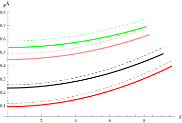
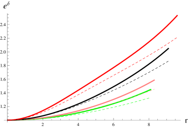
Figure 1: Plots of metric potentials of Tolman IV versus $r$ for Her X-I, LMC X-4, 4U1820-30 and PSR J1614-2230 quark candidates.

4.1 Behavior of State Variables

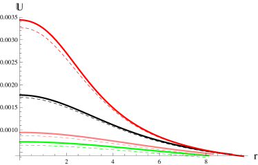
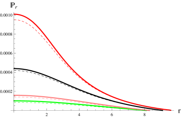
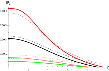
Figure 2: Analysis of energy density, radial/tangential pressures versus $r$ for Her X-I, LMC X-4, 4U1820-30 and PSR J1614-2230 quark candidates.

The mandatory role of physical factors (pressure ingredients, energy density and charge) in immensely dense compact entities cannot be ignored. In order to determine the physical acceptance of these celestial objects, we figure out the contribution of physical variables. The behavior of these quantities guarantees the acceptability if they remain positive as a whole, display maximal value at the center and decrease smoothly as radial coordinate increases. The density profile presented in Figure 2 reveals the denser core and deteriorates when $r$ increases. It can also be noticed that for $\mathcal{Q}=1.5$, the quark stars develop into less dense composition. The pressure ingredients $\mathbb{P}_{r}$ and $\mathbb{P}_{t}$ demonstrate the analogous behavior of density and approach zero at the boundary. The regularity of the proposed solution is achieved by satisfying some requirements at the center, which are shown as

$$\frac{d\mathbb{U}}{dr}|_{r=0}=0,\quad\frac{d\mathbb{P}_{r}}{dr}|_{r=0}=0,\quad\frac{d\mathbb{P}_{t}}{dr}|_{r=0}=0,$$

$$\frac{d^{2}\mathbb{U}}{dr^{2}}|_{r=0}<0,\quad\frac{d^{2}\mathbb{P}_{r}}{dr^{2}}|_{r=0}<0,\quad\frac{d^{2}\mathbb{P}_{t}}{dr^{2}}|_{r=0}<0.$$

From the Figures 3 and 4, one can confirm the regularity of solution as all the considered strange candidates fulfill the regularity conditions under the impact of both charges.

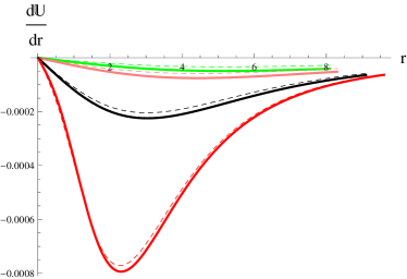
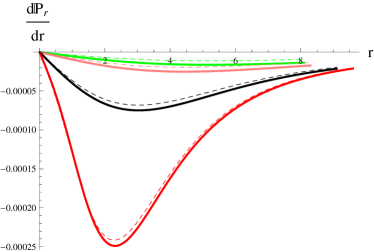
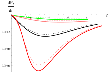
Figure 3: Behavior of $\frac{d\mathbb{U}}{dr}$, $\frac{d\mathbb{P}_{r}}{dr}$ and $\frac{d\mathbb{P}_{t}}{dr}$ versus $r$ for Her X-I, LMC X-4, 4U1820-30 and PSR J1614-2230 quark candidates.

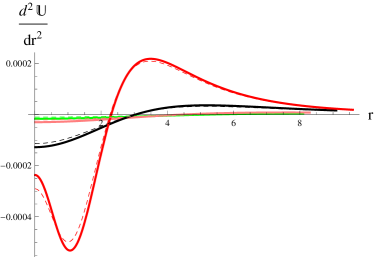
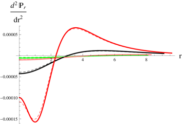
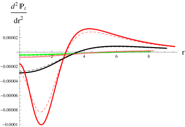
Figure 4: Behavior of $\frac{d^{2}\mathbb{U}}{dr^{2}}$, $\frac{d^{2}\mathbb{P}_{r}}{dr^{2}}$ and $\frac{d^{2}\mathbb{P}_{t}}{dr^{2}}$ versus $r$ for Her X-I, LMC X-4, 4U1820-30 and PSR J1614-2230 quark candidates.

4.2 Anisotropic and Essential Factors

The anisotropy in the system is generated due to the existence of radial and transversal pressures and is denoted as $\Delta=\mathbb{P}_{t}-\mathbb{P}_{r}$. The anisotropic factor is derived on the basis of pressure components (given in Appendix A) corresponding to Tolman IV solution and bag constant, leading to following expression

$$\Delta =\frac{1}{4r^{4}\big{(}2r^{2}+\mathfrak{X}^{2}\big{)}^{7}\mathfrak{Z}^{8}(\varrho+6\pi)(\varrho+8\pi)}\{3\big{(}64\mathfrak{B}_{c}\pi^{2}r^{4}\big{(}2r^{2}+\mathfrak{X}^{2}\big{)}^{7}\mathfrak{Z}^{8}$$

$$+\varrho\big{(}64\big{(}4\mathfrak{B}_{c}\varrho\mathfrak{Z}^{8}-3\mathfrak{Z}^{6}+36\big{)}r^{18}+64\big{(}2\big{(}7\mathfrak{B}_{c}\varrho\mathfrak{Z}^{8}-5\mathfrak{Z}^{6}+57\big{)}\mathfrak{X}^{2}+\mathfrak{Z}^{2}\big{(}\mathfrak{Z}^{6}$$

$$-24\big{)}\big{)}r^{16}+16\big{(}\big{(}84\mathfrak{B}_{c}\varrho\mathfrak{Z}^{8}-57\mathfrak{Z}^{6}+528\big{)}\mathfrak{X}^{4}+4\mathfrak{Z}^{2}\big{(}3\mathfrak{Z}^{6}-136\big{)}\mathfrak{X}^{2}-8\mathfrak{Z}^{4}$$

$$\times\big{(}\mathcal{Q}^{2}\mathfrak{Z}^{4}+22\big{)}\big{)}r^{14}+16\big{(}\big{(}70\mathfrak{B}_{c}\varrho\mathfrak{Z}^{8}-45\mathfrak{Z}^{6}+592\big{)}\mathfrak{X}^{6}+5\mathfrak{Z}^{2}\big{(}3\mathfrak{Z}^{6}$$

$$+104\big{)}\mathfrak{X}^{4}-28\mathfrak{Z}^{4}\big{(}\mathcal{Q}^{2}\mathfrak{Z}^{4}-46\big{)}\mathfrak{X}^{2}+192\mathfrak{Z}^{6}\big{)}r^{12}+4\big{(}\big{(}140\mathfrak{B}_{c}\varrho\mathfrak{Z}^{8}-85\mathfrak{Z}^{6}$$

$$+1408\big{)}\mathfrak{X}^{8}+8\mathfrak{Z}^{2}\big{(}5\mathfrak{Z}^{6}-72\big{)}\mathfrak{X}^{6}-8\mathfrak{Z}^{4}\big{(}21\mathcal{Q}^{2}\mathfrak{Z}^{4}+982\big{)}\mathfrak{X}^{4}-12224\mathfrak{Z}^{6}\mathfrak{X}^{2}\big{)}r^{10}$$

$$+4\mathfrak{X}^{2}\big{(}\big{(}42\mathfrak{B}_{c}\varrho\mathfrak{Z}^{8}-24\mathfrak{Z}^{6}-512\big{)}\mathfrak{X}^{8}+\mathfrak{Z}^{2}\big{(}15\mathfrak{Z}^{6}-5984\big{)}\mathfrak{X}^{6}-28\mathfrak{Z}^{4}\big{(}5\mathcal{Q}^{2}\mathfrak{Z}^{4}$$

$$+442\big{)}\mathfrak{X}^{4}-3904\mathfrak{Z}^{6}\mathfrak{X}^{2}+8064\mathfrak{Z}^{8}\big{)}r^{8}+\mathfrak{X}^{4}\mathfrak{Z}^{2}\big{(}\mathfrak{Z}^{4}\big{(}28\mathfrak{B}_{c}\mathfrak{Z}^{2}\varrho-15\big{)}\mathfrak{X}^{8}$$

$$+4\big{(}3\mathfrak{Z}^{6}+704\big{)}\mathfrak{X}^{6}-280\mathfrak{Z}^{2}\big{(}\mathcal{Q}^{2}\mathfrak{Z}^{4}-80\big{)}\mathfrak{X}^{4}+47936\mathfrak{Z}^{4}\mathfrak{X}^{2}+32832\mathfrak{Z}^{6}\big{)}r^{6}$$

$$+\mathfrak{X}^{6}\mathfrak{Z}^{4}\big{(}\mathfrak{Z}^{2}\big{(}2\mathfrak{B}_{c}\mathfrak{Z}^{2}\varrho-1\big{)}\mathfrak{X}^{8}+\mathfrak{Z}^{4}\mathfrak{X}^{6}-4\big{(}21\mathcal{Q}^{2}\mathfrak{Z}^{4}+184\big{)}\mathfrak{X}^{4}-3776\mathfrak{Z}^{2}\mathfrak{X}^{2}$$

$$-4320\mathfrak{Z}^{4}\big{)}r^{4}-14\mathcal{Q}^{2}\mathfrak{X}^{12}\mathfrak{Z}^{8}r^{2}-\mathcal{Q}^{2}\mathfrak{X}^{14}\mathfrak{Z}^{8}\big{)}+4\pi\big{(}384\big{(}2\mathfrak{B}_{c}\varrho\mathfrak{Z}^{8}-\mathfrak{Z}^{6}$$

$$+12\big{)}r^{18}+32\big{(}\big{(}84\mathfrak{B}_{c}\varrho\mathfrak{Z}^{8}-41\mathfrak{Z}^{6}+480\big{)}\mathfrak{X}^{2}+2\mathfrak{Z}^{2}\big{(}\mathfrak{Z}^{6}-24\big{)}\big{)}r^{16}+16$$

$$\times\big{(}\big{(}252\mathfrak{B}_{c}\varrho\mathfrak{Z}^{8}-121\mathfrak{Z}^{6}+1088\big{)}\mathfrak{X}^{4}+2\mathfrak{Z}^{2}\big{(}5\mathfrak{Z}^{6}-536\big{)}\mathfrak{X}^{2}-16\mathfrak{Z}^{4}\big{(}\mathcal{Q}^{2}\mathfrak{Z}^{4}$$

$$+28\big{)}\big{)}r^{14}+32\big{(}\big{(}105\mathfrak{B}_{c}\varrho\mathfrak{Z}^{8}-50\mathfrak{Z}^{6}+664\big{)}\mathfrak{X}^{6}+\mathfrak{Z}^{2}\big{(}5\mathfrak{Z}^{6}+848\big{)}\mathfrak{X}^{4}-4\mathfrak{Z}^{4}$$

$$\times\big{(}7\mathcal{Q}^{2}\mathfrak{Z}^{4}-410\big{)}\mathfrak{X}^{2}+160\mathfrak{Z}^{6}\big{)}r^{12}+16\big{(}\big{(}105\mathfrak{B}_{c}\varrho\mathfrak{Z}^{8}-50\mathfrak{Z}^{6}+1024\big{)}\mathfrak{X}^{8}$$

$$+\mathfrak{Z}^{2}\big{(}5\mathfrak{Z}^{6}+1088\big{)}\mathfrak{X}^{6}-28\mathfrak{Z}^{4}\big{(}3\mathcal{Q}^{2}\mathfrak{Z}^{4}+94\big{)}\mathfrak{X}^{4}-6464\mathfrak{Z}^{6}\mathfrak{X}^{2}\big{)}r^{10}+2\mathfrak{X}^{2}$$

$$\times\big{(}\big{(}252\mathfrak{B}_{c}\varrho\mathfrak{Z}^{8}-121\mathfrak{Z}^{6}-1280\big{)}\mathfrak{X}^{8}+2\mathfrak{Z}^{2}\big{(}5\mathfrak{Z}^{6}-11712\big{)}\mathfrak{X}^{6}-16\mathfrak{Z}^{4}$$

$$\times\big{(}35\mathcal{Q}^{2}\mathfrak{Z}^{4}+3732\big{)}\mathfrak{X}^{4}-35392\mathfrak{Z}^{6}\mathfrak{X}^{2}+25344\mathfrak{Z}^{8}\big{)}r^{8}+\mathfrak{X}^{4}\big{(}\big{(}84\mathfrak{B}_{c}\varrho\mathfrak{Z}^{8}$$

$$-41\mathfrak{Z}^{6}-1024\big{)}\mathfrak{X}^{8}+2\mathfrak{Z}^{2}\big{(}\mathfrak{Z}^{6}-1408\big{)}\mathfrak{X}^{6}+\big{(}20992\mathfrak{Z}^{4}-560\mathcal{Q}^{2}\mathfrak{Z}^{8}\big{)}\mathfrak{X}^{4}$$

$$+69824\mathfrak{Z}^{6}\mathfrak{X}^{2}+57600\mathfrak{Z}^{8}\big{)}r^{6}+3\mathfrak{X}^{6}\mathfrak{Z}^{2}\big{(}\mathfrak{Z}^{4}\big{(}2\mathfrak{B}_{c}\mathfrak{Z}^{2}\varrho-1\big{)}\mathfrak{X}^{8}+256\mathfrak{X}^{6}$$

$$-8\mathfrak{Z}^{2}\big{(}7\mathcal{Q}^{2}\mathfrak{Z}^{4}-128\big{)}\mathfrak{X}^{4}+448\mathfrak{Z}^{4}\mathfrak{X}^{2}-960\mathfrak{Z}^{6}\big{)}r^{4}-28\mathcal{Q}^{2}\mathfrak{X}^{12}\mathfrak{Z}^{8}r^{2}$$

$$-2\mathcal{Q}^{2}\mathfrak{X}^{14}\mathfrak{Z}^{8}\big{)}\big{)}\}^{-1}.$$ (35)

Using the observational data presented in Table 1, we investigate how anisotropy affects the structural progression of spherical matter source. When the tangential pressure is smaller than radial pressure ($\mathbb{P}_{t}<\mathbb{P}_{r}$), it indicates $\Delta<0$ and pressure is applied in the inward direction. The expression $\Delta>0$ is attained for $\mathbb{P}_{t}>\mathbb{P}_{r}$ implying that anisotropic pressure is in the outward direction. For $\mathcal{Q}=0.1$, the anisotropy of the stars Her X-I, LMC X-4 and 4U1820-30 is negative at first and then becomes positive, however, PSR J1614-2230 shows negative anisotropy in the whole domain. When $\mathcal{Q}=1.5$, the stellar candidates Her X-I and LMC X-4 have positive anisotropic pressure throughout, whereas the anisotropy of 4U1820-30 and PSR J1614-2230 transforms from negative to positive (Figure 5).

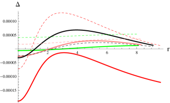
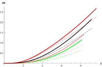
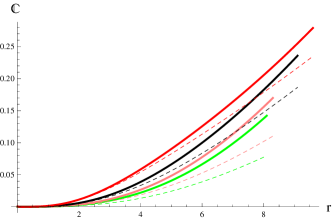
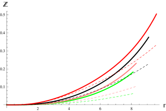
Figure 5: Plots of anisotropy, mass, compactness and redshift versus $r$ for Her X-I, LMC X-4, 4U1820-30 and PSR J1614-2230 quark candidates.

One of the essential characteristics of spherical symmetric structure is mass, which is mathematically denoted as

$$\mathit{m}=4\pi\int^{\mathfrak{R}}_{0}\mathbb{U}r^{2}dr,$$ (36)

where $\mathbb{U}$ is expressed in Appendix A. The mass of strange stellar bodies is determined through numerical manipulation of Eq.(36) with $\mathit{m}(0)=0$ as the initial condition. Compactness (the ratio of mass and radius) is another important physical characteristic of celestial objects. Its mathematical formula is given as $\mathbb{C}=\frac{\mathit{m}}{r}$ and is graphically portrayed using the previously mentioned condition. In order to determine the maximum bound of compactness factor, Buchdahl [33] matched the outer and inner regimes of spherical system to conclude that its values should not exceed $\frac{4}{9}$. The astrophysical objects present in vigorous gravitational pull produce enlarged electromagnetic radiation, whose increment in wavelength is measured using redshift factor and is delineated as

$$\mathbb{Z}=\frac{1}{\sqrt{1-2\mathbb{C}}}-1.$$

On the celestial surface of isotropic matter configuration, the maximum range of this factor is $\mathbb{Z}<2$, while it becomes 5.211 for the anisotropic configured source. Figure 5 shows that these factors (mass, compactness and redshift) comply within their required bounds for all the considered objects.

4.3 Energy Constraints

Several mathematical constraints are used to ensure the occurrence of usual matter configuration present in the internal regime of cosmic bodies. These restrictions are known as energy conditions and have proven to be interesting criterion that differentiate between exotic and normal matter sources. The accomplishment of these limitations indicates regular source and signifies the viability of the resulting solution. These requirements, for the anisotropic configuration, are classified into null (NEC), dominant (DEC), strong (SEC) and weak energy condition (WEC), respectively, as

NEC: $$\mathbb{U}+\mathbb{P}_{r}\geq 0,\quad\mathbb{U}+\mathbb{P}_{t}+\frac{q^{2}}{4\pi r^{4}}\geq 0,$$

DEC: $$\mathbb{U}-\mathbb{P}_{t}\geq 0,\quad\mathbb{U}-\mathbb{P}_{r}+\frac{q^{2}}{4\pi r^{4}}\geq 0,$$

SEC: $$\mathbb{U}+\mathbb{P}_{r}+2\mathbb{P}_{t}+\frac{q^{2}}{4\pi r^{4}}\geq 0,$$

WEC: $$\mathbb{U}+\frac{q^{2}}{8\pi r^{4}}\geq 0,\quad\mathbb{U}+\mathbb{P}_{r}\geq 0,\quad\mathbb{U}+\mathbb{P}_{t}+\frac{q^{2}}{4\pi r^{4}}\geq 0.$$ (37)

The energy constraints corresponding to all compact structures under the influence of electromagnetic field are graphically analyzed in Figure 6. It can be observed that both the solution and stars depict realistic behavior in the present work for both $\mathcal{Q}=0.1$ and $1.5$. This shows that all the strange quark candidates incorporate ordinary matter internally.

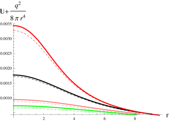
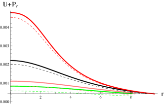
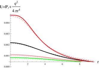
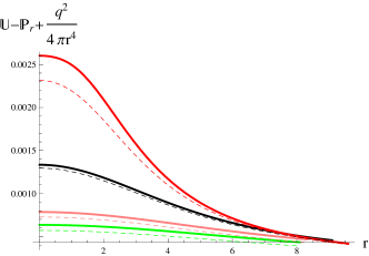
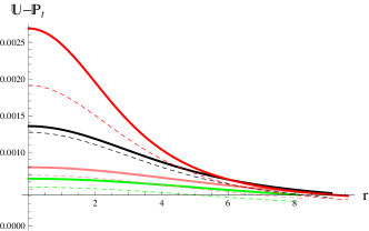
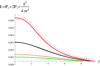
Figure 6: Behavior of energy constraints versus $r$ for Her X-I, LMC X-4, 4U1820-30 and PSR J1614-2230 quark candidates.

4.4 Stability Conditions

The stability of anisotropic stellar structures is an important topic of discussion in the background of astrophysical world. One such method to estimate the stable nature of quark compositions is regarded as adiabatic index of the form

$$\Gamma_{r}=\frac{\mathbb{U}+\mathbb{P}_{r}}{\mathbb{P}_{r}}\bigg{(}\frac{d\mathbb{P}_{r}}{d\mathbb{U}}\bigg{)},\quad\Gamma_{t}=\frac{\mathbb{U}+\mathbb{P}_{t}}{\mathbb{P}_{t}}\bigg{(}\frac{d\mathbb{P}_{t}}{d\mathbb{U}}\bigg{)},$$ (38)

where $\Gamma_{r}$ and $\Gamma_{t}$ are its radial and temporal components, whose values must be greater than $\frac{4}{3}$ to depict the stable distributions [39]. In addition to this, the causality condition is an alternative approach according to which the speed of light exceeds the speed of sound. The radial and transverse velocities, respectively, are two components described by $\mathbb{V}^{2}_{r}$ and $\mathbb{V}^{2}_{t}$. For the stable configuration, these constituents must fulfill the conditions $0<\mathbb{V}^{2}_{r}<1$ and $0<\mathbb{V}^{2}_{t}<1$, and they are mathematically expressed as

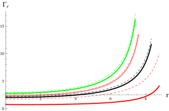
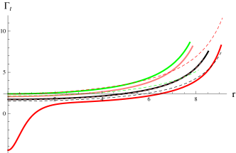
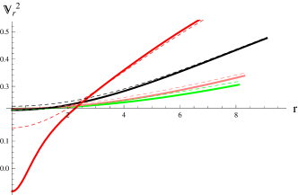
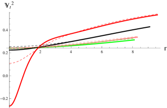
Figure 7: Behavior of adiabatic index and causality condition versus $r$ for Her X-I, LMC X-4, 4U1820-30 and PSR J1614-2230 quark candidates.

$$\mathbb{V}^{2}_{r}=\frac{d\mathbb{P}_{r}}{d\mathbb{U}},\quad\quad\mathbb{V}^{2}_{t}=\frac{d\mathbb{P}_{t}}{d\mathbb{U}}.$$ (39)

In other words, we can also say that both the aforementioned components must lie between the range of 0 and 1 [40]. Figure 7 exhibits both criteria, from which we can notice that all the stellar stars meet the necessary requisites for $\mathcal{Q}=0.1$. For the higher charge value, the candidates Her X-I, 4U1820-30 and LMC X-4 portray the stable structures whereas PSR J1614-2230 becomes inconsistent through both techniques as not satisfying the required limits (Figure 7).

5 Conclusion

The main motivation of this paper is to study the role of electromagnetic field on the substantial features of Her X-I, PSR J1614-2230, 4U1820-30 and LMC X-4. In this regard, we have considered the static spherical compositions occupying anisotropic source in their interior. The modified field equations are formulated using the quadratic model $f(G,T)=G^{2}+\varrho T$ of $f(G,T)$ gravity. The radial pressure and density are interlinked with bag constant in the MIT bag model EoS which transforms the modified field equations in terms of $\mathfrak{B}_{c}$. The radial and temporal metric potentials of Tolman IV solution have been used to find the anisotropic solution with $\mathfrak{X}^{2}$, $\mathfrak{C}^{2}$ and $\mathfrak{Z}^{2}$ as unknowns. The interior spacetime is matched with the Reissner-Nordstr$\ddot{o}$m metric (chosen as outer geometry) to compute these unknown variables. Further, the boundary conditions represent these constants into masses and radii of the proposed quark stars. The expression of $\mathbb{P}_{r}$ in Appendix A yields the bag constant equation through which we have evaluated the value of $\mathfrak{B}_{c}$ for each strange star corresponding to $\mathcal{Q}=0.1$ and 1.5 (Tables 2 and 3) by using their observational data. The graphical analysis of all the considered compact bodies have been discussed for two values of charge.

The physical entities (energy density and pressure components) have shown the acceptable behavior, i.e., the maximal values at the center which decrease gradually with increasing $r$. The compatibility of the solution has been confirmed through the behavior of metric potentials (Figure 1). The viability of all quark candidates has been investigated through energy conditions that ensure the occurrence of regular matter within these stars corresponding to both charges. It is also found that compactness, mass and redshift factors satisfy their necessary ranges. The stellar compact objects Her X-I, LMC X-4 and 4U1820-30 depict the stable nature for both charges as they meet the confined bounds. The star candidate PSR J1614-2230 portrays a stable structure when $\mathcal{Q}=0.1$, but becomes unstable for $\mathcal{Q}=1.5$. In GR [41], the stars LMC X-4 and Her X-I were found to be more denser in comparison to this present work. However, one can also notice that more appropriate results are established for 4U1820-30 as compared to [42]. Sharif et al [43] established a viable and stable charged 4U 1608-52 star by assuming two particular values of $\mathfrak{B}_{c}$ in $f(G,T)$ gravity. It is found that the proposed solutions reduce to GR when $\varrho=\varsigma=0$ is imposed on the model (11).

Appendix A

The physical variables corresponding to unknowns involved in Tolman IV solution are

$$\mathbb{U} =\frac{1}{2\mathfrak{Z}^{8}(\varrho+8\pi)\big{(}\mathfrak{X}^{2}+2r^{2}\big{)}^{7}}\{\mathfrak{X}^{6}\mathfrak{Z}^{2}\big{(}6\mathfrak{X}^{6}\big{(}\mathfrak{Z}^{6}-384\big{)}-13632\mathfrak{X}^{4}\mathfrak{Z}^{2}$$

$$-26688\mathfrak{X}^{2}\mathfrak{Z}^{4}+\mathfrak{X}^{8}\mathfrak{Z}^{4}\big{(}2\mathfrak{B}_{c}\mathfrak{Z}^{2}(\varrho+8\pi)+3\big{)}-17280\mathfrak{Z}^{6}\big{)}+256\mathfrak{B}_{c}\mathfrak{Z}^{8}(\varrho$$

$$+8\pi)r^{14}+32r^{12}\big{(}\mathfrak{X}^{2}\big{(}28\mathfrak{B}_{c}\mathfrak{Z}^{8}(\varrho+8\pi)+3\mathfrak{Z}^{6}-72\big{)}+6\mathfrak{Z}^{2}\big{(}\mathfrak{Z}^{6}-24\big{)}\big{)}$$

$$+48r^{10}\big{(}2\mathfrak{X}^{2}\mathfrak{Z}^{2}\big{(}7\mathfrak{Z}^{6}-8\big{)}+\mathfrak{X}^{4}\big{(}28\mathfrak{B}_{c}\mathfrak{Z}^{8}(\varrho+8\pi)+7\mathfrak{Z}^{6}-32\big{)}+96\mathfrak{Z}^{4}\big{)}$$

$$+32r^{8}\big{(}6\mathfrak{X}^{4}\mathfrak{Z}^{2}\big{(}5\mathfrak{Z}^{6}-164\big{)}-1056\mathfrak{X}^{2}\mathfrak{Z}^{4}+\mathfrak{X}^{6}\big{(}35\mathfrak{B}_{c}\mathfrak{Z}^{8}(\varrho+8\pi)+15\mathfrak{Z}^{6}$$

$$-216\big{)}+96\mathfrak{Z}^{6}\big{)}+8r^{6}\big{(}\mathfrak{X}^{6}\big{(}90\mathfrak{Z}^{8}-8256\mathfrak{Z}^{2}\big{)}-7776\mathfrak{X}^{4}\mathfrak{Z}^{4}+2112\mathfrak{X}^{2}\mathfrak{Z}^{6}$$

$$+5\mathfrak{X}^{8}\big{(}14\mathfrak{B}_{c}\mathfrak{Z}^{8}(\varrho+8\pi)+9\mathfrak{Z}^{6}-384\big{)}\big{)}+6\mathfrak{X}^{2}r^{4}\big{(}\mathfrak{X}^{6}\big{(}50\mathfrak{Z}^{8}-512\mathfrak{Z}^{2}\big{)}$$

$$+10208\mathfrak{X}^{4}\mathfrak{Z}^{4}+19776\mathfrak{X}^{2}\mathfrak{Z}^{6}+\mathfrak{X}^{8}\big{(}28\mathfrak{B}_{c}\mathfrak{Z}^{8}(\varrho+8\pi)+25\mathfrak{Z}^{6}-768\big{)}$$

$$+6912\mathfrak{Z}^{8}\big{)}+\mathfrak{X}^{4}r^{2}\big{(}66\mathfrak{X}^{6}\mathfrak{Z}^{2}\big{(}\mathfrak{Z}^{6}+384\big{)}+71424\mathfrak{X}^{4}\mathfrak{Z}^{4}+78144\mathfrak{X}^{2}\mathfrak{Z}^{6}$$

$$+\mathfrak{X}^{8}\big{(}28\mathfrak{B}_{c}\mathfrak{Z}^{8}(\varrho+8\pi)+33\mathfrak{Z}^{6}+3072\big{)}+24192\mathfrak{Z}^{8}\big{)}\}^{-1},$$

$$\mathbb{P}_{r} =-\frac{1}{2\mathfrak{Z}^{8}(\varrho+8\pi)\big{(}\mathfrak{X}^{2}+2r^{2}\big{)}^{7}}\{\mathfrak{X}^{6}\mathfrak{Z}^{2}\big{(}-2\mathfrak{X}^{6}\big{(}\mathfrak{Z}^{6}-384\big{)}+4544\mathfrak{X}^{4}\mathfrak{Z}^{2}$$

$$+8896\mathfrak{X}^{2}\mathfrak{Z}^{4}+\mathfrak{X}^{8}\mathfrak{Z}^{4}\big{(}2\mathfrak{B}_{c}\mathfrak{Z}^{2}(\varrho+8\pi)-1\big{)}+5760\mathfrak{Z}^{6}\big{)}+256\mathfrak{B}_{c}\mathfrak{Z}^{8}(\varrho$$

$$+8\pi)r^{14}+32r^{12}\big{(}\mathfrak{X}^{2}\big{(}28\mathfrak{B}_{c}\mathfrak{Z}^{8}(\varrho+8\pi)-\mathfrak{Z}^{6}+24\big{)}-2\mathfrak{Z}^{2}\big{(}\mathfrak{Z}^{6}-24\big{)}\big{)}$$

$$+16r^{10}\big{(}-2\mathfrak{X}^{2}\mathfrak{Z}^{2}\big{(}7\mathfrak{Z}^{6}-8\big{)}+\mathfrak{X}^{4}\big{(}84\mathfrak{B}_{c}\mathfrak{Z}^{8}(\varrho+8\pi)-7\mathfrak{Z}^{6}+32\big{)}-96\mathfrak{Z}^{4}\big{)}$$

$$+32r^{8}\big{(}\mathfrak{X}^{4}\big{(}328\mathfrak{Z}^{2}-10\mathfrak{Z}^{8}\big{)}+352\mathfrak{X}^{2}\mathfrak{Z}^{4}+\mathfrak{X}^{6}\big{(}35\mathfrak{B}_{c}\mathfrak{Z}^{8}(\varrho+8\pi)-5\mathfrak{Z}^{6}+72\big{)}$$

$$-32\mathfrak{Z}^{6}\big{)}+8r^{6}\big{(}\mathfrak{X}^{6}\big{(}2752\mathfrak{Z}^{2}-30\mathfrak{Z}^{8}\big{)}+2592\mathfrak{X}^{4}\mathfrak{Z}^{4}-704\mathfrak{X}^{2}\mathfrak{Z}^{6}+5\mathfrak{X}^{8}\big{(}14\mathfrak{B}_{c}\mathfrak{Z}^{8}$$

$$\times(\varrho+8\pi)-3\mathfrak{Z}^{6}+128\big{)}\big{)}+2\mathfrak{X}^{2}r^{4}\big{(}\mathfrak{X}^{6}\big{(}512\mathfrak{Z}^{2}-50\mathfrak{Z}^{8}\big{)}-10208\mathfrak{X}^{4}\mathfrak{Z}^{4}$$

$$-19776\mathfrak{X}^{2}\mathfrak{Z}^{6}+\mathfrak{X}^{8}\big{(}84\mathfrak{B}_{c}\mathfrak{Z}^{8}(\varrho+8\pi)-25\mathfrak{Z}^{6}+768\big{)}-6912\mathfrak{Z}^{8}\big{)}-\mathfrak{X}^{4}r^{2}$$

$$\times\big{(}22\mathfrak{X}^{6}\mathfrak{Z}^{2}\big{(}\mathfrak{Z}^{6}+384\big{)}+23808\mathfrak{X}^{4}\mathfrak{Z}^{4}+26048\mathfrak{X}^{2}\mathfrak{Z}^{6}+\mathfrak{X}^{8}\big{(}-28\mathfrak{B}_{c}\mathfrak{Z}^{8}(\varrho+8\pi)$$

$$+11\mathfrak{Z}^{6}+1024\big{)}+8064\mathfrak{Z}^{8}\big{)}\}^{-1},$$

$$\mathbb{P}_{t} =\frac{1}{4r^{4}\big{(}2r^{2}+\mathfrak{X}^{2}\big{)}^{7}\mathfrak{Z}^{8}(\varrho+6\pi)(\varrho+8\pi)}\{8\pi\big{(}64\big{(}4\mathfrak{B}_{c}\varrho\mathfrak{Z}^{8}-9\mathfrak{Z}^{6}+108\big{)}r^{18}$$

$$+64\big{(}2\big{(}7\mathfrak{B}_{c}\varrho\mathfrak{Z}^{8}-15\mathfrak{Z}^{6}+171\big{)}\mathfrak{X}^{2}+3\mathfrak{Z}^{2}\big{(}\mathfrak{Z}^{6}-24\big{)}\big{)}r^{16}+48\big{(}\big{(}28\mathfrak{B}_{c}\varrho\mathfrak{Z}^{8}$$

$$-57\mathfrak{Z}^{6}+528\big{)}\mathfrak{X}^{4}+4\mathfrak{Z}^{2}\big{(}3\mathfrak{Z}^{6}-136\big{)}\mathfrak{X}^{2}-8\mathfrak{Z}^{4}\big{(}q^{2}\mathfrak{Z}^{4}+22\big{)}\big{)}r^{14}+16\big{(}\big{(}70\mathfrak{B}_{c}$$

$$\times\varrho\mathfrak{Z}^{8}-135\mathfrak{Z}^{6}+1776\big{)}\mathfrak{X}^{6}+15\mathfrak{Z}^{2}\big{(}3\mathfrak{Z}^{6}+104\big{)}\mathfrak{X}^{4}-84\mathfrak{Z}^{4}\big{(}q^{2}\mathfrak{Z}^{4}-46\big{)}\mathfrak{X}^{2}$$

$$+576\mathfrak{Z}^{6}\big{)}r^{12}+4\big{(}\big{(}140\mathfrak{B}_{c}\varrho\mathfrak{Z}^{8}-255\mathfrak{Z}^{6}+4224\big{)}\mathfrak{X}^{8}+24\mathfrak{Z}^{2}\big{(}5\mathfrak{Z}^{6}-72\big{)}\mathfrak{X}^{6}$$

$$-24\mathfrak{Z}^{4}\big{(}21q^{2}\mathfrak{Z}^{4}+982\big{)}\mathfrak{X}^{4}-36672\mathfrak{Z}^{6}\mathfrak{X}^{2}\big{)}r^{10}+12\mathfrak{X}^{2}\big{(}2\big{(}7\mathfrak{B}_{c}\varrho\mathfrak{Z}^{8}-12\mathfrak{Z}^{6}$$

$$-256\big{)}\mathfrak{X}^{8}+\mathfrak{Z}^{2}\big{(}15\mathfrak{Z}^{6}-5984\big{)}\mathfrak{X}^{6}-28\mathfrak{Z}^{4}\big{(}5q^{2}\mathfrak{Z}^{4}+442\big{)}\mathfrak{X}^{4}-3904\mathfrak{Z}^{6}\mathfrak{X}^{2}$$

$$+8064\mathfrak{Z}^{8}\big{)}r^{8}+\mathfrak{X}^{4}\mathfrak{Z}^{2}\big{(}\mathfrak{Z}^{4}\big{(}28\mathfrak{B}_{c}\mathfrak{Z}^{2}\varrho-45\big{)}\mathfrak{X}^{8}+12\big{(}3\mathfrak{Z}^{6}+704\big{)}\mathfrak{X}^{6}-840\mathfrak{Z}^{2}$$

$$\times\big{(}q^{2}\mathfrak{Z}^{4}-80\big{)}\mathfrak{X}^{4}+143808\mathfrak{Z}^{4}\mathfrak{X}^{2}+98496\mathfrak{Z}^{6}\big{)}r^{6}+\mathfrak{X}^{6}\mathfrak{Z}^{4}\big{(}\mathfrak{Z}^{2}\big{(}2\mathfrak{B}_{c}\mathfrak{Z}^{2}\varrho-3\big{)}\mathfrak{X}^{8}$$

$$+3\mathfrak{Z}^{4}\mathfrak{X}^{6}-12\big{(}21q^{2}\mathfrak{Z}^{4}+184\big{)}\mathfrak{X}^{4}-11328\mathfrak{Z}^{2}\mathfrak{X}^{2}-12960\mathfrak{Z}^{4}\big{)}r^{4}-42q^{2}\mathfrak{X}^{12}\mathfrak{Z}^{8}r^{2}$$

$$-3q^{2}\mathfrak{X}^{14}\mathfrak{Z}^{8}\big{)}+\varrho\big{(}64\big{(}4\mathfrak{B}_{c}\varrho\mathfrak{Z}^{8}-9\mathfrak{Z}^{6}+108\big{)}r^{18}+64\big{(}\big{(}14\mathfrak{B}_{c}\varrho\mathfrak{Z}^{8}-29\mathfrak{Z}^{6}$$

$$+318\big{)}\mathfrak{X}^{2}+5\mathfrak{Z}^{2}\big{(}\mathfrak{Z}^{6}-24\big{)}\big{)}r^{16}+16\big{(}\big{(}84\mathfrak{B}_{c}\varrho\mathfrak{Z}^{8}-157\mathfrak{Z}^{6}+1520\big{)}\mathfrak{X}^{4}$$

$$+64\mathfrak{Z}^{2}\big{(}\mathfrak{Z}^{6}-26\big{)}\mathfrak{X}^{2}-24\mathfrak{Z}^{4}\big{(}q^{2}\mathfrak{Z}^{4}+14\big{)}\big{)}r^{14}+16\big{(}\big{(}70\mathfrak{B}_{c}\varrho\mathfrak{Z}^{8}-115\mathfrak{Z}^{6}$$

$$+1488\big{)}\mathfrak{X}^{6}+\mathfrak{Z}^{2}\big{(}85\mathfrak{Z}^{6}+248\big{)}\mathfrak{X}^{4}+\big{(}2456\mathfrak{Z}^{4}-84q^{2}\mathfrak{Z}^{8}\big{)}\mathfrak{X}^{2}+704\mathfrak{Z}^{6}\big{)}r^{12}$$

$$+4\big{(}\big{(}1664+140\mathfrak{B}_{c}\varrho\mathfrak{Z}^{8}-195\mathfrak{Z}^{6}\big{)}\mathfrak{X}^{8}+16\mathfrak{Z}^{2}\big{(}15\mathfrak{Z}^{6}-796\big{)}\mathfrak{X}^{6}-168\mathfrak{Z}^{4}$$

$$\times\big{(}3q^{2}\mathfrak{Z}^{4}+202\big{)}\mathfrak{X}^{4}-33856\mathfrak{Z}^{6}\mathfrak{X}^{2}\big{)}r^{10}+4\mathfrak{X}^{2}\big{(}\big{(}42\mathfrak{B}_{c}\varrho\mathfrak{Z}^{8}-2304-47\mathfrak{Z}^{6}\big{)}$$

$$\times\mathfrak{X}^{8}+\mathfrak{Z}^{2}\big{(}95\mathfrak{Z}^{6}-18464\big{)}\mathfrak{X}^{6}-20\mathfrak{Z}^{4}\big{(}21q^{2}\mathfrak{Z}^{4}+1346\big{)}\mathfrak{X}^{4}+8064\mathfrak{Z}^{6}\mathfrak{X}^{2}$$

$$+31104\mathfrak{Z}^{8}\big{)}r^{8}+\mathfrak{X}^{4}\big{(}\big{(}28\mathfrak{B}_{c}\varrho\mathfrak{Z}^{8}-23\mathfrak{Z}^{6}+2048\big{)}\mathfrak{X}^{8}+16\mathfrak{Z}^{2}\big{(}5\mathfrak{Z}^{6}+1584\big{)}\mathfrak{X}^{6}$$

$$-24\mathfrak{Z}^{4}\big{(}35q^{2}\mathfrak{Z}^{4}-4784\big{)}\mathfrak{X}^{4}+195904\mathfrak{Z}^{6}\mathfrak{X}^{2}+114624\mathfrak{Z}^{8}\big{)}r^{6}+\mathfrak{X}^{6}\mathfrak{Z}^{2}\big{(}\mathfrak{Z}^{4}$$

$$\times\big{(}2\mathfrak{B}_{c}\mathfrak{Z}^{2}\varrho-1\big{)}\mathfrak{X}^{8}+\big{(}7\mathfrak{Z}^{6}-1536\big{)}\mathfrak{X}^{6}-4\mathfrak{Z}^{2}\big{(}63q^{2}\mathfrak{Z}^{4}+2824\big{)}\mathfrak{X}^{4}$$

$$-29120\mathfrak{Z}^{4}\mathfrak{X}^{2}-24480\mathfrak{Z}^{6}\big{)}r^{4}-42q^{2}\mathfrak{X}^{12}\mathfrak{Z}^{8}r^{2}-3q^{2}\mathfrak{X}^{14}\mathfrak{Z}^{8}\big{)}\}^{-1}.$$

References

- [1] W. Baade, F. Zwicky, Remarks on super-novae and cosmic rays, Phys. Rev. 46 (1934) 76, https://doi.org/10.1103/Phys. Rev.46.76.2.
- [2] E. Witten, Cosmic separation of phases, Phys. Rev. D 30 (1984) 272, https://doi.10.1103/physrevd.30.272; X.D. Li, Z.G. Dai, Z.R. Wang, Is Her X-1 a strange star?, Astron. Astrophys. 303 (1995) L1; I. Bombaci, Observational evidence for strange matter in compact objects from the x-ray burster 4U 1820-30, Phys. Rev. C 55 (1997) 1587, https://doi.org/10.1103/Phys Rev C.55.1587.
- [3] M. Ruderman, Pulsars: structure and dynamics, Annu. Rev. Astron. Astrophys. 10 (1972) 427, https://doi.org/10.1146/annurev.aa.10.090172.002235.
- [4] K. Dev, M. Gleiser, Anisotropic stars: exact solutions, Gen. Relativ. Grav. 34 (2002) 1793, 0001-7701/02/1100-1793/0.
- [5] S.K.M. Hossein, et al., Anisotropic compact stars with variable cosmological constant, Int. J. Mod. Phys. D 21 (2012) 1250088, https://doi.org/10.1142/S0218271812500885.
- [6] M. Kalam, et al., Anisotropic quintessence stars, Astrophys. Space Sci. 349 (2014) 865, http://doi.10.1007/s10509-013-1677-x.
- [7] S.K. Maurya, et al., Generalised model for anisotropic compact stars, Eur. Phys. J. C 76 (2016) 693, http://doi 10.1140/epjc/s10052-016-4527-5.
- [8] M.H. Murad, Some analytical models of anisotropic strange stars, Astrophys. Space Sci. 361 (2016) 20, http://doi 10.1007/s10509-015-2582-2.
- [9] K.D. Matondo, S.D. Maharaj, S. Ray, Charged isotropic model with conformal symmetry, Astrophys. Space Sci. 363 (2018) 187, https://doi.org/10.1007/s10509-018-3410-2.
- [10] P. Mafa Takisa, S.D. Maharaj, L.L. Leeuw, Effect of electric charge on conformal compact stars, Eur. Phys. J. C 79 (2019) 8, https://doi.org/10.1140/epjc/s10052-018-6519-0; S.K. Maurya, F. Tello-Ortiz, Charged anisotropic compact star in gravity: A minimal geometric deformation gravitational decoupling approach, Phys. Dark Universe 27 (2020) 100442, https://doi.org/10.1016/j.dark.2019.100442; G. Panotopoulos, et al., Charged polytropic compact stars in 4D Einstein Gauss-Bonnet gravity, Chin. J. Phys. 77 (2022) 2106, https://doi.org/10.1016/j.cjph.2022.01.008; M. Sharif, T. Naseer, Influence of charge on extended decoupled anisotropic solutions in gravity, Indian J. Phys. 96 (2022) 4373, https://doi.org/10.1007/s12648-022-02339-7.
- [11] P. Haensel, J.L. Zdunik, R. Schaefer, Strange quark stars, Astron. Astrophys. 160 (1986) 121; F. Weber, Strange quark matter and compact stars, Prog. Part. Nucl. Phys. 54 (2005) 193, https://doi.org/10.1016/j.ppnp.2004.07.001; M.A. Perez Garcia, J. Silk, J.R. Stone, Dark matter, neutron stars, and strange quark matter, Phys. Rev. Lett. 105 (2010) 141101, http://doi: 10.1103/PhysRevLett.105.141101; H. Rodrigues, S.B. Duarte, J.C.T. De Oliveira, Massive compact stars as quark stars, Astrophys. J. 730 (2011) 31, http://doi:10.1088/0004-637X/730/1/31.
- [12] P.B. Demorest, et al., A two-solar-mass neutron star measured using Shapiro delay, Nature 467 (2010) 1081, http://doi:10.1038/nature09466.
- [13] F. Rahaman, et al., A new deterministic model of strange stars, Eur. Phys. J. C 74 (2014) 3126, http://doi 10.1140/epjc/s10052-014-3126-6.
- [14] P. Bhar, A new hybrid star model in Krori-Barua spacetime, Astrophys. Space Sci. 357 (2015) 46, http://doi 10.1007/s10509-015-2271-1.
- [15] D. Deb, et al., Relativistic model for anisotropic strange stars, Ann. Phys. 387 (2017) 239, https://doi.org/10.1016/j.aop.2017.10.010; D. Deb, et al., Anisotropic strange stars in the Einstein-Maxwell spacetime, Eur. Phys. J. C 78 (2018) 465, https://doi.org/10.1140/epjc/s10052-018-5930-x.
- [16] M. Sharif, A. Waseem, Anisotropic quark stars in gravity, Eur. Phys. J. C 78 (2018) 868, https://doi.org/10.1140/epjc/s10052-018-6363-2; Role of curvature-matter coupling on anisotropic strange stars, Chin. J. Phys. 63 (2020) 92, https://doi.org/10.1016/j.cjph.2019.11.006; M. Sharif, A. Majid, Compact stars with MIT bag model in massive Brans-Dicke gravity, Astrophys. Space Sci. 366 (2021) 54, https://doi.org/10.1007/s10509-021-03962-2; A. Majid, M. Sharif, Quark stars in massive Brans Dicke gravity with Tolman Kuchowicz spacetime, Universe 6 (2020) 124, https://doi:10.3390/universe6080124; M. Sharif, T. Naseer, Effects of non-minimal matter-geometry coupling on embedding class-one anisotropic solutions, Phys. Scr. 97 (2022) 055004, https://doi 10.1088/1402-4896/ac5ed4; Study of charged compact stars in non-minimally coupled gravity, Fortschr. Phys. 71 (2022) 2200147, https://doi.org/10.1002/prop.202200147; Study of anisotropic compact stars in gravity, Pramana 96 (2022) 119, https://doi.org/10.1007/s12043-022-02357-4.
- [17] S. Capozziello, A. Stabile, A. Troisi, Spherical symmetry in -gravity Class. Quantum Grav. 25 (2008) 085004, https://doi 10.1088/0264-9381/25/8/085004; S. Capozziello, E. De Filippis, V. Salzano, Modelling clusters of galaxies by gravity, Mon. Not. R. Astron. Soc. 394 (2009) 947, https://doi.org/10.1111/j.1365-2966.2008.14382.x; S. Nojiri, S.D. Odintsov, Unified cosmic history in modified gravity: from theory to Lorentz non-invariant models, Phys. Rep. 505 (2011) 59, https://doi.org/10.1016/j.physrep.2011.04.001.
- [18] M. Sharif, H.R. Kausar, Effects of model on the dynamical instability of expansion free gravitational collapse, J. Cosmol. Astropart. Phys. 07 (2011) 022, https://doi:10.1088/1475-7516/2011/07/022; A.V. Astashenok, S. Capozziello, S.D. Odintsov, Extreme neutron stars from extended theories of gravity, J. Cosmol. Astropart. Phys. 2015 (2015) 001, https://doi:10.1088/1475-7516/2015/01/001; Nonperturbative models of quark stars in gravity, Phys. Lett. B 742 (2015) 160, https://doi.org/10.1016/j.physletb.2015.01.030.
- [19] T. Harko, et al., gravity, Phys. Rev. D 84 (2011) 024020, https://doi.10.1103/PhysRevD.84.024020.
- [20] M. Sharif, M. Zubair, Thermodynamic behavior of particular gravity models, J. Exp. Theor. Phys. 117 (2013) 248, https://doi.10.1134/S1063776113100075; H. Shabani, M. Farhoudi, cosmological models in phase space, Phys. Rev. D 88 (2013) 044048, https://doi.org/10.1103/PhysRevD.88.044048; A. Alhamzawi, R. Alhamzawi, Gravitational lensing by gravity, Int. J. Mod. Phys. D 25 (2016) 1650020, https://doi.org/10.1142/S0218271816500206; M. Sharif, A. Siddiqa, Study of charged stellar structures in gravity, Eur. Phys. J. Plus 132 (2017) 529, https://doi.10.1140/epjp/i2017-11810-4.
- [21] S. Nojiri, S.D. Odintsov, Modified Gauss-Bonnet theory as gravitational alternative for dark energy, Phys. Lett. B 631 (2005) 1, https://doi.org/10.1016/j.physletb.2005.10.010.
- [22] K. Bamba, et al., Finite-time future singularities in modified Gauss-Bonnet and gravity and singularity avoidance, Eur. Phys. J. C 67 (2010) 295, https://doi.10.1140/epjc/s10052-010-1292-8.
- [23] R. Myrzakulov, D. Saez-Gomez, A. Tureanu, On the CDM Universe in gravity, Gen. Relativ. Grav. 43 (2011) 1671, https://doi.10.1007/s10714-011-1149-y.
- [24] M. Sharif, H. Ismat Fatima, Noether symmetries in gravity, J. Exp. Theor. Phys. 122 (2016) 104, https://doi.10.1134/S1063776116010192.
- [25] K. Bamba, et al., Energy conditions in modified gravity, Gen. Relativ. Grav. 49 (2017) 112, https://doi.10.1007/s10714-017-2276-x.
- [26] M. Sharif, A. Ramzan, Anisotropic compact stellar objects in modified Gauss-Bonnet gravity, Phys. Dark Universe 30 (2020) 100737, https://doi.org/10.1016/j.dark.2020.100737.
- [27] M. Sharif, A. Ikram, Energy conditions in gravity, Eur. Phys. J. C 76 (2016) 640, https://doi.10.1140/epjc/s10052-016-4502-1.
- [28] M.F. Shamir, M. Ahmad, Emerging anisotropic compact stars in gravity, Eur. Phys. J. C 77 (2017) 674, https://doi.10.1140/epjc/s10052-017-5239-1.
- [29] S.K. Maurya, et al., Anisotropic stars in gravity under class I space-time, Eur. Phys. J. Plus 135 (2020) 824, https://doi.org/10.1140/epjp/s13360-020-00832-8.
- [30] M. Sharif, A. Naeem, Anisotropic solution for compact objects in gravity, Int. J. Mod. Phys. A 35 (2020) 2050121, https://doi.org/10.1142/S0217751X20501213.
- [31] M. Sharif, K. Hassan, Electromagnetic effects on the complexity of static cylindrical object in gravity, Eur. Phys. J. Plus 137 (2022) 1380, https://doi.org/10.1140/epjp/s13360-022-03612-8; Complexity factor for static cylindrical objects in gravity, Pramana 96 (2022) 50, https://doi.org/10.1007/s12043-022-02298-y; Complexity of dynamical cylindrical system in gravity, Mod. Phys. Lett. A 37 (2022) 2250027, https://doi.org/10.1142/S0217732322500274; Analysis of complexity factor for charged dissipative configuration in modified gravity, Eur. Phys. J. Plus 138 (2023) 787, https://doi.org/10.1140/epjp/s13360-023-04417-z; Complexity for dynamical anisotropic sphere in gravity, Chin. J. Phys 77 (2022) 1479, https://doi.org/10.1016/j.cjph.2021.11.038; Complexity of charged dynamical spherical system in modified gravity, Chin. J. Phys 84 (2023) 152, https://doi.org/10.1016/j.cjph.2023.03.024.
- [32] M. Kalma, et al., A relativistic model for strange quark star, Int. J. Theor. Phys. 52 (2013) 3319, https://doi.10.1007/s10773-013-1629-9; J.D.V. Arbanil, M. Malheiro, Radial stability of anisotropic strange quark stars, J. Cosmol. Astropart. Phys. 2016 (2016) 012, doi:10.1088/1475-7516/2016/11/012; M. Sharif, A. Majid, Anisotropic strange stars through embedding technique in massive Brans-Dicke gravity, Eur. Phys. J. C 135 (2020) 558, https://doi.org/10.1140/epjp/s13360-020-00574-7.
- [33] H.A. Buchdahl, General relativistic fluid spheres, Phys. Rev. 116 (1959) 1027, https://doi.org/10.1103/PhysRev.116.1027.
- [34] E. Farhi, R.L. Jaffe, Strange matter, Phys. Rev. D 30 (1984) 2379, https://doi.org/10.1103/PhysRevD.30.2379.
- [35] N. Stergioulas, Rotating stars in relativity, Living Rev. Relativ. 6 (2003) 3, https://doi:10.12942/lrr-2003-3.
- [36] R.X. Xu, What can the redshift observed in EXO 0748-676 tell us?, Chin. J. Astron. Astrophys. 3 (2003) 33, https://doi:10.1088/1009-9271/3/1/33.
- [37] F. Rahman, et al. Strange stars in Krori-Barua spacetime, Eur. Phys. J. C 72 (2012) 2071, https://doi:10.1140/epjc/s10052-012-2071-5.
- [38] N.K. Glendenning, Compact stars: Nuclear physics, particle physics and general relativity (Springer Science Business Media, 2012), https://doi.org/10.1007/978-1-4684-0491-3; J.D.V. Arbanil, J.P.S. Lemos, V.T. Zanchin, Incompressible relativistic spheres: Electrically charged stars, compactness bounds, and quasiblack hole configurations, Phys. Rev. D 89 (2014) 104054, https://doi.org/10.1103/PhysRevD.89.104054; J.P.S. Lemos, et al., Compact stars with a small electric charge: the limiting radius to mass relation and the maximum mass for incompressible matter, Eur. Phys. J. C 75 (2015) 76, https://doi.10.1140/epjc/s10052-015-3274-3; J.D.V. Arbanil, V.T. Zanchin, Relativistic polytropic spheres with electric charge: Compact stars, compactness and mass bounds, and quasiblack hole configurations, Phys. Rev. D 97 (2018) 104045, https://doi:10.1103/PhysRevD.97.104045.
- [39] H. Heintzmann, W. Hillebrandt, Neutron stars with an anisotropic equation of state-mass, redshift and stability, Astron. Astrophys. 38 (1975) 51.
- [40] H. Abreu, H. Hernandez, L.A. Nunez, Sound speeds, cracking and the stability of self-gravitating anisotropic compact objects, Class. Quantum Grav. 24 (2007) 4631, https://doi:10.1088/0264-9381/24/18/005.
- [41] P.C. Fulara, A. Sah, A spherical relativistic anisotropic compact star model, Int. J. Astron. Astrophys. 8 (2018) 46, https://doi:10.4236/ijaa.2018.81004 .
- [42] M.F. Shamir, M. Ahmad, Emerging anisotropic compact stars in gravity, Eur. Phys. J. C 77 (2017) 674, https://doi:10.1140/epjc/s10052-017-5239-1.
- [43] M. Sharif, A. Naeem, A. Ramzan, Charged anisotropic strange stars in gravity, Astrophys. Space Sci. 367 (2022) 21, https://doi.org/10.1007/s10509-022-04052-7.