Quantifying metadata-structure relationships in networks using description length

Abstract

Network analysis is often enriched by including an examination of node metadata. In the context of understanding the mesoscale of networks it is often assumed that node groups based on metadata and node groups based on connectivity patterns are intrinsically linked. Recently, this assumption has been challenged and it has been demonstrated that metadata might be entirely unrelated to structure or, similarly, multiple sets of metadata might be relevant to the structure of a network in different ways. We propose the metablox tool to quantify the relationship between a network’s node metadata and its mesoscale structure, measuring the strength of the relationship and the type of structural arrangement exhibited by the metadata. Our tool incorporates a way to distinguish significantly relevant relationships and can be used as part of systematic meta analyses comparing large numbers of networks, which we demonstrate on a number of synthetic and empirical networks.

Keywords networks  $\cdot$ block structures  $\cdot$ stochastic blockmodels  $\cdot$ metadata  $\cdot$ description length

Introduction

Block structure in networks is characterised by the grouping of nodes on the basis of shared connectivity patterns [1, 2]. Such networks can be generated by Stochastic blockmodels (SBMs) [3, 4] which – in turn – can be used as baseline models to infer block structure from observed networks. Blocks may take the shape of commonly studied mesoscale structures, such as assortative communities or internally cohesive clusters. However, other structural arrangements on the mesoscale, such as core-periphery structures, disassortative (bipartite) structures as well as (possibly nested) combinations of the above, are also possible, owing to the relatively general definition of similarity of the SBM. It is often assumed that blocks – whichever specific structural arrangement they may have – corresponds to a latent ‘meaning’, i.e. some external similarity exhibited by the nodes that has made it more likely for them to connect to other nodes in the network in a similar way, or vice versa. In practice, this ‘meaning’ is often attributed to additional information on the network nodes, which we call metadata. In the literature, node attributes available as part of network analyses are often assumed to be intrinsically linked to the network’s structure, an assumption that – as has been demonstrated on multiple occasions [5, 6, 7] – cannot be readily made.

Imagine a set of users who interact with each other on some social media platform and for whom – in an idealised scenario – some metadata is known to us: for each user we know their preference for one of two political parties. We can construct a network that represents the users’ conversation around some political topic, by placing an edge between user nodes who interacted within the context of the topic. Assume we observe homophily in political leaning (called assortativity in network science): users with shared party preferences are more likely to endorse each other’s content than that of users who support other parties, something that has been observed in the literature around online interactions repeatedly [8, 9]. The static ‘snapshot’ of an interaction network between these users would show an alignment of a partition of users by party preference and one according to connectivity patterns. We could also say that the generative process of this network was, at least to some extent, likely governed by this particular set of metadata under an assortativity modeling assumption.

Such alignment between metadata partitions and block structure has been observed in different types of social networks on many occasions [10, 11, 12] which may at least partly explain the widespread assumption of an intrinsic connection between metadata and node structure. Motivated also by a lack of knowledge on the ‘real’ generative processes of empirical networks, node metadata has often been viewed as the ground truth for the block structure of a network, to evaluate [4, 13, 14] or to improve [15, 16, 17] the performance of community detection algorithms. However, a number of recent works in the complex networks community has challenged this belief [5, 6]; metadata might be entirely unrelated to structure or, similarly, multiple sets of metadata might be relevant to the structure of a network in different ways [7]. We can illustrate this on our example set of social media users for which we now have a second set of node metadata: whether or not a user is an expert on the political topic that is being discussed in this particular network. Assume that in terms of structural feature, the network exhibits some assortativity (of party preference) but the network also has a relatively well connected core of users – in which there are connections even between users of different party preference – and a loosely connected set of peripheral nodes. This structure then correspond to the node attribute of expert (core) vs non-expert (periphery) and we thus have two sets of metadata that are linked to the network structure, representing different structural arrangements.

This notion is also strongly related to the diversity of likely partitions exhibited by real networks: in many cases, we can identify multiple, potentially qualitatively different partitions that divide the nodes of a network in a ‘plausible’ way [18]. This, in turn, suggests that multiple sets of metadata can be related to the network structure, even if they are qualitatively very different. Similar to our imagined online network, it has been demonstrated that we can generate networks whose mesoscale is similarly well explained by a division into two assortative communities and by a division into a well-connected core and a sparsely connected periphery [19]. By fitting an SBM to such a network and sampling from the posterior distribution of partitions, we are likely to find two locally optimal partitions – a bi-community and a core-periphery partition – which may be aligned with different sets of metadata to varying degrees. In other words: not only might multiple sets of metadata be relevant to the network structure in general, but they might be relevant in structurally very different ways.

These two aspects of metadata-structure relationships in networks motivate to ask the following two questions. Firstly, is there a way to quantify which, if any, of multiple sets of metadata is ‘more’ relevant to the structure of the network and can we quantify the relative ‘strength’ of the metadata-structure connection? And secondly, if a set of node attributes is relevant to the structure, can we quantify the particular structural arrangement at hand (assortativity vs some other structure)? Answering these questions, in a way that enables comparisons across multiple sets of metadata and between networks, requires rigorous, statistically grounded methods. Generative models lend themselves particularly well in this context, since they can provide mathematical justification, help us deal with uncertainties connected to model choices and facilitate comparisons of different models and networks.

In this work, we utilise SBMs and methods from information theory to quantify the strength of the connection between node metadata and the mesoscale structure of networks and the structural arrangement of metadata partitions. We exploit the feature of the minimum description length (MDL) principle [20], which penalises overly complex models, to enable not only a comparison of multiple sets of node attributes but also different structure-specific SBM variants in their likelihood of having generated the given network under a metadata partition. The proposed metadata block structure exploration tool (metablox) allows for the probing of the metadata-structure relationship of a network, in which different structural arrangement can be considered. While our measure can be extended to include any number of structure-specific SBMs, we focus on three variants in this work: the ‘traditional’ (non-degree-corrected) SBM [21], the degree-corrected SBM [4], and the assortative ‘planted partition’ SBM [22].

Blocks in networks

In the complex systems literature, the level of blocks in networks is typically referred to as the mesoscale. It generally aims at facilitating the recognition of patterns that – especially in very large networks – might not be visible or unfeasible to detect by considering the network in its entirety. The contemporary field of mesoscale analysis has its origin in a variety of disciplines and thus unifies a multitude of notions of (and terms for) node aggregates.

Notably, the mathematical sociology literature has a long history of trying to understand how humans form groups [23]. This first and foremost motivated the study of cohesive subsets in social networks, sometimes referred to as communities (see [24] for a review). This includes the study of different types of subsets of varying levels of cohesiveness, such as cliques [25], k-cliques [26], clubs [27], and social circles [28]; it also expands to bipartite graphs, in the form of bicliques [29]. Another notion of node aggregates that can be viewed through the lens of cohesiveness is the idea of distinguishing a well-connected, cohesive core group from a sparsely connected peripheral group [30], a concept which was formulated famously by [31], with related concepts being rich clubs [32] and k-cores [33].

An alternative perspective onto defining social groups – which can in fact include many of the above-mentioned notions – is the idea of structural similarity (rather than cohesiveness). It is defined through shared connectivity patterns, an idea that first emerged in Social Network Analysis (SNA) as the rather strict notion of structural equivalence: defining nodes as equivalent if they are connected to the exact same set of nodes [1]. Directly related to the notion of equivalence is the concept of blockmodeling, in which equivalent nodes are aggregated to blocks and the relationships between the nodes within them are expressed as connectivity at this block-level [1, 2]. These first works on equivalence and blockmodeling were followed by a number of relaxations, such as regular equivalence, where nodes that are connected similarly to other nodes are grouped [34, 35] and, notably, stochastic equivalence, which holds for nodes that connect to other node sets with the same probability [3]. The latter work also manifested the first appearance of stochastic blockmodels (SBMs), generative models that create networks by first dividing nodes into blocks and then placing edges between node pairs with a probability depending solely on the block membership of each node. It is worth noting that by characterising node groups based on shared connectivity patterns to the rest of the network, blocks of nodes can construe a wide range of different types of patterns including, but not limited to, core-periphery structures, assortative communities, i.e. cohesive subsets in which nodes are more likely to connect to nodes within the same set than to other sets, disassortative (bi-partite) structures, in which nodes are most likely to connect to nodes in another group, or potentially nested combinations of different structures.

In the complex systems literature, the challenge to quantify and detect node groups has often been referred to as community detection. Even though the term ‘community’ is known for its lack of a unified definition, the field is clearly dominated by the general notion of detecting groups that are densely connected within and sparsely connected to others [36], which closely relates to the notion of cohesive subsets or clusters in SNA literature. Under the umbrella of community detection, approaches rooted in multiple disciplines have addressed the problem of identifying such groups in various different ways, which has led to a somewhat fragmented research landscape (see [37] for a review).

Methods of mesoscale structure detection grounded in a notion of similarity based on connectivity patterns are becoming increasingly prominent in the form of extensions to the SBM [3] as a tool to detect network partitions, by fitting the generative model to network data to infer the most likely block membership of nodes. This rise in popularity follows a number of considerable advances in the SBM’s resemblance of real network structure [4], the introduction of more flexible, nonparametric inference approaches [38], and increasingly efficient algorithms for this inference [39]. More focus is also being given to inferential approaches after a number of studies demonstrated shortcomings of descriptive models, in particular the commonly used method of modularity maximisation [40], to consistently fail to discover node groups smaller than a particular size [41, 42] and to detect group structure in random networks [43, 44].

Other than the famous improvement to the SBM that accommodates heterogeneous degree distributions [4], other proposed variants consider hierarchical [45] and overlapping block structures [46, 47, 48], as well as multilayer networks [49, 50]. Additionally, some research has focused on a generative network approach to a less generalised form of block detection, to identify whether certain types of structures are likely to be more prominent than others. This includes SBMs that are tailored to identifying assortative communities [22], blocks in bi-partite networks [51], and certain types of core-periphery patterns [52, 53]. Such extensions exploit the parsimonious nature of recent SBM developments [54], which allow for statistically informed model selection and thus to identify the prominent type of structure in a network, with a flexibility that includes many of the different notions of node groups presented in the early SNA literature. For an extensive review on different SBM variants and their detectability limits, see [55].

Metadata and ground truth partitions

The idea behind identifying plausible network partitions tends to be related to uncovering some latent ‘meaning’ behind the resulting set of node groups. In social interaction networks in particular, it is often implicitly assumed that, e.g., cohesive subsets of nodes are aligned to some extent with dividing lines in some semantic dimension. Examples for this are networks of scientific collaborations in which communities separate researchers by academic field [10], the famous karate club in which cohesive subgroups are said to correspond to factions in a dispute among club members [11], or university students’ Facebook networks in which group structure is governed by previous high school attendance [12].

This implicit belief is at least partly responsible for the fact that the literature in the intersection of annotated networks and block structure is dominated by the assumption that there is some intrinsic connection between a particular set of metadata and the structure of the network on the mesoscale. In particular, there are two broad research directions under the umbrella of community detection that have built on this assumption: the evaluation of the performance of community detection methods on the one hand, and the ‘improvement’ of community detection methods by the inclusion of metadata on the other.

Usually, synthetic networks – notably the Girvan-Newman test [56, 57, 58] and the LFR benchmark [59, 60] – are used as benchmarks to evaluate a method’s ability to detect network structures previously ‘built into’ the network, as an initial way to test the algorithm for a range of previously known structural properties. However, since synthetic networks tend to differ from empirical ones with respect to certain features, researchers eventually need to do some amount of testing on real networks; for these occasions, available metadata is often used as the ‘ground truth’ for evaluation purposes [4, 13, 14].

On the other hand, another subfield of community detection, which relies on the same assumption of an existing metadata-structure correlation, builds upon this assumption in order to let some set of metadata ‘aid’ the detection algorithm to find some optimal partition [15, 16, 17]. See [61] for a review of community detection methods on social networks with node metadata.

Another strand of research around annotated social interaction networks does not strictly rely on the assumption of a correlation between the two aspects and instead makes conclusion about the underlying system by interpreting group structure by help of some semantic metadata or vice versa. Examples for this include interlinked blogs cohesive groups of which are appraised by the identified political leaning of the blogs [62] and Twitter communities that are explored in terms of estimated political ideology of users [8, 63].

Relationship between metadata and structure

In the above examples, an underlying correlation between node annotations and network structure is assumed. However, it has been demonstrated repeatedly that many times such an intrinsic alignment of blocks and metadata simply does not hold and that this assumption therefore cannot readily be made [64, 6]. The reason for such a lack of alignment could be one of many, as summarised by Peel at al. [7]: metadata may be noisy or may not actually be related to the network structure; a network might not exhibit any significant mesoscale structure at all (but still have metadata); or multiple sets of sets of metadata might be correlated with the structure of a given network. This last point is particularly important in light of relatively recent findings showing that networks may exhibit multiple qualitatively different partitions at the same time, that explain different ‘aspects’ of the mesoscale structure [18, 19]. Hence, choosing any one set of metadata of a network as the ground truth – seeing as there could be many other plausible node annotations that may or may not be informative on the network structure – is arbitrary.

Without a prior investigation of the relevance of a particular set of metadata to the network structure, approaches that use metadata as the ground truth to evaluate or aid mesoscale structure algorithms should therefore be challenged. Additionally, these findings call for methods that not only refrain from making priori assumptions on metadata-structure connections but that go a step further and quantify the existence and strength of such a connection. In particular, they motivate the quest for methods that measure whether or not a set of metadata informs the network structure in a statistically significant way and that enable the comparison of multiple sets of metadata, to conclude whether any, multiple, or none of the given sets are relevant to the structure of the network.

Some researchers have addressed this point, by incorporating metadata labels in the inference procedure of detecting partitions and ignoring them if they are uninformative [5, 6]. In many occasions, however, relevance of metadata to structure has been taken for granted, and specific structural arrangements of the metadata – i.e. the connectivity within and between categories of node attributes – were explored. Arguably, assortative mixing – the tendency of nodes with the same attribute to connect to one another – has received the most amount of interest in this type of literature. It is commonly calculated with the assortativity coefficient [65] or, for categorical attributes, with the modularity measure [66]. Neither of these (strongly acquainted) measures consider the generative process of the network and it has been demonstrated that even random graphs can exhibit modularity [43]. Even when these methods find low levels of assortativity in the metadata categories of a network, they do not allow for the possibility of the particular set of metadata being relevant to the network structure some other way.

We are looking for a measure that can do two things: quantify structural arrangement while measuring also the strength of the metadata-structure relevance. Related work that has gone furthest in this direction, and that serves as a major motivation for our measure, is that by Peel at al. [7]. The authors demonstrated convincingly that multiple ground-truth partitions can be responsible for the generation of a given network. They proposed two separate measures, one to test the statistical significance of the metadata-structure connection and one to explore relationship between specific sets of metadata and the partition landscape of a network. Their first measure (which we outline later on in this work) serves as a p-value and thus answers a simple yes-no question with respect to the significance of metadata-structure relevance; their second measure is an inferential approach based on SBMs, which – upon visual inspection of the results – provides insights into the extent to which different sets of metadata are related to different parts of the partition landscape of a network. While these measures enable an in-depth analysis of individual networks and their metadata, they cannot be easily used for direct comparative purposes, since the strength of metadata-structure relationships cannot be measured and visual analysis is required for comparative studies of multiple sets of metadata; a direct comparison between networks is also not possible. The measures the authors propose thus do not lend themselves well for large-scale comparative meta analyses of multiple networks. Here, we propose a measure which includes some of the elements introduced by Peel et al., but which is suitable for systematic meta studies.

Materials and Methods

Our metablox measure enables quantification of the relevance of a set of metadata to the mesoscale structure of a network, in a way in which the prominent structural arrangement of the metadata can also be identified. We base this measure on the concept of network ‘compression’, as a means to finding likely explanations of the network data that can come from generative models with certain modelling assumptions. In particular, we exploit connections between SBMs and an information theoretic concept called description length, to explore the relationship between metadata and network structure. To derive our measure, we start by explaining some related concepts.

Description length

The minimum description length (MDL) principle is a model selection criterion according to which one should favour the model that achieves the smallest compression of the data. The idea behind this is that compression is possible when we find regularities in the data which, in turn, means that we ‘learn’ about it [20]. MDL is sometimes described as a formal interpretation of Occam’s razor – also known as the principle of parsimony – which is the idea that one should try to find the explanation with the smallest number of assumptions possible. In slightly more formal terms, the best hypothesis $H$ (e.g. a model with its parameters) for a data set $D$, is the one that minimises the sum $S(H)+S(D|H)$, where $S(D|H)$ is the amount of information required to describe the data $D$ when it has been encoded with the hypothesis $H$ and $S(H)$ is the amount of information necessary to describe the hypothesis itself. This demonstrates the ‘automatic’ overfitting-prevention property of MDL, which makes it an attractive model selection criterion: with a more complex hypothesis, we need less information to describe the data given the hypothesis, but we need more information to describe the hypothesis itself.

There is a strong relationship between MDL and Bayesian inference [20] in general and the Bayesian interpretation of the SBM more specifically. The latter is where it was first used to enable inference of block structure of networks without knowing the number of blocks in advance [67]. Before we detail the importance of description length for block structure inference through SBMs, we introduce the concept of entropy in this context and how it is related to finding the most likely partition of a network.

SBM entropy

As a generative network model, the SBM is an ensemble of graphs that can be generated from a set of parameters $\theta$, which – in its simplest form – is made up of the block assignments of network nodes and the block matrix giving the number of edges between blocks. In general, network ensembles (not just SBMs) can be described by their (microcanonical) entropy $S=\ln\Omega(\theta)$, where $\Omega(\theta)$ is the total number of networks that can be generated under the given set of parameters $\theta$ [68]. The higher the entropy of a network ensemble, the more ‘disordered’ (or ‘random’) is the ensemble.

The connection between entropy $S$, SBMs and the use of MDL is important in the context of block structure inference: using SBMs as baseline models to identify the most likely partition of a network. To understand this connection, we assume that we have a network $A$ that is generated by a generative network model with parameters $\theta$. $P(A|\theta)$ is the probability of network $A$ being generated by the model and we assume that all networks occur with the same probability $P(A|\theta)=\frac{1}{\Omega(\theta)}$. From this assumption, one can straightforwardly make a connection between the microcanonical entropy $S$ and the log-likelihood: $L=\ln P=-\ln\Omega(\theta)=-S$ [69]. In the SBM literature, log-likelihood is often used to identify the most likely parameters $\theta$, and thus the most likely partition, given the network [21, 4]. However, maximum likelihood estimation – inferring parameters $\theta$ by maximising $L$ (or, equivalently, minimising $S$) – leads to overfitting. Peixoto [67] demonstrated the reason for the overfitting problem of minimum entropy in the SBM context and proposed a solution that involves the MDL principle, which has since become the state-of-the-art approach in the SBM literature. It turns out that entropy minimisation becomes problematic once the number of model parameters is not fixed. For example, if the number of blocks $B$ is not known in advance and is to be inferred, minimising the entropy would lead to the trivial partition of every node being its own block, i.e. $B=N$, where $N$ is the number of nodes.

Nonparametric Bayesian inference

To circumvent this, we can make use of a nonparametric (instead of a parametric) approach [38] by considering the full joint distribution of the network and the SBM model parameters, rather than just the SBM likelihood. For example, assume a non-degree-corrected SBM, for which the parameters are the edge counts $e_{rs}$ between any two blocks $r$ and $s$, and the block assignment vector $\mathbf{b}_{i}$ (with block assignments for each node $i$). To generate a network from this model, we sample a partition of the nodes into blocks, sample the numbers of edges between the blocks, and we finally place edges between nodes accordingly to create the network (i.e. we sample from the networks that are possible given the partition and number of edges). The full joint distribution of this model is therefore $P(A,e,b)=P(A|e,b)P(e|b)P(b)$.

In nonparametric Bayesian framework, we maximise the posterior distribution of partitions

$$P(b|A)=\frac{P(A,b)}{P(A)}=\frac{P(A|b)P(b)}{P(A)}$$ (1)

to find the most likely partition $b$ to have generated the network. This is where the microcanonical formulation helps simplify the inference problem, which allows us to write $P(A|b)=P(A|e,b)P(e|b)$. The marginal likelihood is usually $P(A|b)=\sum_{e}P(A|e,b)P(e|b)$, but due to the ‘hard’ constraints of the microcanonical SBM, there is only one non-zero element in this sum [67].

It turns out that this is where we can re-introduce notions from information theory. In particular, the posterior can be rewritten as

$$P(b|A)=\frac{P(A|e,b)P(e|b)P(b)}{P(A)}=\frac{e^{-\Sigma}}{P(A)}$$ (2)

where $\Sigma=-\ln P(A|e,b)-\ln P(e,b)$ is the description length. As above, the first component is the amount of information required to describe the network under the SBM and the given parameters and the second component is the amount of information needed to describe the parameters themselves. Due to this definition, finding the partition $b$ that minimises the description length is equivalent to finding the partition that maximises the posterior, i.e. to finding the most likely partition of the network.

Model selection and SMB variants

The anti-overfitting feature of the MDL principle enables us to infer the most likely partition of a network, without knowing the number of blocks $B$. Finding the most likely out of multiple different values of $B$ is essentially choosing between SBMs with different parameters, this is also called model selection. Additionally to inferring $B$, MDL also allows for model selection from a different perspective. The penalisation feature means that we can also choose between different variants of the SBM, that incorporate different assumptions in terms of the generative process, and thus gain insight into which of multiple processes was more likely responsible for the generation of a network at hand. Specifically, the MDL principle as a model selection method can be used to to quantify prominent structural arrangements in real networks. This has been done to show the extent to which assortativity is the prominent structural feature of real networks [22], to demonstrate which one of two types of core-periphery structures is the most likely structure in a number of empirical networks [53], and as a means to compare a large number of block structure inference methods [70]. It has also been demonstrated that it might be possible to conduct similar comparative studies exploring any number of structures that can be encoded in the block matrix of an SBM [71].

In practice, the more likely of two models $m_{1}$ and $m_{2}$, with parameter sets $\theta_{1}$ and $\theta_{2}$ respectively, can be identified by calculating their posterior odds ratio

$$\Lambda =\frac{P(\theta_{1},m_{1}|A)}{P(\theta_{2},m_{2}|A)}$$ (3)

$$=\frac{P(A|\theta_{1},m_{1})P(\theta_{1}|m_{1})P(m_{1})}{P(A|\theta_{2},m_{2})P(\theta_{2}|m_{2})P(m_{2})}$$

$$=e^{-\Delta\Sigma},$$

where $\Delta\Sigma=\Sigma_{1}-\Sigma_{2}$ and where we assume that both variants are equally likely (i.e. $P(m_{1})=P(m_{2})$ [38]. We can therefore find the more likely model (in terms of the specific parameters) by calculating the description lengths of the network under each model and partition. For $\Lambda=1$ or, equivalently, $\Sigma_{1}=\Sigma_{2}$, the models are equally likely and for $\Lambda>1$ ($\Sigma_{1}<\Sigma_{2}$) model $m_{1}$ is more likely than model $m_{2}$.

In this work, we focus on three SBM variants which we briefly outline in the following. In the ‘standard’ (i.e. non-degree-corrected SBM (NDC), the placement of an edge between two nodes depends solely on the block membership of each node and on the probability of two nodes from the two blocks being connected. Similar to the random graph model, one major drawback of this model is that the generative process produces networks that have blocks within which node degrees are Poisson distributed. To overcome this caveat, that makes the model unlike many real networks whose node degrees often have power-law degree distributions, the degree-corrected variant (DC) was proposed [4]. In this variant, edge placement depends on node degrees as well as block membership, thus accounting for heterogeneous degree distributions. A third variant we include in our analysis is the assortative ‘planted partition’ SBM (PP), which – as part of the generative process – assumes assortativity [22]. Note that we are focusing here on the description length of undirected simple graphs, so that any network for which our measure is used has to be treated as such. An extension of our measure to directed networks and/or networks with multi-edges is straightforward and should be considered as part of future research.

As described above, the description length of an SBM can be directly derived from its full joint distribution. For NDC, the only model parameters are the edge counts $e_{rs}$ between blocks $r$ and $s$ and the block assignment vector $b$, so the model is fully described by $P(A,e,b)=P(A|e,b)P(e|b)P(b)$, where $P(A|e,b)$ is the model likelihood of NDC, $P(e|b)$ is the prior on edge counts and $P(b)$ is the prior on the partition. For DC, we need to consider the additional prior on the degree sequence $k$, and we thus have $P(A,e,k,b)=P(A|e,k,b)P(k|e,b)P(e|b)P(b)$ [38], where $P(k|e,b)$ is the probability of the degree sequence. For PP, the prior on the edge counts serves as a constraint on the network to favour assortative structure. The full joint distribution can be written as $P(A,e,k,b)=P(A|e,k,b)P(k|e,b)\times P(e|e_{in},e_{out}|b)P(e_{in},e_{out}|E,b)P(E)P(b)$, where $E$ is the total number of edges in the network, $e_{in}$ and $e_{out}$ are the number of edges within and between blocks, and where we use the model likelihood of DC [22].

The equations for the calculations of the model likelihoods and the priors can be found in Appendix A.

Motivational example

We motivate our measure by creating a synthetic network with categorical network data and by incorporating the concepts introduced above to explore the metadata-structure relationship of this network. The network will have a multi-modal partition distribution, in the sense that one can identify multiple, equally likely, but qualitatively very different partitions of the network which explain its mesoscale similarly well. We generate the network with the Stochastic cross block model (SCBM) [19], which facilitates the generation of such networks with ‘ambiguous’ mesoscales structures, by ‘planting’ (similar to the planted partition model [72]) multiple coexisting partitions into one given network. We use the SCBM to generate a network $G$ with $N=100$ nodes, $B=2$ blocks and expected degree $c=10$. We plant two coexisting partitions, so that the network exhibits bicommunity (BC) structure (i.e. two assortative communities) as well as core-periphery (CP) structure. Figure 1 illustrates the network in two separate visualisations, with nodes painted according to their block membership in the bicommunity partition (Figure 1(a)) and according to their block membership in the core-periphery partition (Figure 1(b)).

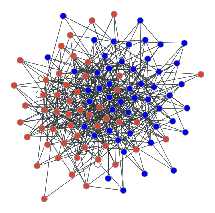
(a) Bicommunity partition

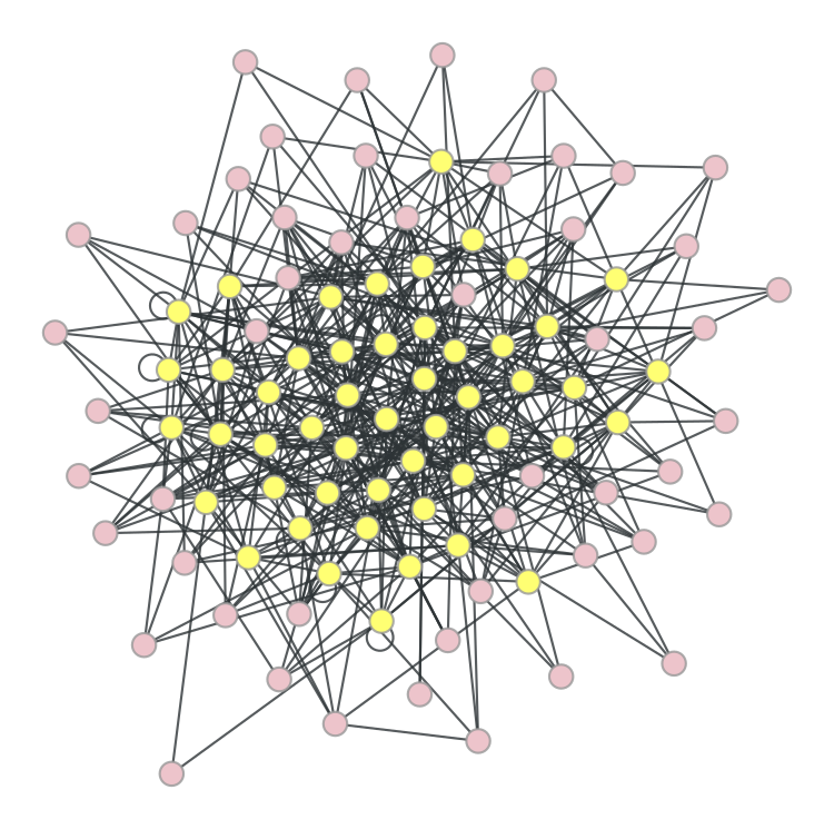
(b) Core-periphery partition

Figure 1: An example graph with nodes coloured according to their block memberships in the planted bicommunity partition (1(a)) and the planted core-periphery partition (1(b)).

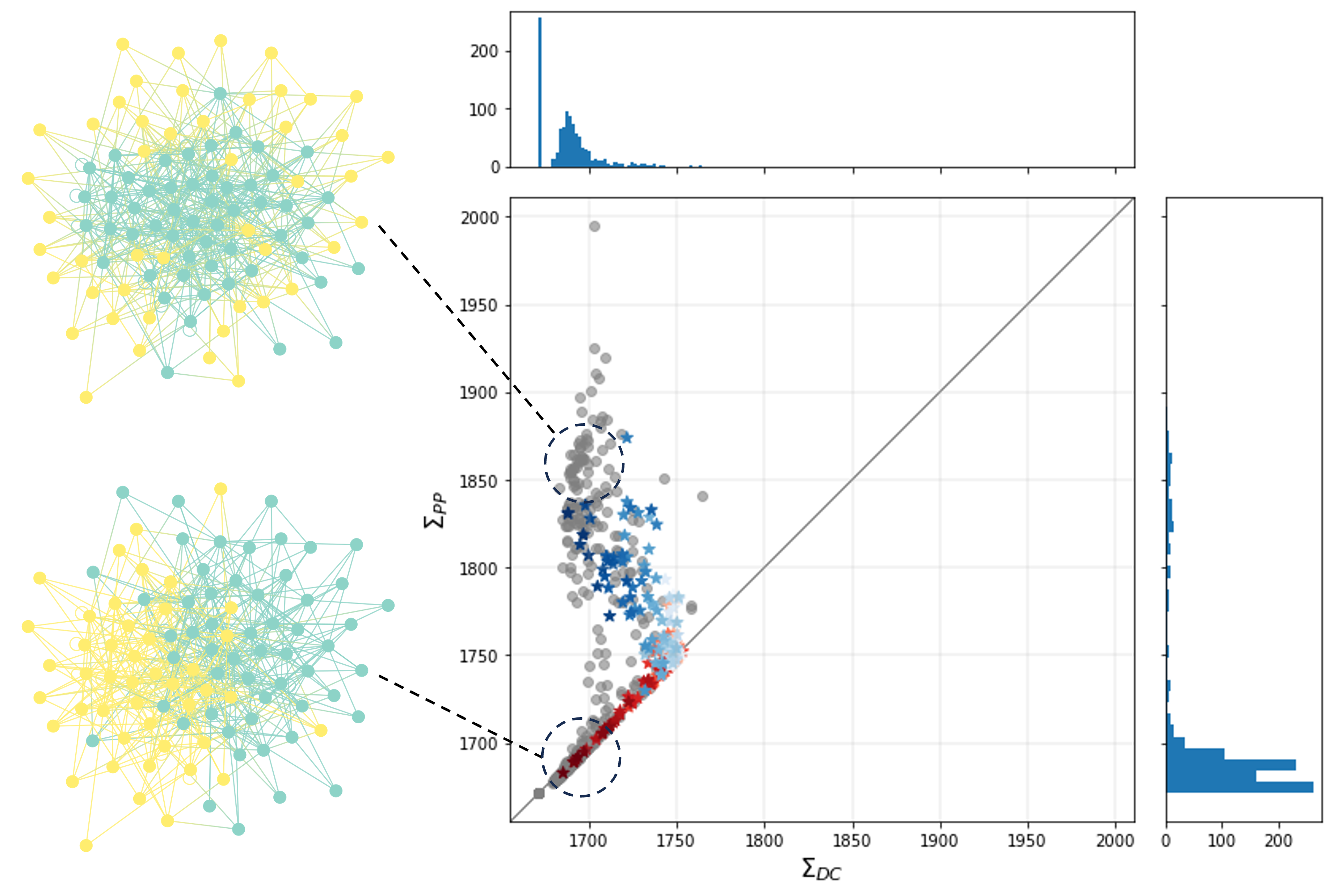
Figure 2: Description lengths under the DC and PP of the partitions sampled from DC (grey dots) and description lengths of the same network under DC and PP with metadata partitions (blue and red stars). The darker the colour of the stars representing the metadata partitions, the higher the correlation of the metadata labels with the respective planted structure. The network is visualised on the left-hand side, with nodes painted according to two of the sampled partitions. These two partitions are representative for clusters of partitions that have been grouped according to a partition similarity measure.

To demonstrate that this network does, in fact, exhibit a heterogeneous partition landscape, we fit an SBM to this network and sample from the posterior distribution by using the methods from the graph-tool library [73] (which has also been used to draw all network visualisations in this paper). In particular, we use the degree-corrected SBM variant (DC), which is meant to account for heterogeneous degree distributions within blocks [74]. The description lengths $\Sigma_{DC}$ of the network according to these partitions are plotted in grey dots on the x-axis in Figure 2. We also calculate the description lengths $\Sigma_{PP}$ of the network according to each partition under the planted partition SBM (PP), a variant of the model that assumes assortativity [22]; these are shown on the y-axis of the same figure. Note that, unsurprisingly, we find that $\Sigma_{PP}\leq\Sigma_{DC}$ for all partitions, since partitions were found by DC and corresponding description lengths were then calculated for the same partitions under PP. If we take a closer look at the partitions that we sampled, we find clusters of similar partitions, here marked by the dashed-line circles. We show representative partitions for each partition cluster in the two network visualisations on the left-hand side of the plot, in which nodes are painted according to block assignments. We clearly see a strong similarity between these inferred partitions and each of the two planted partitions in Figure 1 and we therefore conclude that we have successfully created a network with the desired diverse partition landscape. We also observe that for those inferred partitions that are similar to the planted bicommunity partition, the PP offers a similarly good encoding of the network as the DC, since $\Sigma_{PP}\approx\Sigma_{DC}$ for those partitions. In contrast, the description lengths of the network are considerably higher under the same partitions but according to PP. This illustrates that calculating the description length of a network under different models can help us probe its partition landscape.

In line with the objective of our measure, we use this example network to demonstrate that description length is a suitable tool to understand the relationship between metadata and network structure. For this purpose, we generate multiple sets of metadata in a way such that the labels align with the block structure of the network to varying degrees, similar to the related work in [7]. In fact – since we have planted two two-block partitions – we create multiple sets of metadata for both of them: one for BC, one for CP. For each of the planted block structures, we generate a set of metadata for each of a set of correlation values $\rho$, so that each node is labelled equal to the block assignment of the planted structure with probability $(1+\rho)/2$. We increase $\rho$ from $0$ to $1$ at steps of $0.01$, yielding $202$ sets of metadata in total, one being ‘bicommunity-like’ and one being ‘core-periphery-like’ to varying extents.

Intuitively, one way of measuring the relevance of a set of metadata to the network structure might be to calculate the partition similarity, either between the metadata partition and the ground truth partition (for synthetic networks, when this is available) or to inferred partitions in real networks. However, we will see later that in cases where the signal of the planted block structure is weak, the partition similarity approach fails. Instead, we quantify the relationship between metadata and structure by measuring how well a network would be encoded by an SBM if the metadata partition was the parameter of the model. In other words, how likely was an SBM – with the partition parameter being the metadata labels – responsible for the generation process of a given network. In order to quantify this, we first need to calculate the description length of the network under an SBM. In particular, we again do this under both the DC and the PP, and plot the resulting description length values, represented by the star symbols, alongside the description length values of the inferred partitions in Figure 2. The red stars represent the partitions that are correlated with the planted bicommunity structure, the blue stars represent those that are similar to the core-periphery structure, with darker colours depicting higher values of $\rho$. As expected, we observe that under the more general of the two models, the partitions with the highest values of $\rho$ have the lowest description length: the stronger the correlation of the metadata with the planted structure, the lower the description length, since the metadata partition is similar to the two ground truth partitions that were responsible for generating the network. The description lengths under the PP on the y-axis illustrate that additional to measuring the extent to which metadata is related to structure, we can also probe the type of structural arrangement: the bicommunity-like metadata are encoded as well under PP as under DC, indicating that assortativity was a prominent feature of the network generation process [22]. The core-periphery-like metadata, however, yield much higher description lengths under PP compared to DC, suggesting that – as we know is true – if we were to assume that this metadata was responsible for generating this network, assortativity was much less likely the prominent structure compared to some other more general structure.

We can see that for multiple sets of metadata with the same number of blocks and equal block sizes, using description length alone provides meaningful insight into the connection between metadata and structure – not just in terms of overall relevance but also in terms of probing types of arrangements. However, two features required for a measure that enables large-scale meta studies of collections of networks are not satisfied with this simple approach. Firstly, using raw description length values does not supply the necessary information to understand whether these measures are statistically significant; without having a point of reference, the description length of the network under a metadata partition does not tell us anything about whether this particular set of metadata describes the network better than a random partition of the network. Another issue is that raw description length values do not enable inter-network comparisons, the description length increases with growing network size and decreases with larger numbers of blocks and we thus cannot use it to compare networks of potentially different sizes, densities, block structures, and metadata partitions. We thus need to find a way to incorporate a notion of statistical significance into our measure and normalise it in a way that allows cross-network comparison.

Normalisation

To do so, we normalise our measure by the description length of the ‘best possible’ generative model that we can find. In an ideal scenario, the preferred approach would be to juxtapose the metadata partition under each model with the description length of the ‘true model’ thereby offering insight into how closely our models align with the actual generative process underlying the network. Regrettably, this is unattainable due to the inherent challenge of identifying the ‘true model’ [44]. Consequently, we instead compare each of our models with the best achievable model within our reach. To this end, we use the relevant functions from the graph-tool library [73] to separately fit each SBM variant $m$ to the network and infer the optimal partition under each model by minimising the description length. We then identify the description length of the overall optimal partition by finding the minimum out of the description lengths of the optimal partitions inferred by each SBM variant $m$, thus $\Sigma_{opt}=\min(\{\Sigma_{opt}^{m}\})$. Since $\Sigma_{opt}$ is the lowest possible description length associated with a partition inferred by any of the included SBM variants, it can be interpreted as the description length that is closest to the description length of the ‘true model’.

Statistical significance

To consider statistical significance in our measure, we take the description length of the network under an SBM with the observed metadata partition and compare it to the description length of the same network under an SBM with randomised metadata. This approach is inspired by the blockmodel entropy significance test (BESTest) [7], which produces a metadata p-value, i.e. the probability that a randomised version of the observed metadata describes the network better than (or equally well as) the observed metadata. The BESTest p-value is calculated by generating a large set of randomised metadata partitions (whereby the number of elements in each metadata category is fixed), computing the SBM entropy under each of the randomised partitions, and finally comparing the SBM entropy under the observed metadata partition to that of the randomised partitions. However, SBM entropy decreases for an increasing number of groups (see Section Description length) which greatly complicates direct comparison of metadata models (i.e. different metadata partitions and/or different SBM variants). Description length enables model selection and can thus be used to compare different sets of metadata for a given network.

Instead of calculating a p-value from distributions of description lengths, we identify the maximum significant description length $\Sigma_{*}$ of the randomised metadata. For a significance level of $\alpha=0.01$, $\Sigma_{*}$ is equal to the first percentile of the description length distribution of randomised metadata. The choice of $\alpha$ is, to some extent, arbitrary; here, we make the choice based on conventions in measuring statistical significance, according to which $\alpha=0.01$ denotes strong evidence against the null hypothesis, i.e. that the network is described equally well by randomised metadata. We emphasise that other choices can be made when our measure is used, as the required level of significance may depend on the specific context. In our measure, we take $\Sigma_{*}$ to be the maximum description length for which we would still consider the description length of the observed metadata to be relevant. To be exact, to calculate $\Sigma_{*}=\min(\{\Sigma_{*}^{m}\})$, where $\Sigma_{*}^{m}$ is the maximum significant description length for of the randomised metadata under SBM variant $m$.

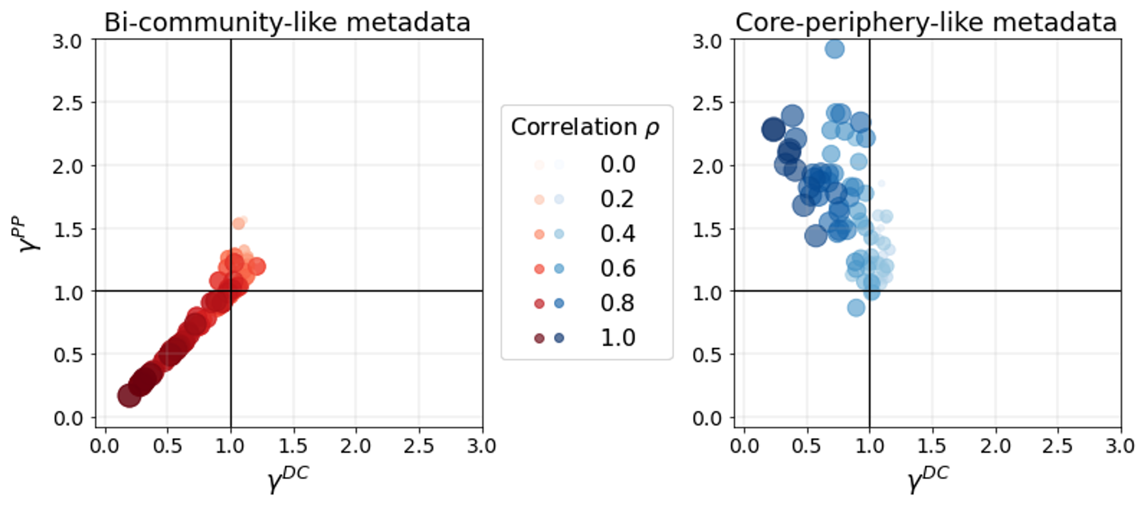
Figure 3: Metablox vectors $\boldsymbol{\gamma}$ of dimension (DC, PP) for a synthetic network with sets of metadata that are correlated with planted community structure (left) and core-periphery structure (right) to varying degrees.

Metadata block structure exploration (metablox)

Putting together these components in one measure, we finally arrive at our metablox pipeline which produces the vector $\boldsymbol{\gamma}_{d}$ for a metadata partition $d$, grounded in the notion of model selection outlined in Section Model selection and SMB variants. It can consist of as many elements as we include SBM variants to probe for different structural arrangements. Here, we will work with the two variants used in the motivating example, DC and PP as well as the non-degree-corrected SBM (NDC), thus $\boldsymbol{\gamma}$ is a vector with three elements. For a metadata partition $d$, the metablox vector $\boldsymbol{\gamma}_{d}$ thus consists of elements

$$\gamma^{m}_{d}=\frac{\Sigma_{d}^{m}-\Sigma_{opt}}{\Sigma_{*}-\Sigma_{opt}}$$ (4)

for each SBM variant $m$. $\Sigma_{d}^{m}$ is the description length of metadata partition $d$ under model $m$, $\Sigma_{*}$ is the maximum significant description length, and $\Sigma_{opt}$ is the description length of the optimal partition of the network. Recall that the difference in description length between two models is equal to the log of the posterior odds ratio of the two models. The numerator of $\gamma^{m}_{d}$ thus measures how much more likely the optimal partition is compared to the metadata partition under model $m$. Similarly, the denominator represents how much more likely the optimal partition is to the randomised metadata partitions under all models. The total measure is the former normalised by the latter.

With this definition, each element can then be interpreted as follows: for $\gamma^{m}_{d}\geq 1$ we say that this set of metadata is not relevant to the structure under model $m$, since more than $1\%$ of the randomised metadata partitions compress the network more efficiently than our observed metadata, under the given model. For $\gamma^{m}_{d}<1$, the metadata is relevant to the structure under the given model, and the closer $\gamma^{m}_{d}$ is to $0$, the stronger the relevance of the set of metadata to the block structure and the closer the structural arrangement of the metadata to the typical type of structure generated under the given model $m$. Another way of interpreting $\gamma^{m}_{d}$ is: relative to the best compression we can find, how efficient is the compression of the observed metadata $d$ under $m$ compared to partitioning the network by randomised versions of the metadata.

Note that for a network with some metadata partition $d$, $\gamma^{m_{1}}_{d}<\gamma^{m_{2}}_{d}$ merely tells us that, given the observed metadata, model $m_{1}$ provides a better explanation of the network than $m_{2}$. It does not necessarily mean that the block structure of our network as a whole is optimally explained by $m_{1}$. In fact, it is possible that SBM variant $m_{2}$ is the better model for the network as a whole, were we to calculate the log-evidence of each model (rather than comparing the description length of individual partitions) This is because $\Sigma_{opt}$ corresponds to the particular SBM variant that, as part of the inference procedure, yielded the partition with the lowest description length. For element $\gamma_{d}^{m}$ of $\boldsymbol{\gamma}$, this might not be the same as $m$.

In Figure 3, we show two dimensions of $\boldsymbol{\gamma}$ for our motivational network and its metadata. In particular, we calculate $\boldsymbol{\gamma}_{d}$ for each metadata partition $d$ out of all $202$ that we created for the network and we plot $\gamma_{d}^{DC}$ on the x-axis and $\gamma_{d}^{PP}$ on the y-axis, this time separately for the bicommunity-like metadata (left) and the core-periphery-like metadata (right). As before, darker colours correspond to a stronger correlation of the generated set of metadata with the planted block structure in each of the two coexisting partitions. By definition, and as can be observed in Figure 3, the elements of $\boldsymbol{\gamma}$ preserve the differences between the description lengths of the metadata partitions under the different variants of the measure. We also observe that for higher values of $\rho$, i.e. partitions that are more similar to the planted core-periphery partition, $\gamma_{PP}$ is higher than for partitions are less correlated to the planted structure. At the same time, $\gamma_{DC}$ is lower for partitions with high $\rho$ values. $\boldsymbol{\gamma}$ thus correctly identifies the partitions that are strongly related to the network structure when we use the more general of the SBM variants. On the other hand, partitions that have stronger correlation with the existing core-periphery block structure are less relevant under the PP model. $\boldsymbol{\gamma}$ therefore also identifies that these are the partitions that are least likely under the PP model.

We will see in Section Synthetic networks that $\boldsymbol{\gamma}$ is also mostly independent of network size, the number of metadata labels and the block structure. This means that it can be used across networks and thus as part of meta analyses.

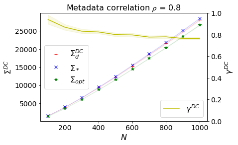
(a)

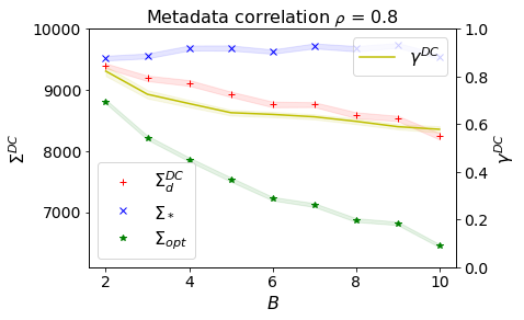
(b)

Figure 4: Optimal and metadata description lengths, and $\gamma^{DC}$ for increasing network size $N$ (left) and number of planted blocks $B$ (right).

Results

We demonstrate $\boldsymbol{\gamma}$ on a number of synthetic and real networks. Here, we include DC, NDC, and PP in the calculations for $\boldsymbol{\gamma}$. This means that $\boldsymbol{\gamma}$ is a vector of size three and – in this specific case – we also use the same three variants to calculate $\Sigma_{*}$ and $\Sigma_{opt}$. In many cases, it might be possible to come closer to identifying a more optimal partition (i.e. lower $\Sigma_{opt}$) by inferring the most likely partition for other SBM variants, such as the nested SBM [45], which has demonstrated to provide the best model fit in many cases [70]. It is straightforward to extend our measure to include as many SBM variants as desired in this calculation, but longer computation times must be expected, especially for large networks.

Synthetic networks

To demonstrate the suitability of the metablox measure to be used as part of comparative studies of networks of different sizes and topologies, we generate additional synthetic networks and run some robustness tests. Since the description length of a network increases with growing size $N$ and decreases with growing number of blocks $B$, we generate synthetic networks that allows us to test if $\boldsymbol{\gamma}$ is, in fact, independent of these factors. To check for the behaviour of metablox values for increasing network size, we increase $N$ from $N=100$ to $N=1000$ at steps of $100$, and generate $50$ networks for each $N$, all with expected degree $c=10$ and with planted bicommunity structure ($B=2$). In Figure 4(a), we plot the mean description lengths and metablox (plus $95\%$ confidence intervals) for each value of $N$. In particular, we plot all the individual components of $\gamma^{DC}_{d}$ as well as $\gamma^{DC}_{d}$ itself, where $d$ is a metadata partition that correlates with the planted bicommunity structure with probability $\rho=0.8$. In particular, the plot shows the description length of the metadata partition $\Sigma^{DC}_{d}$ (red plus symbols), the first percentile of the distribution of the description lengths of randomised metadata partitions $\Sigma_{*}$ (blue crosses) and the description length of the optimal partition $\Sigma_{opt}$ (green stars). Overall, we clearly see the intended normalising effect, as $\gamma^{DC}_{d}$ remains relatively stable for growing $N$. It appears that our measure is not perfectly independent of network size, as we observe a small decrease for $\gamma^{DC}_{d}$ as $N$ increases from the smallest values. While this bias should be considered when using our measure to compare networks of very different sizes and further analysis of the reasons for this effect should be explored in future work, the overall normalisation seems sufficient to use the measure on real networks.

To test the measure’s behaviour for varying numbers of blocks, we fix the network size at $N=400$ and leave all other parameters as above, increasing $B$ from $2$ to $10$, again generating $50$ networks at each step. Figure 4(b) shows that while the overall description lengths of metadata, randomised metadata and optimal partition decrease as $B$ increases, we again see that $\gamma^{DC}_{d}$ accounts for these differences to a large extent. As with the case of increasing $N$ the normalising effect is not perfect, but it seems sufficient to apply the measure in a comparative setting. Note that the same plots for the NDC component of the $\boldsymbol{\gamma}$ vector show an even stronger normalising effect; we briefly discuss this in Appendix B.

Real networks

We now show the metablox vector for multiple sets of real networks. The first one consists of the three Lazega law firm network [75]. In this set, there are three networks in which edges represents different types of connections between the employees of a corporate law firm (coworkers, friendship, and advice). For the employees, we include five sets of node attributes - their status in the firm, gender, one of three offices, which type of law they practice, and which law school they went to. The second set of networks contain data on four Twitter debates on political topics in the US. The original set of users on which these networks are based were collected by [76] and the ones used in this paper were recollected by [77]. The first three were collected between 2015 and 2016, and are based on conversations on abortion, Obamacare, and gun control. The fourth network represents conversations that happened on the day of the US presidential election in 2020. In all of these networks, the available node metadata reflects two categories of political orientation as either liberal or conservative, based on calculations made by the authors of [77] to estimate political opinion scores from shared URLs. Finally, we include a number of individual extra networks, accessed through the Netzschleuder network catalogue [79]. The first of these is the network of political blogs from 2004, in which nodes and edges represent blogs and hyperlinks between blogs respectively, and where blogs are given a conservative or liberal attribute [62]. The second one is the Zachary Karate Club friendship network, with edges representing friendship between the members of a karate club, and two sets of metadata representing a divide into the teachers and students and a divide into two arguing factions (often seen as the ground truth partition of this network), respectively [11]. The crime network [80] is a network of people involved in crimes in the 1990s in the US, where metadata refers to people’s roles in these crimes (suspects, victims, witnesses). Lastly, we include a facebook friendship ego network, in which node attributes represent the relationship context [81].

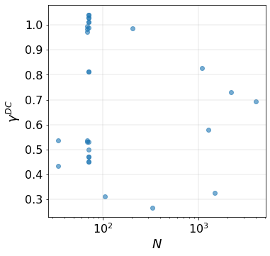
Figure 5: Metablox values under DC as a function of the number of nodes $N$ of all empirical networks in our collection.

We calculate the three-dimensional metablox vectors $\boldsymbol{\gamma}$ for each network-metadata pair. In Figure 5, we plot the DC component of $\boldsymbol{\gamma}$ for each of these pairs against the number of network nodes $N$, to show that there is no visible pattern that suggests a dependency of our measure on the network size.

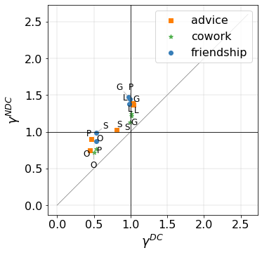
(a)

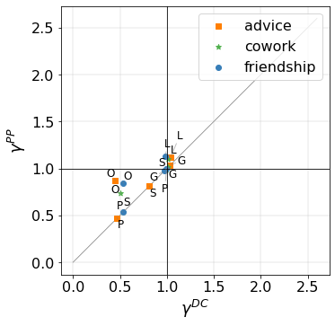
(b)

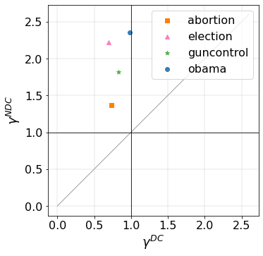
(c)

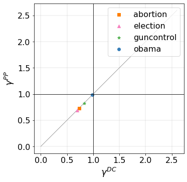
(d)

Figure 6: Metablox vectors for the law firm networks (top) and Twitter networks around US political debates (bottom), comparing DC to NDC (left) and to PP (right). The labels on the law firm figures represent the metadata partitions office (O), status (S), gender (G), law school (L), and practice (P).

Law firm networks

Figures 6(a) and 6(b) show the metablox vectors for the five metadata partitions of each of the three law firm networks; note that the numbers are also displayed in Table 1 in the appendix. On first sight, we can see some considerable variation with respect to the extent to which the metadata partitions are related to the network structure under each of the SBM variants. The law school that employees attended, for example is not related to the structure for any of the networks under any model, albeit barely significant under DC for the friendship network. Similarly, employees’ gender is not relevant to the edge generation process in the co-working and advice networks, and is somewhat relevant in the friendship network. The type of law practiced by an employee is not relevant to the formation of friendship ties but is strongly relevant in terms of co-working and advice ties. In these two networks, PP compresses this metadata partition equally well as DC, implying that assortativity was the prominent feature in the process. In the case of the friendship network, the status of employees is the attribute most strongly related to the edge formation, again similarly well explained by PP as by DC. Peel at al. [7] used the same networks to demonstrate both of their methods, which we outlined abo. In line with our results here, their methods indicate that all sets of metadata are relevant to the structure in at least one of the networks. However, they also concluded – using their second proposed method – that the law school metadata is more strongly related to the network structure of the friendship network than the office metadata. According to our metablox measure, both of these sets of metadata are relevant to the network under DC but the association is much stronger for the office metadata; we also find that under NDC, the office metadata is still relevant but the law school metadata is not. As mentioned previously, the methods proposed by the above authors can give insights into the relevance of the metadata to the structure and to the quality of the relationship by visually inspecting trajectories in the partition landscape, but they do not enable a direct quantification of the likely prominent structure. They also do not enable a direct comparison of different networks, something our measure is designed to do as demonstrated in the following paragraph.

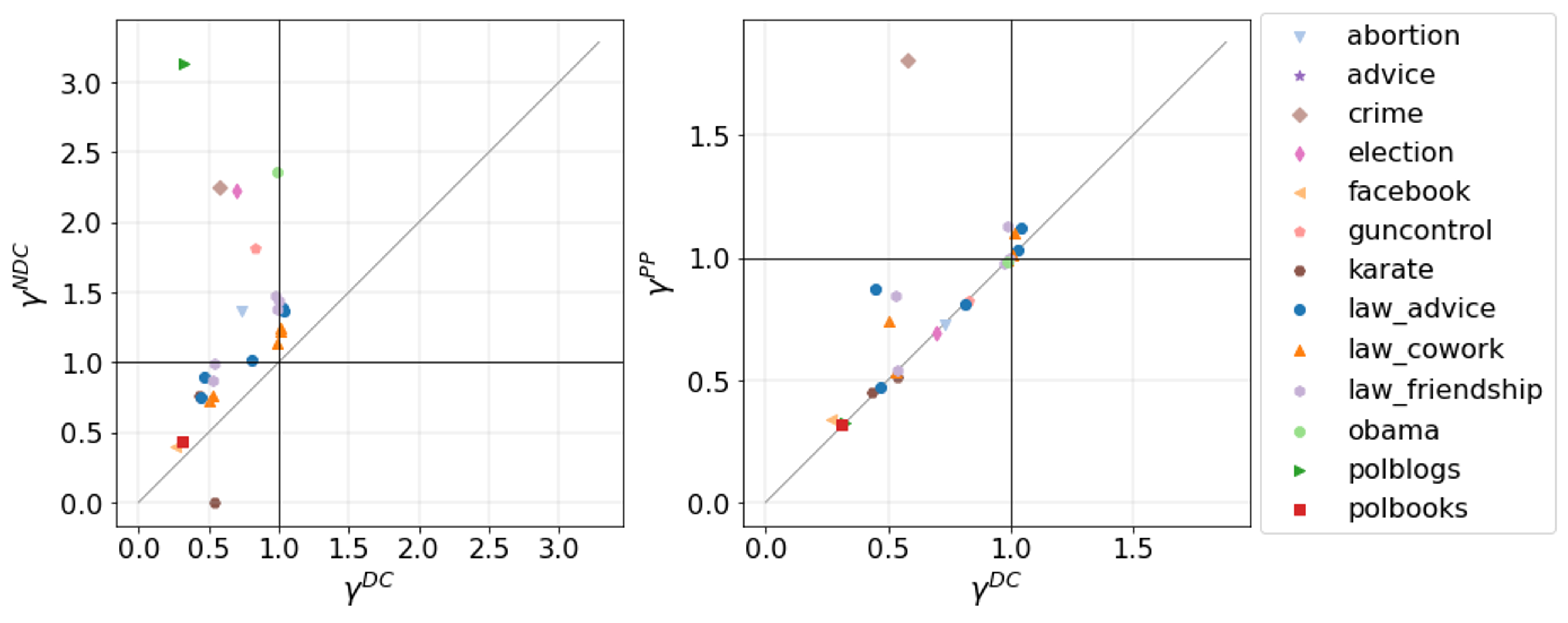
Figure 7: Metablox vectors for all of empirical networks, under DC and NDC (left) and under DC and PP (right).

Political Twitter networks

In Figures 6(c) and 6(d), we plot the metablox vectors for the Twitter interaction networks in which users debated political topics in a US context. We observe that in all four cases, the metadata partition into liberals and conservatives is relevant under DC and PP, but not under NDC. We can conclude that all metadata partitions were likely to be at least somewhat related to the data generating process and that assortativity is the prominent structural arrangement in all cases, albeit to varying degrees. Interestingly, the ordering of the four networks along the $x=y$ axis nearly corresponds with findings on polarisation levels in these networks, which classified the election network as the most polarised and the Obamacare network as the least polarised; only the abortion and gun control networks were reversed in the ordering [77]. Similar to our work, this particular polarisation measure also considers both network structure as well as a metadata dimension. However, their measure considers continuous node attributes – specifically political ideology on a continuous left-right scale – and specialises on measuring polarisation rather than the more general approach we take here. So although our measure has a different purpose, it is interesting to see that it might be able to pick up specific network properties (such as polarisation or fragmentation) while also being general enough to enable broader comparisons.

Cross-network comparison

Finally, we show $\gamma$ for all empirical networks (including the extra networks mentioned at the beginning of Section Real networks) combined in one plot (Figure 7), to illustrate that our measure serves not only for a comparison between multiple metadata partitions of one network, or between multiple networks of the same type, but also of collections of networks that represent different data sources altogether. This facilitates a quick identification of networks which stand out in the way in which a particular metadata partition is related to the structure. In this case, for example, we can see that one of the metadata partitions of the Karate club network (it happens to be the teacher-student partition) is better explained by NDC than by DC. We can also find the network for which the metadata is closest related to the structure (the facebook ego network), or the one for which a particular SBM is a particularly unlikely explanation of the structure under the metadata partition.

Discussion

In this paper, we have introduced a novel measure for probing the relationship between network metadata and its structural organization. Our metablox pipeline, which produces the vector $\boldsymbol{\gamma}$, is designed to provide insights into the relevance of metadata to network structure and the likely structural arrangement within the network. We have applied this measure to both synthetic and real-world networks to demonstrate its utility in various scenarios.

Our analysis of synthetic networks confirmed that $\boldsymbol{\gamma}$ remains relatively constant across networks of different sizes and numbers of planted blocks, indicating its robustness and suitability for comparative studies. This property allows us to use $\boldsymbol{\gamma}$ as a tool for cross-network comparisons, enabling us to assess the relevance of metadata and the likely structural arrangement in diverse network data sources.

We have further applied the metablox measure to a collection of real-world networks, including the Lazega law firm networks, Twitter debates, and various other networks. The results reveal variations in the relevance of metadata partitions and the likely structural arrangement, providing valuable insights into the underlying dynamics of these networks. For instance, we observed that metadata partitions related to political orientation in the Twitter debate networks were relevant under degree-corrected (DC) and planted partition (PP) stochastic block models but not under non-degree-corrected (NDC) models. This suggests that assortativity is a prominent feature in these networks, that have been shown to exhibit varying degrees of polarisation [82, 77]. Our measure allows for a comprehensive cross-network comparison, enabling researchers to quickly identify networks where specific metadata partitions are closely related to structure or where certain structural arrangements are unlikely under the metadata.

In terms of future work, there are several directions in which this measure can be extended and applied to address a broader range of research questions and network types. One potential extension of $\boldsymbol{\gamma}$ involves incorporating additional dimensions to capture various structural patterns in networks. Currently, we focus on degree-corrected (DC), non-degree-corrected (NDC), and planted partition (PP) stochastic block models. However, networks often exhibit more complex structural arrangements beyond these models. Future work could explore the integration of other SBM variants that are tailored to specific structural motifs, such as core-periphery structures, bipartite structures or nested patterns. The current measure has been implemented for undirected simple graphs, but extensions to more complex network structures such as directed graphs and multigraphs are straightforward and should also be considered as part of future research.

Our measure has the potential to serve as a tool for conducting large-scale comparisons of collections of network-metadata pairs, another promising avenue for further research. This sort of analysis is conceivable for networks coming from a variety of research fields – as long as categorical node metadata is available. Obvious examples for possible studies in this regard are different types of social networks, for which metadata may include a range of demographics or affiliations. In this scenario, researchers could examine the relevance of different attributes (e.g., age, gender, interests) to the formation of social ties and identify common structural patterns across networks. Another possible subfield which may benefit from this type of measure is that of biological networks (such as gene regulatory networks, protein-protein interaction networks, and ecological networks). These types of networks frequently incorporate categorical metadata related to genes, proteins, or species and researchers could thus calculate metablox vectors to assess how these metadata attributes influence the network’s structural organization. This approach can provide insights into the functional relationships in biological systems. Networks in the economic and financial domains, such as trade networks, supply chains, and stock market networks, also often involve categorical metadata related to industries, sectors, or companies. $\boldsymbol{\gamma}$ can be employed to investigate the degree to which this metadata is associated with network structures, revealing potential patterns and dependencies in these complex systems. Lastly, another interesting field for using our measure could be networks in science of science, where networks represent collaborations and knowledge flows, and metadata may include fields of scientific research. Here researchers could employ $\boldsymbol{\gamma}$ to identify commonalities and differences in how common research areas influence edge formation.

Appendix A Description length calculations

The description length calculations for NDC and DC are based on the work in [69, 38], that for PP comes from [22]. We start with the elements of the joint distribution of NDC,

$$P(A,e,b)=P(A|e,b)P(e|b)P(b)$$ (5)

The model likelihood of NDC is given by

$$P(A|e,b)=\frac{\prod_{r<s}e_{rs}!\prod_{r}e_{rr}!!}{\prod_{r}n_{r}^{e_{r}}\prod_{i<j}A_{ij}!\prod_{i}A_{ii}!!}$$ (6)

We use a uniform prior for the block matrix $e_{rs}$, based on the total possible number of symmetric block matrices given $B$, with the constraint that the sum of all elements must equal $2E$:

$$P(e|b)=\left(\!\!{B(B+1)/2\choose E}\!\!\right)^{-1}$$ (7)

The prior on the partition is defined as

$$P(b) =P(b|n)P(n|B)P(B)$$ (8)

$$=\frac{\sum_{r}n_{r}!}{N!}{N-1\choose B-1}^{-1}\frac{1}{N}.$$

Here, $P(B)$ and $P(n|B)$ are hyperpriors on the number of blocks $B$ and on the block sizes $n_{r}$ respectively, which we include in order to be as parsimonious as possible about these parameters. In the case of DC, the model likelihood includes terms for the degree sequence $k$, so that:

$$P(A|e,k,b)=\frac{\prod_{r<s}e_{rs}!\prod_{r}e_{rr}!!\prod_{i}k_{i}!}{\prod_{r}e_{r}!\prod_{i<j}A_{ij}!\prod_{i}A_{ii}!!}$$ (9)

In the case of DC, we also need to include a prior on the degree sequence $k$, for which we use

$$P(k|e,b)=\prod_{r}\frac{\prod_{k}\eta_{k}^{r}!}{n_{r}!}\prod_{r}q(e_{r},n_{r})^{-1}.$$ (10)

where $\eta$ denotes the number of degree-$k$ nodes in group $r$ and $q(x,y)$ is the number of times an integer $x$ can be partitioned into a maximum of $y$ parts [38].

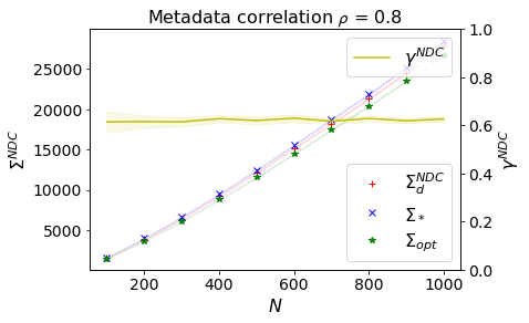
(a)

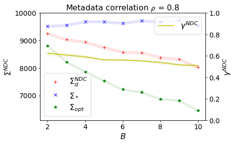
(b)

Figure 8: Optimal and metadata description lengths, and $\gamma^{NDC}$ for increasing network size $N$ (left) and number of planted blocks $B$ (right).

For PP, the prior on the block matrix needs to be defined differently, to encode the constraint that is put on the structural arrangement [71]. In fact, Zhang and Peixoto [22] proposed two different versions of this probability: one which assumes that uniform expected number of edges within each community and one that allows the number of expected edges to vary across communities (non-uniform). Here, we give the formulation for both versions, since in our analysis, we use the uniform version in the case of synthetic networks (since they are generated with equal size blocks) and the non-uniform version in the analysis of the metablox vector on real networks. The uniform version of the prior on the edge counts in PP is described by

$$P(e|e_{in},e_{out}|b)P(e_{in},e_{out}|E,b),$$ (11)

with

$$P(e|e_{in},e_{out}|b)=\frac{e_{in}!e_{out}!}{B^{e_{out}}\sum_{r}(e_{rr}/2)!{B\choose 2}^{e_{out}}\sum_{r<s}e_{rs}!},$$ (12)

at which we arrive by multiplying one uniform multinomial distributions for the elements of the block matrix that correspond to the within-block edge counts and one for those that correspond to the between-block edge counts, given $e_{in}$ and $e_{out}$. The second part is then the hyperprior on $e_{in}$ and $e_{out}$:

$$P(e_{in},e_{out}|E,b)=\left(\frac{1}{E+1}\right)^{1-\delta_{B,1}}$$ (13)

For the non-uniform version, the prior is also made up of two probabilities

$$P(e|\{e_{rr}\},e_{out},b)P(\{e_{rr}\},e_{out}|b,E)$$ (14)

where

$$P(e|\{e_{rr}\},e_{out},b)=\frac{e_{out}!}{{B\choose 2}^{e_{out}}\sum_{r<s}e_{rs}!}$$ (15)

corresponds to a uniform multinomial distribution for the off-diagonal elements of the block matrix given $e_{out}$. The second component is made out of a uniform distribution over all possible values $e_{in}$ from $E$, and a uniform distribution over all ways of choosing the set of diagonal block matrix values $\{e_{rr}\}$, given $e_{in}$:

$$P(\{e_{rr}\},e_{out}|b,E) =P(\{e_{rr}\}|e_{in},b)P(e_{in}|E,b)$$ (16)

$$={B+e_{in}-1\choose e_{in}}^{-1}\left(\frac{1}{E+1}\right)^{1-\delta_{B,1}}.$$

Appendix B Robustness tests for non-degree-corrected variant

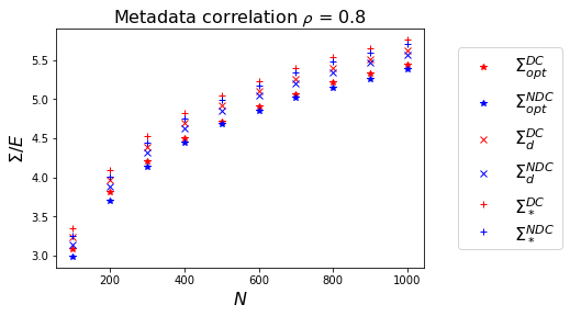
(a)

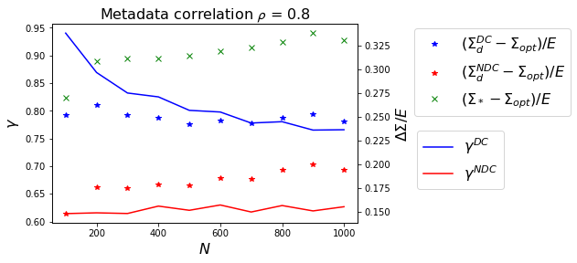
(b)

Figure 9: Top: All individual description length components of $\gamma^{DC}$ and $\gamma^{NDC}$ (mean over all generated networks) for varying network sizes $N$: metadata description length, description length of optimal partition, maximum significant description length of randomised metadata. Bottom: $\gamma^{DC}$ and $\gamma^{NDC}$, and the numerator and denominator of each of them (normalised by number of edges), for increasing network sizes $N$.

In Figure 8, we plot the description lengths of the optimal partition, the maximum significant description length of the randomised metadata, and the metadata description length, as well as $\gamma_{NDC}$. Unlike the DC case, for which there is a small decrease in $\gamma_{DC}$ for increasing network size and number of blocks, $\gamma^{NDC}$ appears entirely independent of $N$ and $B$. One possible explanation for the small decreases in $\gamma^{DC}$ for increasing $N$ and $B$ and for the larger robustness for $\gamma^{NDC}$ could be related to the generative processes responsible for creating the networks. The synthetic networks in these simulations were generated with the planted partition model [72] – using a traditional SBM to create networks with unambiguous block structure without considering node degrees. This means that (i) these networks’ partition landscapes should be relatively ‘unimodal’ unlike the motivational network above, and that (ii) we expect NDC to have the best model fit overall. Indeed, we find that in this particular case $\Sigma_{opt}$ is the description length of a partition inferred from NDC for all $N$, and that the maximum significant description length of the randomised metadata $\Sigma_{*}$ also comes from NDC in all cases (both can be seen in Figure 9(a)). We can see the possible effect of this in Figure 9(b), where it becomes clear that the numerator and denominator of $\gamma^{NDC}$ increase at a very similar rate, while the numerator of $\gamma^{DC}$ stays flat with growing $N$. It thus seems likely that the difference in robustness with respect to $N$ is due to the fact that for $\gamma^{NDC}$, all components are taken from the same variant (NDC), whereas for $\gamma^{DC}$, the $\Sigma^{DC}_{d}$ component is compared to description lengths from a different variant. A more thorough exploration of this is required and should be the object of study in future work.

Table 1: Metablox values for the three law firm networks and the five sets of node attributes.

Network	Metadata	$\gamma^{DC}$	$\gamma^{NDC}$	$\gamma^{PP}$
friendship	Status	0.54	0.99	0.54
friendship	Gender	0.97	1.47	0.97
friendship	Office	0.53	0.88	0.85
friendship	Practice	1.00	1.44	1.00
friendship	LawSchool	0.98	1.38	1.13
cowork	Status	0.99	1.13	0.99
cowork	Gender	1.01	1.22	1.01
cowork	Office	0.50	0.72	0.74
cowork	Practice	0.53	0.77	0.53
cowork	LawSchool	1.01	1.24	1.10
advice	Status	0.81	1.02	0.81
advice	Gender	1.03	1.39	1.03
advice	Office	0.45	0.75	0.87
advice	Practice	0.47	0.90	0.47
advice	LawSchool	1.04	1.36	1.12

References

- Lorrain and White [1971] Francois Lorrain and Harrison C White. Structural equivalence of individuals in social networks. The Journal of mathematical sociology, 1(1):49–80, 1971.
- White et al. [1976] Harrison C White, Scott A Boorman, and Ronald L Breiger. Social structure from multiple networks. i. blockmodels of roles and positions. American journal of sociology, 81(4):730–780, 1976.
- Holland et al. [1983] Paul W. Holland, Kathryn Blackmond Laskey, and Samuel Leinhardt. Stochastic blockmodels: First steps. Social Networks, 5(2):109–137, June 1983. ISSN 03788733. doi:10.1016/0378-8733(83)90021-7.
- Karrer and Newman [2011] Brian Karrer and M. E. J. Newman. Stochastic blockmodels and community structure in networks. Physical Review E, 83(1):016107, January 2011. ISSN 1539-3755, 1550-2376. doi:10.1103/PhysRevE.83.016107.
- Newman and Clauset [2016] Mark EJ Newman and Aaron Clauset. Structure and inference in annotated networks. Nature communications, 7(1):1–11, 2016.
- Hric et al. [2016] Darko Hric, Tiago P. Peixoto, and Santo Fortunato. Network Structure, Metadata, and the Prediction of Missing Nodes and Annotations. Physical Review X, 6(3):031038, September 2016. ISSN 2160-3308. doi:10.1103/PhysRevX.6.031038.
- Peel et al. [2017] Leto Peel, Daniel B Larremore, and Aaron Clauset. The ground truth about metadata and community detection in networks. Science Advances, 3(5):e1602548, 2017. doi:10.1126/sciadv.1602548.
- Conover et al. [2011] Michael Conover, Jacob Ratkiewicz, Matthew Francisco, Bruno Gonçalves, Filippo Menczer, and Alessandro Flammini. Political polarization on twitter. In Proceedings of the International Aaai Conference on Web and Social Media, volume 5, pages 89–96, 2011.
- Barberá et al. [2015] Pablo Barberá, John T. Jost, Jonathan Nagler, Joshua A. Tucker, and Richard Bonneau. Tweeting From Left to Right: Is Online Political Communication More Than an Echo Chamber? Psychological Science, 26(10):1531–1542, October 2015. ISSN 0956-7976. doi:10.1177/0956797615594620.
- Small and Griffith [1974] Henry Small and Belver C Griffith. The structure of scientific literatures i: Identifying and graphing specialties. Science studies, 4(1):17–40, 1974.
- Zachary [1977] Wayne W. Zachary. An Information Flow Model for Conflict and Fission in Small Groups. Journal of Anthropological Research, 33(4):452–473, December 1977. ISSN 0091-7710, 2153-3806. doi:10.1086/jar.33.4.3629752.
- Traud et al. [2012] Amanda L Traud, Peter J Mucha, and Mason A Porter. Social structure of facebook networks. Physica A: Statistical Mechanics and its Applications, 391(16):4165–4180, 2012.
- Yang and Leskovec [2012] Jaewon Yang and Jure Leskovec. Defining and evaluating network communities based on ground-truth. In Proceedings of the ACM SIGKDD Workshop on Mining Data Semantics, pages 1–8, 2012.
- Chakrabort et al. [2013] Tanmoy Chakrabort, Sandipan Sikdar, Vihar Tammana, Niloy Ganguly, and Animesh Mukherjee. Computer science fields as ground-truth communities: Their impact, rise and fall. In Proceedings of the 2013 IEEE/ACM International Conference on Advances in Social Networks Analysis and Mining, pages 426–433, 2013.
- Yang et al. [2013] Jaewon Yang, Julian McAuley, and Jure Leskovec. Community Detection in Networks with Node Attributes. In 2013 IEEE 13th International Conference on Data Mining, pages 1151–1156, December 2013. doi:10.1109/ICDM.2013.167.
- Bothorel et al. [2015] Cecile Bothorel, Juan David Cruz, Matteo Magnani, and Barbora Micenková. Clustering attributed graphs: Models, measures and methods. Network Science, 3(3):408–444, September 2015. ISSN 2050-1242, 2050-1250. doi:10.1017/nws.2015.9.
- Binkiewicz et al. [2017] Norbert Binkiewicz, Joshua T Vogelstein, and Karl Rohe. Covariate-assisted spectral clustering. Biometrika, 104(2):361–377, 2017.
- Peixoto [2021] Tiago P. Peixoto. Revealing Consensus and Dissensus between Network Partitions. Physical Review X, 11(2):021003, April 2021. ISSN 2160-3308. doi:10.1103/PhysRevX.11.021003.
- Mangold and Roth [2023] Lena Mangold and Camille Roth. Generative models for two-ground-truth partitions in networks. Physical Review E, 108(5):054308, November 2023. doi:10.1103/PhysRevE.108.054308.
- Grünwald [2007] Peter D Grünwald. The minimum description length principle. MIT press, 2007.
- Nowicki and Snijders [2001] Krzysztof Nowicki and Tom A B Snijders. Estimation and prediction for stochastic blockstructures. Journal of the American statistical association, 96(455):1077–1087, 2001.
- Zhang and Peixoto [2020] Lizhi Zhang and Tiago P. Peixoto. Statistical inference of assortative community structures. Physical Review Research, 2(4):043271, November 2020. ISSN 2643-1564. doi:10.1103/PhysRevResearch.2.043271.
- Coleman et al. [1964] James Samuel Coleman et al. Introduction to mathematical sociology. Introduction to mathematical sociology., 1964.
- Wasserman and Faust [1994] Stanley Wasserman and Katherine Faust. Social network analysis: Methods and applications. Cambridge university press, 1994.
- Luce and Perry [1949] R. Duncan Luce and Albert D. Perry. A method of matrix analysis of group structure. Psychometrika, 14(2):95–116, 1949. doi:10.1007/BF02289146.
- Alba [1973] Richard D. Alba. A graph-theoretic definition of a sociometric clique. Journal of Mathematical Sociology, 3(1):113–126, 1973. doi:10.1080/0022250X.1973.9989826.
- Mokken et al. [1979] Robert J Mokken et al. Cliques, clubs and clans. Quality & Quantity, 13(2):161–173, 1979.
- Kadushin [1968] Charles Kadushin. Power, influence and social circles: A new methodology for studying opinion makers. American Sociological Review, pages 685–699, 1968.
- Mohr and Duquenne [1997] John W Mohr and Vincent Duquenne. The duality of culture and practice: Poverty relief in new york city, 1888-1917. Theory and society, 26(2/3):305–356, 1997.
- Mullins et al. [1977] Nicholas C Mullins, Lowell L Hargens, Pamela K Hecht, and Edward L Kick. The group structure of cocitation clusters: A comparative study. American sociological review, pages 552–562, 1977.
- Borgatti and Everett [2000] Stephen P Borgatti and Martin G Everett. Models of core/periphery structures. Social networks, 21(4):375–395, 2000.
- Colizza et al. [2006] Vittoria Colizza, Alessandro Flammini, M Angeles Serrano, and Alessandro Vespignani. Detecting rich-club ordering in complex networks. Nature physics, 2(2):110–115, 2006.
- Dorogovtsev et al. [2006] Sergey N Dorogovtsev, Alexander V Goltsev, and Jose Ferreira F Mendes. K-core organization of complex networks. Physical review letters, 96(4):040601, 2006.
- White and Reitz [1983] Douglas R White and Karl P Reitz. Graph and semigroup homomorphisms on networks of relations. Social Networks, 5(2):193–234, 1983.
- Everett and Borgatti [1994] Martin G Everett and Stephen P Borgatti. Regular equivalence: General theory. Journal of mathematical sociology, 19(1):29–52, 1994.
- Fortunato [2010] Santo Fortunato. Community detection in graphs. Physics Reports, 486(3):75–174, February 2010. ISSN 0370-1573. doi:10.1016/j.physrep.2009.11.002.
- Rosvall et al. [2019] Martin Rosvall, Jean-Charles Delvenne, Michael T. Schaub, and Renaud Lambiotte. Different Approaches to Community Detection. In Advances in Network Clustering and Blockmodeling, chapter 4, pages 105–119. John Wiley & Sons, Ltd, 2019. ISBN 978-1-119-48329-8. doi:10.1002/9781119483298.ch4.
- Peixoto [2017] Tiago P. Peixoto. Nonparametric Bayesian inference of the microcanonical stochastic block model. Physical Review E, 95(1):012317, January 2017. ISSN 2470-0045, 2470-0053. doi:10.1103/PhysRevE.95.012317.
- Peixoto [2014a] Tiago P Peixoto. Efficient monte carlo and greedy heuristic for the inference of stochastic block models. Physical Review E, 89(1):012804, 2014a.
- Newman [2004] Mark EJ Newman. Fast algorithm for detecting community structure in networks. Physical review E, 69(6):066133, 2004.
- Fortunato and Barthelemy [2007] Santo Fortunato and Marc Barthelemy. Resolution limit in community detection. Proceedings of the national academy of sciences, 104(1):36–41, 2007.
- Good et al. [2010] Benjamin H. Good, Yves-Alexandre de Montjoye, and Aaron Clauset. Performance of modularity maximization in practical contexts. Physical Review E, 81(4):046106, April 2010. ISSN 1539-3755, 1550-2376. doi:10.1103/PhysRevE.81.046106.
- Guimera et al. [2004] Roger Guimera, Marta Sales-Pardo, and Luís A Nunes Amaral. Modularity from fluctuations in random graphs and complex networks. Physical Review E, 70(2):025101, 2004.
- Peixoto [2022] Tiago P. Peixoto. Descriptive vs. inferential community detection: Pitfalls, myths and half-truths. arXiv:2112.00183 [physics, stat], January 2022.
- Peixoto [2014b] Tiago P. Peixoto. Hierarchical block structures and high-resolution model selection in large networks. Physical Review X, 4(1):011047, 2014b. doi:10.1103/PhysRevX.4.011047.
- Airoldi et al. [2008] Edoardo M Airoldi, David M Blei, Stephen E Fienberg, and Eric P Xing. Mixed Membership Stochastic Blockmodels. Advances in neural information processing systems, 21, 2008.
- Godoy-Lorite et al. [2016] Antonia Godoy-Lorite, Roger Guimerà, Cristopher Moore, and Marta Sales-Pardo. Accurate and scalable social recommendation using mixed-membership stochastic block models. Proceedings of the National Academy of Sciences, 113(50):14207–14212, December 2016. doi:10.1073/pnas.1606316113.
- Peixoto [2015a] Tiago P. Peixoto. Model Selection and Hypothesis Testing for Large-Scale Network Models with Overlapping Groups. Physical Review X, 5(1):011033, March 2015a. ISSN 2160-3308. doi:10.1103/PhysRevX.5.011033.
- Peixoto [2015b] Tiago P. Peixoto. Inferring the mesoscale structure of layered, edge-valued, and time-varying networks. Physical Review E, 92(4):042807, October 2015b. ISSN 1539-3755, 1550-2376. doi:10.1103/PhysRevE.92.042807.
- Tarrés-Deulofeu et al. [2019] Marc Tarrés-Deulofeu, Antonia Godoy-Lorite, Roger Guimera, and Marta Sales-Pardo. Tensorial and bipartite block models for link prediction in layered networks and temporal networks. Physical Review E, 99(3):032307, 2019.
- Yen and Larremore [2020] Tzu-Chi Yen and Daniel B. Larremore. Community Detection in Bipartite Networks with Stochastic Blockmodels. Physical Review E, 102(3):032309, September 2020. ISSN 2470-0045, 2470-0053. doi:10.1103/PhysRevE.102.032309.
- Zhang et al. [2015] Xiao Zhang, Travis Martin, and M. E. J. Newman. Identification of core-periphery structure in networks. Physical Review E, 91(3):032803, March 2015. ISSN 1539-3755, 1550-2376. doi:10.1103/PhysRevE.91.032803.
- Gallagher et al. [2021] Ryan J. Gallagher, Jean-Gabriel Young, and Brooke Foucault Welles. A clarified typology of core-periphery structure in networks. Science Advances, 7(12):eabc9800, 2021. doi:10.1126/sciadv.abc9800.
- Peixoto [2019] Tiago P. Peixoto. Bayesian stochastic blockmodeling. arXiv:1705.10225 [cond-mat, physics:physics, stat], pages 289–332, November 2019. doi:10.1002/9781119483298.ch11.
- Abbe [2017] Emmanuel Abbe. Community detection and stochastic block models: Recent developments. The Journal of Machine Learning Research, 18(1):6446–6531, 2017.
- Girvan and Newman [2002] Michelle Girvan and Mark EJ Newman. Community structure in social and biological networks. Proceedings of the national academy of sciences, 99(12):7821–7826, 2002. doi:10.1073/pnas.122653799.
- Danon et al. [2005] Leon Danon, Albert Diaz-Guilera, Jordi Duch, and Alex Arenas. Comparing community structure identification. Journal of statistical mechanics: Theory and experiment, 2005(09):P09008, 2005.
- Fortunato and Hric [2016] Santo Fortunato and Darko Hric. Community detection in networks: A user guide. Physics Reports, 659:1–44, November 2016. ISSN 03701573. doi:10.1016/j.physrep.2016.09.002.
- Lancichinetti and Fortunato [2009] Andrea Lancichinetti and Santo Fortunato. Community detection algorithms: A comparative analysis. Physical Review E, 80(5):056117, November 2009. ISSN 1539-3755, 1550-2376. doi:10.1103/PhysRevE.80.056117.
- Lancichinetti et al. [2008] Andrea Lancichinetti, Santo Fortunato, and Filippo Radicchi. Benchmark graphs for testing community detection algorithms. Physical review E, 78(4):046110, 2008.
- Chunaev [2020] Petr Chunaev. Community detection in node-attributed social networks: a survey. Computer Science Review, 37:100286, 2020.
- Adamic and Glance [2005] Lada A Adamic and Natalie Glance. The political blogosphere and the 2004 us election: divided they blog. In Proceedings of the 3rd international workshop on Link discovery, pages 36–43, 2005.
- Himelboim et al. [2013] Itai Himelboim, Stephen McCreery, and Marc Smith. Birds of a feather tweet together: Integrating network and content analyses to examine cross-ideology exposure on Twitter. Journal of computer-mediated communication, 18(2):154–174, 2013.
- Hric et al. [2014] Darko Hric, Richard K Darst, and Santo Fortunato. Community detection in networks: Structural communities versus ground truth. Physical Review E, 90(6):062805, 2014.
- Newman [2003] Mark EJ Newman. Mixing patterns in networks. Physical review E, 67(2):026126, 2003.
- Newman and Girvan [2004] M. E. J. Newman and M. Girvan. Finding and evaluating community structure in networks. Physical Review E, 69(2):026113, February 2004. ISSN 1539-3755, 1550-2376. doi:10.1103/PhysRevE.69.026113.
- Peixoto [2013] Tiago P. Peixoto. Parsimonious module inference in large networks. Physical review letters, 110(14):148701, 2013.
- Bianconi [2009] Ginestra Bianconi. Entropy of network ensembles. Physical Review E, 79(3):036114, March 2009. ISSN 1539-3755, 1550-2376. doi:10.1103/PhysRevE.79.036114.
- Peixoto [2012] Tiago P. Peixoto. Entropy of stochastic blockmodel ensembles. Physical Review E, 85(5):056122, May 2012. ISSN 1539-3755, 1550-2376. doi:10.1103/PhysRevE.85.056122.
- Peixoto and Kirkley [2023] Tiago P. Peixoto and Alec Kirkley. Implicit models, latent compression, intrinsic biases, and cheap lunches in community detection, March 2023.
- Young et al. [2018] Jean-Gabriel Young, Guillaume St-Onge, Patrick Desrosiers, and Louis J. Dubé. Universality of the stochastic block model. Physical Review E, 98(3):032309, September 2018. ISSN 2470-0045, 2470-0053. doi:10.1103/PhysRevE.98.032309.
- Condon and Karp [2001] Anne Condon and Richard M. Karp. Algorithms for graph partitioning on the planted partition model. Random Structures & Algorithms, 18(2):116–140, 2001. ISSN 1098-2418. doi:10.1002/1098-2418(200103)18:2<116::AID-RSA1001>3.0.CO;2-2.
- Peixoto [2014c] Tiago P. Peixoto. The graph-tool python library. figshare, 2014c. doi:10.6084/m9.figshare.1164194. URL http://figshare.com/articles/graph_tool/1164194.
- Karrer et al. [2008] Brian Karrer, Elizaveta Levina, and Mark EJ Newman. Robustness of community structure in networks. Physical review E, 77(4):046119, 2008.
- Lazega [2001] Emmanuel Lazega. The collegial phenomenon: The social mechanisms of cooperation among peers in a corporate law partnership. Oxford University Press, USA, 2001.
- Garimella et al. [2018a] Kiran Garimella, Gianmarco De Francisci Morales, Aristides Gionis, and Michael Mathioudakis. Political discourse on social media: Echo chambers, gatekeepers, and the price of bipartisanship. In Proceedings of the 2018 world wide web conference, pages 913–922, 2018a.
- Hohmann et al. [2023] Marilena Hohmann, Karel Devriendt, and Michele Coscia. Quantifying ideological polarization on a network using generalized Euclidean distance. Science Advances, 9(9):eabq2044, March 2023. doi:10.1126/sciadv.abq2044.
- Cinelli et al. [2021] Matteo Cinelli, Gianmarco De Francisci Morales, Alessandro Galeazzi, Walter Quattrociocchi, and Michele Starnini. The echo chamber effect on social media. Proceedings of the National Academy of Sciences, 118(9):e2023301118, March 2021. doi:10.1073/pnas.2023301118.
- Peixoto [2020] Tiago P Peixoto. The netzschleuder network catalogue and repository, 2020. URL https://networks.skewed.de/.
- Decker et al. [1991] Scott Decker, Carol W Kohfeld, Richard Rosenfeld, and John Sprague. St. louis homicide project: Local responses to a national problem. A report made to the community, pages 22–23, 1991.
- Maier and Brockmann [2017] Benjamin F Maier and Dirk Brockmann. Cover time for random walks on arbitrary complex networks. Physical Review E, 96(4):042307, 2017.
- Garimella et al. [2018b] Kiran Garimella, Gianmarco De Francisci Morales, Aristides Gionis, and Michael Mathioudakis. Quantifying controversy on social media. ACM Transactions on Social Computing, 1(1):1–27, 2018b.