Predictable Reinforcement Learning Dynamics
through Entropy Rate Minimization

Abstract.

In Reinforcement Learning (RL), agents have no incentive to exhibit predictable behaviors, and are often pushed (through e.g. policy entropy regularisation) to randomise their actions in favor of exploration. This often makes it challenging for other agents and humans to predict an agent’s behavior, triggering unsafe scenarios (e.g. in human-robot interaction). We propose a novel method to induce predictable behavior in RL agents, termed Predictability-Aware RL (PARL), employing the agent’s trajectories’ entropy rate to quantify predictability. Our method maximizes a linear combination of a standard discounted reward and the negative entropy rate, thus trading-off optimality with predictability. We show how entropy-rate value functions can be estimated from a learned model, incorporate this in policy-gradient algorithms, and demonstrate how this approach produces predictable (near-optimal) policies in RL tasks inspired by human-robot use-cases.

1. Introduction

As Reinforcement Learning (RL) (Sutton and Barto, 2018) agents are deployed to interact with humans, it becomes crucial to ensure that their behaviors are predictable. A robot trained under general RL algorithms operating in a human environment has no incentive to follow trajectories that are easy to predict. This makes it challenging for other robots or humans to forecast the robot’s behavior, affecting coordination and interactions, and possibly triggering unsafe scenarios. RL algorithms are oblivious to the predictability of behaviors they induce in agents: one aims to maximize an expected reward, regardless of how unpredictable trajectories taken by the agents may be. In fact, many algorithms propose some form of regularisation in action complexity (Schulman et al., 2017; Han and Sung, 2021) or value functions (Pitis et al., 2020; Zhao et al., 2019; Kim et al., 2023) for better exploration, inducing higher aleatoric uncertainty in agents’s trajectories.

We quantify predictability of an RL agent’s trajectories by employing the notion of entropy rate: the infinite-horizon time-average entropy of the agent’s trajectories, which measures the complexity of the trajectory distributions induced in RL agents. Higher entropy rate implies more complex and less predictable trajectories, and vice-versa. Similar information-theoretic metrics have been widely used to quantify (un)predictability of stochastic processes (Shannon, 1948; Savas et al., 2021; Biondi et al., 2014; Duan et al., 2019; Stefansson and Johansson, 2021).

1.1. Contributions

In this work, we propose a novel approach to model-based RL that induces more predictable behavior in RL agents, termed Predictability-Aware RL (PARL). We maximize the linear combination of a standard discounted cumulative reward and the negative entropy rate, thus trading-off optimality with predictability. Towards this, we cast entropy-rate minimization as an expected average reward minimization problem, with a policy-dependent reward function, called local entropy. To circumvent local entropy’s policy-dependency and enable the use of on- and off-policy RL algorithms, we introduce a state-action-dependent surrogate reward. We show that deterministic policies minimizing the average surrogate reward exist and also minimize the entropy rate. Further, we show how, employing a learned model and the surrogate reward, we can estimate entropy-rate value functions, and incorporate this in policy-gradient schemes. Finally, we showcase how PARL produces much more predictable agents while achieving near-optimal rewards in several robotics and autonomous driving tasks.

1.2. Related work

The idea of introducing some form of entropy objectives in policy gradient algorithms has been extensively explored (Williams and Peng, 1991; Fox et al., 2015; Peters et al., 2010; Zimin and Neu, 2013; Neu et al., 2017). In most instances, these regularization terms are designed to either help policy randomization and exploration, or to stabilize RL algorithms. However, these works focus on policy (state-action) entropy maximization, and do not focus on trajectory entropy and how it affects predictability of RL agents.

The incorporation of trajectory entropy (rate) as a guiding principle for policy learning has received limited attention in the literature. Specifically, Guo et al. (2023b, a); Biondi et al. (2014); George et al. (2018); Duan et al. (2019); Stefansson and Johansson (2021); Savas et al. (2020, 2021) consider entropy (rate) maximization in (PO)MDPs, to yield unpredictable behaviors. However, these works require full knowledge of the model, and entropy (rate) maximization is cast as a non-linear program. Instead, in our work, the model is not known, and we resort to policy-gradient algorithms and learning entropy-rate value functions.

In the RL literature there have been recent attempts (Lu et al., 2020; Eysenbach et al., 2021; Park and Levine, 2023) to tackle robustness and generalization via introducing Information-Theoretic penalty terms in the reward function. In particular, Eysenbach et al. (2021) makes the explicit connection from such information-theoretic penalties to the emergence of predictable behavior in RL agents, and uses mutual information measures on the agent prediction of future states to restrict the bits (entropy) of information that the policies are allowed to use, resulting in simpler, less complex policies. We address directly this predictability problem by the minimisation of entropy rates in RL agents’ stochastic dynamics. This allows us to provide theoretical results regarding existence and convergence of optimal (predictable) policies towards minimum entropy-rate agents, and make our scheme generalizeable to any RL algorithm.

Finally, our work is tangentially related to alignment and interpretability in RL (Shah et al., 2019; Carroll et al., 2019), where human-agent interaction requires exhibiting human-interpretable behavior. Further, recent work on legibility of robot motion (Dragan et al., 2013; Liu et al., 2023; Busch et al., 2017) shares some of our motivation; robotic systems are made more legible by humans by introducing legibility-related costs (i.e. inference of agent goals).

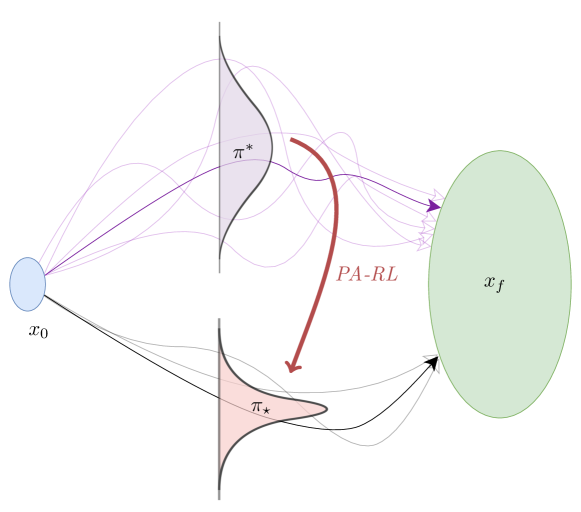
Figure 1. Qualitative representation of PARL. Reaching the green set represents policies that yield “acceptable” reward returns. Through PARL, we shift the policy synthesis towards policies that yield smaller entropy rates.

1.3. Notation

Given a set $\mathcal{A}$, $\Delta(\mathcal{A})$ denotes the probability simplex over $\mathcal{A}$, and $\mathcal{A}^{k}$ denotes the $k$-times Cartesian product $\mathcal{A}\times\mathcal{A}\times\dots\times\mathcal{A}$. If $\mathcal{A}$ is finite, $|\mathcal{A}|$ denotes its cardinality. Given two probability distributions $\mu,\nu$, we use $D_{TV}(\mu\|\nu)$ as the total variation distance between two distributions. We use $\operatorname{supp}(\mu)$ to denote the support of $\mu$. Given two vectors $\xi,\eta$, we write $\xi\succeq\eta$, if each $i$-th entry of $\xi$ is bigger than or equal to the $i$-th entry of $\eta$.

2. Background

We, first, introduce preliminary concepts employed throughout this work. For more detail on Markov chains and decision processes, the reader is referred to Puterman (2014).

2.1. Markov processes and Rewards

Definition 0 (Markov Chain).

A Markov Chain (MC) is a tuple $\mathcal{C}=(\mathcal{X},P,\mu_{0})$ where $\mathcal{X}$ is a finite set of states, $P:\mathcal{X}\times\mathcal{X}\to[0,1]$ is a transition probability measure and $\mu_{0}\in\Delta(\mathcal{X})$ is a probability distribution over initial states.

Specifically, $P(x,y)$ is the probability of transitioning from state $x$ to state $y$. $P^{t}(x,y)$ is the probability of landing in $y$ after $t$ time-steps, starting from $x$. The limit transition function is $P^{*}:=\lim_{t\to\infty}P^{t}$. We use uppercase $X_{t}$ to refer to the random variable that is the state of the random process governed by the MC at time $t$, and lower case to indicate specific states, e.g. $x\in\mathcal{X}$. Similarly, a trajectory or a path is a sequence of states $\mathbf{x}_{k}=\{x_{0},x_{1},...,x_{k}\}$, where $x_{i}\in\mathcal{X}$, and $\mathcal{P}_{k}$ denotes the set of all $(k+1)$-length paths. We also denote $X_{t:k}=\{X_{t},X_{t+1},...,X_{k}\}$. Further, we define $p:\mathcal{P}_{\infty}\to[0,1]$ as a probability measure over the Borel $\sigma$-algebra $\mathcal{B}(X_{0:\infty})$ of infinite-length paths of a MC conditioned to initial distribution $\mu_{0}$. For example, $p(X_{0}=x)\equiv\mu_{0}(x)$ is the probability of the initial state being $x$; $p(X_{0:3}=\mathbf{x}_{3})$ is the probability that the MC’s state follows the path $\mathbf{x}_{3}$.

Definition 0 (Markov Decission Process).

A Markov Decision Process (MDP) is a tuple $\mathcal{M}=(\mathcal{X},\mathcal{U},P,R,\mu_{0})$ where $\mathcal{X}$ is a finite set of states, $\mathcal{U}$ is a finite set of actions, $P:\mathcal{X}\times\mathcal{U}\times\mathcal{X}\to[0,1]$ is a probability measure of the transitions between states given an action, $R:\mathcal{X}\times\mathcal{U}\times\mathcal{X}\to\mathbb{R}$ is a bounded reward function and $\mu_{0}\in\Delta(\mathcal{X})$ is the probability distribution of initial states.

Specifically, $P(x,u,y)$ is the probability of transitioning from state $x$ to state $y$, under action $u$. A stationary Markov policy is a stochastic kernel $\pi:\mathcal{X}\to\Delta(\mathcal{U})$. With abuse of notation, we use $\pi(u\mid x)$ as the probability of taking action $u$ at state $x$, under policy $\pi$. Let $\Pi$ be the set of all stationary Markov policies, and $\Pi^{D}\subseteq\Pi$ the set of deterministic policies. The composition of an MDP $\mathcal{M}$ and a policy $\pi\in\Pi$ generates a MC with transition probabilities $P_{\pi}(x,y):=\sum_{u\in\mathcal{U}}\pi(u\mid x)P(x,u,y)$. If said MC admits a unique stationary distribution, we denote it by $\mu^{\pi}$, where $\mu^{\pi}:\mathcal{X}\to[0,1]$. We, also, use the shorthand $R_{t}^{\pi}\equiv\mathbb{E}_{u\sim\pi(x)}[R(X_{t},u,X_{t+1})]$. Finally, we consider the following assumption, which is standard in the literature of RL theory (Sutton et al., 1999; Sutton and Barto, 2018; Abounadi et al., 2001; Watkins and Dayan, 1992).

Assumption 1.

Any fixed policy $\pi$ in MDP $\mathcal{M}$ induces an aperiodic and irreducible MC.

Discounted Cumulative Reward MDPs

In discounted cumulative reward maximization problems the goal is to find a policy $\pi^{\prime}$ that maximizes the discounted sum of rewards for discount factor $\gamma\in[0,1)$: i.e. $\pi^{\prime}\in\operatorname{argmax}_{\pi\in\Pi}\mathbb{E}[\sum_{t=0}^{\infty}\gamma^{t}R_{t}^{\pi}\mid X_{0}=x]$, for all $x\in\mathcal{X}$. In the case of discounted cumulative reward maximization (Puterman, 2014), given a policy $\pi$, the value function under $\pi$, $V^{\pi}:\mathcal{X}\mapsto\mathbb{R}$, is $V^{\pi}(x):=\mathbb{E}[\sum_{t=0}^{\infty}\gamma^{t}R_{t}^{\pi}\mid X_{0}=x]$. The action-value function (or $Q$-function) under $\pi$ is given by $Q^{\pi}(x,u):=\sum_{y\in\mathcal{X}}P(x,u,y)(R(x,u,y)+\gamma V^{\pi}(y)).$

Average Reward MDPs

In average reward maximization problems, we aim at maximizing the reward rate (or gain):

(1) $$g^{\pi}(x):=\mathbb{E}\left[\lim_{T\to\infty}\frac{1}{T}\sum_{t=0}^{T}R_{t}^{\pi}\mid X_{0}=x\right],$$

i.e., we seek for $\pi^{\prime}\in\operatorname{argmax}_{\pi\in\Pi}g^{\pi}(x)$, for all $x\in\mathcal{X}$. Additionally, we define the bias as the expected difference between the stationary rate and the rewards obtained by initialising the system at a given state:

(2) $$b^{\pi}(x):=\mathbb{E}\left[\lim_{T\to\infty}\sum_{t=0}^{T}\left(R_{t}^{\pi}-g(X_{t})\right)\mid X_{0}=x\right].$$

For $\pi\in\Pi$, the average-reward value-function $V^{\pi}_{\mathrm{avg}}:\mathcal{X}\to\mathbb{R}$ is defined by (Abounadi et al., 2001) $V^{\pi}_{\mathrm{avg}}(x):=\mathbb{E}_{u\sim\pi,y\sim P(x,u,\cdot)}[R(x,u)-g^{\pi}+V_{\mathrm{avg}}^{\pi}(y)].$ The optimal value function (which exists for ergodic MDPs) satisfies $V^{*}_{\mathrm{avg}}(x)=\max_{u\in\mathcal{U}}\mathbb{E}_{y\sim P(x,u,\cdot)}\left[R(x,u)-g^{*}+V^{*}_{\mathrm{avg}}(y)\right],$ where $g^{*}$ is the optimal reward rate. Further, we the average reward action-value function $Q^{\pi}_{\mathrm{avg}}:\mathcal{X}\times\mathcal{U}\to\mathbb{R}$ is defined by $Q^{\pi}_{\mathrm{avg}}(x,u):=\mathbb{E}_{y\sim P(x,u,\cdot)}\left[R(x,u)-g^{\pi}+V^{\pi}_{\mathrm{avg}}(y)\right]$, where the optimal $Q$-function satisfies $Q^{*}_{\mathrm{avg}}(x,u)=\mathbb{E}_{y\sim P(x,u,\cdot)}\left[R(x,u)-g^{*}+V^{*}_{\mathrm{avg}}(y)\right].$

Reinforcement Learning

RL methods can be generally split in value-based and policy-based schemes. Our work considers policy-based ones. Policy-gradient algorithms usually consider policies $\pi_{\theta}$ parameterised by $\theta\in\Theta$, and write the problem of policy synthesis as a stochastic approximation scheme (Borkar, 2009). One aims to maximize over $\theta$ the objective $J(\theta):=\mathbb{E}_{\begin{subarray}{c}u\sim\pi_{\theta}\end{subarray}}\left[\rho(X_{0:T})\right]$, where $\rho$ is either the average reward or discounted cumulative reward, and $X_{0:T}$ are $T$-long trajectories (possibly $T\to\infty$). There exist several approaches to estimate $\nabla_{\theta}J(\theta)$ and update the policy parameters $\theta\leftarrow\theta+\alpha_{t}\nabla_{\theta}J(\theta)$ (Sutton and Barto, 2018; sutton_policy_nodate; Schulman et al., 2015, 2017).

2.2. Shannon Entropy and MDPs

For a discrete random variable $A$ with finite support $\mathcal{A}$, Shannon entropy (Shannon, 1948) is a measure of uncertainty induced by its distribution, and it is defined as

(3) $$h(A):=-\sum_{a\in\mathcal{A}}\Pr\left(A=a\right)\log(\Pr\left(A=a\right)).$$

Shannon entropy measures the amount of information encoded in a random variable: a uniform distribution maximizes entropy (minimal information), and a Dirac distribution minimizes it (maximal information). For an MDP under policy $\pi$, we define the conditional entropy (Cover, 1999; Biondi et al., 2014) of $X_{T+1}$ given $X_{0:T}$ as:

$$h^{\pi}(X_{T+1}\mid X_{0:T}):= -\sum_{y\in\mathcal{X},\mathbf{x}_{T}\in\mathcal{X}^{T}}p\left(X_{T+1}=y,X_{0:T}=\mathbf{x}_{T}\right)\cdot$$

$$\cdot\log(p\left(X_{T+1}=y\mid X_{0:T}=\mathbf{x}_{T}\right)),$$

and the joint entropy of the path $X_{0:T}$ is

$$h^{\pi}(X_{0:T}):= -\sum_{\mathbf{x}_{T}\in\mathcal{X}^{T}}p\left(X_{0:T}=\mathbf{x}_{T}\right)\log(p\left(X_{0:T}=\mathbf{x}_{T}\right))$$

$$= h(X_{0})+h(X_{1}\mid X_{0})+...+h(X_{T}\mid X_{0:T-1}).$$

Definition 0 (Entropy Rate (Shannon, 1948)).

Whenever the limit exists, the entropy rate of an MDP $\mathcal{M}$ under policy $\pi$ is defined by $\bar{h}^{\pi}:=\lim_{T\to\infty}\frac{1}{T}h(X_{0:T}).$

The entropy rate represents the rate of diversity in the information generated by the induced MC’s paths.

3. Problem Statement

The problem considered in this work is the following:

Problem 0.

Consider an unknown MDP $\mathcal{M}=(\mathcal{X},\mathcal{U},P,R,\mu_{0})$ and let Assumption 1 hold. Further, assume that we can sample transitions $\big{(}x,u,y,R(x,u,y)\big{)}$ applying any action $u\in\mathcal{U}$ and letting $\mathcal{M}$ evolve according to $P(x,u,\cdot)$. The objective is to find:

(4) $$\pi_{\star}\in\operatorname{argmax}\limits_{\pi\in\Pi}\mathbb{E}[\sum_{t=0}^{\infty}\gamma^{t}R_{t}^{\pi}]-k\bar{h}^{\pi},$$

where $k>0$ is a tuneable parameter.

In words, we are looking for policies that maximize a tuneable weighted linear combination of the negative entropy $-\bar{h}^{\pi}$ and a standard expected discounted cumulative reward. As such, we establish a trade-off, which is tuned via the parameter $k$, between entropy rate minimization (i.e. predictability) and optimality w.r.t. the cumulative reward.

Proposed approach

We first show how the entropy rate $\bar{h}^{\pi}$ can be treated as an average reward criterion, with the so-called local entropy $l^{\pi}$ as its corresponding local reward. Then, because $l^{\pi}$ is policy-dependent, we introduce a surrogate reward, that solely depends on states and actions and can be learned in-the-loop. We show that deterministic policies minimizing the expected average surrogate reward exist and also minimize the actual entropy rate. Moreover, we prove that, given a learned model of the MDP, we are able to (locally optimally) approximate the value function associated to the entropy rate, via learning the surrogate’s value functions. Based on these results, we propose a (model-based) RL algorithm with its maximization objective being the combination of the cumulative reward and an average reward involving the surrogate local entropy. The proofs to our results can be found in Appendix B.

4. Entropy Rates: Estimation and Learning

Towards writing the entropy rate $\bar{h}^{\pi}$ as an expected average reward, let us define the local entropy, under policy $\pi$, for state $x\in\mathcal{X}$ as

(5) $$l^{\pi}(x):=-\sum_{y\in X}P_{\pi}(x,y)\log P_{\pi}(x,y).$$

Now, making use of the Markov property, the entropy rate for an MDP reduces to

(6) $$\bar{h}^{\pi}= \lim_{T\to\infty}\frac{1}{T}\left(h(X_{0})+\sum_{t=1}^{T}h(X_{t}\mid X_{0:t-1})\right)$$

$$= \lim_{T\to\infty}\frac{1}{T}\left(h(X_{0})+\sum_{t=1}^{T}h(X_{t}\mid X_{t-1})\right)$$

$$= \lim_{T\to\infty}\frac{1}{T}\sum_{t=0}^{T}\mathbb{E}[l^{\pi}(X_{t})]=\mathbb{E}\big{[}\lim_{T\to\infty}\frac{1}{T}\sum_{t=0}^{T}l^{\pi}(X_{t})\big{]}.$$

We can treat the local entropy $l^{\pi}$ under policy $\pi$ as a policy-dependent reward (or cost) function, since $l^{\pi}$ is stationary, history independent and bounded. Thus, $\bar{h}^{\pi}$ is treated as an expected average reward, with reward function $l^{\pi}$.

4.1. A Surrogate for Local Entropy

In conventional RL settings, one is able to sample rewards (and transitions, e.g. from a simulator). However, here, part of the expected reward to be maximized in (4) is the negative entropy $-\bar{h}^{\pi}$, which, as aforementioned, can be seen as an expected average reward with a state- and policy-dependent local reward $l^{\pi}(x)$. It is not reasonable to assume that one can directly sample local entropies $l^{\pi}(x)$: one would have to estimate $l^{\pi}(x)$ through estimating transition probabilities $P_{\pi}(x,y)$ (by sampling transitions) and using (5).

However, a new challenge arises: $l^{\pi}$ depends on the policy (not on actions), and to apply average reward MDP theory we need the rewards to be state-action dependent. To address this, we consider a surrogate for $l^{\pi}$ that is policy-independent:

$$s(x,u)=-\sum_{y\in X}P(x,u,y)\log\left(P(x,u,y)\right).$$

Define $\bar{h}^{\pi}_{s}(x):=\lim_{T\to\infty}\mathbb{E}[\frac{1}{T}\sum_{t=0}^{T}s(X_{t},\pi(X_{t}))|X_{0}=x]$. The following relationships between $l^{\pi},s,\bar{h}^{\pi}$ and $\bar{h}^{\pi}_{s}$ hold:

Lemma 0.

Consider MDP $\mathcal{M}=(\mathcal{X},\mathcal{U},P,R,\mu_{0})$ and let Assumption 1 hold. The following statements hold.

1. $\mathbb{E}_{u\sim\pi(x)}[s(x,u)]\leq l^{\pi}(x)$, for all $\pi\in\Pi$.

2. $\bar{h}^{\pi}_{s}(x)=\bar{h}^{\pi}_{s}\leq\bar{h}^{\pi}$, for some $\bar{h}^{\pi}_{s}\in\mathbb{R}$, for all $\pi\in\Pi$.

3. $\mathbb{E}_{u\sim\pi(x)}[s(x,u)]=l^{\pi}(x)$ and $\bar{h}^{\pi}_{s}=\bar{h}^{\pi}$, for all $\pi\in\Pi^{D}$.

4.2. Minimum Entropy Policies through the Surrogate Local Entropy

Based on Lemma 1, we derive one of our main results:

Theorem 2.

Consider MDP $\mathcal{M}=(\mathcal{X},\mathcal{U},P,R,\mu_{0})$ and let Assumption 1. The following hold:

• There exists a deterministic policy $\hat{\pi}\in\Pi^{D}$ minimizing the surrogate entropy rate , i.e. $\hat{\pi}\in\operatorname{argmin}_{\pi}\bar{h}^{\pi}_{s}$.

• Any $\hat{\pi}\in\Pi^{D}$ minimizing the surrogate entropy rate also minimizes the true entropy rate: $\hat{\pi}\in\operatorname{argmin}_{\pi\in\Pi}\bar{h}^{\pi}_{s}$ and $\hat{\pi}\in\Pi^{D}$ $\implies\hat{\pi}\in\operatorname{argmin}_{\pi\in\Pi}\bar{h}^{\pi}$. Additionally, deterministic policies locally minimizing $\bar{h}^{\pi}_{s}$ also locally minimize $\bar{h}^{\pi}$.

• There exists a deterministic policy $\hat{\pi}\in\Pi^{D}$ such that $\hat{\pi}\in\operatorname{argmin}_{\pi}\bar{h}^{\pi}$.

Theorem 2 is an utterly relevant result for our work. First, it guarantees that minimizing policies both for $\bar{h}^{\pi}_{s}$ and $\bar{h}^{\pi}$ exist. More importantly, it tells us that, to minimize the entropy rate of an RL agent, it is sufficient to minimize the surrogate entropy rate. Since (globally) minimizing $\bar{h}^{\pi}_{s}$ implies minimizing $\bar{h}^{\pi}$ and since $s$ is policy-independent, in contrast to $l^{\pi}$, in what follows, our RL algorithm uses estimates of $s$ to minimize $\bar{h}^{\pi}_{s}$, instead of using estimates of $l^{\pi}$ to minimize $\bar{h}^{\pi}$.

5. Predictability-Awareness in Policy Gradients

In the following, we show how predictability of the agent’s behavior can be cast as an RL objective and combined with a primary discounted reward goal. Then, we derive a PG algorithm maximizing the combined objective. to address the Problem Statement.

5.1. Learning Entropy Rate Value Functions

First, we show how to cast entropy rate minimization as an RL objective, by relying on Theorem 2 and employing the surrogate entropy $s(x,u)$ as a local reward along with its corresponding value function. We prove that, given a learned model of the MDP, we are able to approximate the true entropy rate value functions. In the next section, we combine this section’s results with conventional discounted rewards and standard PG results, to address the problem mentioned in the Problem Statement and derive a PG algorithm that maximizes the combined reward objective.

We define the predictability objective to be minimized as:

$$J_{s}(\pi)\equiv\bar{h}^{\pi}_{s}=\mathbb{E}\left[\lim_{T\to\infty}\frac{1}{T}\sum_{t=0}^{T}s\big{(}X_{t},\pi(X_{t})\big{)}\right].$$

Motivated by Theorem 2, we have employed the surrogate entropy as a local reward and consider the corresponding average-reward problem. As commonly done in average reward problems, we define the (surrogate) entropy value function for a policy $\pi$, $W^{\pi}:\mathcal{X}\to\mathbb{R}$ to be equal to the bias, i.e.:

(7) $$W^{\pi}(x):= \mathbb{E}\left[\sum_{t=0}^{\infty}s\big{(}X_{t},\pi(X_{t})\big{)}-\bar{h}^{\pi}_{s}\mid X_{0}=x\right]=$$

$$= \mathbb{E}_{y\sim P_{\pi}(x,\cdot)}\left[s\big{(}x,\pi(x)\big{)}-\bar{h}^{\pi}_{s}+W^{\pi}(y)\right],$$

Additionally, we define the (surrogate) entropy action-value function $S^{\pi}:\mathcal{X}\times\mathcal{U}\to\mathbb{R}$ by $S^{\pi}(x,u):=\mathbb{E}_{y\sim P_{\pi}(x,u,\cdot)}\left[s\big{(}x,u\big{)}-\bar{h}^{\pi}_{s}+W^{\pi}(y)\right]$.

However, recall that we do not know the local reward $s$. To estimate $s$, one needs to have an estimate of the transition function $P$ of the MDP. We use

$$s_{\phi}(x,u)=-\sum_{y\in\mathcal{X}}{P}_{\phi}(x,u,y)\log\big{(}{P}_{\phi}(x,u,y)\big{)}$$

(and $\bar{h}^{\pi}_{s_{\phi}}$ correspondingly, for its associated rate) to denote the – parameterised by $\phi$ – estimate of $s$, which results from a corresponding estimate ${P}_{\phi}$ of $P$ (i.e. ${P}_{\phi}$ is the learned model). Similarly, we will use $J_{s_{\phi}}$, $W^{\pi}_{\phi}$ and $S^{\pi}_{\phi}$ to denote value functions computed with the model estimates $s_{\phi}$.

Now, it is crucial to know that by using the model estimates $s_{\phi}$ we are still able to approximate well the objective $J_{s}$ and the value functions $W^{\pi},S^{\pi}$. Let us first show that for a small error between ${P}_{\phi}$ and $P$ (i.e. small modeling error), the error between $s_{\phi}$ and $s$ and the objectives $J_{s}(\pi)\equiv\bar{h}^{\pi}_{s}$ and $J_{s_{\phi}}(\pi)\equiv\bar{h}^{\pi}_{s_{\phi}}$ is also small:

Proposition 0.

Consider MDP $\mathcal{M}=(\mathcal{X},\mathcal{U},P,R,\mu_{0})$ and let Assumption 1 hold. Consider ${P}_{\phi}:\mathcal{X}\times\mathcal{U}\times\mathcal{X}\to[0,1]$, parameterised by $\phi\in\Phi$. Assume that the total variation error between ${P}_{\phi}$ and $P$ is bounded as follows, for all $x\in\mathcal{X}$ and $u\in\mathcal{U}$:

$$\max_{x\in\mathcal{X},u\in\mathcal{U}}D_{TV}\big{(}{P}_{\phi}(x,u,\cdot)\|P(x,u,\cdot)\big{)}\leq\epsilon,$$

for some $\epsilon$, with $0\leq\epsilon\leq 1$. Then,

$$\|s_{\phi}(x,u)-s(x,u)\|_{\infty}\leq K(\epsilon),$$

and the surrogate entropy rate error for any policy $\pi$,

$$\mathbb{E}\big{[}\lim_{T\to\infty}\frac{1}{T}\sum_{t=0}^{T}s_{\phi}(X_{t},\pi(X_{t}))\mid X_{0}\sim\mu_{0}\big{]}-\bar{h}^{\pi}_{s}\leq K(\epsilon),$$

where $K(\epsilon)=\epsilon\log\big{(}|\mathcal{X}|-1\big{)}-\epsilon\log\epsilon-(1-\epsilon)\log(1-\epsilon)$.

Observe that as $\epsilon\to 0$, i.e. as the learned model approaches the real one, then the surrogate entropy rate converges to the actual one (since $K(\epsilon)\to 0$). This result indicates that we can indeed use $s_{\phi}$, obtained by a learned model $P_{\phi}$, instead of the unknown $s$, as the error between the objectives $J_{s}(\pi)\equiv\bar{h}^{\pi}_{s}$ and $J_{s_{\phi}}(\pi)\equiv\bar{h}^{\pi}_{s_{\phi}}$ is small, for small model errors.

Assume now, without loss of generality that we have parameterised entropy value function (critic) $S_{\omega}$ with parameters $\omega\in\Omega$. We show that a standard on-policy algorithm, with policy $\pi$, with value function approximation $S_{\omega}$, using the approximated model $P_{\phi}$, learns entropy value functions that are in a $\delta(\epsilon)$-neighbourhood of the true entropy value functions $S^{\pi}$, and $\delta(\epsilon)$ vanishes with $\epsilon$.

Assumption 2.

Any learning rate $\alpha_{t}\in(0,1)$ satisfies $\sum_{t=0}^{\infty}\alpha_{t}=\infty$, $\sum_{t=0}^{\infty}\alpha_{t}^{2}<\infty$.

Assumption 3.

$S_{\omega}$ is linear on $\omega$, and $\omega\in\Omega\subset\mathbb{R}^{n}$, where $\Omega$ is compact and $n>0$.

Assumption 4.

The approximated model ${P}_{\phi}$ satisfies

$$\max_{x\in\mathcal{X},u\in\mathcal{U}}D_{TV}({P}_{\phi}(x,u,\cdot)\|P(x,u,\cdot))\leq\epsilon,$$

for some (small) $\epsilon>0$.

Proposition 0.

Consider an MDP $\mathcal{M}$, a policy $\pi$, a learned model $P_{\phi}$ of the MDP and critic $S_{\omega}$. Let Assumptions 1, 3 and 4 hold. At every step $k$ of parameter iteration, let us collect trajectories of length $T$, $\mathcal{T}_{k}=\{\big{(}x^{k}_{t},u^{k}_{t},x^{k}_{t+1},s^{k}_{\phi}(x,u)\big{)}_{t=0}^{T}\}$, and construct (unbiased) estimates $\hat{S}^{\pi}_{\phi}$ such that $\mathbb{E}[\hat{S}^{\pi}_{\phi}(x,u)]=S^{\pi}_{\phi}(x,u).$ Let the critic parameters $\omega\in\Omega$ be updated in the following iterative scheme, with $\omega_{0}\in\Omega$ and $\beta_{k}$ being a learning rate satisfying Assumption 2:

$$\omega_{k+1}= \omega_{k}-\beta_{k}\hat{\Delta\omega_{k}},$$

$$\hat{\Delta\omega_{k}}= \left(\hat{S}^{\pi}_{\phi}(x_{k},u_{k})-S_{\omega}(x_{k},u_{k})\right)\frac{\partial S_{\omega}(x_{k},u_{k})}{\partial\omega}.$$

Then, the parameters $\omega$ converge to a $\delta(\epsilon)$-neighbourhood of one of the (local) minimizers of $\mathbb{E}_{\begin{subarray}{c}x\sim\mu^{\pi}\\ u\sim\pi_{\theta}(x)\end{subarray}}\left[\frac{1}{2}\left({S}^{\pi}(x,u)-S_{\omega}(x,u)\right)^{2}\right]$, where $\delta(\epsilon)$ is vanishing with $\epsilon$.

In other words, for small model errors, the value function approximator converges to a locally optimal value function approximation of the true value function $S^{\pi}$.

5.2. Predictability-Aware Policy Gradient

Now, we are ready to address the Problem Statement, combining the entropy rate objective with a discounted reward objective. In what follows, assume that we have a parameterised policy $\pi_{\theta}$ with parameters $\theta\in\Theta$. Let $J(\pi_{\theta})=\mathbb{E}[\sum_{t=0}^{\infty}\gamma^{t}R_{t}^{\pi_{\theta}}]$. We use $Q_{\xi}$ with parameters $\xi\in\Xi$ for the parameterised critic of the discounted reward objective (when using a form of actor-critic algorithm).

Theorem 3.

Consider an MDP $\mathcal{M}$, parameterised policy $\pi_{\theta}$, a learned model $P_{\phi}$ of the MDP and critic $S_{\omega}$. Let Assumptions 1, 3 and 4 hold. Let a given PG algorithm maximize (locally) the discounted reward objective $J(\pi_{\theta})=\mathbb{E}[\sum_{t=0}^{\infty}\gamma^{t}R_{t}^{\pi_{\theta}}]$. Let the value function $Q_{\xi}$ (or $V_{\xi}$) be parameterised by $\xi\in\Xi$, and the entropy value function $S_{\omega}$ (or $W_{\omega}$) have the same parameterisation class. Then, the same PG algorithm with updates

$$\theta\leftarrow\operatorname{proj}_{\Theta}\left[\theta-\alpha_{t}\left(\hat{\nabla}_{\theta}J(\pi_{\theta})+k\hat{\nabla}_{\theta}J_{s_{\phi}}(\pi_{\theta})\right)\right]$$

converges to a local minimum of the combined objective $J(\pi_{\theta})+kJ_{s_{\phi}}(\pi_{\theta}).$

Remark 1.

Regarding pure entropy rate minimization, i.e. without the discounted reward objective, as already proven by Theorem 2, a policy that is globally optimal for the surrogate entropy rate $J_{s}(\pi)$ is also optimal for the actual entropy rate $\bar{h}^{\pi}$. The same holds for locally optimal deterministic policies. However, in general, this is not the case for stochastic local minimizers.

We present now the algorithm, which combines a reward-maximizing policy gradient objective with an entropy rate objective and a model learning step. Algorithm 1 goes as follows. Following a vanilla policy gradient structure, we first sample a trajectory $\tau$ of length $T$, under a policy $\pi_{\theta}$, and store it in a buffer $\mathcal{D}$ (for training the approximate model ${P}_{\phi}$). Then, we use $\mathcal{D}$ to train ${P}_{\phi}$; update the estimated entropy rate; compute estimated objective gradients $\hat{\nabla}_{\theta}J(\pi_{\theta}),\,\hat{\nabla}_{\theta}J_{s_{\phi}}(\pi_{\theta})$ from trajectory $\tau$; and finally update the policy parameters and critics $S_{\omega},Q_{\xi}$.

Algorithm 1 Predictability Aware Policy Gradient

0:  ${P}_{\phi},\pi_{\theta}$, critics $W_{\omega}$, $V_{\xi}$

0:  $\alpha_{t}$, $k>0$

  for $E$ epochs do

     $\mathcal{D}\leftarrow$ Trajectory $\tau$ of length $T$.

     Train ${P}_{\phi}$ from $\mathcal{D}$.

     $\bar{h}^{\pi}_{s_{\phi}}\leftarrow\frac{1}{T}\sum_{x,u\in\tau}s_{\phi}(x,u)$.

     Compute estimations $\hat{\nabla}_{\theta}J(\pi_{\theta}),\,\hat{\nabla}_{\theta}J_{s_{\phi}}(\pi_{\theta})$ from $\tau$.

     $\theta\leftarrow\operatorname{proj}_{\Theta}\left[\theta-\alpha_{t}\left(\hat{\nabla}_{\theta}J(\pi_{\theta})+k\hat{\nabla}_{\theta}J_{s_{\phi}}(\pi_{\theta})\right)\right]$

     Update $S_{\omega}$ (and $Q_{\xi}$ if used)

  end for

5.3. Implementation: Predictability-Aware PPO

Policy Learning

We propose implementing our predictability-aware scheme into an average-reward PPO algorithm (Ma et al., 2021). In particular, for every collected trajectory $\tau$, we update the estimate $\bar{h}^{\pi}_{s_{\phi}}$ and (surrogate) entropy value function $W_{\omega}$ parameterised by $\omega\in\Omega$ from the collected samples, and we compute entropy advantages for all $(x,u,y,s_{\phi}(x,u))$ in the collected trajectories as:

(8) $$\hat{A}_{s}^{\pi}=s_{\phi}(x,u)-\bar{h}^{\pi}_{s_{\phi}}+W_{\omega}(y)-W_{\omega}(x).$$

Then we apply the gradient steps as in PPO (Schulman et al., 2015, 2017) by clipping the policy updates.

Model Learning

To learn the approximated model ${P}_{\phi}$, we assume the transitions to follow Gaussian distributions, similarly to Janner et al. (2019). Following the definition of entropy of a continuous Gaussian distribution, $s_{\phi}(x,u)=\log(\sigma^{2}_{xu})+K,$ where $K=\frac{1}{2}\big{(}\log(2\pi)+1)$. Therefore, we can estimate the entropy directly by the variance output of our model. Furthermore, since we only need to estimate the variance per transition $(x,u)\to y$, it is sufficient to construct a model $f_{\phi}:\mathcal{X}\times\mathcal{U}\to\mathcal{X}$ that approximates the mean $f_{\phi}(x,u)\approx\int yP(x,u,y)dy$, and we do this through minimizing a mean-squared error loss of transition samples in our model. Then, we estimate the entropy of an observed transition as $s_{\phi}(x,u)=\log(\mathbb{E}_{y\sim P(x,u,\cdot)}[(f_{\phi}(x,u)-y)^{2}])$.

Remark 2.

This is an important feature that greatly simplifies the practical implementation of our approach. Learning models of dynamical systems is notoriously difficult (Moerland et al., 2022; Janner et al., 2019) in general RL environments, as transitions might follow very complex distributions. In our case, to estimate the entropy (and thus the predictability) we only need to learn a model that predicts the mean of each transition, and we reconstruct the entropy from the sampled trajectories.

6. Experiments

We implemented PARL on a set of robotics and autonomous driving tasks, evaluated the obtained rewards and entropy rates, and compared against different baselines. To the best of our knowledge, there are no other RL algorithms that attempt to increase predictability by optimising entropy rates, and thus it is not possible to compare predictability scores against other recent algorithms.

6.1. Predictable Driving

We test PARL in the Highway Environment (Leurent, 2018), where an agent learns to drive at a desired speed while navigating a crowded road with other autonomous agents. The agent gets rewarded for tracking the desired speed and penalised for collisions. We consider a highway and a roundabout scenario (see Figure 2). We compare against PPO (Schulman et al., 2017) and DQN (Mnih et al., 2015)) agents, and take the hyperparameters directly from Leurent (2018). The results are presented in Table 1.

Figure 2. Self-Driving Environments.

Table 1. Results for autonomous driving environments.

Highway	Rewards	Ep. Length	Avg. Speed	Entropy Rate
DQN	17.51 $\pm$ 7.73	20.92 $\pm$ 9.08	6.51 $\pm$ 0.34	-0.37 $\pm$ 0.16
PPO	18.88 $\pm$ 6.74	24.41 $\pm$ 8.49	5.62 $\pm$ 0.10	-0.88 $\pm$ 0.05
PARL ($k=0.1$)	21.05 $\pm$ 4.03	28.56 $\pm$ 5.27	5.11 $\pm$ 0.05	-1.43 $\pm$ 0.09
PARL ($k=0.5$)	21.03 $\pm$ 2.05	29.60 $\pm$ 2.64	5.06 $\pm$ 0.01	-1.51 $\pm$ 0.09
PARL ($k=1$)	20.89 $\pm$ 2.05	29.61 $\pm$ 2.58	5.05 $\pm$ 0.00	-1.51 $\pm$ 0.06

Roundabout	Rewards	Ep. Length	Avg. Speed	Entropy Rate
DQN	22.53 $\pm$ 11.93	26.92 $\pm$ 14.41	3.09 $\pm$ 0.47	-0.55 $\pm$ 0.88
PPO	29.26 $\pm$ 10.68	32.92 $\pm$ 11.67	2.80 $\pm$ 0.12	-0.23 $\pm$ 0.27
PARL ($k=0.1$)	28.86 $\pm$ 10.96	32.98 $\pm$ 12.23	2.65 $\pm$ 0.50	-0.28 $\pm$ 0.77
PARL ($k=0.5$)	17.99 $\pm$ 13.34	23.45 $\pm$ 17.60	3.75 $\pm$ 0.05	-2.13 $\pm$ 0.12
PARL ($k=1$)	16.83 $\pm$ 13.28	22.05 $\pm$ 17.67	3.79 $\pm$ 0.04	-2.21 $\pm$ 0.14

Reward vs Entropy

The agents minimise the entropy rate in both environments, resulting in more predictable driving patterns. In the highway environment, agents slow down their speed and stop overtaking. This, also, results in longer episode lengths (and larger episodic rewards), but lower rewards per time-step (caused by the fact that reward is given for driving faster). In the roundabout scenario, a different behavior emerges. Agents keep a constant high speed to traverse the roundabout as fast as possible, as the roundabout is the main source of uncertainty and complexity.

6.2. MuJoCo Environments

We test our algorithm on three MuJoCo tasks which are notoriously complex. Please note that these are deterministic. Under perfect models, all policies would have a zero entropy rate, and PARL would have no effect in the behavior of the agents. However, given that the models are learned through function approximators, PARL results in agents shifting their behaviors towards less complex trajectories, which are easier for models to learn and predict.

Table 2. Results for MuJoCo environments.

Walker2d	Rewards	Ep. Length	Entropy Rate
PPO	2466.27 $\pm$ 1329.71	638.29 $\pm$ 296.82	1.19 $\pm$ 0.40
PARL ($k=0.05$)	2430.12 $\pm$ 1199.45	626.77 $\pm$ 263.34	0.36 $\pm$ 0.74
PARL ($k=0.1$)	2047.30 $\pm$ 1106.09	551.40 $\pm$ 252.01	0.06 $\pm$ 0.61
PARL ($k=0.25$)	1315.47 $\pm$ 910.03	550.18 $\pm$ 296.42	-1.26 $\pm$ 1.79
PARL ($k=0.5$)	1072.88 $\pm$ 980.41	648.38 $\pm$ 358.74	-1.90 $\pm$ 1.16

Ant	Rewards	Ep. Length	Entropy Rate
PPO	2459.29 $\pm$ 1411.75	734.79 $\pm$ 342.21	0.80 $\pm$ 0.27
PARL ($k=0.05$)	2510.29 $\pm$ 1504.11	774.54 $\pm$ 343.79	0.66 $\pm$ 0.24
PARL ($k=0.1$)	2107.21 $\pm$ 1195.23	786.88 $\pm$ 330.96	-0.04 $\pm$ 1.64
PARL ($k=0.25$)	1497.67 $\pm$ 854.79	950.96 $\pm$ 186.39	-3.54 $\pm$ 3.04
PARL ($k=0.5$)	1204.47 $\pm$ 1076.30	987.53 $\pm$ 87.62	-5.00 $\pm$ 1.98

HalfCheetah	Rewards	Ep. Length	Entropy Rate
PPO	4150.53 $\pm$ 1645.16	1000.0 $\pm$ 0.0	1.01 $\pm$ 0.34
PARL ($k=0.05$)	3575.56 $\pm$ 1743.91	1000.0 $\pm$ 0.0	0.46 $\pm$ 0.45
PARL ($k=0.1$)	4482.48 $\pm$ 1679.52	1000.0 $\pm$ 0.0	0.31 $\pm$ 0.25
PARL ($k=0.25$)	4427.07 $\pm$ 1930.60	1000.0 $\pm$ 0.0	-0.27 $\pm$ 0.74
PARL ($k=0.5$)	3962.70 $\pm$ 1822.80	1000.0 $\pm$ 0.0	-0.54 $\pm$ 0.99

Reward vs Entropy

Note that the entropy rate reported here is the one associated to the learned model, when coupled with the learned policy (recall that the true model here is deterministic, and if the policy is deterministic, as well, entropy rate is trivially 0). Observe that, as expected, the reward-entropy trade-off becomes explicit as we increase the value of $k$. However, interestingly, for some environments the rewards actually increase when adding predictability objectives. In particular, for HalfCheetah, the highest rewards (a 10% increase) are attained for $k=0.1$. This can be explained by the fact that the MuJoCo tasks are very nonlinear, and policies are often pushed to over-fit and develop unnecessarily complex behaviors, whereas PARL rewards less complex behaviors, which are, in turn, easier to predict.

6.3. Trajectory Distribution Projections

To showcase the effect of entropy-rate minimization and PARL on trajectory distributions, we present Figures 3 and 4. We evaluated trained agents over 1000 steps, and since the trajectories are high-dimensional, computed a PCA decomposition and plotted the first two components as a projection of the trajectory.

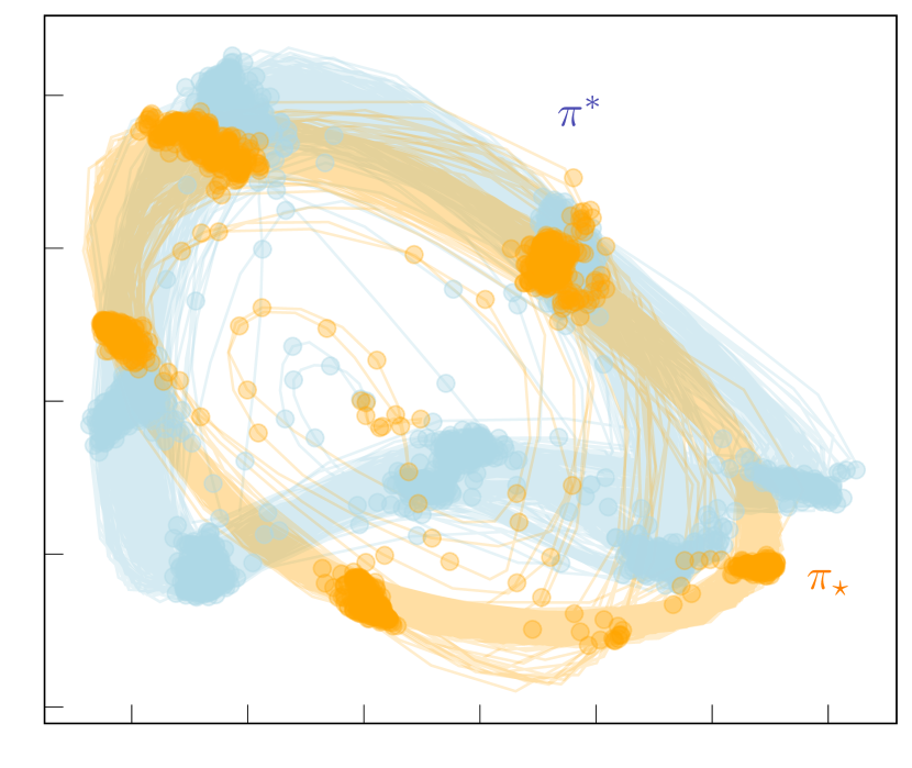
(a) HalfCheetah

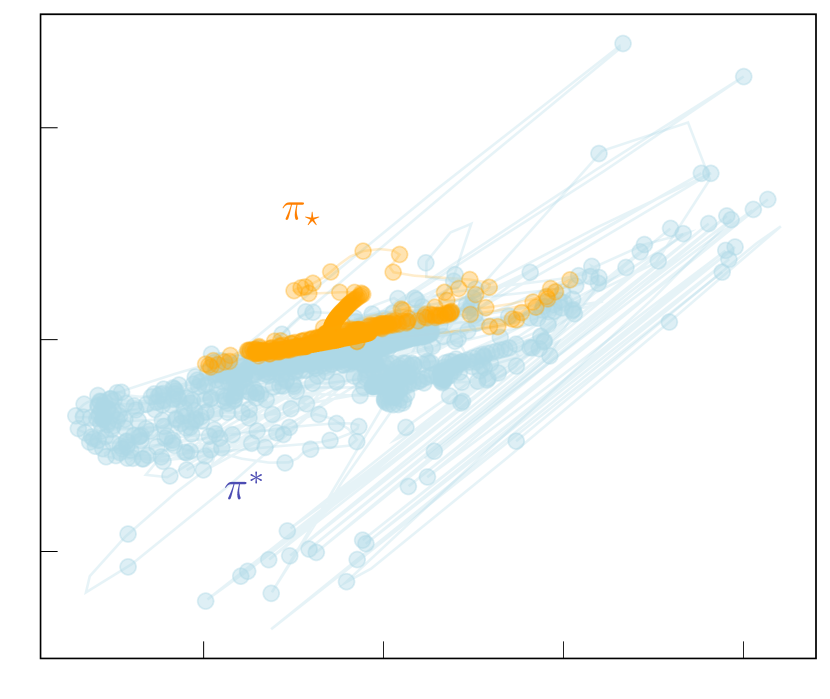
(b) Walker2d

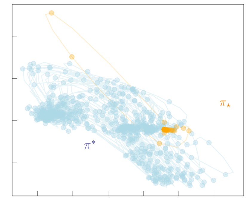
(c) Ant-v4

Figure 3. 2D trajectory projections for MuJoCo tasks. Blue is a PPO policy, orange is a PARL policy with $k=0.25$.

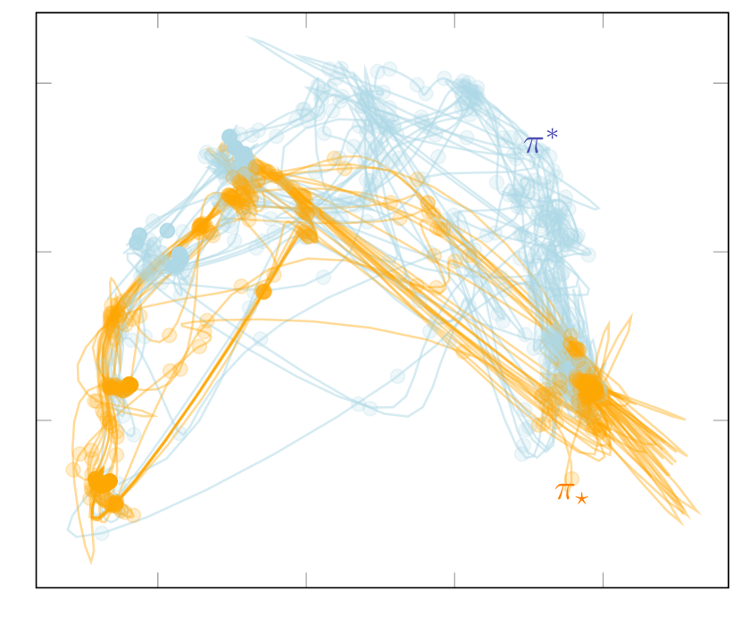
(a) Roundabout Env.

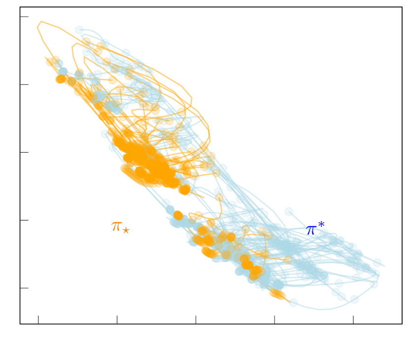
(b) Highway Env.

Figure 4. 2D trajectory projections for autonomous driving. Blue is a PPO policy, orange is a PARL policy with $k=0.5$.

In both cases, we observe that PARL policies induce more regular, clustered trajectories, which suggests much lower trajectory aleatoric uncertainty. Generally, PARL trajectories have considerably smaller variance, and visit a smaller portion of the state-space. For example, in the case of HalfCheetah, it can be seen how PARL trajectories are smoother and less complex when compared to PPO. In the Walker and Ant environments this difference is very pronounced, as PARL trajectories are concentrated in a very small region of the state-space.

7. Discussion

Summary of Results

We proposed a novel method, namely PARL, that induces more predictable behavior in RL agents. This is achieved by maximizing a tuneable linear combination of a standard expected reward and the negative entropy rate, thus trading-off optimality with predictability. We implemented the method using a modified model-based version of PPO. In the experimental results, we see how PARL greatly reduces the entropy rates of the RL agents while achieving near-optimal rewards, depending on the trade-off parameter. In the autonomous driving setting, agents learn to be more predictable while driving around stochastic agents. In the MuJoCo experiments, PARL obtains policies that yield more clustered, less complex trajectory distributions, allowing models to predict better the dynamics.

Shortcomings

Our scheme results in a setting where agents maximize a trade-off between two different objectives. This, combined with learning a dynamic model (which is notoriously difficult), introduces implementation challenges related to learning multiple coupled models simultaneously. We make an attempt at discussing a systematic way of addressing these in the Appendix. Additionally, for many applications, avoiding high-entropy policies may restrict the ability of RL agents to learn optimal behaviors (see, e.g., results in Eysenbach et al. (2021)). Although, in human-robot interaction and human-aligned AI, predictability is intuitively beneficial (for safety purposes, as mentioned before), we do not claim that introducing entropy-rate minimization is desirable for all RL applications.

Entropy and Exploration

One might wonder if minimizing entropy rates of RL agents may hinder exploration. From a theoretical perspective, this is not a problem, due to ergodicity. From a practical perspective, this undesired effect is highly mitigated by the fact that for the first (many) steps, the agent is still learning an adequate model of the dynamics, and therefore the entropy signal is very noisy which favors exploration.

Appendix A Auxiliary Results

We include in this Appendix some existing results used throughout our work. The following Theorem is a combination of results presented by (Puterman, 2014) regarding the existence of optimal average reward policies.

Theorem 1 (Average Reward Policies (Puterman, 2014)).

Given an MDP $\mathcal{M}$ and Assumption 1, the following hold: $g^{\pi}(x)$ and $b^{\pi}(x)$ exist, $g^{\pi}(x)=g^{\pi}$ for all $x$ (i.e. $g^{\pi}(x)$ is constant), and there exists a deterministic, stationary policy $\hat{\pi}\in\operatorname{argmax}_{\pi\in\Pi}g^{\pi}$ that maximizes the expected average reward. Additionally, the same holds if $\mathcal{U}$ is compact and $R$ and $P$ are continuous functions of $\mathcal{U}$.

Theorem 2 (Stochastic Recursive Inclusions (Borkar, 2009)).

Let $x_{n}\in\mathbb{R}^{d}$ be a vector following a sequence:

(9) $$x_{n+1}=x_{n}+a_{n}(h(x_{n})+M_{n+1}+\eta_{n}),$$

where $\sup_{n}\|x_{n}\|<\infty$ a.s., $a_{n}$ is a learning rate satisfying Assumption 2, $h:\mathbb{R}^{d}\to\mathbb{R}^{d}$ is a Lipschitz map, $M_{n}$ is a Martingale difference sequence with respect to the $\sigma-$algebra $\mathcal{F}_{n}:=\sigma(x_{0},M_{1},M_{2},...,M_{n})$ (and square integrable), and $\eta_{n}$ is an error term bounded by $\epsilon_{0}$. Define $H:=\{x\in\mathbb{R}^{d}:h(x)=0\}$. Then, for any $\delta>0$, there exists an $\epsilon>0$ such that $\forall\epsilon_{0}\in(0,\epsilon)$ the sequence $\{x_{n}\}$ converges almost surely to a $\delta$-neighbourhood of $H$.

Theorem 3 (Policy Gradient with Function Approximation (Sutton et al., 1999)).

Let $\pi_{\theta}$ be a parameterised policy and $f_{w}:\mathcal{X}\times\mathcal{U}\to\mathbb{R}$ be a parameterised (approximation of) action value function in an MDP $\mathcal{M}$. Let the parameterisation be compatible, i.e. satisfy:

$$\frac{\partial f_{w}(x,u)}{\partial w}=\frac{\partial\pi_{\theta}(x,u)}{\partial\theta}\frac{1}{\pi_{\theta}(x,u)}.$$

Let the parameters $w$ and $\theta$ be updated at each step such that:

$$w_{k}:\sum_{x}\mu^{\pi_{\theta}}(x)\sum_{u}\pi_{\theta}(x,u)\big{(}Q^{\pi_{\theta}}(x,u)-$$

$$-f_{w_{k}}(x,u)\big{)}\frac{\partial f_{w}(x,u)}{\partial{w_{k}}}=0,$$

$$\theta_{k+1}=\theta_{k}+\alpha_{t}\sum_{x}\mu^{\pi_{\theta}}(x)\sum_{u}\frac{\partial\pi_{\theta}(x,u)}{\partial\theta}f_{w_{k}}(x,u).$$

Then, $\lim_{k\to\infty}\frac{\partial\rho(\theta_{k})}{\partial\theta}=0$, where $\rho(\theta)$ is either the discounted or average reward in the MDP.

Appendix B Technical Proofs

Proof of Lemma 1.

For statement 1, observe $l^{\pi}(x)$ can be expressed as

$$l^{\pi}(x)= -\mathbb{E}\left[P(x,u,y)|u\sim\pi(x)\right]$$

$$\cdot\log\big{(}\mathbb{E}\left[P(x,u,y)|u\sim\pi(x)\right]\big{)},$$

and recall

$$\mathbb{E}_{u\sim\pi(x)}[s(x,u)]=$$

$$-\mathbb{E}_{u\sim\pi(x)}\big{[}\sum_{y\in X}P(x,u,y)\log\left(P(x,u,y)\right)\big{]}.$$

Then, from Jensen’s inequality, $\mathbb{E}_{u\sim\pi(x)}[s(x,u)]\leq l^{\pi}$.

In Statement 2, the fact that $\bar{h}^{\pi}_{s}(x)$ is constant follows from Theorem 1 by considering $R(x,u)\equiv s(x,u)$. Now, note that we can write $\bar{h}^{\pi}_{s}=\sum_{x\in\mathcal{X}}\mathbb{E}_{u\sim\pi(x)}[s(x,u)]\mu^{\pi}(x)$ and $\bar{h}^{\pi}=\sum_{x\in\mathcal{X}}l^{\pi}(x)\mu^{\pi}(x)$ (see (Puterman, 2014)). Thus:

$$\bar{h}^{\pi}_{s}=\sum_{x\in\mathcal{X}}\mathbb{E}_{u\sim\pi(x)}[s(x,u)]\mu^{\pi}(x)\leq$$

$$\sum_{x\in\mathcal{X}}l^{\pi}(x)\mu^{\pi}(x)=\bar{h}^{\pi},$$

where we employed Statement 1.

For Statement 3, take $\pi\in\Pi^{D}$. Then, $\pi(u^{\prime}\mid x)=1$ and $\pi(u\mid x)=0$ for an action $u^{\prime}\in\mathcal{U}$ and all $u\neq u^{\prime}$. Then

$$\mathbb{E}_{u\sim\pi(x)}[s(x,u)]= \sum_{y\in X}P(x,u^{\prime},y)\log\left(P(x,u^{\prime},y)\right)=$$

$$l^{\pi}(x).$$

The fact that $\bar{h}^{\pi}_{s}=\bar{h}^{\pi}$ follows, then, trivially. ∎

Proof of Theorem 2.

The first statement follows directly from Theorem 1, which guarantees that there is at least one deterministic policy $\hat{\pi}$ that minimizes the surrogate entropy rate $\bar{h}^{\pi}_{s}$. Then, since $\hat{\pi}\in\Pi^{D}$, from Lemma 1 statements 2 and 3, we have that the following holds for all $\pi\in\Pi$:

$$\bar{h}^{\hat{\pi}}=\bar{h}^{\hat{\pi}}\leq\bar{h}^{\pi}_{s}\leq\bar{h}^{\pi}$$

Thus, $\hat{\pi}$ minimizes $\bar{h}^{\pi}$ and it follows that $\hat{\pi}\in\operatorname{argmin}_{\pi\in\Pi}\bar{h}^{\pi}_{s}$ and $\hat{\pi}\in\Pi^{D}$ $\implies\hat{\pi}\in\operatorname{argmin}_{\pi\in\Pi}\bar{h}^{\pi}$. The same argument also applies locally, thereby yileding that deterministic local minimizers of $\bar{h}^{\pi}_{s}$ are also local minimizers of $\bar{h}^{\pi}$. Finally, the third statement follows as a combination of the other two. ∎

Proof of Proposition 1.

Observe that $s(x,u)$ and $s_{\phi}(x,u)$ are the entropies of probability distributions $P(x,u,\cdot)$ and $P_{\phi}(x,u,\cdot)$, respectively. Thus, from the Fannes–Audenaert inequality (Fannes, 1973), for the special case of diagonal density matrices (representing conventional probability distributions), we obtain:

$$\|s_{\phi}(x,u)-s(x,u)\|_{\infty} \leq$$

$$\epsilon\log\Big{(}|\mathcal{X}|-1\Big{)}-\epsilon\log\epsilon-(1-\epsilon)\log(1-\epsilon) =$$

$$=K(\epsilon),$$

Finally:

$$\mathbb{E}\big{[}\lim_{T\to\infty}\frac{1}{T}\sum_{t=0}^{T}s_{\phi}(X_{t},\pi(X_{t}))\mid X_{0}\sim\mu_{0}\big{]}-\bar{h}^{\pi}_{s}=$$

$$\mathbb{E}\big{[}\lim_{T\to\infty}\frac{1}{T}\sum_{t=0}^{T}s_{\phi}(X_{t},\pi(X_{t}))-s(X_{t},\pi(X_{t}))\big{]}\leq$$

$$\mathbb{E}\Big{[}\lim_{T\to\infty}\frac{1}{T}\sum_{t=0}^{T}\big{|}s_{\phi}(X_{t},\pi(X_{t}))-s(X_{t},\pi(X_{t}))\big{|}\Big{]}\leq$$

$$\mathbb{E}\big{[}\lim_{T\to\infty}\frac{1}{T}\sum_{t=0}^{T}K(\epsilon)\big{]}=$$

$$K(\epsilon).\quad$$

∎

Proof of Proposition 2.

Since $S_{\omega}$ is linear on $\omega\in\Omega$ and $\Omega$ is compact, there exists at least one minimizer $\omega^{*}$. Now, from (2) and Theorem 8.2.6 (Puterman, 2014), $S^{\pi}$ and $S^{\pi}_{\phi}$ can be written in vector form (over the states $\mathcal{X}$) as:

$$S^{\pi}=(I-P_{\pi}+P_{\pi}^{*})^{-1}(I-P_{\pi}^{*})s^{\pi},$$

$$S^{\pi}_{\phi}=(I-P_{\pi}+P_{\pi}^{*})^{-1}(I-P_{\pi}^{*})s_{\phi}^{\pi},$$

where $s^{\pi}$ is the vector representation of $s(\cdot,\pi(\cdot))$ (and analogously for $s^{\pi}_{\phi}$). Therefore, from Corollary 1, $\|S^{\pi}(x)-S^{\pi}_{\phi}(x)\|_{\infty}\leq K(\epsilon)$. Then, we can write without loss of generality

$${S}^{\pi}(x,u)=S^{\pi}_{\phi}(x,u)+\eta(\epsilon),$$

with $\eta(\epsilon)$ being $O(\epsilon)$. Finally, we can write the parameter iteration as

$$\omega_{t+1}=\omega_{t}+\beta_{t}\big{[}-\nabla_{\omega}L_{\omega}^{\pi}+M_{t+1}+\eta(\epsilon)\big{]},$$

with $L_{\omega}^{\pi}:=\mathbb{E}_{\begin{subarray}{c}x\sim\mu^{\pi}\\ u\sim\pi_{\theta}(x)\end{subarray}}\left[\frac{1}{2}\left({S}^{\pi}(x,u)-S_{\omega}(x,u)\right)^{2}\right]$ and the term $M_{t+1}:=\left(\hat{S}^{\pi}(x,u)-S^{\pi}(x,u)\right)\frac{\partial S_{\omega}(x,u)}{\partial\omega}$ is a Martingale with bounded variance (since $s$ is bounded).

Therefore, by Theorem 6 in (Borkar, 2009), the iterates converge to some point $\omega_{t}\to\Omega^{*}_{\delta}(\pi_{\theta})$ almost surely as $t\to\infty$, with $\Omega^{*}_{\delta}(\pi_{\theta})$ being the $O(\delta)$ neighbourhood of the stationary points satisfying $\nabla_{\omega}L_{\omega}^{\pi}=0$. ∎

Proof of Theorem 3.

By standard PG arguments (Sutton et al., 1999), if a PG algorithm converges to a local minimum of the objective $J(\pi_{\theta})$ then the updates $\hat{\nabla}_{\theta}J(\pi_{\theta})$ are in the direction of the gradient (up to stochastic approximation noise). By the same arguments, given Proposition 2, the same algorithm converges to a local minimum of the entropy value function $W_{\omega}$ through updates $\hat{\nabla}_{\theta}J_{s}(\pi_{\theta})$, and these are in the direction of the true gradient (again, up to stochastic approximation noise). Then, the linear combination of gradient updates $\hat{\nabla}_{\theta}J(\pi_{\theta})+k\hat{\nabla}_{\theta}J_{s}(\pi_{\theta})$ are in the direction of the gradient of the combined objective $J(\pi_{\theta})+kJ_{s}(\pi_{\theta})$. Finally, since both objectives are locally convex (necessary condition following from existence of gradient schemes that locally minimize them), their linear combination is also locally convex. This concludes the proof. ∎

Appendix C Experimental Results and Methodology

C.1. Extended results

We present here the extended experimental results, training curves and additional details corresponding to the experimental framework.

C.2. Interactive Robot Tasks

We created two tasks inspired by real human-robot use-cases, where it is beneficial for agents to avoid high entropy state-space regions. These are based on Minigrid environments (Chevalier-Boisvert et al., 2023), see Figure 5. The agents can execute actions $\mathcal{U}=\{\text{forward},\text{turn-left},\text{turn-right},\text{toggle}\}$, and the observation space is $\mathcal{X}=\mathbb{R}^{n}$ such that the observation includes the robot’s position and orientation, the position of obstacles and the state of environment features (e.g. the switch). In both tasks, the agent gets a reward of $1$ for reaching the goal, or a negative reward of $-1$ for colliding or falling in the lava. Both grid environments were wrapped in a normalizing vectorized wrapper, to normalize observations, but the model data was kept un-normalized.

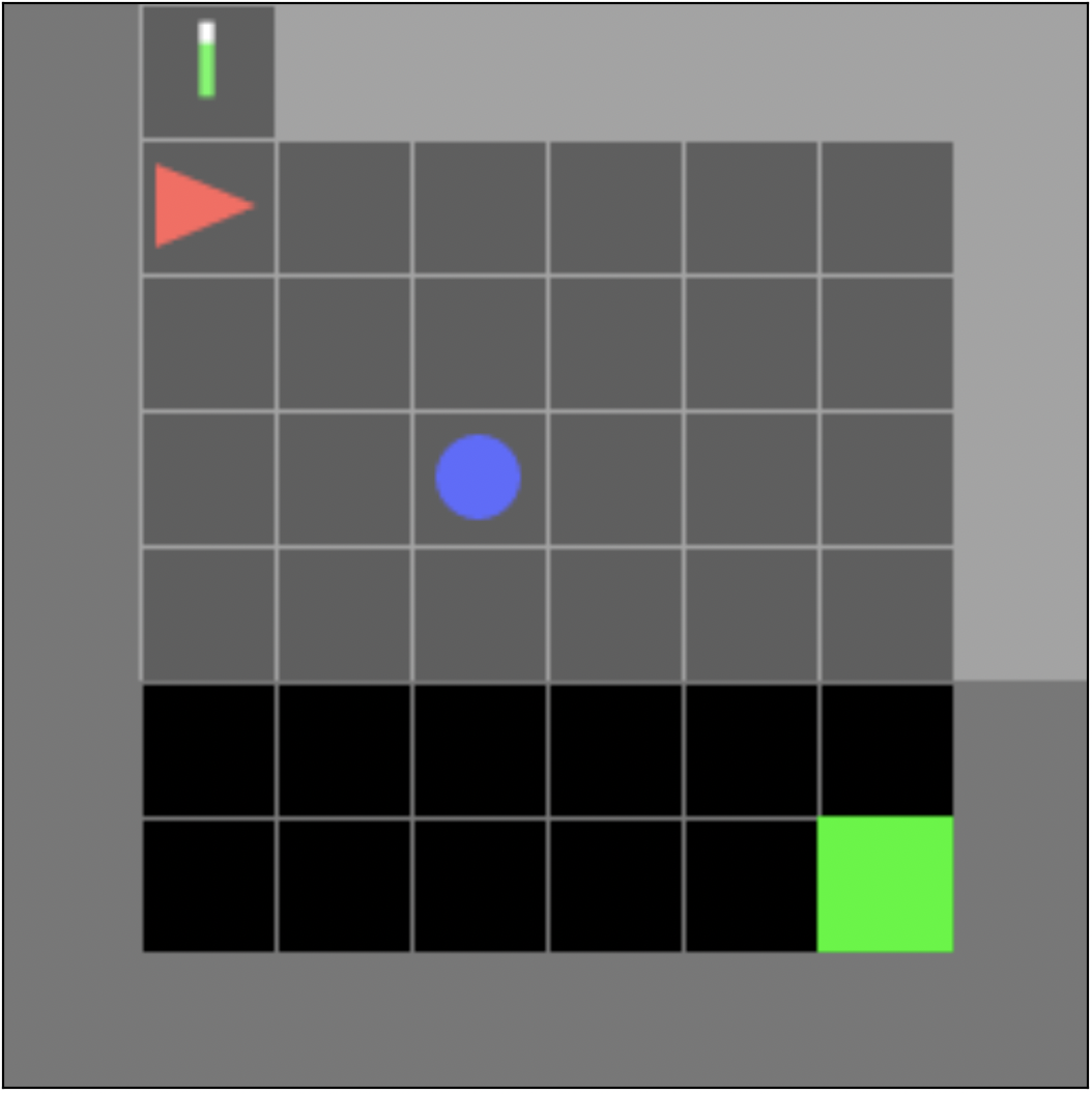
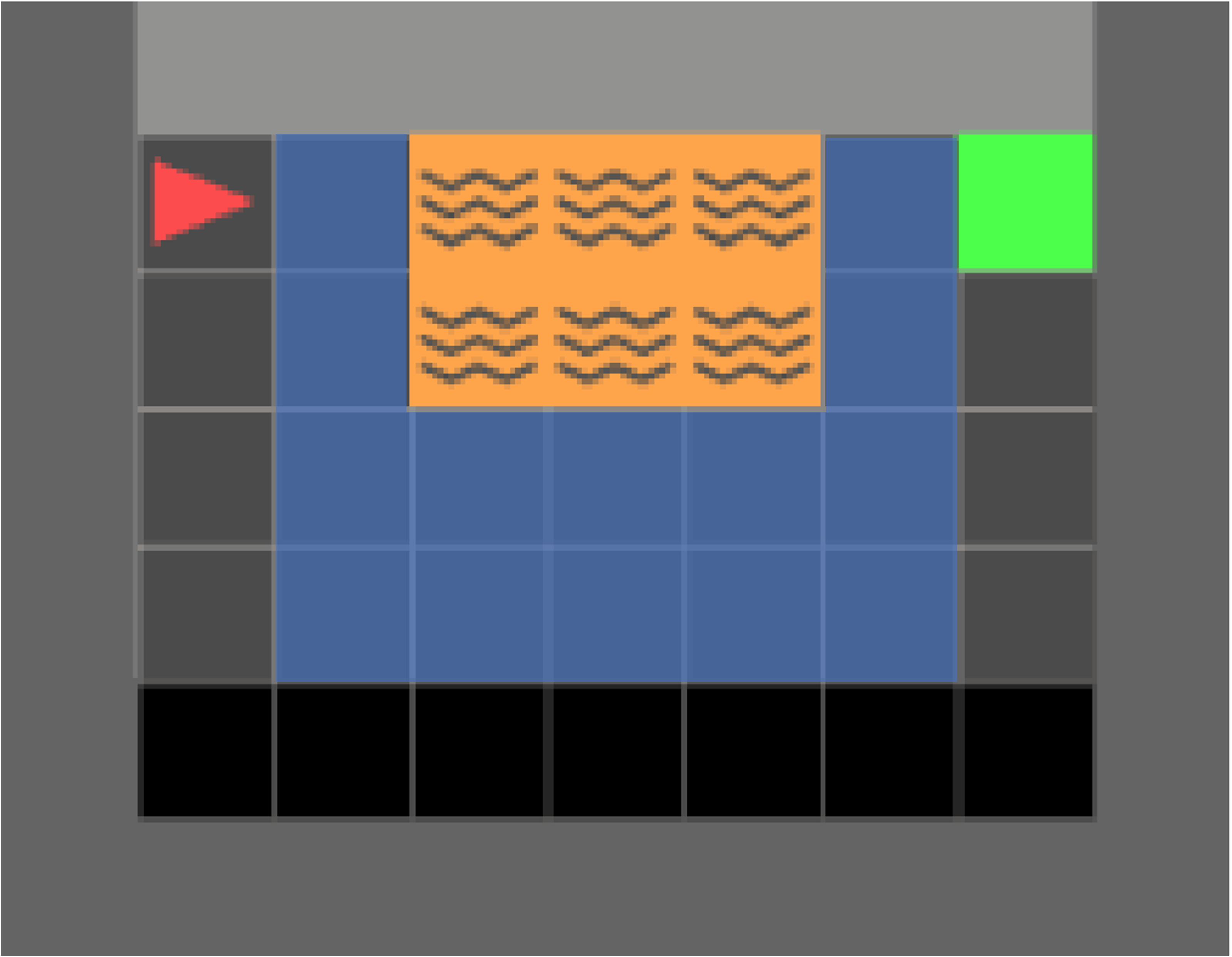
Figure 5. Interactive Tasks. Left is a moving obstacle navigation task where the agent has the option to de-activate the obstacles. Right is a navigation problem where the ground is slippery, resulting in random motion.

Task 1: Turning Off Obstacles

This task is designed as a dynamic obstacle navigation task, where the motion of the obstacles can be stopped (the obstacles can be switched off) by the agent toggling a switch at a small cost of rewards. The environment is depicted in Figure 5 (left). The switch is to the left of the agent, shown as a green bar (orange if off). The agent gets a reward of $r=0.95$ if it turns the obstacle off. The intuition behind this task is that agents do not learn to turn off the obstacles, and attempt to navigate the environment. This, however, induces less predictable dynamics since the obstacle keeps adding noise to the observation, and the agent is forced to take high variance trajectories to avoid it. Our Predictability-Aware algorithm converges to policies that consistently disable the stochasticity of the obstacles, navigating the environment freely afterwards, while staying near-optimal.

Task 2: Slippery Navigation

The second task is inspired by a cliff navigation environment, where a large portion of the ground is slippery, but a path around it is not. In this problem, the slippery part has uncertain transitions (i.e. a given action does not yield always the same result, because the robot might slip), but the non-slippery path induces deterministic behavior (the robot follows the direction dictated by the action). The agent needs to navigate to the green square avoiding the lava. If it enters the slippery region, it has a probability of $p=0.35$ of spinning and changing direction randomly. The intuition behind this environment is that PPO agents do not learn to avoid the slippery regions, resulting in higher entropy rates and less predictable behaviors. On the contrary, PARL agents consistently avoid the slippery regions. This can be seen in Figure 6.

Trajectory Representations

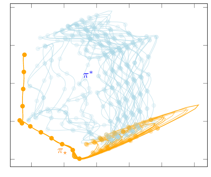
(a) Dynamic Obstacle Env.

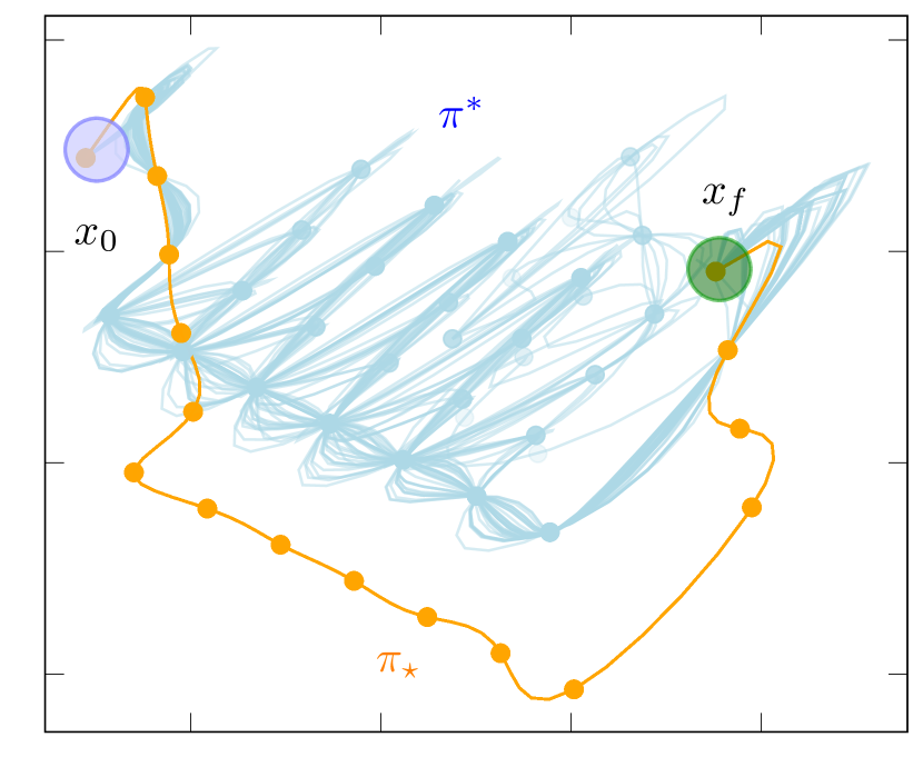
(b) Slippery Nav. Env.

Figure 6. 2D trajectory projections. Blue is a PPO policy, orange is a PARL policy.

As expected, the observed trajectories for the case of PARL agents present a much less complex (lower entropy) distribution. In particular, for the slippery navigation task where agents have the choice of taking fully deterministic paths, it is even more obvious that the PARL agent chooses to execute the same trajectory over and over, where PPO agents result in a more complex distribution due to the traversing of the stochastic regions.

C.3. Learning Results

We include the learning curves for the trained agents on all the environments included in the paper.

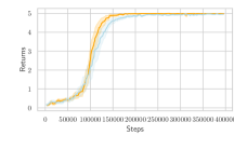
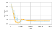
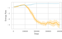
Figure 7. Training results for Slippery Navigation task.

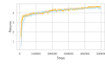
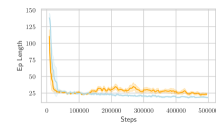
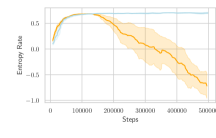
Figure 8. Training results for Obstacle Navigation task.

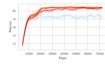
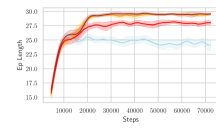
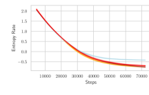
Figure 9. Training results for Highway environment.

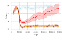
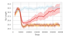
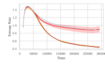
Figure 10. Training results for Roundabout environment.

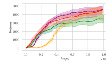
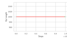
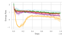
Figure 11. Training results for HalfCheetah-v4 environment.

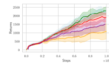
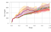
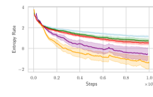
Figure 12. Training results for Walker2d-v4 environment.

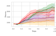
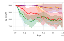
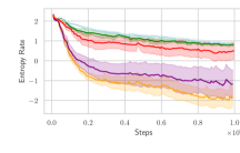
Figure 13. Training results for Ant-v4 environment.

C.4. Model Learning

Our proposed predictable RL scheme consists of a model-based architecture where the agent learns simultaneously a model $P_{\phi}$ for the transition function and a policy $\pi_{\theta}$ and value functions $V_{\xi}$, $W_{\omega}$ for the discounted rewards and entropy rates. Simultaneously to a policy and a value function, we learn a model $P_{\phi}$ to approximate the transitions (means) in the environment. For this, we train a neural network with inputs $(x,u)\in\mathcal{X}\times\mathcal{U}$ and outputs the mean next state $\bar{y}_{xu}$. The model is trained using the MSE loss for stored data $\mathcal{D}=\{(x,u,y)\}$:

$$\mathcal{L}_{y}=\frac{1}{2|\mathcal{D}|}\sum_{\mathcal{D}}\big{(}\bar{y}_{xu}-y\big{)}^{2}.$$

We do this by considering $\mathcal{D}$ to be a replay buffer (to reduce bias towards current policy parameters), and at each iteration we perform $K$ mini-batch updates of the model sampling uniformly from the buffer. Additionally, we pre-train the model a set number of steps before beginning to update the agents, by running a fixed number of environment steps with a randomly initialised policy, and training the model on this preliminary data. All models are implemented as feed-forward networks with ReLU activations.

Entropy estimation

We found that it is more numerically stable to use the variance estimations as the surrogate entropy (we do this since the $\log$ function is monotonically increasing, and thus maximizing the variance maximizes the logarithm of the variance). This prevented entropy values to explode for environments where some of the transitions are deterministic, thus yielding very large (negative) entropies.

C.5. Tuning and Hyperparamters

The tuning of PARL, due to its modular structure, can be done through the following steps:

1. Tune (adequate) parameters for vanillan RL algorithm used (e.g. PPO).

2. Without the predictable objectives, tune the model learning parameters using the vanilla hyperparameters.

3. Freezing both agent and model parameters, tune the trade-off parameter $k$ and specific PARL parameters (e.g. entropy value function updates) to desired behaviors.

For our experiments, we took PPO parameters tuned from Stable-Baselines3 (Raffin et al., 2019) and used automatic hyperparameter tuning (Akiba et al., 2019) for model and predictability parameters. In the implementation we introduced a delay parameter to allow agents to start optimizing the policy for some steps without minimizing the entropy rate. For all hyperparameters used in every environment and implementation details we refer the reader to the project repository.

References

- (1)
- Abounadi et al. (2001) J. Abounadi, D. Bertsekas, and V. S. Borkar. 2001. Learning Algorithms for Markov Decision Processes with Average Cost. SIAM Journal on Control and Optimization 40, 3 (Jan. 2001), 681–698. https://doi.org/10.1137/S0363012999361974
- Akiba et al. (2019) Takuya Akiba, Shotaro Sano, Toshihiko Yanase, Takeru Ohta, and Masanori Koyama. 2019. Optuna: A Next-generation Hyperparameter Optimization Framework. In Proceedings of the 25th ACM SIGKDD International Conference on Knowledge Discovery and Data Mining.
- Biondi et al. (2014) Fabrizio Biondi, Axel Legay, Bo Friis Nielsen, and Andrzej Wasowski. 2014. Maximizing entropy over Markov processes. Journal of Logical and Algebraic Methods in Programming 83, 5-6 (Sept. 2014), 384–399. https://doi.org/10.1016/j.jlamp.2014.05.001
- Borkar (2009) Vivek S Borkar. 2009. Stochastic approximation: a dynamical systems viewpoint. Vol. 48. Springer.
- Busch et al. (2017) Baptiste Busch, Jonathan Grizou, Manuel Lopes, and Freek Stulp. 2017. Learning legible motion from human–robot interactions. International Journal of Social Robotics 9, 5 (2017), 765–779.
- Carroll et al. (2019) Micah Carroll, Rohin Shah, Mark K Ho, Tom Griffiths, Sanjit Seshia, Pieter Abbeel, and Anca Dragan. 2019. On the Utility of Learning about Humans for Human-AI Coordination. In Advances in Neural Information Processing Systems, H. Wallach, H. Larochelle, A. Beygelzimer, F. d'Alché-Buc, E. Fox, and R. Garnett (Eds.), Vol. 32. Curran Associates, Inc. https://proceedings.neurips.cc/paper_files/paper/2019/file/f5b1b89d98b7286673128a5fb112cb9a-Paper.pdf
- Chevalier-Boisvert et al. (2023) Maxime Chevalier-Boisvert, Bolun Dai, Mark Towers, Rodrigo de Lazcano, Lucas Willems, Salem Lahlou, Suman Pal, Pablo Samuel Castro, and Jordan Terry. 2023. Minigrid & Miniworld: Modular & Customizable Reinforcement Learning Environments for Goal-Oriented Tasks. CoRR abs/2306.13831 (2023).
- Cover (1999) Thomas M Cover. 1999. Elements of information theory. John Wiley & Sons.
- Dragan et al. (2013) Anca D. Dragan, Kenton C.T. Lee, and Siddhartha S. Srinivasa. 2013. Legibility and predictability of robot motion. In 2013 8th ACM/IEEE International Conference on Human-Robot Interaction (HRI). 301–308. https://doi.org/10.1109/HRI.2013.6483603
- Duan et al. (2019) Xiaoming Duan, Mishel George, and Francesco Bullo. 2019. Markov chains with maximum return time entropy for robotic surveillance. IEEE Trans. Automat. Control 65, 1 (2019), 72–86.
- Dudley (2018) Richard M Dudley. 2018. Real analysis and probability. CRC Press.
- Eysenbach et al. (2021) Ben Eysenbach, Russ R Salakhutdinov, and Sergey Levine. 2021. Robust predictable control. Advances in Neural Information Processing Systems 34 (2021), 27813–27825.
- Fannes (1973) Mark Fannes. 1973. A continuity property of the entropy density for spin lattice systems. Communications in Mathematical Physics 31 (1973), 291–294.
- Fox et al. (2015) Roy Fox, Ari Pakman, and Naftali Tishby. 2015. Taming the noise in reinforcement learning via soft updates. arXiv preprint arXiv:1512.08562 (2015).
- George et al. (2018) Mishel George, Saber Jafarpour, and Francesco Bullo. 2018. Markov chains with maximum entropy for robotic surveillance. IEEE Trans. Automat. Control 64, 4 (2018), 1566–1580.
- Guo et al. (2023a) Hongliang Guo, Qi Kang, Wei-Yun Yau, Marcelo H. Ang, and Daniela Rus. 2023a. EM-Patroller: Entropy Maximized Multi-Robot Patrolling With Steady State Distribution Approximation. IEEE Robotics and Automation Letters 8, 9 (2023), 5712–5719. https://doi.org/10.1109/LRA.2023.3300245
- Guo et al. (2023b) Lingxiao Guo, Haoxuan Pan, Xiaoming Duan, and Jianping He. 2023b. Balancing Efficiency and Unpredictability in Multi-robot Patrolling: A MARL-Based Approach. In 2023 IEEE International Conference on Robotics and Automation (ICRA). 3504–3509. https://doi.org/10.1109/ICRA48891.2023.10160923
- Han and Sung (2021) Seungyul Han and Youngchul Sung. 2021. A Max-Min Entropy Framework for Reinforcement Learning. In Advances in Neural Information Processing Systems, M. Ranzato, A. Beygelzimer, Y. Dauphin, P.S. Liang, and J. Wortman Vaughan (Eds.), Vol. 34. Curran Associates, Inc., 25732–25745. https://proceedings.neurips.cc/paper_files/paper/2021/file/d7b76edf790923bf7177f7ebba5978df-Paper.pdf
- Hayes et al. (2022) Conor F Hayes, Roxana Rădulescu, Eugenio Bargiacchi, Johan Källström, Matthew Macfarlane, Mathieu Reymond, Timothy Verstraeten, Luisa M Zintgraf, Richard Dazeley, Fredrik Heintz, et al. 2022. A practical guide to multi-objective reinforcement learning and planning. Autonomous Agents and Multi-Agent Systems 36, 1 (2022), 26.
- Janner et al. (2019) Michael Janner, Justin Fu, Marvin Zhang, and Sergey Levine. 2019. When to trust your model: Model-based policy optimization. Advances in neural information processing systems 32 (2019).
- Kim et al. (2023) Dongyoung Kim, Jinwoo Shin, Pieter Abbeel, and Younggyo Seo. 2023. Accelerating Reinforcement Learning with Value-Conditional State Entropy Exploration. arXiv:2305.19476 [cs.LG]
- Leurent (2018) Edouard Leurent. 2018. An Environment for Autonomous Driving Decision-Making. https://github.com/eleurent/highway-env.
- Liu et al. (2023) Yanyu Liu, Yifeng Zeng, Biyang Ma, Yinghui Pan, Huifan Gao, and Xiaohan Huang. 2023. Improvement and Evaluation of the Policy Legibility in Reinforcement Learning. In Proceedings of the 2023 International Conference on Autonomous Agents and Multiagent Systems. 3044–3046.
- Lu et al. (2020) Xingyu Lu, Kimin Lee, Pieter Abbeel, and Stas Tiomkin. 2020. Dynamics generalization via information bottleneck in deep reinforcement learning. arXiv preprint arXiv:2008.00614 (2020).
- Ma et al. (2021) Xiaoteng Ma, Xiaohang Tang, Li Xia, Jun Yang, and Qianchuan Zhao. 2021. Average-reward reinforcement learning with trust region methods. arXiv preprint arXiv:2106.03442 (2021).
- Mnih et al. (2015) Volodymyr Mnih, Koray Kavukcuoglu, David Silver, Andrei A Rusu, Joel Veness, Marc G Bellemare, Alex Graves, Martin Riedmiller, Andreas K Fidjeland, Georg Ostrovski, et al. 2015. Human-level control through deep reinforcement learning. nature 518, 7540 (2015), 529–533.
- Moerland et al. (2022) Thomas M. Moerland, Joost Broekens, Aske Plaat, and Catholijn M. Jonker. 2022. Model-based Reinforcement Learning: A Survey. http://arxiv.org/abs/2006.16712 arXiv:2006.16712 [cs, stat].
- Neu et al. (2017) Gergely Neu, Anders Jonsson, and Vicenç Gómez. 2017. A unified view of entropy-regularized markov decision processes. arXiv preprint arXiv:1705.07798 (2017).
- Park and Levine (2023) Seohong Park and Sergey Levine. 2023. Predictable MDP Abstraction for Unsupervised Model-Based RL. arXiv preprint arXiv:2302.03921 (2023).
- Peters et al. (2010) Jan Peters, Katharina Mulling, and Yasemin Altun. 2010. Relative entropy policy search. In Proceedings of the AAAI Conference on Artificial Intelligence, Vol. 24. 1607–1612.
- Pitis et al. (2020) Silviu Pitis, Harris Chan, Stephen Zhao, Bradly Stadie, and Jimmy Ba. 2020. Maximum Entropy Gain Exploration for Long Horizon Multi-goal Reinforcement Learning. In Proceedings of the 37th International Conference on Machine Learning (Proceedings of Machine Learning Research, Vol. 119), Hal Daumé III and Aarti Singh (Eds.). PMLR, 7750–7761. https://proceedings.mlr.press/v119/pitis20a.html
- Puterman (2014) Martin L Puterman. 2014. Markov decision processes: discrete stochastic dynamic programming. John Wiley & Sons.
- Raffin et al. (2019) Antonin Raffin, Ashley Hill, Maximilian Ernestus, Adam Gleave, Anssi Kanervisto, and Noah Dormann. 2019. Stable baselines3.
- Savas et al. (2021) Yagiz Savas, Michael Hibbard, Bo Wu, Takashi Tanaka, and Ufuk Topcu. 2021. Entropy Maximization for Partially Observable Markov Decision Processes. (May 2021). arXiv:2105.07490 [math].
- Savas et al. (2020) Yagiz Savas, Melkior Ornik, Murat Cubuktepe, Mustafa O. Karabag, and Ufuk Topcu. 2020. Entropy Maximization for Markov Decision Processes Under Temporal Logic Constraints. IEEE Trans. Automat. Control 65, 4 (April 2020), 1552–1567. https://doi.org/10.1109/TAC.2019.2922583
- Schulman et al. (2015) John Schulman, Sergey Levine, Pieter Abbeel, Michael Jordan, and Philipp Moritz. 2015. Trust region policy optimization. In International conference on machine learning. PMLR, 1889–1897.
- Schulman et al. (2017) John Schulman, Filip Wolski, Prafulla Dhariwal, Alec Radford, and Oleg Klimov. 2017. Proximal policy optimization algorithms. arXiv preprint arXiv:1707.06347 (2017).
- Shah et al. (2019) Rohin Shah, Noah Gundotra, Pieter Abbeel, and Anca Dragan. 2019. On the Feasibility of Learning, Rather than Assuming, Human Biases for Reward Inference. In Proceedings of the 36th International Conference on Machine Learning (Proceedings of Machine Learning Research, Vol. 97), Kamalika Chaudhuri and Ruslan Salakhutdinov (Eds.). PMLR, 5670–5679. https://proceedings.mlr.press/v97/shah19a.html
- Shannon (1948) Claude E Shannon. 1948. A mathematical theory of communication. The Bell system technical journal 27, 3 (1948), 379–423.
- Skalse et al. (2022) Joar Skalse, Lewis Hammond, Charlie Griffin, and Alessandro Abate. 2022. Lexicographic Multi-Objective Reinforcement Learning. In Proceedings of the Thirty-First International Joint Conference on Artificial Intelligence, IJCAI-22, Lud De Raedt (Ed.). International Joint Conferences on Artificial Intelligence Organization, 3430–3436. https://doi.org/10.24963/ijcai.2022/476 Main Track.
- Stefansson and Johansson (2021) Elis Stefansson and Karl H Johansson. 2021. Computing complexity-aware plans using kolmogorov complexity. In 2021 60th IEEE Conference on Decision and Control (CDC). IEEE, 3420–3427.
- Sutton and Barto (2018) Richard S Sutton and Andrew G Barto. 2018. Reinforcement learning: An introduction. MIT press.
- Sutton et al. (1999) Richard S Sutton, David McAllester, Satinder Singh, and Yishay Mansour. 1999. Policy gradient methods for reinforcement learning with function approximation. Advances in neural information processing systems 12 (1999).
- Watkins and Dayan (1992) Christopher JCH Watkins and Peter Dayan. 1992. Q-learning. Machine learning 8 (1992), 279–292.
- Williams and Peng (1991) Ronald J Williams and Jing Peng. 1991. Function optimization using connectionist reinforcement learning algorithms. Connection Science 3, 3 (1991), 241–268.
- Zhao et al. (2019) Rui Zhao, Xudong Sun, and Volker Tresp. 2019. Maximum Entropy-Regularized Multi-Goal Reinforcement Learning. In Proceedings of the 36th International Conference on Machine Learning (Proceedings of Machine Learning Research, Vol. 97), Kamalika Chaudhuri and Ruslan Salakhutdinov (Eds.). PMLR, 7553–7562. https://proceedings.mlr.press/v97/zhao19d.html
- Zimin and Neu (2013) Alexander Zimin and Gergely Neu. 2013. Online learning in episodic Markovian decision processes by relative entropy policy search. Advances in neural information processing systems 26 (2013).