The Factory and the Beehive. V. Chromospheric and Coronal Activity and Its Dependence on Rotation in Praesepe and the Hyades

Abstract

Low-mass ($\lesssim$1.2 ${M_{\odot}}$) main-sequence stars lose angular momentum over time, leading to a decrease in their magnetic activity. The details of this rotation–activity relation remain poorly understood, however. Using observations of members of the $\approx$700 Myr-old Praesepe and Hyades open clusters, we aim to characterize the rotation–activity relation for different tracers of activity at this age. To complement published data, we obtained new optical spectra for 250 Praesepe stars, new X-ray detections for ten, and new rotation periods for 28. These numbers for Hyads are 131, 23, and 137, respectively. The latter increases the number of Hyads with periods by 50%. We used these data to measure the fractional $\mathrm{H}\alpha$ and X-ray luminosities, $L_{\mathrm{H}\alpha}$/$L_{\mathrm{bol}}$ and $L_{\mathrm{X}}$/$L_{\mathrm{bol}}$, and to calculate Rossby numbers $R_{\mathrm{o}}$. We found that at $\approx$700 Myr almost all M dwarfs exhibit $\mathrm{H}\alpha$ emission, with binaries having the same overall color–$\mathrm{H}\alpha$ equivalent width distribution as single stars. In the $R_{\mathrm{o}}$–$L_{\mathrm{H}\alpha}$/$L_{\mathrm{bol}}$ plane, unsaturated single stars follow a power-law with index $\beta=-5.9$$\pm$$0.8$ for $R_{\mathrm{o}}$ $>0.3$. In the $R_{\mathrm{o}}$–$L_{\mathrm{X}}$/$L_{\mathrm{bol}}$ plane, we see evidence for supersaturation for single stars with $R_{\mathrm{o}}$ $\lesssim$ 0.01, following a power-law with index $\beta_{\mathrm{sup}}=0.5^{+0.2}_{-0.1}$, supporting the hypothesis that the coronae of these stars are being centrifugally stripped. We found that the critical $R_{\mathrm{o}}$ value at which activity saturates is smaller for $L_{\mathrm{X}}$/$L_{\mathrm{bol}}$ than for $L_{\mathrm{H}\alpha}$/$L_{\mathrm{bol}}$. Finally, we observed an almost 1:1 relation between $L_{\mathrm{H}\alpha}$/$L_{\mathrm{bol}}$ and $L_{\mathrm{X}}$/$L_{\mathrm{bol}}$, suggesting that both the corona and the chromosphere experience similar magnetic heating.

,

1 Introduction

The magnetic field of a low-mass, main-sequence star ($\lesssim$1.2 ${M_{\odot}}$) is generated by a complex dynamo, which arises from differential rotation and radial convective motions in the outer convective envelope (cf. review in Fan, 2021). The magnetic field injects energy into the stellar atmosphere (e.g., Vernazza et al., 1981; Nelson et al., 2013), and produces magnetized winds. Through these winds, the star loses angular momentum, and this weakens the magnetic dynamo that generates the magnetic field (Parker, 1993).

While this picture is widely accepted, many unknowns remain about the nature of stellar magnetic activity and its connection to rotation. For instance, the intensity of different activity indicators is commensurate to the amount of heat generated by the magnetic activity (Schrijver et al., 1989; Pevtsov et al., 2003; Güdel, 2004; Reiners & Basri, 2007; Reiners & Mohanty, 2012), yet how much energy is injected at different atmospheric heights is not fully understood (e.g., Stelzer et al., 2013, 2016; Richey-Yowell et al., 2019). In addition, the mechanism generating magnetic fields in solar-type stars has long been thought to rely on the existence of the tachocline, the shear layer between the radiative interior and the outer convective region (Ossendrijver, 2003; Miesch, 2005), but fully convective stars, which lack a tachocline, nonetheless show strong magnetic activity (e.g., Reiners & Basri, 2007; Wright et al., 2018).

The typical approach to quantifying the relationship between activity and rotation is to examine the behavior of the fractional luminosity of an activity indicator, i.e., the luminosity of the activity indicator divided by the bolometric luminosity $L_{\mathrm{bol}}$ of the star, as a function of the Rossby number $R_{\mathrm{o}}$, defined as the rotation period $P_{\mbox{\scriptsize rot}}$ divided by the convective turnover time $\tau$ (e.g., Noyes et al., 1984; Randich, 1998; Cook et al., 2014).

X-rays, which originate in the coronae of low-mass stars (Vaiana et al., 1981), and $\mathrm{H}\alpha$ emission, which originates in their chromospheres (Campbell et al., 1983), are well-known activity indicators. In the $R_{\mathrm{o}}$–$L_{\mathrm{X}}$/$L_{\mathrm{bol}}$ and $R_{\mathrm{o}}$–$L_{\mathrm{H}\alpha}$/$L_{\mathrm{bol}}$ planes, low-mass stars are generally in one of two regimes. For large $R_{\mathrm{o}}$ ($\gtrsim$0.1), activity decreases as $R_{\mathrm{o}}$ increases (i.e., as $P_{\mbox{\scriptsize rot}}$ increases). By contrast, for small $R_{\mathrm{o}}$, activity is independent of $R_{\mathrm{o}}$ and appears to saturate at a given level, which differs for each activity indicator (e.g., Stauffer et al., 1994; Randich, 2000; Pizzolato et al., 2003; Wright et al., 2011; Núñez et al., 2015). Still, many details remain unexplained. For example, it is unclear which magnetic properties define the power-law relation in the unsaturated regime, or what sets the $R_{\mathrm{o}}$ value separating unsaturated from saturated stars.

Some studies have also found that at very small $R_{\mathrm{o}}$ ($\lesssim$0.01), X-ray activity levels decrease once again. This is the so-called supersaturated regime (Randich et al., 1996; Stauffer et al., 1997a; Jeffries et al., 2011; Argiroffi et al., 2016; Thiemann et al., 2020; Alexander & Preibisch, 2012; Cook et al., 2014). Several hypotheses exist to explain the transition between the saturated and supersaturated regimes (cf. discussion in Wright et al., 2011). For example, Vilhu (1984) suggested that the fraction of the stellar surface covered by star spots reaches a maximum at some (high) magnetic field strength, thus effectively capping the amount of activity. Solanki et al. (1997) proposed instead that the magnetic field in ultrafast-rotating stars gets concentrated near the poles, thus decreasing the amount of activity elsewhere (see also Stȩpień et al., 2001). In these scenarios, supersaturation would affect all of the stellar atmosphere, and therefore be observed in any tracer of magnetic activity.

Alternatively, Jardine & Unruh (1999) developed the idea of coronal stripping, in which the outermost layers of the corona are centrifugally lost in ultrafast rotators (see also Jardine, 2004). In this scenario, only the corona, itself the outermost atmospheric layer, would display supersaturation. Observationally, Marsden et al. (2009) found tentative evidence of coronal supersaturation in a sample of $\approx$30-Myr-old solar-type stars that showed no evidence of chromospheric supersaturation.

The samples used in the studies described above are usually heterogeneous, including both young stars from open clusters and field-age stars (e.g., Jeffries et al., 2011; Wright et al., 2011; Stelzer et al., 2016). They may also include binaries, which may have very different evolutionary histories from their single counterparts, thanks to possible magnetic interactions with their close stellar—or sub-stellar—companions (e.g., Stelzer & Neuhäuser, 2001; Wright et al., 2011). Or they are restricted to solar-type stars, leaving gaps in our understanding of the magnetic behavior of their lower mass, fully convective cousins. Indeed, persuasive evidence for coronal supersaturation has only been found in G and K dwarfs (e.g., Prosser et al., 1996; Stauffer et al., 1997b; Pizzolato et al., 2003; Jackson & Jeffries, 2010), and only tentative evidence for M dwarfs (e.g. James et al., 2000; Reiners & Basri, 2010; Núñez et al., 2022b).

Open clusters are ideal laboratories for placing observational constraints on the rotation–activity relation. Stars from the same open cluster have both the same age and metallicity, allowing for a more robust characterization of the $R_{\mathrm{o}}$–$L_{\mathrm{X}}$/$L_{\mathrm{bol}}$ or $R_{\mathrm{o}}$–$L_{\mathrm{H}\alpha}$/$L_{\mathrm{bol}}$ planes. This paper is the fifth in our study of rotation and activity in the $\approx$700-Myr-old Praesepe and Hyades open clusters, which form a crucial bridge between the studies of very young groups of stars and those with field ages.

Two of our previous papers are especially relevant to this one. In Douglas et al. (2014, hereafter Paper II), we combined new and archival optical spectra with literature $P_{\mbox{\scriptsize rot}}$ and X-ray data to show that chromospheric and coronal activity depend differently on $P_{\mbox{\scriptsize rot}}$. In Núñez et al. (2022b, Paper IV), we presented an in-depth analysis of X-ray activity and rotation in both clusters, benefiting from the large number of $P_{\mbox{\scriptsize rot}}$ measurements published by Douglas et al. (2016, 2017, 2019) and Rampalli et al. (2021).

In this paper, we present our analysis of hundreds of low-mass members of the two clusters with $L_{\mathrm{H}\alpha}$/$L_{\mathrm{bol}}$, $L_{\mathrm{X}}$/$L_{\mathrm{bol}}$, and $R_{\mathrm{o}}$ measurements. We begin by describing updates to our membership catalogs in Section 2, our optical spectroscopic data in Section 3, our X-ray data in Section 4, and our photometric light-curves and $P_{\mbox{\scriptsize rot}}$ measurements in Section 5. We derive several parameters for the cluster stars in Section 6. We present our results in Section 7 and conclude in Section 8.

2 Membership Updates

We adopted the original cluster membership catalog presented in Table 2 of Paper IV for Praesepe and Hyades stars, updating the Gaia data to the values published in the Data Release 3 (DR3; Gaia Collaboration et al., 2022). For Praesepe, the catalog has 1739 members, 539 of which are candidate or confirmed binaries. For Hyades, the numbers are 1315 and 298, respectively.

We updated the catalog entry for the Hyad 2MASS J05301288+2038486 (catalog ) to reflect the fact that there are two Gaia DR3 sources associated with it, one of which was not included in the Gaia Data Release 2 (DR2; Gaia Collaboration et al., 2018a). Whether these two DR3 sources are gravitationally bound or unassociated remains to be confirmed, but for the purpose of this study, we categorize the star as a binary and change its binary flag from 0 (not binary) to 1 (candidate binary).

Table 1: Overview of Columns in the Praesepe and Hyades Membership Catalog

Column	Description
1	Name
2	2MASS designation
3	Gaia DR3 designation
4	Cluster to which the star belongs
5	Binary flag: (0) no evidence for binarity; (1) candidate
	binary; (2) confirmed binary
6, 7	X-ray energy flux $f_{\mathrm{X}}$ (0.1–2.4 keV) and 1$\sigma$ uncertainty
8	Rotation period $P_{\mbox{\scriptsize rot}}$
9	Source of $P_{\mbox{\scriptsize rot}}$
10, 11	Measured $\mathrm{H}\alpha$ equivalent width EW and 1$\sigma$ uncertainty
12	Number of spectra measured to obtain $\mathrm{H}\alpha$ EW
13	Relative $\mathrm{H}\alpha$ EW
14, 15	Effective temperature $T_{\mathrm{eff}}$ and 1$\sigma$ uncertainty
16, 17	$\chi$ and 1$\sigma$ uncertainty
18, 19	Stellar radius $R_{\mathrm{\star}}$ and 1$\sigma$ uncertainty

Note. — (This table is available in its entirety in machine-readable form.)

We also updated the binary flag for Hyads 2MASS J02594633+3855363 (catalog ) and J04461522+1846294 (catalog 2MASS J04461522+1846294) from 0 to 1. Our TESS light curve analysis (see Section 5) revealed multiple periodicity in these two stars. As such, we considered them candidate binaries for this study (see Section 5 for more details). The updated catalog for Hyades therefore now has 1312 single members and 301 candidate or confirmed binaries.

We present our updated catalog in Table 1, with our adopted name for each star in Column 1. Columns 2 and 3 include 2MASS (Skrutskie et al., 2006) and Gaia DR3 designations. Column 4 identifies the cluster to which the stars belongs. Our updated binary flags are given in Column 5. In the following Sections we describe the rest of the columns in the table.

Table 2: Spectra of Praesepe and Hyades Stars Obtained Since Douglas et al. (2014)

		# of Spectra
Dates	Instrument	Hyades	Praesepe
2014 Nov 10–Nov 16	ModSpec	6	$\cdots$
2015 Feb 20–Feb 24	ModSpec	$\cdots$	20
2015 Nov 21–Nov 22	Hectospec	$\cdots$	164
2015 Dec 14–Dec 21	ModSpec	17	44
2016 Jan 29–Feb 03	ModSpec	26	40
2016 Nov 30–Dec 09	ModSpec	39	26
2017 Feb 15	ModSpec	$\cdots$	8
2017 Dec 15	OSMOS	$\cdots$	17
2018 Jan 11–Jan 28	OSMOS	5	276
2018 Feb 04–Feb 09	OSMOS	$\cdots$	71
2019 Jan 07–Jan 11	OSMOS	12	$\cdots$
2019 Feb 27–Mar 02	OSMOS	14	$\cdots$
2019 Nov 23–Nov 26	OSMOS	25	$\cdots$
2021 Sep 05–Sep 29	OSMOS	14	$\cdots$
2021 Oct 28	OSMOS	7	$\cdots$
2022 Sep 01–Sep 02	OSMOS	10	$\cdots$
2022 Sep 28–Oct 05	OSMOS	11	$\cdots$
2022 Nov 10–Nov 14	OSMOS	61	$\cdots$
2023 Mar 28–Mar 31	OSMOS	3	$\cdots$
	Total	250	666

Note. — All dates are UT.

3 Optical Spectroscopy

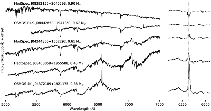
Figure 1: Five representative Praesepe and Hyades spectra obtained with the 2.4-m Hiltner telescope at MDM (Modspec and OSMOS spectrographs) and the MMT Observatory (Hectospec). Each spectrum is labeled with the instrument used, 2MASS designation of the target, and stellar mass $m$, and is normalized to the flux at 6555 Å. The right panel shows a close-up of the $\mathrm{H}\alpha$ line. The vertical dotted line indicates the center of the $\mathrm{H}\alpha$ line.

In Paper II, we presented new spectra for 130 Hyads and 390 Praesepe members obtained with the MDM Observatory 2.4-m Hiltner telescope and the WIYN 3.5-m telescope, both on Kitt Peak, AZ, and with the Magellan 6.5-m Clay telescope, Las Campanas Observatory, Chile. To these, we added archival spectra from Allen & Strom (1995), Stauffer et al. (1997a), and Kafka & Honeycutt (2004, 2006), and from the Sloan Digital Sky Survey (SDSS; York et al., 2000) archive. The resulting spectroscopic sample contained 720 spectra for 516 Praesepe members and 139 spectra for 130 Hyads.

3.1 New MDM Observations

We obtained additional spectra of Praesepe and Hyades stars over the course of 19 observing runs between 2014 Nov and 2023 Mar with the Modular Spectrograph (ModSpec) and the Ohio State Multi-Object Spectrograph (OSMOS) on the MDM Observatory 2.4-m Hiltner telescope (see Table 2). We configured ModSpec to have a wavelength coverage of 4500–7500 Å with $\approx$1.8 Å sampling and R $\approx$ 3600, which is the same configuration we used in Paper II.

With OSMOS, we used the blue 4K detector (OSMOS 4K) with a 1.2^′′ inner slit, for an approximate wavelength coverage of 4000–6800 Å, $\approx$0.7 Å sampling, R $\approx$ 9300, and peak efficiency at 6400 Å. We also used the red 4K detector (OSMOS R4K) with an OG-530 longpass filter and 1.2^′′ center slit, for an approximate wavelength coverage of 5500–10000 Å, $\approx$1.3 Å sampling, R $\approx$ 5000, and peak efficiency near 9000 Å.

MDM spectra obtained before 2021 were reduced with a script written in PyRAF, the Python-based command language for the Image Reduction and Analysis Facility (IRAF; Tody, 1986). Spectra obtained in 2021 and later were processed with the Python package PypeIt (Version 1.10.1.dev3+g52d10edd; Prochaska et al., 2020, 2020). We tested the agreement between the PyRAF and PypeIt pipelines by reducing a small sample of raw OSMOS images with both pipelines; most of these data were for stars with $\mathrm{H}\alpha$ absorption. We then measured the $\mathrm{H}\alpha$ equivalent width (see Section 6.1) in all spectra. The difference in measurements between the pipelines were $<$10%.

All the spectra were trimmed, overscan- and bias-corrected, cleaned of cosmic rays, flat-fielded, extracted, dispersion-corrected, and flux-calibrated. Excluding poor quality spectra (e.g., $S$/$N$ $\lesssim$ 5 or acquisition imperfections; 12% of Praesepe spectra and 8% of Hyades spectra), we collected 454 new spectra for 153 Praesepe members and 231 for 209 Hyads. The median $S$/$N$ for these spectra is 76 at $\mathrm{H}\alpha$.

Spectra for four stars observed at MDM are shown in Figure 1 for illustrative purposes. The MDM (and WIYN) spectra from Paper II and this work are available online.

3.2 New MMT Observations

We obtained additional spectra of Praesepe stars with the multiobject spectrograph Hectospec (Fabricant et al., 2005) on the MMT 6.5-m telescope, Mt. Hopkins, AZ. We used two fiber configurations over the course of two consecutive nights (2015 Nov 21-22). The first configuration was centered near $\alpha=08^{\mathrm{h}}41^{\mathrm{m}}10^{\mathrm{s}}$, $\delta=+20^{\circ}09^{\prime}59\farcs 1$ (J2000) and targeted 57 Praesepe stars. The second configuration was centered near $\alpha=08^{\mathrm{h}}41^{\mathrm{m}}36^{\mathrm{s}}$, $\delta=+19^{\circ}03^{\prime}50\farcs 5$ (J2000) and targeted 50 additional Praesepe stars.

We used the 600 line grating centered at 6300 Å, which results in an approximate wavelength coverage of 5030-7540 Å, and give $R\approx 11,000$ at $\mathrm{H}\alpha$. Our targets had 14.9 $<G<$ 19.7 mag, and our integration times were 3600 s (first night) and 5400 s (second night) with the first configuration, and 4500 s (second night) with the second configuration. After excluding spectra with $S$/$N$ $\lesssim$ 5, we have 126 MMT spectra for 47 Praesepe stars. The median $S$/$N$ at $\mathrm{H}\alpha$ is 48. All our MMT spectra are also available online.

The data were reduced automatically by the Smithsonian Astrophysical Observatory Telescope Data Center using the HSRED v2.0 pipeline. HSRED performs the basic reduction tasks: bias subtraction, flat-fielding, arc calibration, and sky subtraction. A Hectospec spectrum is included in Figure 1 for illustrative purposes. The MMT spectra are available online.3

Table 3: New Chandra Observations of Hyades Stars

Obs. ID	Nominal Aimpoint		Roll	Target(s)	Start	Duration
	$\alpha_{\rm J2000}$	$\delta_{\rm J2000}$	(°)	(Gaia DR3 Desig.)	Date	(s)
27553	03:18:15.13	+09:14.38.0	343.1	14143675198789504 (catalog Gaia DR3 14143675198789504)	2022-11	10085
27566	03:13:03.29	+32:53:55.2	210.1	125343573948444800 (catalog Gaia DR3 125343573948444800),	2022-11	10083
				125343608307015296 (catalog Gaia DR3 125343608307015296)
27572	04:38:56.73	+14:06:11.4	14.9	3309170875916905856 (catalog Gaia DR3 3309170875916905856)	2022-12	9902
27573	04:33:41.90	+19:00:38.0	28.5	3410453489022728576 (catalog Gaia DR3 3410453489022728576)	2022-12	9903
27574	04:32:40.40	+19:06:39.5	18.9	3410640887035452928 (catalog Gaia DR3 3410640887035452928),	2022-12	9903
				3410639993682264960 (catalog Gaia DR3 3410639993682264960)
27612	04:48:50.99	+15:56:57.9	299.8	3405127244241184256 (catalog Gaia DR3 3405127244241184256)	2022-12	10080
27622	05:30:14.19	+20:38:20.7	282.1	3402090466142958464 (catalog Gaia DR3 3402090466142958464)	2022-12	10083
27623	06:03:26.87	+24:02:26.8	265.5	3426209215771371648 (catalog Gaia DR3 3426209215771371648)	2022-12	20085
28490	06:50:34.35	$-$17:11:50.5	119.4	2946050323261707648 (catalog Gaia DR3 2946050323261707648)	2023-08	11082
29061	04:16:13.11	+18:53:04.2	91.2	47804394753757056, (catalog Gaia DR3 47804394753757056)	2023-11	9945
				47803952373768960 (catalog Gaia DR3 47803952373768960)
29076	04:28:40.63	+26:13:04.4	124.6	151222023217990016 (catalog Gaia DR3 151222023217990016)	2023-11	10086
29088	03:50:03.26	+22:35:43.0	268.0	64115585330656000 (catalog Gaia DR3 64115585330656000)	2023-12	10941
29111	04:47:09.56	+24:01:22.4	257.1	146989143968434688 (catalog Gaia DR3 146989143968434688)	2023-12	10086
29112	04:47:41.72	+26:09:11.2	244.1	154257259425702144 (catalog Gaia DR3 154257259425702144)	2023-12	10086

3.3 New Archival Spectroscopy

In Paper II, we found SDSS spectra for 66 Praesepe stars (as of 2013 Feb 14). We repeated this search using the SDSS Science Archive Server. SDSS spectra are sky-subtracted, corrected for telluric absorption, spectrophotometrically calibrated, and calibrated to heliocentric vacuum wavelengths. The wavelength coverage is 3800-9200 Å with R $\approx$ 4300 at $\mathrm{H}\alpha$. After excluding those with $S$/$N$ $\lesssim$ 5, we found SDSS spectra for 102 Praesepe stars and 16 Hyads (as of 2023 May 21).

We also searched for spectra in the the Large Sky Area Multi-Object Fiber Spectroscopic Telescope (LAMOST) Data Release 8 catalog. These spectra are flux- and wavelength-calibrated and sky-subtracted, and cover 3690-9100 Å with R $=1800$ at 5500 Å. After excluding those with $S$/$N$ $\lesssim$ 5, we found 873 LAMOST spectra for 324 Praesepe members and 535 for 252 Hyads. This includes 108 stars in Praesepe and 146 in the Hyades that did not have any previously available spectra.

Finally, J. Stauffer (2014, priv. comm.) shared 12 spectra of Hyads obtained as part of the Stauffer et al. (1997a) survey of the cluster. In Paper II we used 10 of these spectra to compare our equivalent width measurements to those of Stauffer et al. (1997a); here we include all 12 in our spectroscopic sample.

With our newly obtained spectra and newly found archival spectra, we now have a total of 2216 good quality (signal-to-noise ratio $S$/$N$ $\gtrsim$ 5) spectra for 879 Praesepe members; for the Hyades, the numbers are 943 and 565, respectively. Ninety-four of the Praesepe stars and 12 Hyads have five or more spectra.

4 X-ray data

Paper IV explains in detail the origin of the X-ray data for our Praesepe and Hyades stars. Briefly: we consolidated X-ray detections from the Röntgen Satellite (ROSAT), the Chandra X-ray Observatory (Chandra), the Neil Gehrels Swift Observatory (Swift), and the X-ray Multi-Mirror Mission Newton (XMM). For faint X-ray sources, we converted instrumental counts to unabsorbed energy fluxes $f_{\mathrm{X}}$ using WebPIMMS, and for bright X-ray sources, we performed spectral analyses to extract unabsorbed $f_{\mathrm{X}}$. For sources with flares in their X-ray light curves, we removed counts from the flare events before calculating $f_{\mathrm{X}}$ to obtain a more representative measurement of the quiescent X-ray activity level. We also homogenized all the fluxes to the 0.1–2.4 keV energy band.

Finally, for stars with more than one X-ray detection, we calculated the error-weighted average of the $f_{\mathrm{X}}$ values and adopted it as the bona fide unabsorbed $f_{\mathrm{X}}$ for that star. We include unabsorbed $f_{\mathrm{X}}$ values and their standard deviations (1$\sigma$ uncertainties) for Praesepe and Hyades stars in Columns 6 and 7 of Table 1.

Table 4: Overview of Columns in the Addendum to the Praesepe and Hyades X-ray Source Catalog

Column	Description
1	External catalog source ID
2	Provenance of X-ray information
3	IAU Name
4	Observation ID
5	Instrument
6, 7	R.A., Decl. for epoch J2000
8	X-ray positional uncertainty
9	Off-axis angle $\theta$
10	Detection likelihood $L$
11	Net counts in the broad band
12, 13	Net count rate and 1$\sigma$ uncertainty in broad band
14, 15	Net count rate and 1$\sigma$ uncertainty in soft band
16, 17	Net count rate and 1$\sigma$ uncertainty in hard band
18$-$20	Definition of broad, soft, and hard bands
21	Hardness ratio: (hard band $-$ soft band) /
	(hard band + soft band)
22	Exposure time
23	Variability flag: (0) no evidence for variability;
	(1) possibly variable; (2) definitely variable
24, 25	Unabsorbed energy flux and 1$\sigma$ uncertainty in the
	0.1–2.4 keV band
26	Source of energy flux: (ECF) from applying ECF;
	(SpecFit) from spectral fitting
27	X-ray flare removed?
28	Quality Flag
29	Name of the optical counterpart
30	Separation between X-ray source and optical counterpart

Note. — (This table is available in its entirety in machine-readable form.)

For this work, we updated our X-ray data to reflect developments since the publication of Paper IV, namely new Chandra observations, additions to the Chandra Source Catalog (CSC), and the thirteenth data release of the XMM EPIC Serendipitous Source Catalogue (4XMM-DR13; Webb et al., 2020).

As part of the Chandra Cool Targets program (Proposal 20201075, PI: Agüeros), we observed 17 Hyads with 14 pointings. The details of these observations are given in Table 3. For each observation, we used the ACIS-S3 chip in Very Faint telemetry mode. We processed the raw observations with the Chandra Interactive Analysis of Observations (CIAO; Fruscione et al., 2006) tools. We include in Table 4 the X-ray data for 13 of the targeted stars; four were undetected. We note that Table 4 in this work is an addendum to Table 3 in Paper IV.

In addition, two Hyads were added to the CSC following the release of version 2.1 starting in late 2022. Data for these two new X-ray detections are also included in Table 4.

Lastly, we found nine Praesepe low-mass members in 4XMM-DR13 that had no previous X-ray detections and one more that had ROSAT and Swift X-ray detections. We also found four Hyads with no previous X-ray detections, and four Hyads that only had a ROSAT X-ray detection. Data for these 18 4XMM-DR13 detections are included in Table 4.

5 Rotation Period Measurements

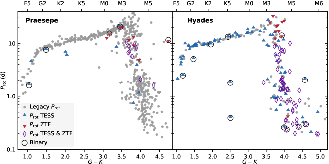
Figure 2: $P_{\mbox{\scriptsize rot}}$ vs. ($G-K$)  for Praesepe (left panel) and Hyades (right panel) stars. Gray circles indicate single stars with existing K2 $P_{\mbox{\scriptsize rot}}$ and other archival data collected in Rampalli et al. (2021) and Douglas et al. (2019) for Praesepe and the Hyades, respectively. Blue up triangles, red down triangles, and purple diamonds indicate stars with new $P_{\mbox{\scriptsize rot}}$ values from TESS, ZTF, or both, respectively. Black circles highlight new $P_{\mbox{\scriptsize rot}}$ values for known and candidate binaries.

The bulk of our rotational data for Praesepe and the Hyades came from the catalogs published in Rampalli et al. (2021) and Douglas et al. (2019), respectively. These catalogs consolidated $P_{\mbox{\scriptsize rot}}$ measurements made from light curves obtained by ground-based photometric surveys and by K2 (Howell et al., 2014). For Praesepe, we have 1052 members with these legacy $P_{\mbox{\scriptsize rot}}$ measurements; for the Hyades, the number is 233.

More recent observations of the two clusters with the Transiting Exoplanet Survey Satellite (TESS; Ricker et al., 2015), and continuing observations of the clusters with the Zwicky Transient Facility (ZTF; Masci et al., 2018), provided an opportunity to add to these totals. We showcase in Appendix A.1 the differing qualities of TESS and ZTF data and the benefit of using them together to extract more reliable rotation periods. Accordingly, we searched for light curves for stars in both clusters for which we have an optical spectrum and/or an X-ray detection.

Our procedure for TESS followed the strategy employed in a number of recent studies (e.g., McDivitt et al., 2022). We downloaded 40$\times$40 pixel cutouts from the available full frame images using TESScut (Brasseur et al., 2019), hosted by MAST. We extracted light curves for the pixel closest to each target using Casual Pixel Modeling (Wang et al., 2016) as implemented in the package unpopular (Hattori et al., 2022).

Using the interactive program tesscheck, we then inspected the TESS light curves for each star, selected the optimal subset of sectors to search for a rotational signature, and measured the period using Lomb–Scargle periodograms (Press & Rybicki, 1989). The visual inspection allowed us to catch uncorrected systematics that can introduce spurious signals into the periodogram and to flag and correct cases where the periodogram favors the half-period harmonic. We measured periods for 19 Praesepe stars and 125 Hyads using TESS data.

Our ZTF procedure used the approach developed by Curtis et al. (2020) to analyze Palomar Transient Factory (Law et al., 2010) data for the 2.7-Gyr-old cluster Ruprecht 147. We downloaded 8^′$\times$8^′ cutout images from IPAC (IRSA, 2022) and used simple aperture photometry to extract light curves for our targets and neighboring reference stars identified with Gaia. We corrected the light curves for systematics using the median-combined normalized light curves for reference stars. We inspected the resulting light curves, isolated the segment showing the cleanest periodic variability, and measured the period using Lomb–Scargle periodograms. We measured periods for 18 Praesepe stars and 59 Hyads using ZTF data.

In total, we have new $P_{\mbox{\scriptsize rot}}$ measurements for 28 Praesepe stars and 137 Hyads; 56 of these 165 stars have periods determined from both TESS and ZTF. For the Hyades, we have increased the sample of cluster members with known $P_{\mbox{\scriptsize rot}}$ by $\approx$50%, bringing the total to 370 stars. Figure 2 highlights our new $P_{\mbox{\scriptsize rot}}$ measurements against the background of legacy $P_{\mbox{\scriptsize rot}}$ for both clusters. In Table 1, we include the $P_{\mbox{\scriptsize rot}}$ data for Praesepe and Hyades members in Column 8, and we identify the source of the $P_{\mbox{\scriptsize rot}}$ measurement in Column 9.

We measured $P_{\mbox{\scriptsize rot}}$ = 0.39 d from the TESS data for 2MASS J05301288+2038486 (catalog ). This is an unusually short period for a star of its color; the other single stars with ($G-K$) $\approx$ 2.5 mag in Figure 2 have $P_{\mbox{\scriptsize rot}}$ between 10 and 20 d. As mentioned in Section 2, we found two Gaia DR3 sources within $<$2^′′ of each other and associated with this 2MASS source. Given this, we consider 2MASS J05301288+2038486 (catalog ) a candidate binary and flag it as such in Figure 2.

Figure 3 compares our TESS- and ZTF-derived $P_{\mbox{\scriptsize rot}}$ for the 56 cluster stars for which we have both. For 53 of the 56, the two $P_{\mbox{\scriptsize rot}}$ disagree by $<$4%. Of the three stars for which the disagreement is larger, two have TESS light curves that suggest multiple periods (see Appendix A.2). Indeed, for these two stars, 2MASS J02594633+3855363 (catalog ) and J04461522+1846294 (catalog 2MASS J04461522+1846294), the Gaia re-normalized unit weight error (RUWE) values are 5.0 and 3.4, respectively. As discussed in Paper IV, stars with RUWE $>$ 1.4 have a high probability of being unresolved binaries (e.g., Deacon & Kraus, 2020; Ziegler et al., 2020; Kervella et al., 2022). For these two stars, we adopted the TESS $P_{\mbox{\scriptsize rot}}$, assigned a binary flag = 1 (indicating they are candidate binaries), and flagged them as such in Figure 2.

For the third star, 2MASS J08412772+2103409 (catalog ), the TESS $P_{\mbox{\scriptsize rot}}$ (4.1 d) is the half harmonic of the ZTF $P_{\mbox{\scriptsize rot}}$ (8.2 d). We adopted the ZTF $P_{\mbox{\scriptsize rot}}$ for this star.

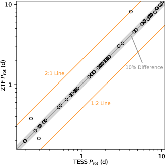
Figure 3: $P_{\mbox{\scriptsize rot}}$ from ZTF vs. $P_{\mbox{\scriptsize rot}}$ from TESS for the 56 Praesepe and the Hyades stars for which both surveys yielded periods. The gray line is the 1:1 relation, and the gray area the $\pm$10% difference range. The orange lines indicate the 1:2 and 2:1 harmonic lines. The two stars outside the 10% difference range have indications of multiple periodicity (see Appendix A); we adopted the TESS $P_{\mbox{\scriptsize rot}}$ and flag them as candidate binaries. For the star falling on the 2:1 harmonic line, we adopted the ZTF $P_{\mbox{\scriptsize rot}}$.

6 Other measurements and Derived Quantities

6.1 H$\alpha$ Equivalent Width Measurements

We measured the equivalent width (EW) of the $\mathrm{H}\alpha$ Balmer line in all our optical spectra, both newly acquired and archival (see Section 3). For this purpose, we used the tool PHEW (Núñez et al., 2022a), which automates the EW measurement using PySpecKit (Ginsburg & Mirocha, 2011) to fit a Voigt profile to the $\mathrm{H}\alpha$ line. We interactively defined continuum regions to either side of the $\mathrm{H}\alpha$ line in each spectrum, each between 5 and 35 Å in length.

PHEW performs 1000 Monte Carlo iterations by re-sampling the flux measurements within the flux uncertainties, or, if flux uncertainties are unavailable, by adding Gaussian noise to the flux spectrum. It then calculates the standard deviation of the 1000 EWs, which we adopted as the 1$\sigma$ EW uncertainty. We extracted the noise for each point from a Gaussian with width equal to the associated uncertainty at that point. If a flux spectrum lacked an associated uncertainty spectrum, we instead extracted the noise from a Gaussian with width equal to the standard deviation of the flux in the continuum regions defined for that spectrum.

If a star had multiple spectra available, we adopted the error-weighted mean EW (and the weighted mean standard error) as the representative EW value (and 1$\sigma$ uncertainty) for that star. Columns 10 and 11 in Table 1 include our measured EW and its 1$\sigma$ uncertainty, respectively. Negative EWs indicate emission, and an EW value of zero indicates that the spectrum for the star does not display a measurable $\mathrm{H}\alpha$ feature at that spectral resolution. Column 12 indicates the number of spectra we used to calculate each star’s EW value. The output figures from PHEW showing our EW measurements are available online.3

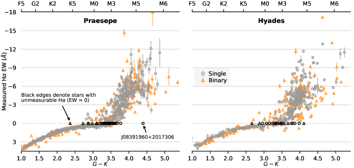
Figure 4: Measured $\mathrm{H}\alpha$ EW vs. ($G-K$) for Praesepe (left panel) and Hyades (right panel) members. Single stars are indicated with gray circles and binaries with orange triangles. Most of the EW error bars are smaller than the symbols. For clarity, we excluded from the right panel three outlier stars, one with ($G-K$) $>$ 5.5 mag and two with $\mathrm{H}\alpha$ EW $<-18$ Å. We also excluded stars with ($G-K$) $<$ 1.0 (spectral types earlier than $\approx$F5), as they are not relevant to our analysis. Black symbols indicate stars for which $\mathrm{H}\alpha$ is immeasurable in our spectra, and for which we set EW = 0. We consider one of these stars, annotated with its 2MASS designation, to be a potential non-member based on its unusual inactivity (see Section 6.1). The EWs shown here were not corrected for the quiescent $\mathrm{H}\alpha$ absorption present in these stars.

Figure 4 shows our EW measurements as a function of ($G-K$) for single and binary members (gray circles and orange triangles, respectively) of Praesepe (left panel) and of the Hyades (right panel). To better visualize the overall pattern, we omitted from the figure three Hyades outliers, one with ($G-K$) $>$ 5.5 mag and two with EW $<-18$ Å. We also excluded stars with ($G-K$) $<$ 1 (spectral type earlier than $\approx$F5) from the figure, as their lack of significant convective envelopes implies a different rotational evolution than the solar-like stars we focus on. However, we include in Table 1 values for all stars with at least one spectrum, regardless of spectral type.

In Figure 4, we also highlight with black symbols stars for which we find no measurable $\mathrm{H}\alpha$ (EW = 0 Å). Among these stars is 2MASS J08391960+2017306 (catalog ), a Praesepe star with ($G-K$) = 4.4 mag. All of its M5-M6 cousins exhibit some level of $\mathrm{H}\alpha$ emission, which makes its $\mathrm{H}\alpha$ inactivity unusual. In Paper IV, we considered this star a plausible Praesepe member based on its Kraus & Hillenbrand (2007) membership probability of $\approx$70%. However, none of the Gaia-based membership studies included in Paper IV considered it a cluster member, as its Gaia data do not include parallax and proper motion information (as of DR3). We therefore believe this star to be a likely contaminant in our membership catalog for Praesepe.

6.2 H$\alpha$ Relative to Quiescence

We corrected our measured EW values for each star to account for the quiescent photospheric $\mathrm{H}\alpha$ absorption naturally present in low-mass stars (cf. discussion for M dwarfs in Stauffer & Hartmann, 1986). As stars become more magnetically active, the line fills in and eventually transitions to emission. To report more accurately the level of chromospheric activity, we therefore need to consider this quiescent absorption level, which is a function of stellar mass $m$.

We used the empirical model of Newton et al. (2017), valid for stars with $m$ < 0.8 ${M_{\odot}}$, to calculate the quiescent photospheric absorption EW for cluster stars in that $m$ range. We then determined the relative EW by subtracting the quiescent EW from our measured EW. Column 13 in Table 1 indicates the relative EW value for each star with a measured EW and within the $m$ range of the empirical model.

6.3 The $\chi$ Factor and $L_{\mathrm{H}\alpha}$/$L_{\mathrm{bol}}$

To obtain $L_{\mathrm{H}\alpha}$/$L_{\mathrm{bol}}$ for stars with $\mathrm{H}\alpha$ in emission, we used the relation

$$\frac{L_{\mathrm{H}\alpha}}{L_{\mathrm{bol}}}=-\mathrm{EW}_{\mathrm{H}\alpha}\ \chi,$$ (1)

where EW${}_{\mathrm{H}_{\alpha}}$ is the relative $\mathrm{H}\alpha$ EW calculated in Section 6.2, and $\chi$ is the ratio of the continuum flux near the $\mathrm{H}\alpha$ line and of the apparent bolometric flux.

In Paper II, we presented several empirical $\chi$–photometric color relations based on PHOENIX ACES model spectra (Husser et al., 2013). We measured $\chi$ in the model spectra with surface gravity log($g$) = 5.0, solar metallicity, and in the effective temperature ($T_{\mathrm{eff}}$) range 2500–5200 K. For this work, we extended this calculation of $\chi$ to include the $T_{\mathrm{eff}}$ range 2300–6500 K by following the methodology described in Paper II (see Table 5).

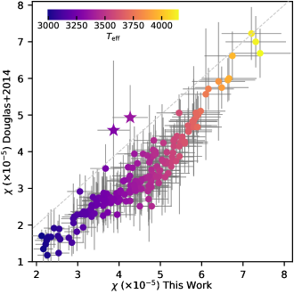
Figure 5: $\chi$ values for single Praesepe and Hyades stars calculated in Paper II vs. our calculations in this work, with their respective 1$\sigma$ errors. The gray dashed line is the 1:1 relation. Stars are color-coded according to their $T_{\mathrm{eff}}$ (as derived in this work; see Section 6.3), following the colorbar at the top left. The two stars represented with star symbols are objects for which we identified erroneous or unreliable $r^{\prime}$ photometry, which was used in Paper II to estimate their $\chi$.

To calculate $\chi$ for our cluster stars, we first derived their $T_{\mathrm{eff}}$ using the empirical $T_{\mathrm{eff}}$–$M_{G}$ relation of E. Mamajek. We linearly interpolated between the $M_{G}$ values in the empirical relation to obtain $T_{\mathrm{eff}}$. Columns 14 and 15 in Table 1 include our derived $T_{\mathrm{eff}}$ values and 1$\sigma$ uncertainties, respectively, for each main sequence cluster star.

Next, we calculated $\chi$ using $T_{\mathrm{eff}}$ by linearly interpolating between the $T_{\mathrm{eff}}$ values in Table 5. We assumed an intrinsic 10% error in our $T_{\mathrm{eff}}$–$\chi$ relation (identified in Paper II) and we added this error in quadrature to produce the 1$\sigma$ of the $\chi$ values we calculated for our cluster stars. Columns 16 and 17 include our $\chi$ values and 1$\sigma$ uncertainties for each cluster star. Lastly, we applied Equation 1 for all stars with relative $\mathrm{H}\alpha$ EW and $\chi$ values to obtain $L_{\mathrm{H}\alpha}$/$L_{\mathrm{bol}}$.

In Figure 5, we compare our new $\chi$ values to those in Paper II for the sample of single Praesepe and Hyades stars in both studies. The $\chi$ values from the earlier work were derived using the log($\chi$)–($r^{\prime}-K$) relation. We identified two stars for which an erroneous or unreliable $r^{\prime}$ photometry was assigned in Paper II (highlighted in Figure 5 with stars symbols), which explains their significant deviation from the general trend.

Our new $\chi$ values are systematically larger than those in Paper II by a factor of $\approx$1.3. This discrepancy is mostly driven by the $T_{\mathrm{eff}}$–($r^{\prime}-K$) relation in Paper II, which produces cooler $T_{\mathrm{eff}}$ values than those derived from the E. Mamajek table.

Table 5: $T_{\mathrm{eff}}$ and $\chi$ Values from PHOENIX Model Spectra

$T_{\mathrm{eff}}$	$\chi$	$T_{\mathrm{eff}}$	$\chi$	$T_{\mathrm{eff}}$	$\chi$
(K)	($\times 10^{-5}$)	(K)	($\times 10^{-5}$)	(K)	($\times 10^{-5}$)
6500	8.695	5000	9.581	3500	5.019
6400	8.797	4900	9.409	3400	4.477
6300	8.907	4800	9.279	3300	3.913
6200	9.038	4700	9.195	3200	3.328
6100	9.188	4600	9.127	3100	2.714
6000	9.299	4500	9.071	3000	2.181
5900	9.426	4400	8.658	2900	1.702
5800	9.510	4300	8.197	2800	1.252
5700	9.667	4200	7.632	2700	0.886
5600	9.777	4100	7.144	2600	0.618
5500	9.351	4000	6.825	2500	0.473
5400	8.961	3900	6.523	2400	0.603
5300	8.597	3800	6.201	2300	0.564
5200	9.160	3700	5.858
5100	9.622	3600	5.494

Note. — The methodology used to calculate $\chi$ is described in the appendix of Paper II.

6.4 Bolometric Luminosities and Rossby Numbers

We used the bolometric luminosities and $R_{\mathrm{o}}$ derived in Paper IV for our cluster stars. Briefly: to obtain $L_{\mathrm{bol}}$, we used the empirical log($L_{\mathrm{bol}}$)–$M_{G}$ relation of E. Mamajek.

To calculate $R_{\mathrm{o}}$, we first calculated $m$ using the empirical $m$–$M_{G}$ relation of E. Mamajek. Next, we found the convective turnover time $\tau$ using the empirical $m$–log($\tau$) relation of Wright et al. (2018). Finally, we computed $R_{\mathrm{o}}$ = $P_{\mbox{\scriptsize rot}}$/$\tau$.

In Paper II, we used the $m$–$M_{K}$ relation of Kraus & Hillenbrand (2007) to calculate $m$ and the $m$–log($\tau$) relation of Wright et al. (2011) to calculate $\tau$. Compared to the $R_{\mathrm{o}}$ values in Paper II, our new $R_{\mathrm{o}}$ values for the same stars are between 45% smaller and 20% larger, the median being 14% smaller. The largest discrepancies are mostly due to differences in the two $m$ calculation methods and to the distances used to calculate absolute magnitudes, as Paper II relied mostly on individual Hipparcos parallaxes or Hipparcos-derived cluster distances (van Leeuwen, 2009).

7 Results and Discussion

7.1 Chromospheric Activity

Figure 4 shows that in both clusters, all the late F, G, and K dwarfs have converged onto a tight sequence of $\mathrm{H}\alpha$ absorption (EW $>$ 0 Å), which is independent of magnetic activity. On the other hand, most M dwarfs exhibit some level of $\mathrm{H}\alpha$ emission. The transition between $\mathrm{H}\alpha$ absorption and emission in the two clusters occurs essentially at the same color (corresponding to a spectral type M0-M1), suggesting that both clusters are indeed of very similar ages.

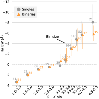
Figure 6: Color-binned median measured $\mathrm{H}\alpha$ EWs for single stars (gray circles) and binaries (orange triangles) in Praesepe and Hyades, with the 16^th and 84^th percentiles represented by whiskers

. The binary sample includes all stars with RUWE > 1.4. Numbers next to symbols indicate the number of stars in each bin.

Save for a handful of late K Hyads, the binaries in Figure 4 appear to follow the same distribution as their single-star counterparts in both clusters. To compare the two distributions more carefully, we binned our EWs by ($G-K$). Figure 6 shows the median EW values for single stars (gray circles) and binaries (orange triangles) in both Praesepe and the Hyades for 0.3 or 0.5 mag color bins, with their 16^th and 84^th percentiles represented by whiskers. The median EW values of single and binary stars are almost identical in most color bins, and the difference in median EW between single stars and binaries is $\buildrel<\over{\sim}$1$\sigma$ in all color bins.

We do note a slightly higher median $\mathrm{H}\alpha$ EW for binaries compared to single stars in the ($G-K$) = 3.0–3.3 mag bin (spectral types $\approx$M0–M2). However, these differences are not statistically significant, and we do not consider them to be evidence of enhanced chromospheric activity in binary systems in our sample. Lastly, the reddest color bin shows a $\approx$38% difference in median between single and binary stars. We attribute this discrepancy to the small sample size in those bins.

7.2 The Dependence of Chromospheric Activity on Rotation

To characterize the rotation–chromospheric activity relation, we followed previous authors in parametrizing the relation, in this case $R_{\mathrm{o}}$–$L_{\mathrm{H}\alpha}$/$L_{\mathrm{bol}}$, as a flat region connected to a power-law. For stars with $R_{\mathrm{o}}$ $\leq{R_{\mathrm{o}}}_{\mathrm{,sat}}$, activity is saturated—i.e., constant—and equal to ($L_{\mathrm{H}\alpha}$/$L_{\mathrm{bol}}$)_sat. Above ${R_{\mathrm{o}}}_{\mathrm{,sat}}$, activity declines as a power-law with index $\beta$, and is, therefore, unsaturated. Functionally, this corresponds to

$$\frac{L_{\mathrm{H}\alpha}}{L_{\mathrm{bol}}}=\left\{\begin{array}[]{l l}\left(\frac{L_{\mathrm{H}\alpha}}{L_{\mathrm{bol}}}\right)_{\mathrm{sat}}&\quad\textrm{if $R_{\mathrm{o}}\leq R_{\mathrm{o,sat}}$}\\ CR_{\mathrm{o}}^{\beta}&\quad\textrm{if $R_{\mathrm{o}}$ > $R_{\mathrm{o,sat}}$}\end{array}\right.$$ (2)

where $C$ is a constant. This model has been widely used in the literature (e.g., Randich 2000, Wright et al. 2011, Paper II, Núñez et al. 2015, Paper IV).

Table 6: Rotation–Activity Relation Fitting Results

	$R_{\mathrm{o}}$–$L_{\mathrm{H}\alpha}$/$L_{\mathrm{bol}}$				$R_{\mathrm{o}}$–$L_{\mathrm{X}}$/$L_{\mathrm{bol}}$
Sample	$N_{\star}$	($L_{\mathrm{H}\alpha}$/$L_{\mathrm{bol}}$)sat	$R_{\mathrm{o,sat}}$	$\beta$	$N_{\star}$	$\beta_{\mathrm{sup}}$	$R_{\mathrm{o,sup}}$	($L_{\mathrm{X}}$/$L_{\mathrm{bol}}$)sat	$R_{\mathrm{o,sat}}$	$\beta$
		($10^{-4}$)						($10^{-3}$)
Single stars
Praesepe	196	1.76$\pm$0.09	0.28${}^{+0.02}_{-0.03}$	$-5.19^{+1.32}_{-0.94}$	124	0.70${}^{+0.60}_{-0.32}$	0.011$\pm$0.005	1.14$\pm$0.12	0.19$\pm$0.02	$-3.48^{+0.34}_{-0.39}$
Hyades	116	1.53$\pm$0.08	0.31${}^{+0.01}_{-0.02}$	$-7.07^{+1.40}_{-1.57}$	162	0.54${}^{+0.19}_{-0.15}$	0.014${}^{+0.004}_{-0.005}$	1.15${}^{+0.13}_{-0.12}$	0.17$\pm$0.02	$-3.04^{+0.27}_{-0.28}$
All	312	1.65$\pm$0.06	0.29$\pm$0.01	$-5.85^{+0.81}_{-0.80}$	286	0.53${}^{+0.16}_{-0.12}$	0.015${}^{+0.003}_{-0.005}$	1.17$\pm$0.09	0.17$\pm$0.01	$-3.18^{+0.20}_{-0.21}$
Binaries & stars with RUWE $>$ 1.4
Praesepe	134	1.84${}^{+0.11}_{-0.12}$	0.24$\pm$0.03	$-2.77^{+0.51}_{-0.70}$	112	0.13${}^{+0.22}_{-0.11}$	0.009${}^{+0.007}_{-0.004}$	1.17$\pm$0.15	0.12${}^{+0.03}_{-0.02}$	$-2.20^{+0.26}_{-0.38}$
Hyades	92	1.63$\pm$0.14	0.16${}^{+0.05}_{-0.04}$	$-1.51^{+0.39}_{-0.59}$	138	0.08${}^{+0.15}_{-0.07}$	0.009${}^{+0.007}_{-0.005}$	1.02${}^{+0.11}_{-0.10}$	0.14$\pm$0.02	$-2.36^{+0.27}_{-0.31}$
All	226	1.76$\pm$0.09	0.20${}^{+0.03}_{-0.04}$	$-2.05\pm$0.50	250	0.06${}^{+0.11}_{-0.05}$	0.009${}^{+0.007}_{-0.005}$	1.07$\pm$0.08	0.13${}^{+0.02}_{-0.01}$	$-2.26^{+0.19}_{-0.24}$

We used the open-source Markov-chain Monte Carlo (MCMC) package emcee (Foreman-Mackey et al., 2013) to fit this three-parameter model to our data. Following the emcee implementation by Magaudda et al. (2020), we allowed for a nuisance parameter $f$ to account for underestimated errors. We assumed flat priors over each parameter and used 300 walkers, each taking 5000 steps in their MCMC chain, to infer maximum likelihood parameters. Our results are presented in Figure 7 for several subsamples. The posterior distributions for each parameter and 2D correlations between pairs of parameters from each fit are included in a figure set in Appendix B; 200 random samples from these distributions are shown in Figure 7, along with the maximum a posteriori model.

In Table 6, we present the ($L_{\mathrm{H}\alpha}$/$L_{\mathrm{bol}}$)_sat, $R_{\mathrm{o}}$_,sat, and $\beta$ parameters corresponding to the maximum a posteriori model for the six subsamples we show in Figure 7, and we also annotate them in each panel in the Figure. For each parameter, we assumed the 50^th percentile of the results to be the mean value, and the 16^th and 84^th percentiles, their approximate 1$\sigma$ uncertainties. In all cases, the nuisance parameter $f$ converged to $\approx$0.06, suggesting that our $L_{\mathrm{H}\alpha}$/$L_{\mathrm{bol}}$ uncertainties are underestimated by no more than $\approx$6%.

We applied the model in Equation 2 to single members separately from binary members and members with RUWE $>$ 1.4. Without a more detailed study of the characteristics of the known and candidate binaries, it is not possible to determine whether gravitational and magnetic interactions may have altered their spin-down evolution. Furthermore, for binaries, the $\chi$ and $\tau$ parameters—ultimately derived from $M_{G}$ and used to calculate $L_{\mathrm{H}\alpha}$/$L_{\mathrm{bol}}$ and $R_{\mathrm{o}}$, respectively—have dubious validity, as we expect them to be overestimated to varying degrees for binaries, the effects of which are difficult to track in our analysis. In our discussion below, we therefore distinguish between the nominally single stars and those flagged as either known or candidate binaries.

We also applied the model to members of each cluster separately and together. Combining the stars from both clusters to create a larger sample is reasonable given the very similar ages and metallicities of Praesepe and the Hyades (e.g., Cummings et al., 2018; Gaia Collaboration et al., 2018b; Douglas et al., 2019). We consider the results from the combined sample, which we nicknamed HyPra, to be most statistically meaningful. In any case, the values for the parameters obtained from applying the model to the clusters individually almost always agree to within 1$\sigma$ (and always to within 2$\sigma$).

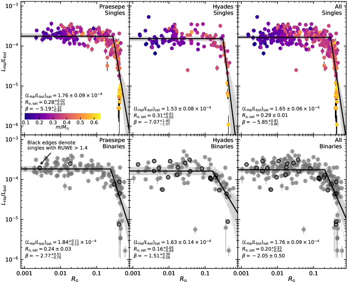
Figure 7: $L_{\mathrm{H}\alpha}$/$L_{\mathrm{bol}}$ vs. $R_{\mathrm{o}}$ for Praesepe stars (left panels), for Hyads (middle), and for the two clusters combined (right). The top panels show single stars, and the bottom panels show confirmed and candidate binaries. This latter set includes nominally single stars with RUWE $>$ 1.4 (indicated with solid black circles). Single stars are color-coded by their $m$ according to the colorbar in the top left panel. The solid black line in each panel is the maximum a posteriori fit from the MCMC algorithm, and the gray lines are 200 random samples from the posterior probability distributions. We assumed a flat saturated regime described by ($L_{\mathrm{H}\alpha}$/$L_{\mathrm{bol}}$)_sat and $R_{\mathrm{o}}$_,sat, and an unsaturated regime described by a power-law of index $\beta$. The results of the fit for these three parameters are given in each panel. We show in Appendix B the marginalized posterior probability distributions from the MCMC analysis for each fit.

The Saturated Regime

For single HyPra stars, ($L_{\mathrm{H}\alpha}$/$L_{\mathrm{bol}}$)_sat = (1.65$\pm$0.06)$\times$10^-4, with only a handful of outliers in the Hyades deviating from the narrow distribution around this $L_{\mathrm{H}\alpha}$/$L_{\mathrm{bol}}$ level (see top panels, Figure 7). This value of ($L_{\mathrm{H}\alpha}$/$L_{\mathrm{bol}}$)_sat is consistent with what Newton et al. (2017) found for their sample of saturated field M dwarfs, for which $L_{\mathrm{H}\alpha}$/$L_{\mathrm{bol}}$ = (1.49$\pm$0.08)$\times$10^-4, within 2$\sigma$ of our result.

On the other hand, in Paper II, we found that, for single members in both clusters, ($L_{\mathrm{H}\alpha}$/$L_{\mathrm{bol}}$)_sat = (1.26$\pm$0.04)$\times$10^-4. Similarly, Núñez et al. (2017) found ($L_{\mathrm{H}\alpha}$/$L_{\mathrm{bol}}$)_sat = (1.27$\pm$0.02)$\times$10^-4 for single members of the $\approx$500 Myr-old cluster M37. Both of these values are statistically discrepant with our new result at the $\approx$4$\sigma$ level. However, in neither of these studies were the EW measurements corrected to account for the quiescent photospheric $\mathrm{H}\alpha$ absorption. In addition, our new $\chi$ values used to calculate $L_{\mathrm{H}\alpha}$/$L_{\mathrm{bol}}$ are $\approx$1.3$\times$ larger than those used in the two studies (see Section 6.3).

Accounting for quiescent absorption and using updated larger $\chi$ values results in slightly enhanced $L_{\mathrm{H}\alpha}$/$L_{\mathrm{bol}}$ values, which explains our larger best-fit value for ($L_{\mathrm{H}\alpha}$/$L_{\mathrm{bol}}$)_sat compared to Paper II and Núñez et al. (2017). In Appendix C, we repeated our fitting to the $R_{\mathrm{o}}$–$L_{\mathrm{H}\alpha}$/$L_{\mathrm{bol}}$ data when the EW data are not corrected, which provides a clearer comparison to previous studies that did not apply any correction to the EW values.

Binaries and stars with RUWE $>$ 1.4 (bottom panels, Figure 7) exhibit a spread around the saturated level similar to that observed in single cluster stars. Their ($L_{\mathrm{H}\alpha}$/$L_{\mathrm{bol}}$)_sat value, (1.76$\pm$0.09)$\times$10^-4, is within 1$\sigma$ of that of their single counterparts.

The Rossby Threshold Between Saturated and Unsaturated Regimes

For single HyPra stars, the transition between the saturated and unsaturated regimes occurs at $R_{\mathrm{o}}$_,sat = 0.29$\pm 0.01$. We note that the quoted 1$\sigma$ uncertainties for $R_{\mathrm{o}}$_,sat in all of the studies under consideration, including this one, are unrealistically small, as $R_{\mathrm{o}}$ uncertainties are difficult to estimate and therefore not included when running the MCMC fit. As such, we do not expect our result to statistically agree with results in similar studies. Indeed, Newton et al. (2017) found $R_{\mathrm{o}}$_,sat = 0.21$\pm 0.02$, Paper II, 0.11${}^{+0.02}_{-0.03}$, and Núñez et al. (2017), 0.03$\pm 0.01$. All of these results are statistically discrepant by $\geq$3$\sigma$.

As we show in Appendix C, however, re-running our MCMC fit without applying the quiescent absorption correction to our measured EW values results in $R_{\mathrm{o}}$_,sat values that do agree statistically with that from Paper II, but are still statistically discrepant from that in Núñez et al. (2017).

Lastly, for known and candidate binaries, $R_{\mathrm{o}}$${}_{\mathrm{,sat}}=0.20^{+0.03}_{-0.04}$, which is within 2$\sigma$ of the value of single members, notwithstanding the unaccounted for uncertainties in $R_{\mathrm{o}}$ mentioned above.

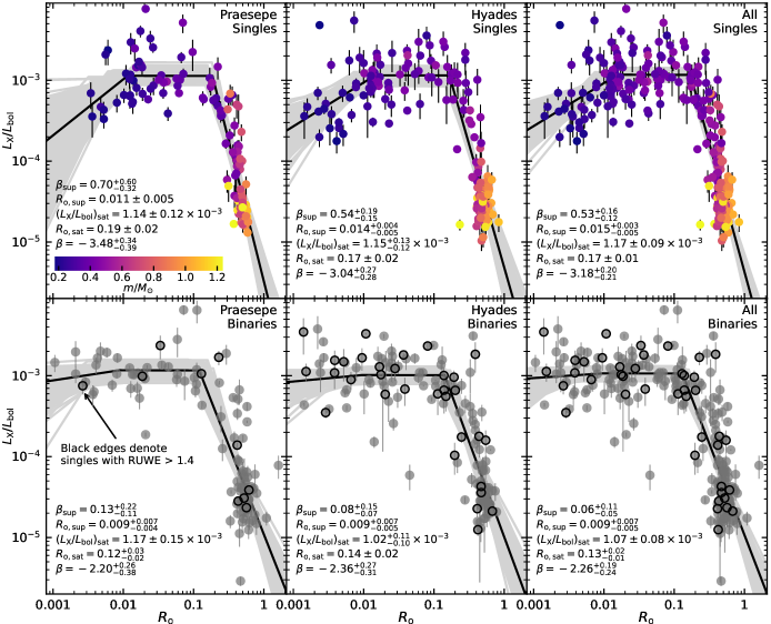
Figure 8: Same as Figure 7, but for $L_{\mathrm{X}}$/$L_{\mathrm{bol}}$. In addition to the saturated and unsaturated regimes in Figure 7, we also assumed the existence of a supersaturated regime described by a power-law of index $\beta_{\mathrm{sup}}$ and $R_{\mathrm{o}}$_,sup. The result of the fit for the five parameters $\beta_{\mathrm{sup}}$, $R_{\mathrm{o}}$_,sup, ($L_{\mathrm{X}}$/$L_{\mathrm{bol}}$)_sat, $R_{\mathrm{o}}$_,sat, and $\beta$, are given in each panel. We show in Appendix B the marginalized posterior probability distributions from the MCMC analysis for each fit.

The Unsaturated Regime

For single HyPra stars, we found that $\beta=-5.85^{+0.81}_{-0.80}$. This result is $>$4$\sigma$ away from that of Newton et al. (2017), who found $\beta=-1.7$$\pm$$0.1$. Although our methods are similar to those used by these authors, our unsaturated stars are significantly different from those in Newton et al. (2017) in three ways.

First, the majority of stars with $R_{\mathrm{o}}$ $>$ $R_{\mathrm{o}}$_,sat in our sample have masses $\gtrsim$0.5 ${M_{\odot}}$ (see the colormap in Figure 7), whereas their sample does not have any stars with masses $\gtrsim$0.5 ${M_{\odot}}$ (see their Figure 6). Second, our largest $R_{\mathrm{o}}$ values are $\approx$ 0.5, whereas most unsaturated stars in their sample have $R_{\mathrm{o}}$ $>$ 0.5 and up to 2.0. And third, all of our stars are $\approx$700 Myr old, whereas their sample mostly included field-age dwarfs, which presumably have ages $>>$1 Gyr. The $\beta$ discrepancy between these two samples may partly be evidence for a steeper decay in chromospheric activity for the more massive, partly convective dwarfs versus for fully or almost fully convective dwarfs. On the other hand, the $\beta$ discrepancy may just reflect different dominant chromospheric radiative coolants for stars at different $T_{\mathrm{eff}}$: in M dwarfs, Balmer lines emission dominates, whereas in G and K dwarfs, Ca ii and Mg ii emission dominates (Linsky et al., 1982; Reid & Hawley, 2005).

In Paper II, we found that $\beta=-0.73^{+0.16}_{-0.12}$, and in Núñez et al. (2017), $\beta=-0.51$$\pm$$0.02$. Both of these results are also statistically inconsistent with our new result. However, as noted earlier, these two studies must be compared to our results when we do not apply the quiescent correction to our EWs (see Appendix C).

For binaries and candidate binaries, we found that $\beta=-2.05$$\pm$$0.50$, which is within 3$\sigma$ of our result for single stars. The shallower $\beta$ for binaries partly reflects the slightly higher—although statistically insignificant—$\mathrm{H}\alpha$ emission in binaries compared to single stars in the ($G-K$) = 3.0–3.3 mag bin ($\approx$M0–M2 stars; see Figure 6).

However, as we mentioned earlier, using $M_{G}$ to derive $T_{\mathrm{eff}}$ and $m$, from which we then calculated $\chi$ and $\tau$, leads to overestimated $L_{\mathrm{H}\alpha}$/$L_{\mathrm{bol}}$ and $R_{\mathrm{o}}$ values to varying degrees for binaries. Therefore, we do not consider our shallower $\beta$ result to be evidence for higher chromospheric activity in unsaturated binaries compared to their single counterparts.

7.3 The Dependence of Coronal Activity on Rotation

In Paper IV, we presented a comprehensive study of $L_{\mathrm{X}}$/$L_{\mathrm{bol}}$ as a coronal activity indicator and of its dependence on $R_{\mathrm{o}}$ in Praesepe and the Hyades. We used a sample of 114 Praesepe and 63 Hyades single stars to characterize the saturated and unsaturated regimes in the $R_{\mathrm{o}}$–$L_{\mathrm{X}}$/$L_{\mathrm{bol}}$ plane, using the same parametrization given in Equation 2 (we also had 107 Praesepe and 98 Hyades binary stars or with RUWE $>$ 1.4).

In that study, we found weak evidence for supersaturation (see appendix B of Paper IV), the $R_{\mathrm{o}}$ regime in which super-fast rotators ($R_{\mathrm{o}}$ $\lesssim$ 0.01) show a decrease in activity level relative to their saturated cousins. To characterize this behavior, we modified the $R_{\mathrm{o}}$–$L_{\mathrm{X}}$/$L_{\mathrm{bol}}$ relation parametrization presented in Equation 2 by adding a secondary power-law at small $R_{\mathrm{o}}$: below $R_{\mathrm{o,sup}}$, activity declines as a power-law with index $\beta_{\mathrm{sup}}$.

Since that study, we have added 154 stars to our sample of cluster stars with both $R_{\mathrm{o}}$ and $L_{\mathrm{X}}$/$L_{\mathrm{bol}}$ measurements. These are primarily Hyads; we have an additional 99 single stars and 40 known and candidate binaries in that cluster with these measurements (the numbers for Praesepe are 10 and five, respectively). Figure 8 shows the updated $R_{\mathrm{o}}$–$L_{\mathrm{X}}$/$L_{\mathrm{bol}}$ relation for single stars (top panels) and binary stars (bottom panels) for Praesepe (left panels), Hyades (middle panels), and both clusters combined (right panels).

With this update, we found more compelling evidence of supersaturation in single stars in both clusters. In this regime, single stars in Praesepe follow a power-law of slope $\beta_{\mathrm{sup}}=0.70^{+0.60}_{-0.32}$, 2$\sigma$ away from a flat relation, while in Hyades, where the number of supersaturated stars is larger, $\beta_{\mathrm{sup}}=0.54^{+0.19}_{-0.15}$, 3$\sigma$ away from being flat. Meanwhile, for the combined HyPra sample $\beta_{\mathrm{sup}}=0.53^{+0.16}_{-0.12}$, which is at least 4$\sigma$ away from a flat relation (top row, Figure 8).

On the other hand, for known and candidate binaries, the supersaturated regime is almost indistinguishable from a flat relation ($\beta_{\mathrm{sup}}$ = 0) and $R_{\mathrm{o}}$_,sup remains poorly constrained (bottom panels, Figure 8). The lack of supersaturation in binaries may be partly explained by magnetic interactions between the binary components increasing their quiescent activity levels and/or increasing the frequency of flaring activity. The updated results for the other four parameters, namely, $R_{\mathrm{o}}$_,sup, ($L_{\mathrm{X}}$/$L_{\mathrm{bol}}$)_sat, $R_{\mathrm{o}}$_,sat, and $\beta$, only change marginally compared to our results in Paper IV, with $\beta$ being now more constrained for both single and binary members. We include these updated parameters in Table 6.

7.4 Chromospheric Versus Coronal Activity

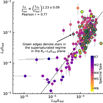
Figure 9: $L_{\mathrm{X}}$/$L_{\mathrm{bol}}$ vs. $L_{\mathrm{H}\alpha}$/$L_{\mathrm{bol}}$ for single stars in Praesepe and the Hyades, color-coded by their spectral type. The dashed black line is the power-law relation found with a least-squares bisector regression. The slope and Pearson $r$ of the regression is noted at the top left. Green edges highlight stars in the supersaturated regime in the $R_{\mathrm{o}}$–$L_{\mathrm{X}}$/$L_{\mathrm{bol}}$ plane.

Several studies have shown differences in the dependence of $\mathrm{H}\alpha$ and X-ray emission on rotation (e.g., Hodgkin et al., 1995; Núñez et al., 2017; Preibisch & Feigelson, 2005; Stelzer et al., 2013). These differences could point to differences in magnetic heating mechanisms acting on different layers of the stellar atmospheres. At the same time, some positive correlation between $L_{\mathrm{X}}$/$L_{\mathrm{bol}}$ and $L_{\mathrm{H}\alpha}$/$L_{\mathrm{bol}}$ is expected, partly because a fraction of the coronal X-rays will inevitably heat the underlying chromosphere (Mullan, 1976; Cram, 1982). We directly compare $L_{\mathrm{X}}$/$L_{\mathrm{bol}}$ and $L_{\mathrm{H}\alpha}$/$L_{\mathrm{bol}}$ for single stars in both clusters in Figure 9 to characterize their relationship.

Using a least-squares bisector regression, we found a power-law relation such that $L_{\mathrm{X}}$/$L_{\mathrm{bol}}$ $\propto$ ($L_{\mathrm{H}\alpha}$/$L_{\mathrm{bol}}$)^α, with $\alpha$ = 1.23$\pm 0.09$ (dashed line, Figure 9), with a correlation coefficient $r$ = 0.77, which suggests a strong positive correlation between $L_{\mathrm{X}}$/$L_{\mathrm{bol}}$ and $L_{\mathrm{H}\alpha}$/$L_{\mathrm{bol}}$.

Most of the stars are concentrated near $L_{\mathrm{H}\alpha}$/$L_{\mathrm{bol}}$ $\approx~{}10^{-4}$ and $L_{\mathrm{X}}$/$L_{\mathrm{bol}}$ $\approx 10^{-3}$. These two values correspond to the saturation levels in both activity indicators. The tail-like structure that goes from this locus to smaller values in both $L_{\mathrm{H}\alpha}$/$L_{\mathrm{bol}}$ and $L_{\mathrm{X}}$/$L_{\mathrm{bol}}$ corresponds to stars in the unsaturated regime of both indicators. Finally, we highlight in Figure 9 stars in the supersaturated regime in the $R_{\mathrm{o}}$-$L_{\mathrm{X}}$/$L_{\mathrm{bol}}$ plane, most of which lie below the power-law relation.

In Núñez et al. (2017), we found for single members of M37 a weaker correlation ($r$ = 0.63) and a slope closer to 1:1 ($\alpha$ = 1.05$\pm$0.01). In that $\approx$500-Myr-old cluster, our sample included stars in the spectral range K0–M1 that were almost all saturated in both $L_{\mathrm{H}\alpha}$/$L_{\mathrm{bol}}$ and $L_{\mathrm{X}}$/$L_{\mathrm{bol}}$. By contrast, our Praesepe and Hyades sample includes K6–M6 stars with $L_{\mathrm{H}\alpha}$/$L_{\mathrm{bol}}$ and $L_{\mathrm{X}}$/$L_{\mathrm{bol}}$ measurements (see the colorbar in Figure 9), and a significant number of these are unsaturated. In addition, the $L_{\mathrm{H}\alpha}$/$L_{\mathrm{bol}}$ values in Núñez et al. (2017) did not account for the quiescent correction described in Section 6.2, the effect of which is difficult to quantify in this analysis.

By contrast, He et al. (2019) found $\alpha$ = 1.12$\pm$0.30 for a sample of field-age K and M dwarfs. This result agrees with ours at the 1$\sigma$ level. Also, for a sample of M dwarfs within 10 pc, Stelzer et al. (2013) found $\alpha$ = 1.90$\pm$0.31, implying a steeper slope for the unsaturated rotation–activity relation—but this value is in 2$\sigma$ agreement with our value for $\alpha$. The former study accounted for quiescent $\mathrm{H}\alpha$ absorption, while the latter did not.

It is more informative to directly compare relations for $L_{\mathrm{H}\alpha}$/$L_{\mathrm{bol}}$ and $L_{\mathrm{X}}$/$L_{\mathrm{bol}}$ as a function of $R_{\mathrm{o}}$. We re-create the top right panel of Figures 7 and 8, i.e., the HyPra sample, as the top and bottom panels (respectively) in Figure 10. We highlight the results from the MCMC algorithm with solid lines and shaded regions, corresponding to the maximum a posteriori and 1$\sigma$ MCMC results. We also highlight with vertical dashed lines the threshold Rossby values, namely, $R_{\mathrm{o}}$_,sat for the $R_{\mathrm{o}}$–$L_{\mathrm{H}\alpha}$/$L_{\mathrm{bol}}$ relation and $R_{\mathrm{o}}$_,sup and $R_{\mathrm{o}}$_,sat for the $R_{\mathrm{o}}$–$L_{\mathrm{X}}$/$L_{\mathrm{bol}}$ relation.

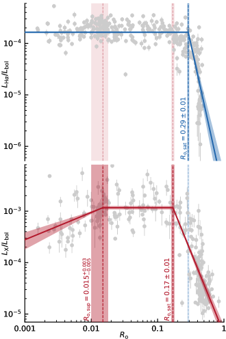
Figure 10: $L_{\mathrm{H}\alpha}$/$L_{\mathrm{bol}}$ vs. $R_{\mathrm{o}}$ (top panel) and $L_{\mathrm{X}}$/$L_{\mathrm{bol}}$ vs. $R_{\mathrm{o}}$ (bottom panel) for single members of Praesepe and the Hyades combined (gray circles). The maximum a posteriori fits from the MCMC algorithm (see Sections 7.2 and 7.3) and their approximate 1$\sigma$ uncertainties are indicated with solid lines and shaded regions, respectively. The Rossby threshold values ($R_{\mathrm{o}}$_,sup and $R_{\mathrm{o}}$_,sat) and their 1$\sigma$ uncertainties are indicated with vertical dashed lines and shaded regions, respectively, and are annotated next to each line. We extend these vertical dashed lines along both panels to more easily compare the different regimes (supersaturated, saturated, and unsaturated) in both chromospheric ($L_{\mathrm{H}\alpha}$/$L_{\mathrm{bol}}$) and coronal ($L_{\mathrm{X}}$/$L_{\mathrm{bol}}$) activity indicators.

In the top panel of Figure 10 the lack of supersaturation in $L_{\mathrm{H}\alpha}$/$L_{\mathrm{bol}}$ is evident. If the fastest spinners ($R_{\mathrm{o}}$ $\lesssim$ 0.01) appear supersaturated in X-rays but not in $\mathrm{H}\alpha$, then whatever mechanism is curtailing the magnetically driven X-ray emission is present in the coronae of these stars, but not in their chromospheres.

Of the two most invoked mechanisms to explain supersaturation, centrifugal stripping of the corona (Jardine & Unruh, 1999) and reduction of the filling factor (Stȩpień et al., 2001), our evidence favors the former, echoing the conclusions of, e.g., Marsden et al. (2009); Jackson & Jeffries (2010); Wright et al. (2011). In the centrifugal stripping scenario, the chromospheric layers would not be affected by the stars’ super rapid rotation, whereas in the reduced filling factor scenario, all atmospheric layers would be impacted. The centrifugal stripping scenario would not conflict with the expectation that some of the chromospheric heating comes from X-rays emitted in the corona. It is reasonable to expect that most of the X-rays heating the chromosphere originate in the denser inner layers of the corona. Thus, it is possible for $L_{\mathrm{X}}$/$L_{\mathrm{bol}}$ to decrease due to plasma loss at the outermost layers of the corona, while maintaining $L_{\mathrm{H}\alpha}$/$L_{\mathrm{bol}}$ mostly unaffected.

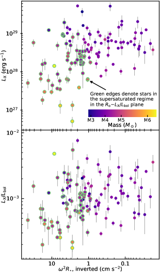
Figure 11: $L_{\mathrm{X}}$ (top panel) and $L_{\mathrm{X}}$/$L_{\mathrm{bol}}$ (bottom panel) vs. centrifugal acceleration for single members of Praesepe and the Hyades that are in the saturated or supersaturated regimes in the top right panel of Figure 8. Stars are color coded by their spectral type. Green edges highlight stars in the supersaturated regime in the $R_{\mathrm{o}}$–$L_{\mathrm{X}}$/$L_{\mathrm{bol}}$ plane. The x axis is inverted (i.e., acceleration increases toward the left) for easier comparison to Figure 8.

As an additional test of whether we are seeing evidence of centrifugal stripping, we compared X-ray activity to the stellar centrifugal acceleration, defined as the square of the angular rotation frequency (i.e., the reciprocal of $P_{\mbox{\scriptsize rot}}$) times the stellar radius: $\omega^{2}R_{\mathrm{\star}}$. We derived $R_{\mathrm{\star}}$ and 1$\sigma$ uncertainties for main sequence cluster stars using the empirical $R_{\mathrm{\star}}$–$M_{G}$ relation of E. Mamajek, and they are included in Table 1. In Figure 11 we plot $L_{\mathrm{X}}$ and $L_{\mathrm{X}}$/$L_{\mathrm{bol}}$ vs. centrifugal acceleration for Praesepe and Hyades single members with $R_{\mathrm{o}}$ $<$ $R_{\mathrm{o}}$_,sat, and we highlight with green circles those stars with $R_{\mathrm{o}}$ $<$ $R_{\mathrm{o}}$_,sup. We find all stars in the supersaturated regime to have $\omega^{2}R_{\mathrm{\star}}$ $\buildrel>\over{\sim}$ 1 cm s^-2. We see an indication of supersaturation at $\omega^{2}R_{\mathrm{\star}}$ $\buildrel>\over{\sim}$ 3 cm s^-2, although not as clear as in the $L_{\mathrm{X}}$/$L_{\mathrm{bol}}$–$R_{\mathrm{o}}$ plane.

Also evident in Figure 10 is the smaller $R_{\mathrm{o}}$_,sat for $L_{\mathrm{X}}$/$L_{\mathrm{bol}}$ compared to $L_{\mathrm{H}\alpha}$/$L_{\mathrm{bol}}$—6$\sigma$ away from each other. This difference indicates that the transition from the saturated to unsaturated regimes does not occur in tandem in these two layers of the stellar atmosphere. Our HyPra sample suggests that as stars spin down (i.e., their $R_{\mathrm{o}}$ increases), saturation ends in the corona before it ends in the chromosphere. This difference in timing could indicate a difference in the sensitivity to field components of the magnetic field at different atmospheric altitudes, which would not be surprising. For example, See et al. (2019) found that $R_{\mathrm{o}}$_,sat for an activity indicator derived from Zeeman-Doppler imaging, which is particularly sensitive to large-scale components of the magnetic field (e.g. Brown et al., 1991), is smaller than that of other activity indicators. Based on our results, we infer that $L_{\mathrm{X}}$/$L_{\mathrm{bol}}$ is more sensitive to large-scale components than $L_{\mathrm{H}\alpha}$/$L_{\mathrm{bol}}$.

8 Conclusion

We have performed an analysis of chromospheric and coronal activity in low-mass stars in the Praesepe and Hyades open clusters. These two coeval groups of stars, with a crucial age between that of very young clusters and that of field stars, are pivotal in our understanding of the dependence of stellar magnetic activity on rotation and of the evolution of this dependence.

We used the Praesepe and Hyades membership catalogs of Paper IV, which include several stellar parameters such as mass, distance, $L_{\mathrm{bol}}$, $P_{\mbox{\scriptsize rot}}$, $\tau$, and binarity identification, as well as Gaia and 2MASS photometry. We updated these quantities when appropriate (e.g., to Gaia DR3 values), and added to the catalogs the ratio of the continuum flux near the $\mathrm{H}\alpha$ line to the apparent bolometric flux, $\chi$, and $T_{\mathrm{eff}}$ for most stars.

We gathered several hundred new optical spectra using the MDM and MMT Observatories to complement our sample of existing spectra, published nearly a decade ago in Paper II. We complemented these new spectra with spectra from the public SDSS and LAMOST catalogs. For a few hundred cluster stars we have multiple high-quality spectra. We also obtained new X-ray detections and $L_{\mathrm{X}}$ measurements for an additional ten Praesepe stars and 23 Hyads.

To complement the existing rotational data for Praesepe and Hyades stars, we measured $P_{\mbox{\scriptsize rot}}$ values using TESS and ZTF light curves for an additional 28 Praesepe stars and 137 Hyads.

From our optical spectra, we measured the $\mathrm{H}\alpha$ EW and then estimated a relative EW value after accounting for the quiescent photospheric $\mathrm{H}\alpha$ absorption present in low-mass stars. We then estimated $L_{\mathrm{H}\alpha}$/$L_{\mathrm{bol}}$ by using our relative EW values and an expanded version of our previously published $\chi$–$T_{\mathrm{eff}}$ relation based on PHOENIX model spectra. In the color–EW plane, we find that at $\approx$700 Myr all late F, G, and K type dwarfs have converged onto a tight sequence of $\mathrm{H}\alpha$ absorption, and that by contrast nearly all M dwarfs exhibit some level of $\mathrm{H}\alpha$ emission. In both clusters, the transition between $\mathrm{H}\alpha$ absorption and emission occurs at the same spectral type, approximately M0–M1. We also find that binaries follow the same EW distribution as their single counterparts, suggesting negligible enhancement of chromospheric activity in binary systems in the two clusters.

In the $R_{\mathrm{o}}$–$L_{\mathrm{H}\alpha}$/$L_{\mathrm{bol}}$ plane for the combined sample of single stars from both clusters, we found a saturated regime for stars with $R_{\mathrm{o}}$ $\lesssim$ 0.3, with a saturation level ($L_{\mathrm{H}\alpha}$/$L_{\mathrm{bol}}$)${}_{\mathrm{sat}}\approx 1.7\times 10^{-4}$. We found an unsaturated regime described by a power-law with slope $\beta\approx-5.8$ for single members and $\approx$$-2.0$ for binaries; the former is significantly steeper than the slopes found in similar studies in the literature. This difference may partly be explained by the quiescent photospheric correction we implemented and by the updated $\chi$ values we used. Nonetheless, our unsaturated stars include many more massive stars ($\gtrsim$0.5 ${M_{\odot}}$) than samples in the literature, which may be driving the steepness of the power-law fit. This steeper slope may be evidence for a more rapid decay in chromospheric activity for partly convective stars compared to their fully or almost fully convective counterparts. Alternatively, the steeper slope may just reflect a shift in chromospheric radiative cooling mechanism from Balmer lines in the cooler M dwarfs to Ca ii and Mg ii lines in the hotter G and K dwarfs. Finally, we found no evidence for supersaturation in $L_{\mathrm{H}\alpha}$/$L_{\mathrm{bol}}$.

We updated the $R_{\mathrm{o}}$–$L_{\mathrm{X}}$/$L_{\mathrm{bol}}$ analysis in Paper IV by including our expanded sample of new stars with $P_{\mbox{\scriptsize rot}}$ and $L_{\mathrm{X}}$ measurements. This resulted in compelling evidence for supersaturation in $L_{\mathrm{X}}$/$L_{\mathrm{bol}}$ in single stars. At $R_{\mathrm{o}}$ $\lesssim$ 0.01, $L_{\mathrm{X}}$/$L_{\mathrm{bol}}$ decreases following a power-law with slope $\beta_{\mathrm{sup}}\approx 0.5$. For binaries, on the other hand, we found no evidence for supersaturation.

A comparison of $L_{\mathrm{H}\alpha}$/$L_{\mathrm{bol}}$ and $L_{\mathrm{X}}$/$L_{\mathrm{bol}}$ of Praesepe and Hyades single members revealed a close to 1:1 relation. However, stars are less well-defined by this 1:1 relation at $L_{\mathrm{X}}$/$L_{\mathrm{bol}}$ $\approx 10^{-3}$ and $L_{\mathrm{H}\alpha}$/$L_{\mathrm{bol}}$ $\approx 10^{-4}$, which correspond to the activity levels of saturated stars in the two activity indicators.

As Praesepe and Hyades stars show supersaturation at $R_{\mathrm{o}}$ $\lesssim$ 0.01 in the coronal activity indicator ($L_{\mathrm{X}}$/$L_{\mathrm{bol}}$) and not in the chromospheric indicator ($L_{\mathrm{H}\alpha}$/$L_{\mathrm{bol}}$), our data favor centrifugal stripping as the most likely explanation for this supersaturation. Estimating the centrifugal acceleration in these stars also provides some evidence for centrifugal stripping. Also, a smaller $R_{\mathrm{o}}$_,sat for the coronal activity indicator compared to the chromospheric indicator may be evidence for a higher sensitivity of $L_{\mathrm{X}}$/$L_{\mathrm{bol}}$ to large-scale magnetic field components.

Appendix A Rotation Analysis with TESS and ZTF Light Curves

A.1 An Example Showcasing the Differing Qualities of TESS and ZTF Data

Figure 12 presents the TESS and ZTF light curve data for the Hyad 2MASS J05512353+1533043 (catalog ) (Gaia DR3 3348035553945613952 (catalog )), spectral type $\approx$M3.5. At the time our analysis was performed, TESS had observed this target in Sectors 6, 33, 44, and 45 ($\Delta t\approx$ 1082 days, $N=$ 10,864 observations); ZTF had observed this star over four seasons ($\Delta t\approx$ 1469 days, $N=$ 708 observations). The second column of Figure 12 zooms in on a representative $\approx$27-d segment (approximately the length of one TESS sector); this highlights the vast difference in cadence between ZTF (approximately nightly) and TESS (collected every 30 min during Cycle 6, and every 10 min for the later sectors operating during the first extended mission).

The third panel shows Lomb–Scargle periodograms for the individual sectors/seasons (color-coded according to the light curves plotted in the first column) and for each full data set (black). Due to the $\sim$nightly cadence, periodograms for ZTF light curves often show high-frequency peaks near the 1-day sampling alias. Fortunately in this case, the true period has a higher power and is corroborated by the TESS periodogram, which is immune to such aliasing. The extended baseline for each ZTF season, and the consistency between seasons, ensures that the period recovered is likely the true period and not a half-period harmonic. Together, ZTF and TESS provide a powerful opportunity for deriving accurate and precise rotation periods than can be derived from either survey alone. However, as ZTF saturates at $G\approx$13 mag, and measuring periods with TESS for stars fainter than $G\gtrsim$ 16 and $P_{\rm rot}>$ 12 d becomes challenging, they also complement each other and enable the derivation of a more complete rotational census than can be done with either alone.

In this example, we measured $P_{\mbox{\scriptsize rot}}$ = 7.39$\pm$0.11 d with TESS and $P_{\mbox{\scriptsize rot}}$ = 7.43$\pm$0.03 d with ZTF, where the uncertainties are the standard deviations among the Sectors/seasons. In other cases, we found evidence for longer periods (15–30 d) with TESS but could not determine the period due to the Sector duration; with ZTF, however, we were able to clearly determine the long period, while ruling out the nightly alias periods thanks to TESS.

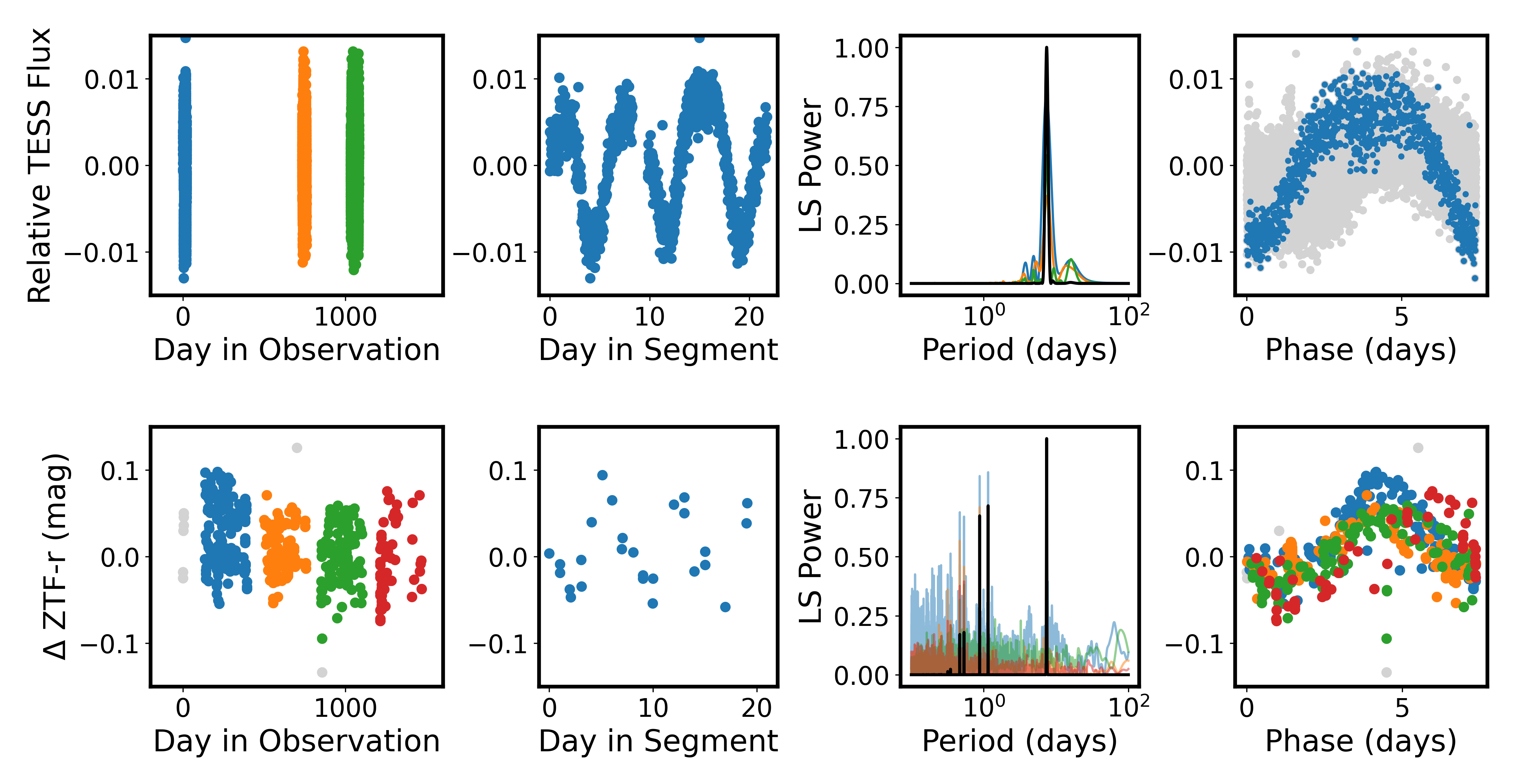
Figure 12: TESS and ZTF light curves and period analysis for the Hyad 2MASS J05512353+1533043 (catalog ) (Gaia DR3 3348035553945613952). Top panels show TESS data and bottom panels show ZTF data. The leftmost panels show all available light curve data (at the time of our analysis), with each survey’s time reference to their first epochs (i.e., both start at zero time). The center-left panels show representative segments of length equal to a single TESS sector ($\approx$27 days). The center-right panels show Lomb–Scargle periodograms for each segment (color-coded for individual sectors for TESS; different seasons for ZTF), and the full data set (black). The rightmost panels present the phase-folded light curves. Despite differences in data quality (total baseline, duration of each sector/season, cadence, precision, angular resolution), the periods precisely agree.

A.2 Two Rapidly Rotating Hyads With Discrepancies Between TESS and ZTF

We present the TESS and ZTF light-curve analyses for two Hyads that have discrepant TESS and ZTF $P_{\mbox{\scriptsize rot}}$ values discussed in Section 5: 2MASS J02594633+3855363 (catalog ) (Gaia DR3 143558461530827264) in Figure 13 and J04461522+1846294 (catalog 2MASS J04461522+1846294) (Gaia DR3 3409867964719693824) in Figure 14.

For the first star, the TESS periodogram shows multiple rapid peaks; the most prominent has a period of 0.3 d. The ZTF periodogram shows some weak peaks in the 0.1–1.0 d range—the highest peak corresponds to 0.2 d and it looks convincingly periodic in the phase-folded light curve. This ZTF period appears to be represented in the TESS periodogram by the second highest peak. Given the high RUWE for this star (=5.0), we conclude it is likely a binary and TESS is detecting periods from both binary components. Perhaps the ZTF periodogram does not show the other significant periods because of the cadence. We adopt the primary TESS period for this star.

For the second star, the TESS periodogram shows two peaks, which are not harmonics. The primary TESS period is 0.24 days, whereas the primary ZTF period is 0.38 d. Although the ZTF periodogram and phase-folded light curves are not convincing on their own, the ZTF period is consistent with the secondary peak in the TESS light curve. For that reason, we consider the two periods detected by TESS to be hosted by the same target (and not caused by an unrelated star blended in the large TESS pixel). As in the first case, this target also boasts an elevated RUWE of 3.4, which indicates that the target is likely a binary. We assign the period for the primary peak in the TESS periodogram as the period for the primary star of the binary, although it is also possible that we have attributed the period to the wrong binary component. However, if that is the case, it will not impact the conclusions of our work: first, the Rossby number for either period places this star in the saturated regime; second, we flag all candidate and confirmed binaries and analyze them separately from the single-star cohort, the latter being the focus of our work.

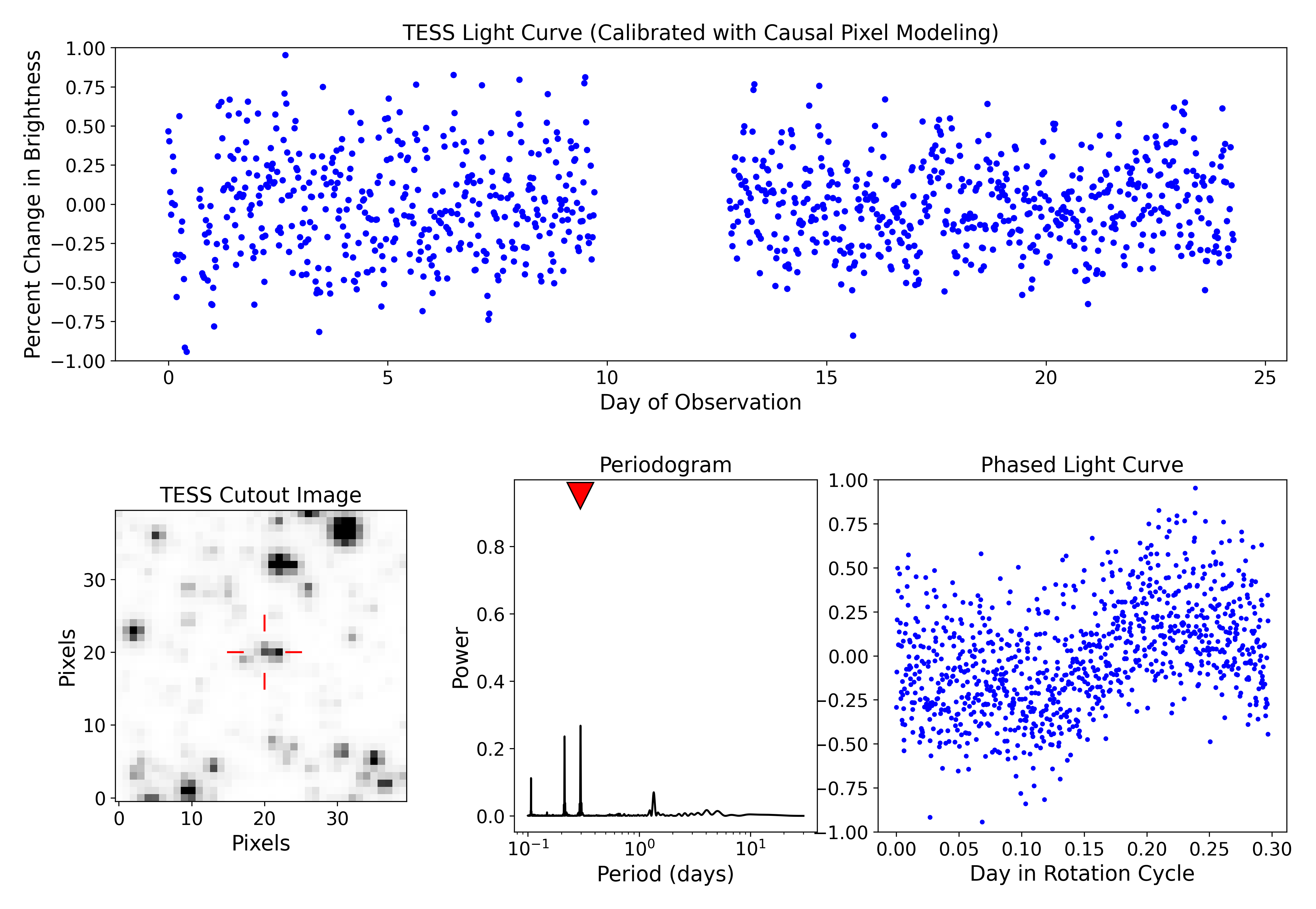
Figure 13: TESS and ZTF light curve analysis for the Hyad 2MASS J02594633+3855363 (catalog ). Top panel: TESS light curve calibrated with Causal Pixel Modeling showing the characteristic gap midway through the 27-day observations. Middle top left: a TESS cutout indicating the position of the star. Middle top center: the Lomb-Scargle periodogram for the TESS light curve shows at least four significant peaks; the one with the highest power is indicated with a red triangle (0.30 d). Middle top right: the phase-folded TESS light curve for the 0.30 d period. Middle bottom: ZTF $r$-band light curve for three seasons. Bottom left: Lomb-Scargle periodogram for ZTF shows a weak peak at 0.21 days. Bottom right: the phase-folded ZTF light curve. We adopt the primary TESS period for this star.

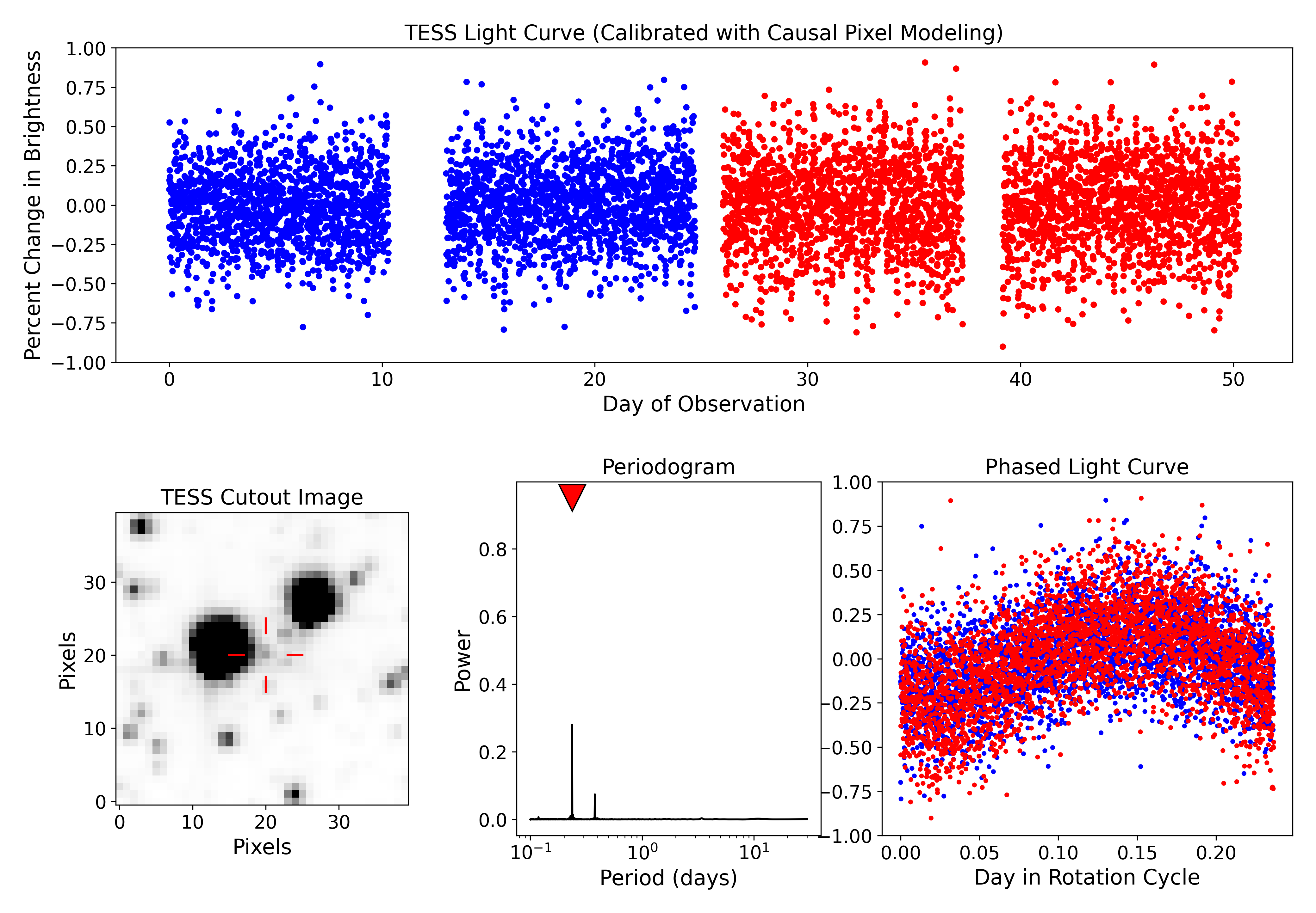
Figure 14: Same as Figure 13 but for the Hyad 2MASS J04461522+1846294 (catalog ). The TESS periodogram shows two significant peaks, the one with the most power being 0.24 d. The ZTF periodogram shows a peak at 0.38 days, but presents an unconvincing phase-folded light curve, so we reject the ZTF period and adopt the primary TESS period for this star.

Appendix B Marginalized Posterior Probability Distributions for the MCMC Analysis of Our $R_{\mathrm{o}}$–$L_{\mathrm{H}\alpha}$/$L_{\mathrm{bol}}$ and $R_{\mathrm{o}}$–$L_{\mathrm{X}}$/$L_{\mathrm{bol}}$ Models

We present the marginalized posterior probability distributions from the MCMC analysis we performed on six different subsamples of Praesepe and Hyades stars: single members of each cluster, binary members of each cluster, single members of both clusters combined, and binary members of both clusters combined (see Section 7.2 and Table 6). The binary samples include candidate and confirmed binaries, which includes stars with RUWE $>$ 1.4. Figure 15 shows an example of the marginalized posterior probability distributions for the combined sample of single members from both clusters for the $R_{\mathrm{o}}$–$L_{\mathrm{H}\alpha}$/$L_{\mathrm{bol}}$ model.

Fig. Set15. Marginalized posterior probability distributions from the MCMC analysis of Our $R_{\mathrm{o}}$–$L_{\mathrm{H}\alpha}$/$L_{\mathrm{bol}}$ and $R_{\mathrm{o}}$–$L_{\mathrm{X}}$/$L_{\mathrm{bol}}$ Models

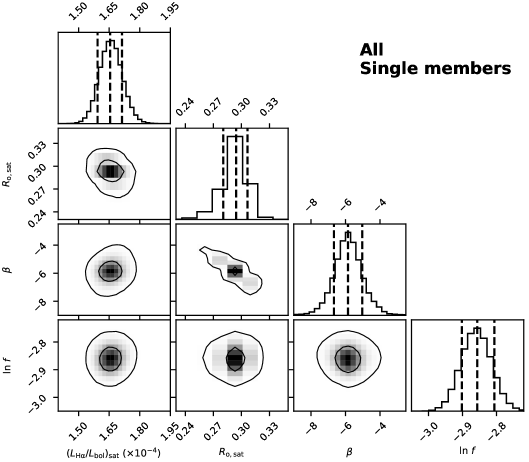
Figure 15: Marginalized posterior probability distributions from the MCMC analysis of our $R_{\mathrm{o}}$–$L_{\mathrm{H}\alpha}$/$L_{\mathrm{bol}}$ model using emcee for single members in both Praesepe and the Hyades. The parameter values of the a posteriori model are the peaks of the one-dimensional distributions; the vertical dashed lines approximate the median and 16^th, 50^th, and 84^th percentiles. The two-dimensional distributions illustrate covariances between parameters; the contour lines approximate the 1$\sigma$ and 2$\sigma$ levels of the distributions. The complete figure set, which includes an image for each of the six subsamples in Table 6 and for both $R_{\mathrm{o}}$–$L_{\mathrm{H}\alpha}$/$L_{\mathrm{bol}}$ and $R_{\mathrm{o}}$–$L_{\mathrm{X}}$/$L_{\mathrm{bol}}$, is available in the online journal.

Appendix C Re-Analysis of the $R_{\mathrm{o}}$–$L_{\mathrm{H}\alpha}$/$L_{\mathrm{bol}}$ Relation Without Applying the Quiescent $\mathrm{H}\alpha$ Absorption Correction

In this Appendix, we include the results we obtained after re-analyzing the $R_{\mathrm{o}}$–$L_{\mathrm{H}\alpha}$/$L_{\mathrm{bol}}$ relation in Section 7.2 without correcting our $\mathrm{H}\alpha$ EW measurements for the quiescent $\mathrm{H}\alpha$ absorption present in these stars (see Section 6.2). This allows us to compare our findings to those of previous studies that did not include this correction, such as Paper II and Núñez et al. (2017).

In Paper II, we found $\beta=-0.73^{+0.16}_{-0.12}$ for the combined sample of Praesepe and Hyades single members. Our new result in this Appendix, $\beta=-1.27^{+0.15}_{-0.17}$, is steeper, but within 2$\sigma$. In that previous study, we also noted a sharp decrease in $L_{\mathrm{H}\alpha}$/$L_{\mathrm{bol}}$ over a small range in $R_{\mathrm{o}}$ for stars with $R_{\mathrm{o}}$ $\gtrsim$ 0.45. Whereas this claim was speculative given the small sample size in Paper II, our current expanded sample allows us to more confidently confirm it.

Our new $R_{\mathrm{o}}$${}_{\mathrm{,sat}}=0.14$$\pm$$0.01$ agrees within 1$\sigma$ with that found in Paper II, $R_{\mathrm{o}}$${}_{\mathrm{,sat}}=0.11^{+0.02}_{-0.03}$. Notably, however, our new ($L_{\mathrm{H}\alpha}$/$L_{\mathrm{bol}}$)_sat = (1.73$\pm$0.06)$\times 10^{-4}$ disagrees with our previous result, ($L_{\mathrm{H}\alpha}$/$L_{\mathrm{bol}}$)_sat = (1.26$\pm$0.04)$\times 10^{-4}$, at the 5$\sigma$ level. This discrepancy is caused by the updated $\chi$ values that we used to calculate $L_{\mathrm{H}\alpha}$/$L_{\mathrm{bol}}$ in this work. As shown in Figure 5, our updated $\chi$ values are $\approx$1.3$\times$ larger than those used in Paper II.

In Núñez et al. (2017), we found $\beta=-0.51$$\pm$$0.02$ for a sample of single cluster members in the $\approx$500-Myr-old open cluster M37. Our $\beta$ in this Appendix for the combined sample of Praesepe and Hyades disagrees with the M37 result at the 5$\sigma$ level. We point out two issues that may be driving this large difference. First, the sample of $\mathrm{H}\alpha$ EW measurements in the M37 study was partly contaminated by $\mathrm{H}\alpha$ emission from a foreground nebula. In that work, an attempt was made to mitigate the impact of the $\mathrm{H}\alpha$ nebular emission by excluding stars for which [N ii] emission $\leq-3$ Å. However, this still left stars with mildly contaminated $\mathrm{H}\alpha$ EW values in the sample, leading to artificially higher $L_{\mathrm{H}\alpha}$/$L_{\mathrm{bol}}$ values for those stars and potentially a shallower value for the best-fit $\beta$.

Second, the largest $R_{\mathrm{o}}$ value for a M37 member in that study is $\approx$0.4, while our study shows the sharpest $L_{\mathrm{H}\alpha}$/$L_{\mathrm{bol}}$ decline at $R_{\mathrm{o}}$ $\gtrsim$ 0.4. In addition, most of the M37 stars with the lowest $L_{\mathrm{H}\alpha}$/$L_{\mathrm{bol}}$ and largest $R_{\mathrm{o}}$ values in the unsaturated regime have $L_{\mathrm{H}\alpha}$/$L_{\mathrm{bol}}$ uncertainties larger than those in our sample. The MCMC algorithm that calculates $\beta$ incorporates the uncertainty associated with each measurement by assigning weights to individual data points. Therefore, these larger $L_{\mathrm{H}\alpha}$/$L_{\mathrm{bol}}$ uncertainties in the M37 sample probably resulted in a shallower $\beta$.

Our new $R_{\mathrm{o}}$_,sat for the combined sample of Praesepe and Hyades stars is larger than the M37 $R_{\mathrm{o}}$${}_{\mathrm{,sat}}=0.03\pm 0.01$ by a factor of almost 5. Also, our new ($L_{\mathrm{H}\alpha}$/$L_{\mathrm{bol}}$)_sat disagrees with the M37 ($L_{\mathrm{H}\alpha}$/$L_{\mathrm{bol}}$)_sat = (1.27$\pm$0.01)$\times 10^{-4}$ at the $>$5$\sigma$ level. Although the latter discrepancy is mostly explained by the aforementioned differences in $\chi$ values between the two studies, we found no evident explanation for the discrepancy in $R_{\mathrm{o}}$_,sat. Outdated M37 stellar parameters, including cluster membership, may be partly driving the large differences in the characterization of the $R_{\mathrm{o}}$–$L_{\mathrm{H}\alpha}$/$L_{\mathrm{bol}}$ relation between our study and that of M37.

Figure 16: Same as Figure 7, but with $L_{\mathrm{H}\alpha}$/$L_{\mathrm{bol}}$ calculated using our measured EW values instead of relative EW values from Section 6.2. The latter account for the $\mathrm{H}\alpha$ quiescent photospheric absorption present in these stars.

References

- Alexander & Preibisch (2012) Alexander, F., & Preibisch, T. 2012, A&A, 539, A64, doi: 10.1051/0004-6361/201118100
- Allen & Strom (1995) Allen, L. E., & Strom, K. M. 1995, AJ, 109, 1379, doi: 10.1086/117370
- Argiroffi et al. (2016) Argiroffi, C., Caramazza, M., Micela, G., et al. 2016, A&A, 589, A113, doi: 10.1051/0004-6361/201526539
- Astropy Collaboration et al. (2022) Astropy Collaboration, Price-Whelan, A. M., Lim, P. L., et al. 2022, ApJ, 935, 167, doi: 10.3847/1538-4357/ac7c74
- Brasseur et al. (2019) Brasseur, C. E., Phillip, C., Fleming, S. W., Mullally, S. E., & White, R. L. 2019, Astrocut: Tools for creating cutouts of TESS images, Astrophysics Source Code Library, record ascl:1905.007. http://ascl.net/1905.007
- Brown et al. (1991) Brown, S. F., Donati, J. F., Rees, D. E., & Semel, M. 1991, A&A, 250, 463
- Campbell et al. (1983) Campbell, B., Mein, N., Mein, P., et al. 1983, A&A, 123, 89
- Cook et al. (2014) Cook, B. A., Williams, P. K. G., & Berger, E. 2014, ApJ, 785, 10, doi: 10.1088/0004-637X/785/1/10
- Cram (1982) Cram, L. E. 1982, ApJ, 253, 768, doi: 10.1086/159679
- Cummings et al. (2018) Cummings, J. D., Kalirai, J. S., Tremblay, P. E., Ramirez-Ruiz, E., & Choi, J. 2018, ApJ, 866, 21, doi: 10.3847/1538-4357/aadfd6
- Curtis et al. (2021) Curtis, J. L., Popinchalk, M., Douglas, S. T., et al. 2021, tess_check, https://github.com/SPOT-FFI/tess_check, GitHub
- Curtis et al. (2020) Curtis, J. L., Agüeros, M. A., Matt, S. P., et al. 2020, ApJ, 904, 140, doi: 10.3847/1538-4357/abbf58
- Deacon & Kraus (2020) Deacon, N. R., & Kraus, A. L. 2020, MNRAS, 496, 5176, doi: 10.1093/mnras/staa1877
- Douglas et al. (2016) Douglas, S. T., Agüeros, M. A., Covey, K. R., et al. 2016, ApJ, 822, 47, doi: 10.3847/0004-637X/822/1/47
- Douglas et al. (2017) Douglas, S. T., Agüeros, M. A., Covey, K. R., & Kraus, A. 2017, ApJ, 842, 83, doi: 10.3847/1538-4357/aa6e52
- Douglas et al. (2019) Douglas, S. T., Curtis, J. L., Agüeros, M. A., et al. 2019, ApJ, 879, 100, doi: 10.3847/1538-4357/ab2468
- Douglas et al. (2014) Douglas, S. T., Agüeros, M. A., Covey, K. R., et al. 2014, ApJ, 795, 161, doi: 10.1088/0004-637X/795/2/161
- Fabricant et al. (2005) Fabricant, D., Fata, R., Roll, J., et al. 2005, PASP, 117, 1411, doi: 10.1086/497385
- Fan (2021) Fan, Y. 2021, Living Reviews in Solar Physics, 18, 5, doi: 10.1007/s41116-021-00031-2
- Foreman-Mackey et al. (2013) Foreman-Mackey, D., Hogg, D. W., Lang, D., & Goodman, J. 2013, PASP, 125, 306, doi: 10.1086/670067
- Fruscione et al. (2006) Fruscione, A., McDowell, J. C., Allen, G. E., et al. 2006, in Proc. SPIE, Vol. 6270, Proc. SPIE, 1, doi: 10.1117/12.671760
- Gaia Collaboration et al. (2018a) Gaia Collaboration, Brown, A. G. A., Vallenari, A., et al. 2018a, A&A, 616, A1, doi: 10.1051/0004-6361/201833051
- Gaia Collaboration et al. (2018b) Gaia Collaboration, Babusiaux, C., van Leeuwen, F., et al. 2018b, A&A, 616, A10, doi: 10.1051/0004-6361/201832843
- Gaia Collaboration et al. (2022) Gaia Collaboration, Vallenari, A., Brown, A. G. A., et al. 2022, arXiv e-prints, arXiv:2208.00211, doi: 10.48550/arXiv.2208.00211
- Ginsburg & Mirocha (2011) Ginsburg, A., & Mirocha, J. 2011, PySpecKit: Python Spectroscopic Toolkit, Astrophysics Source Code Library. http://ascl.net/1109.001
- Güdel (2004) Güdel, M. 2004, A&A Rev., 12, 71, doi: 10.1007/s00159-004-0023-2
- Harris et al. (2020) Harris, C. R., Millman, K. J., van der Walt, S. J., et al. 2020, Nature, 585, 357, doi: 10.1038/s41586-020-2649-2
- Hattori et al. (2022) Hattori, S., Foreman-Mackey, D., Hogg, D. W., et al. 2022, AJ, 163, 284, doi: 10.3847/1538-3881/ac625a
- He et al. (2019) He, L., Wang, S., Liu, J., et al. 2019, ApJ, 871, 193, doi: 10.3847/1538-4357/aaf8b7
- Hodgkin et al. (1995) Hodgkin, S. T., Jameson, R. F., & Steele, I. A. 1995, MNRAS, 274, 869
- Howell et al. (2014) Howell, S. B., Sobeck, C., Haas, M., et al. 2014, PASP, 126, 398, doi: 10.1086/676406
- Hunter (2007) Hunter, J. D. 2007, Computing in Science & Engineering, 9, 90, doi: 10.1109/MCSE.2007.55
- Husser et al. (2013) Husser, T.-O., Wende-von Berg, S., Dreizler, S., et al. 2013, A&A, 553, A6, doi: 10.1051/0004-6361/201219058
- IRSA (2022) IRSA. 2022, Zwicky Transient Facility Image Service, IPAC, doi: 10.26131/IRSA539
- Jackson & Jeffries (2010) Jackson, R. J., & Jeffries, R. D. 2010, MNRAS, 407, 465, doi: 10.1111/j.1365-2966.2010.16917.x
- James et al. (2000) James, D. J., Jardine, M. M., Jeffries, R. D., et al. 2000, MNRAS, 318, 1217, doi: 10.1046/j.1365-8711.2000.03838.x
- Jardine (2004) Jardine, M. 2004, A&A, 414, L5, doi: 10.1051/0004-6361:20031723
- Jardine & Unruh (1999) Jardine, M., & Unruh, Y. C. 1999, A&A, 346, 883
- Jeffries et al. (2011) Jeffries, R. D., Jackson, R. J., Briggs, K. R., Evans, P. A., & Pye, J. P. 2011, MNRAS, 411, 2099, doi: 10.1111/j.1365-2966.2010.17848.x
- Kafka & Honeycutt (2004) Kafka, S., & Honeycutt, R. K. 2004, Astronomische Nachrichten, 325, 413, doi: 10.1002/asna.200310242
- Kafka & Honeycutt (2006) —. 2006, AJ, 132, 1517, doi: 10.1086/506561
- Kervella et al. (2022) Kervella, P., Arenou, F., & Thévenin, F. 2022, A&A, 657, A7, doi: 10.1051/0004-6361/202142146
- Kraus & Hillenbrand (2007) Kraus, A. L., & Hillenbrand, L. A. 2007, AJ, 134, 2340, doi: 10.1086/522831
- Kraus et al. (2016) Kraus, A. L., Ireland, M. J., Huber, D., Mann, A. W., & Dupuy, T. J. 2016, AJ, 152, 8, doi: 10.3847/0004-6256/152/1/8
- Law et al. (2010) Law, N. M., Dekany, R. G., Rahmer, G., et al. 2010, in Society of Photo-Optical Instrumentation Engineers (SPIE) Conference Series, Vol. 7735, Society of Photo-Optical Instrumentation Engineers (SPIE) Conference Series, doi: 10.1117/12.857400
- Linsky et al. (1982) Linsky, J. L., Bornmann, P. L., Carpenter, K. G., et al. 1982, ApJ, 260, 670, doi: 10.1086/160288
- Magaudda et al. (2020) Magaudda, E., Stelzer, B., Covey, K. R., et al. 2020, A&A, 638, A20, doi: 10.1051/0004-6361/201937408
- Marsden et al. (2009) Marsden, S. C., Carter, B. D., & Donati, J.-F. 2009, MNRAS, 399, 888, doi: 10.1111/j.1365-2966.2009.15319.x
- Masci et al. (2018) Masci, F. J., Laher, R. R., Rusholme, B., et al. 2018, Publications of the Astronomical Society of the Pacific, 131, 018003, doi: 10.1088/1538-3873/aae8ac
- Masci et al. (2019) Masci, F. J., Laher, R. R., Rusholme, B., et al. 2019, PASP, 131, 018003, doi: 10.1088/1538-3873/aae8ac
- McDivitt et al. (2022) McDivitt, J., Douglas, S. T., Curtis, J. L., Popinchalk, M., & Núñez, A. 2022, Research Notes of the American Astronomical Society, 6, 116, doi: 10.3847/2515-5172/ac7793
- Meibom et al. (2007) Meibom, S., Mathieu, R. D., & Stassun, K. G. 2007, ApJ, 665, L155, doi: 10.1086/521437
- Messina et al. (2017) Messina, S., Lanzafame, A. C., Malo, L., et al. 2017, A&A, 607, A3, doi: 10.1051/0004-6361/201730444
- Miesch (2005) Miesch, M. S. 2005, Living Reviews in Solar Physics, 2, 1, doi: 10.12942/lrsp-2005-1
- Mullan (1976) Mullan, D. J. 1976, ApJ, 207, 289, doi: 10.1086/154492
- Nelson et al. (2013) Nelson, N. J., Brown, B. P., Brun, A. S., Miesch, M. S., & Toomre, J. 2013, ApJ, 762, 73, doi: 10.1088/0004-637X/762/2/73
- Newton et al. (2017) Newton, E. R., Irwin, J., Charbonneau, D., et al. 2017, ApJ, 834, 85, doi: 10.3847/1538-4357/834/1/85
- Noyes et al. (1984) Noyes, R. W., Weiss, N. O., & Vaughan, A. H. 1984, ApJ, 287, 769, doi: 10.1086/162735
- Núñez et al. (2017) Núñez, A., Agüeros, M. A., Covey, K. R., & López-Morales, M. 2017, ApJ, 834, 176, doi: 10.3847/1538-4357/834/2/176
- Núñez et al. (2022a) Núñez, A., Douglas, S. T., Alam, M., & Stan, D. 2022a, PHEW: PytHon Equivalent Widths, v2.0, Zenodo, doi: 10.5281/zenodo.6422571
- Núñez et al. (2015) Núñez, A., Agüeros, M. A., Covey, K. R., et al. 2015, ApJ, 809, 161, doi: 10.1088/0004-637X/809/2/161
- Núñez et al. (2022b) —. 2022b, ApJ, 931, 45, doi: 10.3847/1538-4357/ac6517
- Ochsenbein et al. (2000) Ochsenbein, F., Bauer, P., & Marcout, J. 2000, A&AS, 143, 23
- Ossendrijver (2003) Ossendrijver, M. 2003, A&A Rev., 11, 287, doi: 10.1007/s00159-003-0019-3
- Parker (1993) Parker, E. N. 1993, ApJ, 408, 707, doi: 10.1086/172631
- Pecaut & Mamajek (2013) Pecaut, M. J., & Mamajek, E. E. 2013, ApJS, 208, 9, doi: 10.1088/0067-0049/208/1/9
- Pevtsov et al. (2003) Pevtsov, A. A., et al. 2003, ApJ, 598, 1387, doi: 10.1086/378944
- Pizzolato et al. (2003) Pizzolato, N., Maggio, A., Micela, G., Sciortino, S., & Ventura, P. 2003, A&A, 397, 147, doi: 10.1051/0004-6361:20021560
- Preibisch & Feigelson (2005) Preibisch, T., & Feigelson, E. D. 2005, ApJS, 160, 390, doi: 10.1086/432094
- Press & Rybicki (1989) Press, W. H., & Rybicki, G. B. 1989, Astrophysical Journal, 338, 277, doi: 10.1086/167197
- Prochaska et al. (2020) Prochaska, J. X., Hennawi, J. F., Westfall, K. B., et al. 2020, Journal of Open Source Software, 5, 2308, doi: 10.21105/joss.02308
- Prochaska et al. (2020) Prochaska, J. X., Hennawi, J., Cooke, R., et al. 2020, pypeit/PypeIt: Release 1.0.0, v1.0.0, Zenodo, Zenodo, doi: 10.5281/zenodo.3743493
- Prosser et al. (1996) Prosser, C. F., Randich, S., Stauffer, J. R., Schmitt, J. H. M. M., & Simon, T. 1996, AJ, 112, 1570, doi: 10.1086/118124
- Rampalli et al. (2021) Rampalli, R., Agüeros, M. A., Curtis, J. L., et al. 2021, ApJ, 921, 167, doi: 10.3847/1538-4357/ac0c1e
- Randich (1998) Randich, S. 1998, in Astronomical Society of the Pacific Conference Series, Vol. 154, Cool Stars, Stellar Systems, and the Sun, ed. R. A. Donahue & J. A. Bookbinder, 501. https://arxiv.org/abs/astro-ph/9709177
- Randich (2000) Randich, S. 2000, in Astronomical Society of the Pacific Conference Series, Vol. 198, Stellar Clusters and Associations: Convection, Rotation, and Dynamos, ed. R. Pallavicini, G. Micela, & S. Sciortino, 401
- Randich et al. (1996) Randich, S., Schmitt, J. H. M. M., Prosser, C. F., & Stauffer, J. R. 1996, A&A, 305, 785
- Rebull et al. (2006) Rebull, L. M., Stauffer, J. R., Megeath, S. T., Hora, J. L., & Hartmann, L. 2006, ApJ, 646, 297, doi: 10.1086/504865
- Reid & Hawley (2005) Reid, I. N., & Hawley, S. L. 2005, New light on dark stars : red dwarfs, low-mass stars, brown dwarfs (Praxis Publishing Ltd), doi: 10.1007/3-540-27610-6
- Reiners & Basri (2007) Reiners, A., & Basri, G. 2007, ApJ, 656, 1121, doi: 10.1086/510304
- Reiners & Basri (2010) —. 2010, ApJ, 710, 924, doi: 10.1088/0004-637X/710/2/924
- Reiners & Mohanty (2012) Reiners, A., & Mohanty, S. 2012, ApJ, 746, 43, doi: 10.1088/0004-637X/746/1/43
- Richey-Yowell et al. (2019) Richey-Yowell, T., Shkolnik, E. L., Schneider, A. C., et al. 2019, ApJ, 872, 17, doi: 10.3847/1538-4357/aafa74
- Ricker et al. (2015) Ricker, G. R., Winn, J. N., Vanderspek, R., et al. 2015, J. Astron. Telesc. Instrum. Syst., 1, 014003, doi: 10.1117/1.JATIS.1.1.014003
- Schrijver et al. (1989) Schrijver, C. J., Cote, J., Zwaan, C., & Saar, S. H. 1989, ApJ, 337, 964, doi: 10.1086/167168
- Science Software Branch at STScI (2012) Science Software Branch at STScI. 2012, PyRAF: Python alternative for IRAF, Astrophysics Source Code Library, record ascl:1207.011. http://ascl.net/1207.011
- See et al. (2019) See, V., Matt, S. P., Folsom, C. P., et al. 2019, ApJ, 876, 118, doi: 10.3847/1538-4357/ab1096
- Skrutskie et al. (2006) Skrutskie, M. F., Cutri, R. M., Stiening, R., et al. 2006, AJ, 131, 1163, doi: 10.1086/498708
- Solanki et al. (1997) Solanki, S. K., Motamen, S., & Keppens, R. 1997, A&A, 324, 943
- Stauffer et al. (1997a) Stauffer, J. R., Balachandran, S. C., Krishnamurthi, A., et al. 1997a, ApJ, 475, 604, doi: 10.1086/303567
- Stauffer et al. (1994) Stauffer, J. R., Caillault, J.-P., Gagne, M., Prosser, C. F., & Hartmann, L. W. 1994, ApJS, 91, 625, doi: 10.1086/191951
- Stauffer & Hartmann (1986) Stauffer, J. R., & Hartmann, L. W. 1986, ApJS, 61, 531, doi: 10.1086/191123
- Stauffer et al. (1997b) Stauffer, J. R., Hartmann, L. W., Prosser, C. F., et al. 1997b, ApJ, 479, 776, doi: 10.1086/303930
- Stȩpień et al. (2001) Stȩpień, K., Schmitt, J. H. M. M., & Voges, W. 2001, A&A, 370, 157, doi: 10.1051/0004-6361:20010197
- Stelzer et al. (2016) Stelzer, B., Damasso, M., Scholz, A., & Matt, S. P. 2016, MNRAS, 463, 1844, doi: 10.1093/mnras/stw1936
- Stelzer et al. (2013) Stelzer, B., Marino, A., Micela, G., López-Santiago, J., & Liefke, C. 2013, MNRAS, 431, 2063, doi: 10.1093/mnras/stt225
- Stelzer & Neuhäuser (2001) Stelzer, B., & Neuhäuser, R. 2001, A&A, 377, 538, doi: 10.1051/0004-6361:20011093
- Thiemann et al. (2020) Thiemann, H. B., Norton, A. J., & Kolb, U. C. 2020, PASA, 37, e042, doi: 10.1017/pasa.2020.33
- Tody (1986) Tody, D. 1986, in Society of Photo-Optical Instrumentation Engineers (SPIE) Conference Series, Vol. 627, Instrumentation in astronomy VI, ed. D. L. Crawford, 733, doi: 10.1117/12.968154
- Vaiana et al. (1981) Vaiana, G. S., Cassinelli, J. P., Fabbiano, G., et al. 1981, ApJ, 245, 163, doi: 10.1086/158797
- van Leeuwen (2009) van Leeuwen, F. 2009, A&A, 497, 209, doi: 10.1051/0004-6361/200811382
- Vernazza et al. (1981) Vernazza, J. E., Avrett, E. H., & Loeser, R. 1981, ApJS, 45, 635, doi: 10.1086/190731
- Vilhu (1984) Vilhu, O. 1984, A&A, 133, 117
- Virtanen et al. (2020) Virtanen, P., Gommers, R., Oliphant, T. E., et al. 2020, Nature Methods, 17, 261, doi: 10.1038/s41592-019-0686-2
- Wang et al. (2016) Wang, D., Hogg, D. W., Foreman-Mackey, D., & Schölkopf, B. 2016, PASP, 128, 094503, doi: 10.1088/1538-3873/128/967/094503
- Webb et al. (2020) Webb, N. A., Coriat, M., Traulsen, I., et al. 2020, A&A, 641, A136, doi: 10.1051/0004-6361/201937353
- Wright et al. (2011) Wright, N. J., Drake, J. J., Mamajek, E. E., & Henry, G. W. 2011, ApJ, 743, 48, doi: 10.1088/0004-637X/743/1/48
- Wright et al. (2018) Wright, N. J., Newton, E. R., Williams, P. K. G., Drake, J. J., & Yadav, R. K. 2018, MNRAS, 479, 2351, doi: 10.1093/mnras/sty1670
- York et al. (2000) York, D. G., Adelman, J., Anderson, John E., J., et al. 2000, AJ, 120, 1579, doi: 10.1086/301513
- Ziegler et al. (2020) Ziegler, C., Tokovinin, A., Briceño, C., et al. 2020, AJ, 159, 19, doi: 10.3847/1538-3881/ab55e9
- Ziegler et al. (2018) Ziegler, C., Law, N. M., Baranec, C., et al. 2018, AJ, 156, 259, doi: 10.3847/1538-3881/aad80a