Splitwise: Efficient Generative LLM Inference Using Phase Splitting

Abstract

Recent innovations in generative large language models (LLMs) have made their applications and use-cases ubiquitous. This has led to large-scale deployments of these models, using complex, expensive, and power-hungry AI accelerators, most commonly GPUs. These developments make LLM inference efficiency an important challenge. Based on our extensive characterization, we find that there are two main phases during an LLM inference request: a compute-intensive prompt computation, and a memory-intensive token generation, each with distinct latency, throughput, memory, and power characteristics. Despite state-of-the-art batching and scheduling, the token generation phase underutilizes compute resources. Specifically, unlike compute-intensive prompt computation phases, token generation phases do not require the compute capability of the latest GPUs, and can be run with lower power and cost.

With Splitwise, we propose splitting the two phases of a LLM inference request on to separate machines. This allows us to use hardware that is well-suited for each phase, and provision resources independently per phase. However, splitting an inference request across machines requires state transfer from the machine running prompt computation over to the machine generating tokens. We implement and optimize this state transfer using the fast back-plane interconnects available in today’s GPU clusters.

We use the Splitwise technique to design LLM inference clusters using the same or different types of machines for the prompt computation and token generation phases. Our clusters are optimized for three key objectives: throughput, cost, and power. In particular, we show that we can achieve $1.4\times$ higher throughput at 20% lower cost than current designs. Alternatively, we can achieve $2.35\times$ more throughput with the same cost and power budgets.

I Introduction

Generative Large Language Models (LLMs) have seen a lot of progress in response quality and accuracy recently [15, 43]. This has led to a wide adoption of LLMs for various use-cases [4, 17]. Most modern LLMs are based on transformers [46, 45], and share very similar characteristics [36]. Most of these models are large, and run on expensive and power-hungry GPUs [14]. The sudden large-scale deployment of LLMs has led to a world-wide GPUs capacity crunch [12].

While it is important to train these LLMs efficiently, the bulk of the datacenters and machines are being used for inference instead. The reason is the vast number of use-cases that leverage LLMs. Furthermore, the cost of training these models is very high and requires dedicated super-computers [35, 31]. A large number of inferences is the way to amortize/offset the high training costs. LLM inference jobs, although orders of magnitude smaller than training, are still expensive given the compute involved. The model size (the number of parameters in transformers models) has grown steadily, from the early BERT models [24] having 340 million parameters to GPT3 [22] with 175 billion parameters, and GPT4 rumored to have even more.

	A100	H100	Ratio
TFLOPs	19.5	66.9	3.43$\times$
HBM capacity	80GB	80GB	1.00$\times$
HBM bandwidth	2039GBps	3352GBps	1.64$\times$
Power	400W	700W	1.75$\times$
NVLink	50 Gbps	100Gbps	2.00$\times$
Infiniband	200GBps	400GBps	2.00$\times$
Cost per machine [3]	$17.6/hr	$38/hr	2.16$\times$

TABLE I: NVIDIA A100 vs. H100 relevant specifications.

Generative LLM inference in all the current models for a single request consists of several forward passes of the model, as the output tokens are generated one by one. This inherently has two contrasting phases of computation. First, the prompt computation phase where all the tokens in the input prompt run through the forward pass of the model in parallel, to generate the first output token. This phase tends to be computationally intensive and requires the high FLOPs (floating point operations per second) of the latest GPUs today. Second, the token generation phase which tends to be more serialized in nature, as each token is generated based on the forward pass of the last token and all the cached context from previous tokens in the sequence. Given the lack of parallelism in this computation, this phase tends to be more memory bandwidth and capacity bound, despite state-of-the-art batching. Running both phases on the same machine leads to inconsistent end-to-end latency. Due to these challenges, services need to over-provision these expensive GPUs to meet tight inference service level objectives (SLOs). On the other hand, cloud service providers (CSPs) are building many new datacenters for GPU expansions, and running into a power wall [16].

Meanwhile, the industry continues to release more and more computationally able GPUs, each much more power-hungry and expensive than the previous one. However, as shown in Table I, the high-bandwidth memory (HBM) capacity and bandwidth on these GPUs has not scaled at the same rate recently. The latest NVIDIA H100 GPUs have $3.43\times$ more compute and $1.75\times$ more power as compared to their predecessor A100 GPUs. But the memory bandwidth increase was limited to $1.6\times$, with no increase in memory capacity.

Our work. Given the clear phases in the computation of an inference request for generative LLMs, we propose separating the prompt computation and the token generation phases onto separate machines. This increases hardware utilization and therefore the overall efficiency of the system. It also enables using different, better-provisioned hardware for each phase To realize such a setup, the cached context from the prompt computation will have to be communicated over from the prompt machine to the token machine with low latency. We implement these transfers in an optimized way using available bandwidths, which allows us to increase efficiency without any perceived performance loss.

With Splitwise, we design clusters optimized for cost, throughput, and power, based on production traces of LLM inference requests. Given the aforementioned diverging memory and compute expansions over the generations of GPUs, we also evaluate different GPUs and power caps for the different inference phases. This allows us to target better performance per dollar (Perf/$) for users, and better performance per watt (Perf/W) for CSPs. Additionally, users are also to target older GPUs, which are likely more readily available to them.

We show that with Splitwise-based LLM inference clusters, we can achieve 1.4$\times$ higher throughput at 20% lower cost. Alternatively, we can achieve 2.35$\times$ more throughput with the same cost and power budgets.

Summary. In this paper, we make the following contributions:

1. An extensive characterization of the differences in the execution and utilization patterns of the prompt and token generation phases using production traces on the two latest flagship GPUs from NVIDIA: A100 and H100.

2. Splitwise, our technique for optimized utilization of available hardware by separating the prompt computation and token generation phases onto separate machines.

3. Designing homogeneous and heterogeneous clusters with Splitwise to optimize cost, throughput, and power.

4. And finally an evaluation of the systems designed with Splitwise, using production traces.

II Background

II-A Large Language Models

Modern LLMs are based on transformers. Transformer models use attention [45] and multi-layer-perceptron layers to understand the inputs and generate an output, respectively. Transformer-based LLMs can consist of encoder-only [24, 29], decoder-only [40, 41, 43] or encoder-decoder [42] models. Generative LLMs, the focus of this paper, are usually either decoder-only or encoder-decoder models.

II-B Generative LLM inference phases

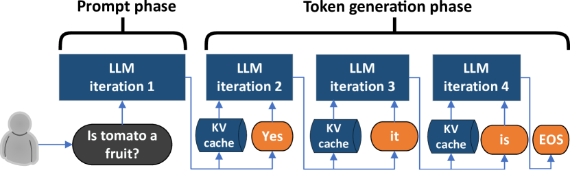
Figure 1 shows an example of generative LLM inference. Once the prompt query is received, all the input tokens are computed in parallel, in a single iteration to generate the first token. We term this as the prompt processing phase. The context generated from the attention layers during the prompt computation is saved in the key-value (KV) cache, since it is needed for all the future token generation iterations. After the first token is generated, the following tokens only use the last generated token and the KV-cache as inputs to the forward pass of the model. This makes the subsequent token generation more memory bandwidth and capacity intensive than the computationally heavy prompt phase.

In this paper, we separate the prompt and token phases of a generative LLM inference onto separate machines.

Figure 1: An LLM inference example.

II-C Performance metrics for LLMs

Prior work has proposed three main metrics for LLM inference: end-to-end (E2E) latency, time to first token (TTFT), and throughput. We add another latency metric: time between tokens (TBT), to track the online streaming throughput of the tokens as they are generated serially. Table II summarizes the key performance metrics that we consider in this work.

Metric	Importance to user
End-to-end (E2E) latency	Total query time that the user sees
Time to first token (TTFT)	How quickly user sees initial response
Time between tokens (TBT)	Average token streaming latency
Throughput	Requests per second

TABLE II: Performance metrics for LLMs.

Generative LLMs may be used for a variety of tasks with different kinds of SLOs. For batch tasks (e.g., summarization), TTFT or TBT latency metrics are less important than throughput. On the other hand, for latency-sensitive tasks (e.g., conversational APIs), TTFT and TBT are the more important metrics with tighter SLOs.

Figure 2: Batching mechanisms and their latency impact on the prompt and token phases.

II-D Batching of requests

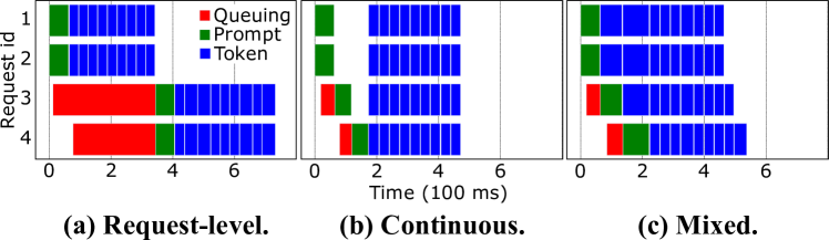
Requests reaching an inference machine can be batched for higher throughput. Several previous works have explored batching [48, 19]. Figure 2 shows the timelines for inference with three common batching mechanisms. The default mechanism only batches at the request-level (Figure 2(a)). In this case, ready requests are batched together, but all the forward passes for these requests are completed before any other requests are run. Since requests can have long token generation phases, this can lead to long wait times for requests arriving in between, causing high TTFT and high E2E latencies. An optimization is continuous batching [48] (Figure 2(b)). In this case, the scheduling decisions are made before each forward pass. However, any given batch comprises either purely of prompt phase, or only token phase. Prompt phase is considered more important since it impacts the prompt phase (i.e., TTFT). Hence, a waiting prompt can preempt a token phase. Although this leads to shorter TTFT, it can increase the tail for TBT, and therefore E2E by a lot. Finally, there is mixed batching (Figure 2(c)) [19]. With this batching, the scheduling decisions are made at each forward pass, and the prompt and token phases can run together. This reduces the impact on TBT, but does not eliminate it, since token phases scheduled with prompt phases will experience a longer runtime. In the rest of the paper, we use mixed batching unless stated otherwise.

II-E Model parallelism

Given the increasing model sizes, model parallelism is no longer just applicable to training, but also inference. Model parallelism can be used to divide a model onto multiple GPUs, and even multiple machines. There are two types of model parallelism used in inference: pipeline and tensor. Pipeline parallelism (PP) divides the layers of the model among the GPUs, while keeping all the operators and tensors within a layer on the same GPU. Tensor parallelism (TP) on the other hand, divides the tensor across the GPUs, while replicating all the layers on each GPU. Pipeline parallelism requires lower communication across the participating GPUs, while tensor parallelism requires high bandwidth communication for each layer. In general, tensor parallelism is known to be better performing for GPUs within the same machine, connected with very high bandwidth interconnect. In the rest of the paper, we use tensor parallelism across 8 GPUs for the best latency.

II-F GPU clusters and interconnects

With the rise of LLM use-cases in the past years, several CSPs have expanded the GPU-based offerings, leading to large GPU cluster deployments [31, 32, 3]. Each machine in these AI clusters generally comprises 8 flagship NVIDIA GPUs (A100 or H100). Each GPUs is connected to all the other GPUs in the cluster with high bandwidth interconnects like Mellanox InfiniBand [11, 8], forming a high bandwidth data plane. The InfiniBand bandwidth offered in the cloud today ranges from 25GBps per GPU to 50GBps per GPU [8, 5]. The default optimized communication library across GPUs over NVLink or InfiniBand is NCCL [13].

III Characterization

In this section, we explore the performance and utilization characteristics of LLM inference, and draw key insights to guide the design of Splitwise.

Production traces. We use production traces taken from a large cloud provider, Azure. The traces are 20 minutes long and include the arrival time, input size (number of prompt tokens), and output size (number of output tokens). We use traces representing the most common scenarios in LLM inference today: coding and conversation. Since LLM output quality has no impact on the issues we explore in this work, for each request in the trace, we use randomized text inputs that match the number of input tokens, and force the LLM to generate the right number of tokens as per the trace. For this characterization, we do not reuse any KV-cache between requests to emulate a cloud service with security guarantees. We do account for KV-cache transfers in the evaluation.

Models. Table III shows the models that we evaluate. Both BLOOM [41] and Llama2 [43] are open source models, considered to be state of the art in the generative LLM community. Both models are decoder-only transformer-based models. We use the version of each model with the most parameters, since these versions are the most representative of production-class accuracy. Unless stated otherwise, we run BLOOM-176B and Llama2-70B on vLLM [27] on a machine with 8 H100 [14] GPUs.

Model	#Layers	Hidden size	#Heads
Llama2-70B	80	8192	32
BLOOM-176B	70	14336	112

TABLE III: Models we evaluate and their parameters.

III-A Number of prompt and generated tokens

To better understand these traces, we look at the distribution in the number of prompt input and generated output tokens. Figure 3(a) shows the distribution of number of prompt tokens. Since the coding LLM inference service is generally used to generate completions, as the user is writing code, the input prompt to this inference can include large chunks of the code written so far. This shows in the distribution, as the median prompt size is 1500 tokens. On the other hand, the conversation service has a wider range of input prompt tokens, as it depends on the user. The median number of prompt tokens for this trace is 1020 tokens.

(a)

(b)

Figure 3: Distribution for prompt and generated tokens.

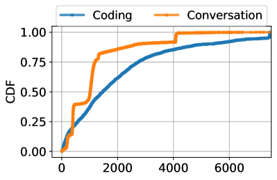
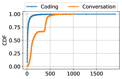
Figure 3(b) shows the distribution in the number of generated tokens. Since the common case for the coding service would only need to generate the next few words in the program as the user is typing, the median number of output token is 13 tokens. On the other hand, the conversation service has an almost bimodal distribution, with a median of 129 tokens generated.

Insight I: Different inference services may have widely different prompt and token distributions.

Figure 4: Cumulative distribution of time spent with various batched tokens.

(a)

(b)

(c)

Figure 5: Latencies for BLOOM-176B and Llama2-70B on DGX-H100.

III-B Batch utilization

To understand how much these requests can be batched, we measure how often machines run at a given batch size. We use mixed continuous batching as shown in Figure 2. To fit into a single machine, we run a scaled-down version of the coding and conversation traces with 2 requests per second. We choose the maximum request rate at which the service-level-objectives (SLOs in Table VI) can still be met.

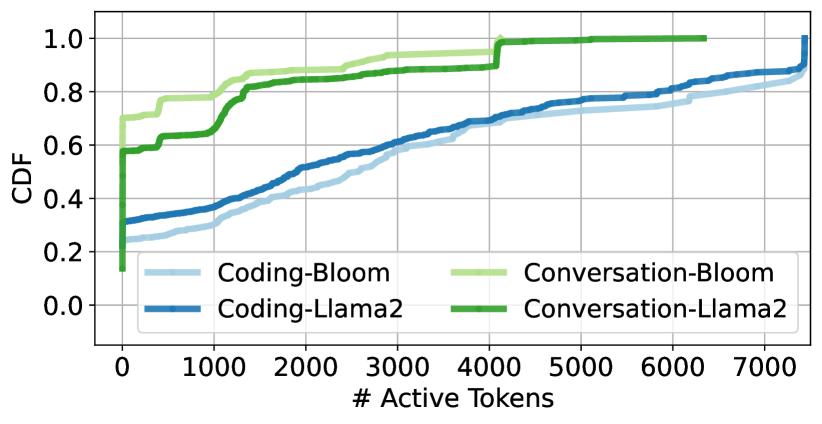
Figure 5 shows the distribution of the time spent by the machine running various numbers of active tokens in a batch. Note that if a prompt of 100 tokens is running in its prompt phase, we count the active tokens as 100. However, once the request is in the token phase, we count it as one active token, since the tokens are generated serially, one at a time (assuming a beam search of one [27]). We find that most of the time (60–70%) for conversation is spent running only 20 tokens or less. Since the coding service has very few output tokens, it experiences even worse batching in the token phase and runs with a single token for more than 20% of the time. Both the LLMs show very similar trends.

Insight II: Most of the time with mixed continuous batching is spent in the token phase, with very few active tokens batched.

III-C Latency

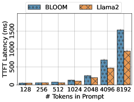
TTFT. Figure 5(a) shows the impact of the number of prompt tokens on TTFT. The range of sizes was chosen based on the coding and conversation traces. We find that TTFT grows almost linearly as the prompt size increases, for both the models. Prompt phase being computationally bound utilizes the GPU-compute well and causes this pattern.

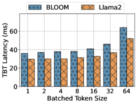
TBT. Figure 5(b) shows the impact of forcefully batching the output tokens of different requests together on TBT. We observe that there is very little impact on TBT as the batch size grows, since the token phase is memory bound. With a batch size of 64, there is only $<2\times$ impact on TBT.

E2E. Figure 5(c) shows various percentiles of E2E latency for coding and conversation traces running on the two models, without any batching. The variability between the request input and output sizes is apparent. Furthermore, we see that most of the E2E time is spent running the token phase of the inference. This is true even for the coding trace, where the prompt size is large, and the generated tokens are few. This further explains the findings in Figure 5. In fact, by our analysis, we find that for BLOOM-176B, a prompt phase with 1500 input tokens takes the same time as token phase with 6 output tokens.

Insight III: For most requests, the majority of the E2E time is spent in the token generation phase.

(a)

(b)

Figure 6: Impact of batching on the throughput for the two LLMs.

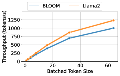
III-D Throughput

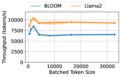
Figure 6 shows the impact of batching on the throughput (measured as tokens per second). For the prompt phase, we define the throughput as the number of prompt input tokens that are processed per second. We see that the throughput decreases after 2048 prompt tokens, which corresponds to a batch size of less than 2 for the median prompt sizes from the traces. On the other hand, Figure 6(b) shows that the throughput in the token phase keeps increasing with batching until 64 batch-size, at which point, the machine runs out of memory.

Insight IV: The prompt phase batch size should be limited to ensure good performance. In contrast, batching the token generation phase yields high throughput without any downside.

Figure 7: Memory requirement with batching in prompt and token phases.

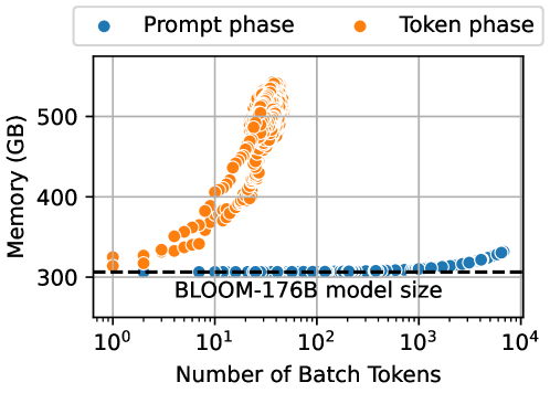
III-E Memory utilization

During an LLM inference, the GPU memory is used to host the model weights and activations, as well as the KV caches (Section II-B). As the number of tokens in a batch increases, the memory capacity requirements for the KV cache also increase. Figure 7 shows the memory capacity utilization during each phase as the number of tokens in the batch increases. During the prompt phase, the active prompt tokens create the KV cache according to their size. During the output token phase, each active generated token that is being processed accesses the KV cache of its entire context so far.

Insight V: Batching during the prompt phase is compute-bound, whereas the token phase is limited by memory capacity.

(a)

(b)

Figure 8: Maximum and mean power utilization varying the batching size.

(a)

(b)

Figure 9: Impact of power cap on the prompt and token generation latency with the maximum batch size possible.

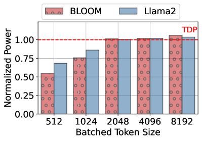
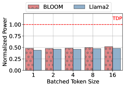
III-F Power utilization

When hosting machines, cloud providers need to consider the peak power draw, which has a direct impact on the datacenter cost [21]. This is especially important when building clusters for GPUs since they consume much higher power than regular compute machines [37, 36]. Figure 8 shows the GPU power draw normalized to the thermal design power (TDP) when running prompt and token generation phases. As the the prompt phase is compute intensive, the power draw increases with the batch size. On the other hand, the token phase is memory bound and the power draw does not vary when increasing the number of tokens to process.

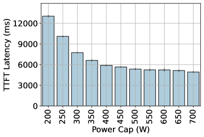
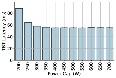
Providers can cap the power usage of the machines to reduce the peak power. Figure 9 shows the impact on latency when increasing the power caps for both prompt and token phases. The prompt phase is highly sensitive to the power cap and the latency increases substantially. On the other hand, the token generation phase sees almost no impact in latency when power capping by over 50% (i.e., 700 to 350W).

Insight VI: While the prompt phase utilizes the power budget of the GPU efficiently, the token phase does not.

	Coding			Conversation
	A100	H100	Ratio	A100	H100	Ratio
TTFT	185 ms	95 ms	0.51$\times$	155 ms	84 ms	0.54$\times$
TBT	52 ms	31 ms	0.70$\times$	40 ms	28 ms	0.70$\times$
E2E	856 ms	493 ms	0.58$\times$	4957 ms	3387 ms	0.68$\times$
Cost [3]	$0.42	$0.52	1.24$\times$	$2.4	$3.6	1.50$\times$
Energy	1.37 Whr	1.37 Whr	1.00$\times$	7.9 Whr	9.4 Whr	1.20$\times$

TABLE IV: P50 request metrics on A100 vs. H100 without batching on Llama2-70B.

III-G GPU hardware variations

Given the different characteristics of prompt and token generation phases, we measure the performance impact on the two from running on different hardware. Table I shows the specifications for DGX-A100 [34] and DGX-H100 [14]. The memory to compute ratio favors A100 compared to H100. Table IV shows our findings. We see a lower performance impact on the token generation phase (TBT) as compared to the Prompt phase (TTFT). Since coding requests are dominated by prompt phase, by having very few generated tokens, the E2E latency impact from A100 is worse on coding than conversation. Furthermore, we see that the overall inference cost and energy are better or equal on A100, compared to H100.

Insight VII: The generation phase can run on cheaper, lower maximum performance hardware for better Perf/W and Perf/$ efficiencies.

IV Splitwise

Based on the insights presented in Section III, we propose Splitwise: a technique to split the prompt and generation phases in the LLM inference on to separate machines.

Figure 10 shows the high-level overview of Splitwise. We maintain two separate pools of machines for prompt and token processing. A third machine pool, the mixed pool, expands and contracts as needed by the workload. All the machines are pre-loaded with the model of choice. When a new inference request arrives, the scheduler allocates it to a pair of machines (i.e., prompt and token). The prompt machines are responsible for generating the first token for an input query, by processing all the input prompt tokens in the Prompt phase and generating the KV-cache. The prompt machine also sends over the KV-cache to the token machine, which continues the token generation until the response is complete. We use continuous batching at the token machines, to maximize their utilization. The mixed pool is the only set of machines where mixed batches would apply. We use mixed continuous batching in those machines.

At a lower request rate, we target better latency in Splitwise, while, at a higher request rate, we target avoiding any performance or throughput reduction due to the fragmentation between prompt and token machine pools.

Figure 10: High-level system diagram of Splitwise.

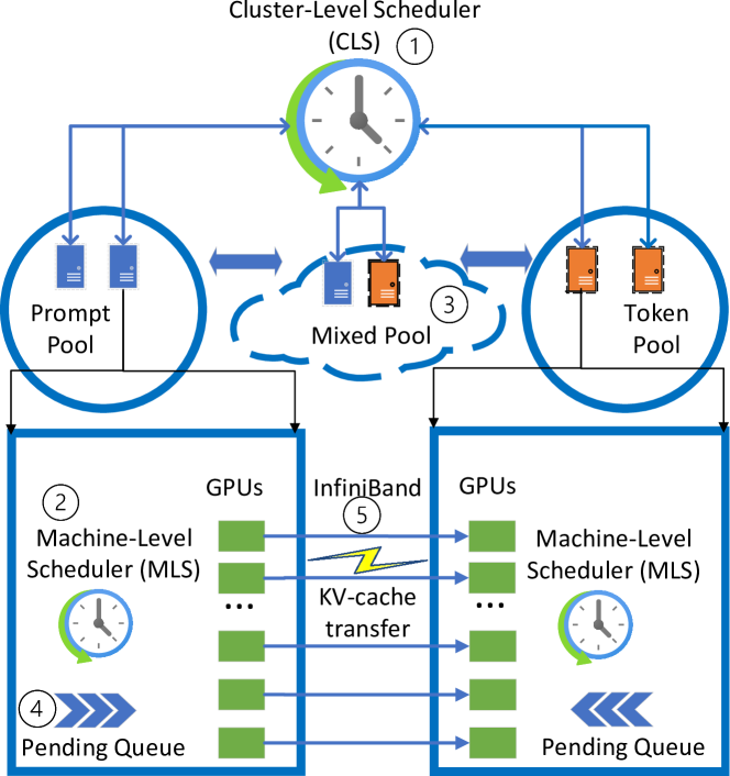
Splitwise uses a hierarchical two-level scheduling as shown in Figure 10. The cluster-level scheduler (CLS) is responsible for routing the incoming requests to particular machines and re-purposing of machines. The machine-level scheduler (MLS) maintains the pending queue and manages batching of requests at each machine.

IV-A Cluster-level scheduling

Request routing. Each machine communicates to the CLS any change in its memory capacity or pending queue. Note that this does not necessarily happen at every single iteration boundary. Then, CLS uses Join the Shortest Queue (JSQ) scheduling [50, 25] to assign a prompt and a token machine to each request upon arrival. We assign the token machine upon arrival to minimize the KV-cache transfer overhead (Section IV-C).

Machine pool management. The CLS mainly maintains two machine pools: the prompt and token pools. Splitwise initially assigns machines to a pool depending on the input/output token distribution and the expected load (i.e., requests per second). If these values deviate considerable from the initial assumptions, Splitwise employs a coarse granularity re-purposing of machines and moves machines between the prompt and token pools. Re-purposing a machine could imply reloading the model (e.g., different degree of parallelism - TP or PP) which can take a significant overhead (e.g., 5 minutes). Therefore, this is done very infrequently if more than 10% of the machines stay in the mixed pool for a long time threshold. The repurposing is performed one-by-one, and during times of lower utilization on the cluster.

Mixed machine pool. To meet SLOs and avoid any performance cliffs due to fragmentation at higher loads, Splitwise maintains a special mixed pool . This pool grows and shrinks dynamically, without any noticeable pool-switching latency, based on the request rates and distributions of input and output tokens. A machine in the mixed pool still retains its original identity as a prompt or token machine and goes back to its original pool once there are no tasks of the opposite kind in its pending queue.

If the CLS tries to assign a prompt and token machine for a request using JSQ and it finds that the queue in the selected machine is beyond a threshold, it looks for target machines in the mixed pool. If the mixed pool is also full, it proceeds to look in the opposite pool (i.e., a token machine to run prompts and vice versa) and moves the machine into the mixed pool. Machines in the mixed pool operate exactly as a non-Splitwise machine would, with mixed batching. Once the queue of mixed requests is drained, CLS transitions the machine back to its original pool. For example, when the queue is too long, we can move a prompt machine to the mixed pool to run tokens; once the machine is done running tokens, we transition the machine back into the prompt pool.

IV-B Machine-level scheduling

The MLS runs on each machine and is responsible for tracking the GPU memory utilization, maintaining the pending queue , selecting the batch size and the batched requests for each iteration, and reporting the relevant status to the CLS.

Prompt machines. The MLS simply uses first-come-first-serve (FCFS) to schedule prompts. The results in Figure 6(a) show that after 2048 prompt tokens, the throughput degrades. For this reason, the MLS restricts the batching of multiple prompts together to 2048 tokens in total. This is a configurable value, and can change for a different model or hardware.

Token machines. The MLS uses FCFS to schedule tokens and batches as much as possible. Figure 6(b) shows that the token generation throughput keeps scaling up with the batch size until the machine runs out of memory. For this reason, the MLS tracks the memory and starts queueing tokens once the machine is close to running out of memory.

Mixed machines. To meet the SLOs for TTFT, the MLS needs to prioritize running prompts and schedules any new prompts in the pending queue immediately. If the machine was running a token phase and there is no capacity, the MLS will preempt tokens. To avoid starvation of the token phase due to preemption, we increase the priority of the token with age and limit the number of preemptions each token can have.

IV-C KV-cache transfer

As discussed in Section II, the KV-cache is generated during the prompt phase of the request, and constantly grows during its token generation phase. In Splitwise, we need to transfer the KV-cache from the Prompt machine to the Token machine (shown in Figure 10) to avoid any duplicate computation. This is the main overhead that Splitwise adds on the LLM inference cluster. In this section, we discuss the impact of KV-cache transfer and how we optimize it.

(a)

(b)

Figure 11: Optimizing KV-cache transfer in Splitwise.

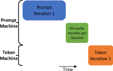
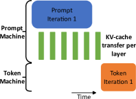
Figure 11(a) shows the Gantt chart for the prompt phase, the KV-cache transfer, and the token generation phase for a single batch of requests when naively transferring the KV cache in a serialized way. The KV-cache transfer starts only after the prompt phase has finished and the first token is generated. Further, it needs to complete before the next output token can be generated in the token generation phase. This directly impacts the maximum TBT and end-to-end latency of inference.

The time required for the transfer depends on the size of the KV cache (which is directly proportional to the number of prompt tokens) and on the bandwidth of the interconnect between the prompt and the token machines. Even when using fast InfiniBand links between the machines, the overhead for large prompt sizes can easily be a significant fraction of the TBT. We discuss this further in the evaluation in Section V-B.

In Splitwise, we optimize the KV-cache transfer by overlapping it with the computation in the prompt phase. As each layer in the LLM gets calculated in the prompt machine, the KV cache corresponding to that layer is also generated. At the end of each layer, we trigger an asynchronous transfer of the KV-cache for that layer while the prompt computation continues to the next layer. Figure 11(b) shows this asynchronous transfer which reduces the overheads. Layer-wise transfers also allow other optimizations, such as earlier start of the token phase in the token machines, as well as earlier release of KV-cache memory on the prompt machines.

For small prompt sizes, the KV-cache is small and it is unnecessary to pay the overheads of fine-grained layer-wise synchronization required by per-layer transfer. Since the number of tokens in a batch is already known at the start of computation, Splitwise picks the best technique for KV-cache transfer. For small prompts, Splitwise uses serialized KV-cache transfer. On the other hand, for larger prompts sizes, it uses the per-layer transfer.

	Prompt Machine			Token Machine			Prompt-Token
	Type	Cost	Power	Type	Cost	Power	Interconnect Bandwidth
Splitwise-AA	DGX-A100	1.00$\times$	1.00$\times$	DGX-A100	1.00$\times$	1.00$\times$	1$\times$
Splitwise-HH	DGX-H100	2.35$\times$	1.75$\times$	DGX-H100	2.5$\times$	1.75$\times$	2$\times$
Splitwise-HHcap	DGX-H100	2.35$\times$	1.75$\times$	DGX-H100	2.5$\times$	1.23$\times$	2$\times$
Splitwise-HA	DGX-H100	2.35$\times$	1.75$\times$	DGX-A100	1.00$\times$	1.00$\times$	1$\times$

TABLE V: Evaluated Splitwise designs all normalized to DGX-A100

IV-D Provisioning with Splitwise

Type of machines. We primarily propose four variants of Splitwise-based systems: Splitwise-HH, Splitwise-HHcap, Splitwise-HA, and Splitwise-AA. The nomenclature is simply drawn from the first letter representing the Prompt machine type, and the second letter representing the Token machine type. “H” represents a DGX-H100 machine, “A” represents a DGX-A100 machine, and “Hcap” represents a power-capped DGX-H100 machine. Table V shows a summary of the cost, power, and hardware in each of our evaluated systems.

Splitwise-HH uses DGX-H100 for both prompt and token machine pools while Splitwise-AA uses DGX-A100 for both pools. These two variants represent the commonly available setups in providers where machines are homogeneous and interchangeable.

Splitwise-HHcap uses DGX-H100 machines for both prompt and token machines. However, we power cap the token machines down to 70% of their rated power, with each GPU capped by 50% of the power. We propose this design based on Figure 9 and Insight VII (i.e., the prompts phase is impacted by power caps while token has no performance impact with 50% lower power cap per GPU).

Splitwise-HA uses DGX-H100 type for prompt machines and DGX-A100 for the token pool. We choose this configuration based on Table IV, and the Insight VII (i.e., A100s can be more cost- and power-efficient for the token phase).

Number of machines. The LLM inference deployment cluster will need to be sized appropriately with the right number of Prompt and Token machines.

Our methodology involves searching the design space using our event-driven cluster simulator (described in detail in Section V-A). We need to provide (1) the target cluster design (e.g., Splitwise-HA or Splitwise-HHcap), (2) the performance model based on the TTFB and TBT latency for various batch sizes for the specific LLM, (3) a short trace derived from the target prompt and token size distributions for the service (e.g., Figure 3), (4) the SLOs (e.g., Table VI), (5) the constraints (e.g., throughput), and (6) the optimization goal (e.g., minimize cost). Using this information, our provisioning framework searches the space for the desired optimal point. For instance this search with a constraint on maximum achievable throughput and an optimization goal of minimizing cost gives us iso-throughput cost-optimized cluster provisioning across different designs.

Figure 12: Design space for provisioning a Splitwise-HH cluster. Cluster configurations targets a peak throughput of 70 requests per second. The cost-optimal Splitwise-HH configuration is marked with a $\filledstar$ (27 prompt and 3 token machines).

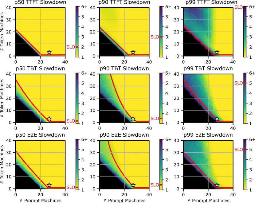
Search space. Figure 12 shows an example of the two-dimensional search space for the number of prompt and token machines for the coding workload (using a 2-minute trace). The simulator outputs the various percentiles for TBT, TTFT, and E2E latencies. Then, we select the cluster size that meets the SLOs on these latencies and optimizes our target function. For example, Figure 12 shows a $\filledstar$ for the setup with the lowest cost that achieves 70 requests per second (RPS). We call this setup iso-throughput cost-optimized.

Optimization. We can use three optimization goals: throughput, cost, and power. Throughput optimization is important for both the cloud service provider (CSP) and the user. The cost optimization has different importance levels to the CSP and the user. For the CSP, a higher cost for the same throughput might be acceptable, if there are gains in power and space for the datacenter. However, for the end-user, a higher cost at the same throughput is generally unacceptable. Finally, the power optimization is attractive for a CSP, since it can allow more GPU deployments in the same datacenter [36], but may not be as important to the user. We only consider the provisioned power for a machine, and not its run time power utilization in this study.

V Evaluation

V-A Methodology

Experimental setup. To evaluate our proposal on real hardware, we build Splitwise for the open-sourced vLLM [27].

Since vanilla vLLM only supports continuous batching with token preemption which can lead to much higher TBT, we implement state-of-the-art mixed continuous batching [48] as discussed earlier in Figure 2(c).

Our implementation of the Splitwise technique assigns machines either a Prompt role, or a Token role. When the prompt machine generates the first token, it transfers the KV-cache to the token machine using the technique described in Section IV-C. We use MSCCL++ [9], an optimized GPU-driven communication library, to implement the naive and layer-wise KV cache transfers. Our implementation considers the contiguity of KV blocks in vLLM to minimize the number of transfers.

We run this modified vLLM on two DGX-A100s and two DGX-H100s full-machine VMs on a public cloud provider with the specifications from Table I. These are the VMs used to collect the characterization data in Section III. These machines are connected with InfiniBand and the DGX-H100s has double the bandwidth (i.e., 400 Gbps).

Simulator setup. While we use the experimental setup to evaluate the Splitwise technique, for the evaluation of the cluster-level design, we would need tens of machines. Instead, we build a simulator to explore the cluster design and evaluate our techniques. The simulator is event-driven and faithfully models the Splitwise machine pools, schedulers, machines-level memory and queues, and KV-cache transfer. For the performance model, we leverage extensive data from experiments on the DGX machines with both models across batches and request sizes. We also feed the performance impact from different prompt and generation phase mixes in a batch.

We use the prompt and token size distributions from the production traces used in Section III. As we increase and decrease the load (requests per second) for cluster sizing, we tune the Poisson arrival rate.

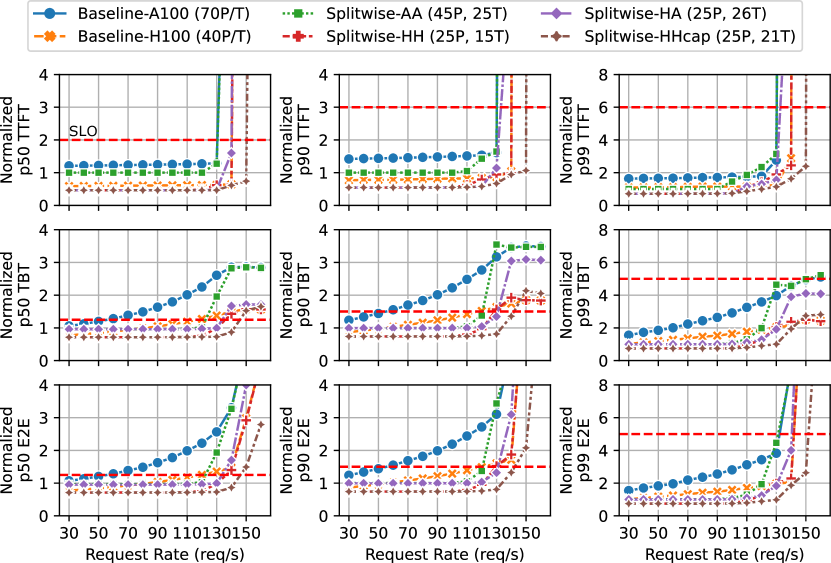
SLOs. To determine the maximum throughput that can be supported by a given cluster design, we use P50, P90, and P99 SLOs for TTFT, TBT, and E2E latency metrics. Table VI shows our SLO definition using DGX-A100 as a reference. We require all nine SLOs to be met. SLOs on TTFT are slightly looser, as it has a much smaller impact on the E2E latency.

	P50	P90	P99
TTFT	2$\times$	3$\times$	6$\times$
TBT	1.25$\times$	1.5$\times$	5$\times$
E2E	1.25$\times$	1.5$\times$	5$\times$

TABLE VI: SLO expressed as slowdown compared to a request running on DGX-A100 under no contention.

Figure 13: Overhead of the KV-cache transfer as the prompt size increases on A100s and H100s machines.

Figure 14: Overhead of KV cache transfer on TTFT, E2E latency for coding trace for H100.

Baselines. We compare our Splitwise designs against Baseline-A100 and Baseline-H100. The clusters in these baselines consist of just DGX-A100s and DGX-H100s respectively. Both baselines use the same optimized mixed continuous batching that Splitwise uses for mixed pool machines (described in Section IV-A).

V-B Experimental results

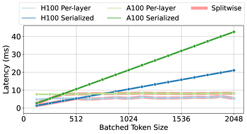
KV-cache transfer latency. We first measure the latency to transfer the KV-cache as the prompt size grows. Figure 13 shows the visible transfer latency on both A100 and H100 setups with the naive and optimized transfer design as discussed in Figure 11. Compared to the prompt computation time, the overhead is minimal ($<7\%$). The time for serialized transfers linearly increases with the prompt size since the size of the KV-cache also increases. The optimized per-layer transfer, on the other hand, hides much of the latency. For these transfers, we see a constant non-overlapped transfer time of around 8ms for the A100 and around 5ms for the H100 setup. The H100 setup has double the bandwidth of the A100 setup (i.e., 200 vs 400 Gbps), and the impact of this can be clearly seen with transfers in the H100 setup happening about twice as fast as those in the A100 setup.

As discussed in Section IV-C, for small prompt sizes ($<512$ in H100), Splitwise uses the serialized KV-cache transfer and for larger prompts, it uses per-layer transfers.

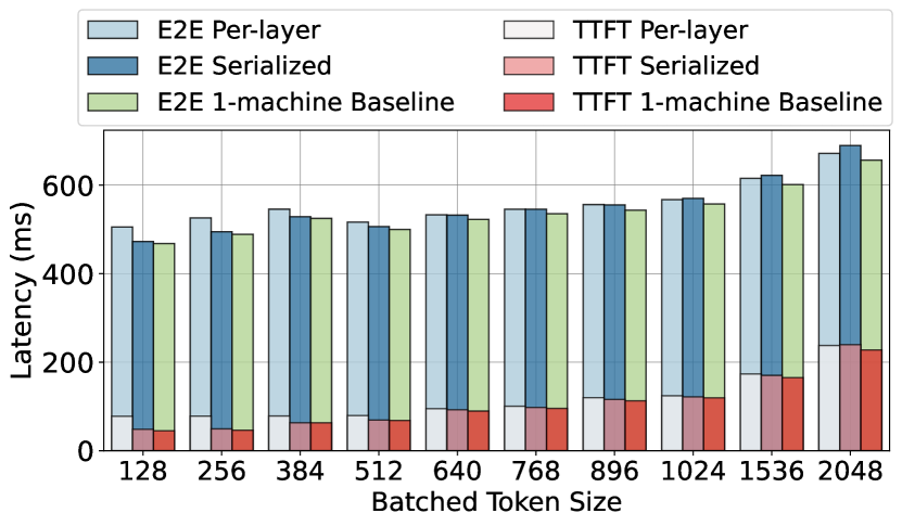
End-to-end impact. Next, we run the coding trace on the 2-machine Splitwise setups without batching, and compare the observed latency metrics to a 1-machine baseline setup with no batching. Figure 14 shows our results. The latency impact of serially transferring the KV-cache grows up to 3% of the E2E with large prompts. However, Splitwise only incurs 0.8% of E2E. In a user-facing inference, the only visible impact of KV-cache transfer overhead is the latency for the second token. Splitwise adds a 16.5% latency to the second token, as compared to the 64% overhead from a serialized transfer. Overall, the transfer impact in Splitwise is hardly perceivable even in a user-facing inference.

V-C Iso-power throughput-optimized clusters

Cluster provisioning. We first provision the clusters using the methodology described in Section IV-D. We target a specific workload (e.g., conversation) at a peak load with the same power (i.e., iso-power) for each cluster design. For the baseline, we use the power for 40 H100 machines as our target peak power ($40\times 700W=28kW$). For the A100 baseline, we require 70 machines ($70\times 400W=28kW$). We denote these two designs as 40P/T and 70P/T as they both use mixed batching in all machines.

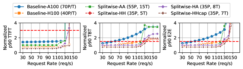
For the Splitwise cluster designs under the coding workload trace, Splitwise-AA provisions 55 prompt machines and 15 for the token pool; denoted as (55P, 15T). Note that similarly to Baseline-A100, Splitwise-AA provisions 75% more machines than Baseline-H100. The legends in Figure 15 show the different provisioning choices under coding and conversation workloads. The design choices for longer token generation is depicted in the machine pool-sizing. For example, we provision more prompt machines for Splitwise-HH (35P, 5T) for the coding trace, while we provision more token machines (25P, 15T) for the conversation trace.

Latency and throughput. Figure 15 shows a deep dive into all the latency metrics at different input load for each cluster design with the same power (i.e., iso-power). For the coding trace (Figure 15(a)), Splitwise-HH, Splitwise-HHcap, and Splitwise-AA all perform better than Baseline-H100. As the load increases, Baseline-H100 suffers from high TBT due to mixed batching with large prompt sizes. Although Splitwise-AA can support higher throughput, its TTFT is consistently higher than most designs. Splitwise-HA clearly bridges the gap by providing low TTFT and E2E at high throughput. The mixed machine pool in Splitwise becomes useful at higher loads to use all the available hardware without fragmentation. This can be clearly seen in the P50 TBT chart for Splitwise-HA, where after 90 RPS, H100 machines jump into the mixed machine pool and help run faster TBT.

For the conversation trace (Figure 15(b)), Splitwise-HHcap clearly does better on all fronts, including latency. This is because the token generation phase runs for much longer than in the coding trace which is beneficial for the token machines.

(a)

(b)

Figure 15: Latency metrics across input loads for iso-power throughput optimized cluster design. The dashed red lines indicate the SLO.

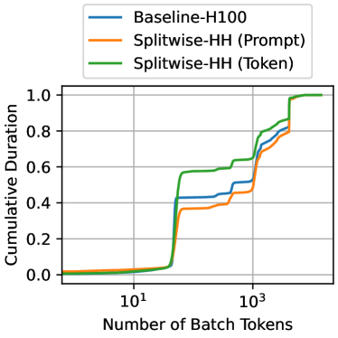
Impact on batched tokens. Figure 16 shows the cumulative distribution of the time spent upto a given number of batched active tokens for a iso-power throughput-optimized cluster running the conversation trace at a low (70 RPS) and a high (130 RPS) load.

At low load, all the 40 Baseline-H100 machines spend 70% of the time running $\leq 15$ tokens, and the rest running mixed batches with large prompts, affecting TBT and E2E. The 35 Splitwise-HH prompt machines are mostly idle, and when active, run much larger batches of tokens. The 15 Splitwise-HH token machines also do a better job at batching. Overall, Splitwise machines have a higher batching and better latency at 70 RPS. At high load, as the mixed pool comes into play, the batch sizes start looking similar across the prompt and token machines.

(a)

(b)

Figure 16: Cumulative distribution of time spent at various batched token sizes for iso-power throughput-optimized design.

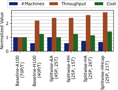
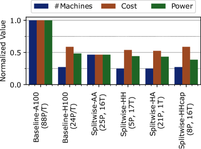
Summary plot. Figure 17(a) summarizes the results across all cluster metrics for iso-power throughput-optimized designs for the conversation trace. We use Baseline-A100 as baseline. Compared to Baseline-A100, Splitwise-AA delivers 2.15$\times$ more throughput at the same power and cost. Compared to Baseline-H100, Splitwise-HA delivers 1.18$\times$ more throughput at 10% lower cost, and the same power.

(a)

(b)

Figure 17: Summary of throughput-optimized cluster designs.

(a)

(b)

Figure 18: Summary of iso-throughput cluster designs.

V-D Other cluster optimizations

We have described iso-power throughput-optimized clusters in detail. For the rest of the cluster optimization evaluation, we only discuss the summary plots.

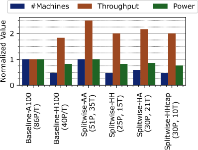
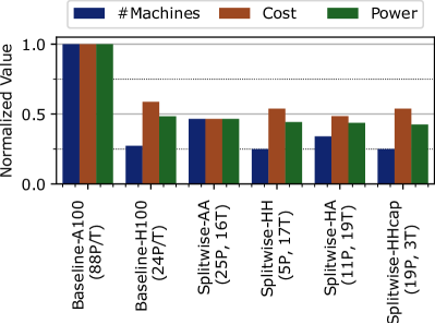
Iso-cost throughput-optimized. Figure 17(b) shows the summary plot for iso-cost clusters, with their space, throughput, and power requirements. We find that Splitwise-AA gives the best throughput for the same cost, namely 1.4$\times$ more throughput than Baseline-H100, running at 25% more power, and 2$\times$ the space. This is an interesting data point, since most customers may not care about power and space, and prefer the 40% extra throughput using older, more easily available GPUs. Whereas the answer for the CSP is not as clear.

Iso-throughput power-optimized. Figure 18(a) shows cluster designs yielding same throughput at the least power. Splitwise-HHcap can achieve the same throughput as Baseline-H100 at 25% lower power at the same cost and space. This can be a clear win for the CSPs.

Iso-throughput cost-optimized. Figure 18(b) shows the cost-optimized versions of the iso-throughput design. Note that there are no changes to any of the homogeneous designs between Figure 18(a) and Figure 18(b). This is because the prompt and token machines have the same cost and power. Splitwise-HA and Splitwise-HHcap though, arrive at slightly different results with the cost and power optimizations. Figure 18(b) shows that with Splitwise-AA, customers can achieve the same throughput as Baseline-H100, at 25% lower cost.

(a)

(b)

Figure 19: Latency impact of running a workload on a cluster designed for another workload. The dashed red lines indicate the SLO.

V-E Impact of workload changes

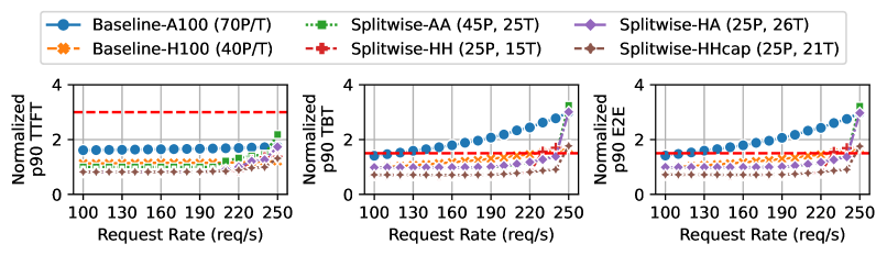
So far, we have tested a trace and a model on clusters optimized for a specific workload pattern and model. To test the robustness of Splitwise, we now run conversation trace on a cluster meant for coding service, and Llama2-70B on a cluster meant for BLOOM-176B. Figure 19 shows these results for iso-power throughput-optimized clusters.

Changing workload trace. Compared to Figure 15(b), we find that in Figure 19(a), the Baseline clusters are similarly sized and see no throughput or latency impact. Splitwise-AA and Splitwise-HH with the mixed pool based scheduling morph well to meet the requirements of the new workload, and see no throughput or latency impact. Since Splitwise-HA and Splitwise-HHcap have different types of machines for Prompt and Token, they experience a throughput setback of 7% from the respective cluster optimized designs for conversation trace. Note that all the Splitwise designs still perform much better than any of the Baseline designs.

Changing model. Figure 19(b) shows that Llama2-70B can support much higher throughput in the same cluster design than BLOOM-176B, given its fewer parameters (Table III). All the Splitwise designs out-perform both the Baseline designs at higher load. Furthermore, Splitwise-HH and Splitwise-HHcap consistently achieve the best latency, even as the load increases.

Summary. Based on these two experiments, we conclude that Splitwise can morph according to the requirements of the workload using its smart scheduling, and is robust to changes in the LLM models, load, and token distributions.

V-F Cluster design for batch job

We design various clusters with Splitwise under strict latency SLOs, even when we are optimizing for throughput. This might not be necessary for batch jobs, that can be stressed to high load, while measuring the generation throughput without latency requirements. We find that upon stressing our iso-power throughput-optimized clusters, Baseline-A100 and Splitwise-AA have the best throughput per cost at 0.89 RPS/$. At high load, Splitwise devolves into the iso-count Baseline, since it starts mixed batching with all the machines in the mixed pool. The same holds true for Splitwise-HH and Baseline-H100, that achieve 0.75 RPS/$.

VI Discussion

Other hardware for the token phase. In this work, the only hardware variants we use are A100 and H100. However, given the token phase characteristics, GPUs like AMD MI-250 [1] and CPUs like Intel Sapphire-Rapids (with HBM) [7] could be effective token machines due to their high memory capacities and bandwidths.

What would optimized hardware look like? Based on our characterization, the prompt phase would need high compute capability with high enough memory bandwidth, but not necessarily a lot of memory capacity. The token phase would need high-enough compute capacity with high memory capacity and bandwidth. Splitwise enables this hardware design space exploration for each phase independently.

Interconnect between prompt and token machines. In this work, we assume Infiniband connection between the prompt and token machines in all the designs (albeit, lower bandwidth when A100s were involved). Although this is common in almost all cloud environments, one of the designs, Splitwise-HA might not be readily available with an Infiniband connection between H100s and A100s machine pools, even though technically feasible. The alternative could be HPC clouds, with Infiniband connections through the CPU [2], or ethernet, using RoCE [33]. Given our optimized KV-cache transfer in smaller blocks utilizing less bandwidth and reducing critical latency however, an interconnect with $10\times$ less bandwidth would still be beneficial. To further reduce our bandwidth utilization, we could also compress the KV-cache before transferring it across the network [30].

Heterogeneous prompt/token machines. Although Figure 19 shows that the mixed-pool based scheduling of Splitwise makes it amenable to varied models and input traces, we recognize that fragmenting a datacenter with different types of GPUs may bring its own challenges for the CSP.

Conversation back and forth. Chat APIs for LLMs today require the user to send the complete context of the conversation so far [15]. However, in the future, services may have enough GPU capacity to cache the context and avoid recomputation. This could sway the memory utilization pattern of the prompt phase from our characterization. Furthermore, it may require transferring the KV-cache back to a prompt machine to be ready for the next conversation request.

VII Related Work

LLM serving. LLM inference serving is a fast developing area, with several recent works optimizing the batching, caching and scheduling [48, 23, 20, 28, 27, 19, 39, 18, 47, 44]. Several prior works have also proposed using CPUs and devices with lower compute capability [6, 10]. However, all the prior work uses the same machine for prompt and token phases. With Splitwise, these systems could benefit by increasing throughput due to phase splitting.

Heterogeneous scheduling. Much prior work exists in the field of heterogeneous scheduling for interactive services [49, 38, 26]. These efforts typically exploit hardware heterogeneity to strike a desirable balance across multiple user and/or CSP objectives such as cost, energy, and performance. Splitwise currently leverages mixed pools for better scheduling, and we plan to explore other scheduling techniques in our future work.

VIII Conclusion

In this work, we extensively characterized the prompt and token generation phases of LLM inference and highlighted the difference in their system utilization patterns. Based on insights from the characterization, we designed Splitwise, which enables separate machines to run the two phases and increases utilization. It opens up a new exploration space as the machine pools for the two phases can be designed and scaled separately. We explored Splitwise designs optimized for throughput, cost, and power, and demonstrated that it performs well even as workloads change. We show that with Splitwise under latency SLOs, we can achieve $1.76\times$ better throughput with 15% lower power at the same cost, or $2.35\times$ better throughput with same cost and power.