Dataset Distillation via the Wasserstein Metric

Abstract

Dataset distillation (DD) offers a compelling approach in computer vision, with the goal of condensing extensive datasets into smaller synthetic versions without sacrificing much of the model performance. In this paper, we continue to study the methods for DD, by addressing its conceptually core objective: how to capture the essential representation of extensive datasets in smaller, synthetic forms.

We propose a novel approach utilizing the Wasserstein distance, a metric rooted in optimal transport theory, to enhance distribution matching in DD. Our method leverages the Wasserstein barycenter, offering a geometrically meaningful way to quantify distribution differences and effectively capture the centroid of a set of distributions. Our approach retains the computational benefits of distribution matching-based methods while achieving new state-of-the-art performance on several benchmarks.

To provide useful prior for learning the images, we embed the synthetic data into the feature space of pretrained classification models to conduct distribution matching. Extensive testing on various high-resolution datasets confirms the effectiveness and adaptability of our method, indicating the promising yet unexplored capabilities of Wasserstein metrics in dataset distillation.

I Introduction

In recent years, dataset distillation [1, 2] has emerged as a topic of growing interest within the computer vision community. It aims to generate a compact synthetic dataset from a training dataset, therefore, the model trained on this synthetic set can achieve performance comparable to one trained on the original set. This modern technique promises to alleviate the issue of increasing model training costs due to the rapid growth of available data, thus facilitating wider experimentation for researchers to develop new models in various application scenarios [3, 4, 5, 6].

Following the promises and the goal of dataset distillation (DD), the central question is about how to capture the essence of an extensive dataset in a much smaller, synthetic version. This process is not merely about the reduction of the data volume, but about distilling the core representation of the dataset itself: to summarize the vast amount of information and condense it into a few, yet most representative samples of the rich distributional information described by the original entire dataset. This concept has driven various innovative approaches in the field. Techniques like gradient matching [2, 7], trajectory matching [8], and curvature matching [9] are some of the methods researchers have explored. These methods, usually viewed as a bi-level optimization problem [10, 11, 12], are particularly focused on aligning the synthetic data closely with specific statistical characteristics of the original, larger dataset.

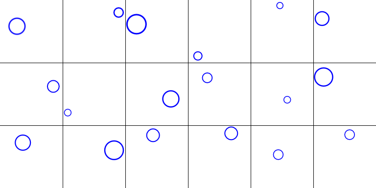
(a)

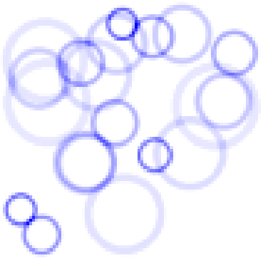
(b)

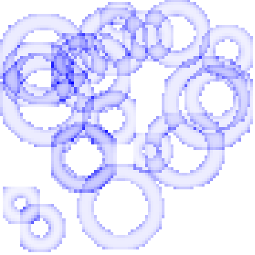
(c)

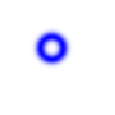
(d)

Figure 1: The capability of Wasserstein barycenter in condensing the core idea of samples: (a) shows some distributions, each of which is uniform on a circle. We consider several such distributions, weight them arbitrarily, and then aim to find their barycenter (centroids) with different approaches: (b) centroids from Euclidean distance (c) centroids from Kullback-Leibler divergence (d) Wasserstein barycenter

There are also other methods that aim to directly align the distributions between synthetic data to the original dataset [13, 14], usually based on the Maximum Mean Discrepancy (MMD) metric [15, 16]. While these methods are often more intuitive to understand (as a direct alignment of distributions), they seem to underperform in comparison to the bi-level optimization methods. We conjecture that a reason behind this undesired performance is the incompetence of MMD metric as a metric to describe the differences between distributions.

Thus, a more powerful metric is naturally expected to improve the performance. We notice the impressive performance of the Wasserstein distance in measuring the differences between distributions. Rooted in optimal transport theory [17], Wasserstein distance measures the minimal movement distance required to transform one probability distribution to another on a given metric space, offering a principled and geometrically meaningful approach to quantify the difference between two distributions. Building upon that, the Wasserstein barycenter [18] was proposed to depict the centroid of a set of distributions in the space of distributions, analogous to the centroid of points in Euclidean space. The impressive performance of Wasserstein barycenter in capturing the essence of samples is shown in Figure 1.

Motivated by this impressive performance, in this paper, we introduce a distinctive distillation method that utilizes the Wasserstein distance for distribution matching. Unlike prior work using the MMD metric [15, 16], the Wasserstein barycenter [18] does not rely on heuristically designed kernels and can naturally take into account the geometry and structure of the distribution. This allows us to statistically summarize the empirical distribution of the real dataset within a fixed number of images, which are representative and diverse enough to cover the variety of real images in each class, to equip a classification model with higher performance.

Further, to address the challenges brought by high-dimensional data optimization, we follow the method in SRe²L [19] to embed the synthetic data into the feature space of a pre-trained image classification model, and further match the real data distribution using BatchNorm statistics [20]. By employing an efficient algorithm [21] to compute the Wasserstein barycenter [18], our method preserves the efficiency benefits of distribution matching-based methods [13] and can scale to large, high-resolution datasets like ImageNet-1k [22]. Experiments show that our method achieves SOTA performance on various benchmarks, validating the effectiveness of our approach.

The salient contributions of our work include:

• A novel dataset distillation technique that integrates distribution matching [13] with Wasserstein metrics, representing an intersection of dataset distillation with the principles of optimal transport theory.

• By leveraging the Wasserstein barycenter [18] and an efficient distribution matching method [13], we have crafted a solution that balances computational feasibility with improved synthetic data quality. This approach is validated by extensive experiments across various high-resolution datasets, demonstrating its effectiveness.

• Comprehensive experimental results across diverse high-resolution datasets. These results highlight the robustness and effectiveness of our approach, showing notable improvements in synthetic data generation and model performance when compared to existing methods. This extensive testing not only demonstrates the practical applicability of our method but also establishes new benchmarks in the field.

The remainder of this paper is organized as follows: Section II introduces related work. Section III elucidates the motivation and design of our method with necessary background on Wasserstein metrics. Section IV describes our experimental framework and results, and the implications of our findings. Section V concludes our paper with potential directions for future research.

II Related Work

II-A Data Distillation

Dataset Distillation (DD) [23] is the process of creating a compact, synthetic training set that enables a model to perform similarly on real test data as it would with a larger, actual training set. Previous DD methods can be divided into three major categories[24]: Performance Matching seeks to minimize loss of the synthetic dataset by aligning the performance of models trained on synthetic and original datasets, methods include DD[23], FRePo[25], AddMem[26], KIP[12], RFAD[11]; Parameter Matching is an approach to train the same neural network using both real and synthetic datasets, with the aim to promote consistency in thier parameters, methods include DC[2], DSA[7], MTT[8], HaBa[27], FTD[28], TESLA[29]; Distribution Matching aims to obtain synthetic data that closely matches the distribution of real data, methods include DM[13], IT-GAN[30], KFS[31], CAFE[14], SRe²L[19].

II-B SRe²L

Most relevant to our work is the SRe²L [19] method. It presents a dataset condensation framework that effectively disentangles the bi-level optimization [10, 11, 12] of model and synthetic data during training. This decoupling enables the handling of datasets of varying scales, diverse model architectures, and differing image resolutions, making it a versatile and effective technique for dataset condensation. It introduces a tripartite learning paradigm comprised of three stages:

Squeeze Involves standard training of a neural network on the original dataset.

Recover Generates synthetic images by optimizing random noise to match the model’s predictions and Batch Normalization statistics from the Squeeze stage. The loss function includes cross-entropy for Softmax prediction alignment, Batch Normalization consistency, and optional image priors (e.g., L2 norm).

Relabel Employs the squeezed model to predict soft labels [32] for multi-crop versions of recovered images, aligning them with true dataset label distributions.

III Method

This section discusses the method employed in our work. We begin by giving an overview of the Wasserstein distance and its direct connection to dataset distillation. Next, we explain the reasons behind our method’s creation and go into its detailed design.

III-A Wasserstein Barycenter in Dataset Distillation

A key component in our method is the computation of representative features using the Wasserstein Barycenter [18]. This concept from probability theory and optimal transport extends the idea of the mean to probability distributions. It calculates a central distribution, effectively summarizing a collection of input probability distributions while considering the geometry of the distribution space.

The Wasserstein Barycenter is aiming to efficiently redistribute one mass distribution into another. This process involves minimizing the Wasserstein distance, also known as the Earth Mover’s Distance.

The effectiveness of the Wasserstein barycenter in summarizing sets of input probability distributions while respecting their geometric structure is well-documented ([33], [21]). We further demonstrate this idea in Figure 1 by considering distributions uniformly spread on circles (Figure 1(a)). When computing their barycenters, methods minimizing Euclidean distance (Figure 1(b)) or using Kullback-Leibler divergence (Figure 1(c)) produce barycenters that do not adequately capture the input distributions’ essence. In contrast, the Wasserstein barycenter (Figure 1(d)) retains the input distributions’ geometric properties, demonstrating its superiority in such tasks.

Computing the Wasserstein Barycenter is typically modeled as a large-scale linear programming (LP) problem. Classical methods like the simplex and interior point methods become inefficient with large distributions [34] or numerous support points. There are significant challenges in computing exact Wasserstein Barycenters due to its NP-hard nature [35], even in relatively simple scenarios.

Innovative algorithms have been developed to approximate Wasserstein Barycenters with reduced computational complexity. Cuturi and Doucet [21] introduced a smoothening approach using an entropic penalty to overcome the computational inefficiency of traditional methods. Our work employs their algorithm for computing free support Wasserstein barycenters, which are not constrained by predefined support. Further advancements in this field include methods for estimating barycenters over continuous spaces [36], stochastic sampling and approximation techniques [37], and adaptations of the alternating direction method of multipliers [34].

III-B Wasserstein Barycenter and Its Computation

Definitions

The Wasserstein distance also referred to as the Earth Mover’s Distance, offers a rigorous metric to quantify the dissimilarity between two probability distributions. This metric has garnered increasing attention in the machine learning realm.

Definition 1 (Wasserstein Distance): For probability distributions $\mu$ and $\nu$ on a metric space $\Omega$ endowed with a distance metric $D$, the $p$-Wasserstein distance is given by

$$W_{p}(\mu,\nu)\stackrel{{\scriptstyle\text{def}}}{{=}}(\inf_{\pi\in\Pi(\mu,\nu)}\int_{\Omega^{2}}D(x,y)^{p}d\pi(x,y))^{\frac{1}{p}}$$

Here, $\mu$ and $\nu$ are the distributions we aim to find the distance between. The space of all such distributions on $\Omega$ is denoted by $P(\Omega)$. $D(x,y)$ represents the distance between any two points $x$ and $y$ in $\Omega$. The collection $\Pi(\mu,\nu)$ denotes the set of all couplings or joint distributions $\pi$ on $\Omega\times\Omega$ that have $\mu$ and $\nu$ as marginals. The symbol $\inf_{\pi\in\Pi(\mu,\nu)}$ represents the infimum over all such transport plans. The Wasserstein distance quantifies the minimum “work” required to rearrange $\mu$ into $\nu$, with the “effort” of moving each mass unit captured by the $p$-th power of the distance $D$.

For the notion of central tendency among a collection of distributions in the Wasserstein space, we introduce the concept of Wasserstein Barycenters.

Definition 2 (Wasserstein Barycenters): For a collection of $N$ distributions ${\nu_{1},\dots,\nu_{N}},\text{in},\mathbb{P}\subset P(\Omega)$, a Wasserstein barycenter is the distribution that minimally averages the $p$-Wasserstein distance to each of these given distributions. Formally, it is the solution to the optimization problem:

$$\arg\min_{\mu\in\mathbb{P}}f(\mu)\quad\text{where}\quad f(\mu)\stackrel{{\scriptstyle\text{def}}}{{=}}\frac{1}{N}\sum_{i=1}^{N}W_{p}^{p}(\mu,\nu_{i})$$

Here, $\mathbb{P}$ represents a subset of the distributions in $P(\Omega)$, and the term $W_{p}^{p}(\mu,\nu_{i})$ denotes the $p$-Wasserstein distance to the power of $p$ between distribution $\mu$ and each distribution $\nu_{i}$ in the collection. In essence, the Wasserstein barycenter symbolizes an “average” distribution in the Wasserstein space, relative to the given collection of distributions.

Computation

To compute the Wasserstein Barycenter given a collection of distributions, we employ the free-support Wasserstein Barycenter computation algorithm proposed by Cuturi and Doucet which uses an alternating optimization scheme [21]. To alleviate the substantial computational costs and slow convergence rates associated with the optimal transport problem for computing the Wasserstein Barycenter, a smoothening approach is used by introducing an entropy regularisation

To obtain the relative importance of each datapoint in the support of the computed barycenter, we introduce a weight associated with each datapoint. To compute these weights, we employ the algorithm for computing fixed support Wasserstein barycenters outlined in [21] (refer to Algorithm 2 in the appendix) to estimate these weights. The complete framework involves the joint optimization of both the datapoints in the support of the Wasserstein barycenter, and the corresponding weights assigned to them.

III-C Dataset Distillation and the Wasserstein Barycenter

Let $\mathcal{T}=\{\mathbf{x}_{i},y_{i}\}_{i=1}^{n}$ denote the real dataset and $\mathcal{S}=\{\tilde{\mathbf{x}}_{i},\tilde{y}_{i}\}_{i=1}^{m}$ denote the synthetic dataset. Dataset Distillation (DD) can be formulated as a bi-level optimization problem as:

$$\min_{\mathcal{S}} \sum_{i=1}^{n}\ell(f(\mathbf{x}_{i};\boldsymbol{\theta}(\mathcal{S})),y_{i})$$

subject to $$\boldsymbol{\theta}(\mathcal{S})=\operatorname*{arg\,min}_{\boldsymbol{\theta}}\sum_{i=1}^{m}\ell(f(\tilde{\mathbf{x}}_{i};\boldsymbol{\theta}),\tilde{y}_{i})$$ (1)

where $f(\cdot;\boldsymbol{\theta})$ denotes a model parametarized by $\boldsymbol{\theta}$, and $\ell(\cdot,\cdot)$ is a loss function.

Navigating the intricacies of the bi-level optimization problem poses significant challenges. As a viable alternative, a prevalent approach [13, 14, 38, 19] seeks to align the distribution of the synthetic dataset with that of the real dataset. This strategy is based on the assumption that the optimal synthetic dataset should be the one that is distributionally closest to the real dataset subject to a fixed number of synthetic data points. While recent methods grounded on this premise have shown promising empirical results, they have not yet managed to bridge the performance gap with the state-of-the-art techniques.

Given the intuitive design of Wassertein distance as a metric to describe the distances between distributions, and its strong empirical performances Fig 1, we believe the strengths of Wassertein distance can boost the performance to bridge the gap and even surpass the SOTA techniques.

To begin with, we represent both the real and synthetic dataset as empirical distributions. With no prior knowledge about the samples in the real dataset, it is common to assume a discrete uniform distribution over the observed data points. Consequently, the empirical distribution of the real dataset $\mathcal{T}$ is:

$$\mu_{\mathcal{T}}=\frac{1}{n}\sum_{i=1}^{n}\delta_{\mathbf{x}_{i}},$$ (2)

where $\delta_{\mathbf{x}_{i}}$ denotes the Dirac delta function centered at the data point $\mathbf{x}_{i}$. $\mu_{\mathcal{T}}$ is defined on the set $\mathcal{P}_{n}$ of probability distributions that are supported by at most $n$ points in $\mathbb{R}^{d}$, where $n$ represents the size of the real dataset and $d$ denotes the input dimension.

For the synthetic dataset $\mathcal{S}$, its empirical distribution is:

$$\mu_{\mathcal{S}}=\sum_{i=1}^{m}a_{i}\delta_{\tilde{\mathbf{x}}_{i}}$$ (3)

where $\sum_{i=1}^{m}a_{i}=1$ and each $a_{i}\geq 0$. The probability can be learned to allow more flexibility. $\mu_{\mathcal{S}}$ is defined on the set $\mathcal{P}_{m}$ of probability distributions that are supported by at most $m$ points in $\mathbb{R}^{d}$.

Based on our above-mentioned assumption and chosen metric, the optimal synthetic dataset $\mathcal{S}^{*}$ should generate an empirical distribution which is the barycenter of the original real dataset $\mathcal{T}$,

$$\mu_{\mathcal{S}}^{*}=\operatorname*{arg\,min}_{\mu_{\mathcal{S}}\in\mathcal{P}_{m}}W_{p}(\mu_{\mathcal{S}},\mu_{\mathcal{T}})$$ (4)

where $W_{p}$ is the Wasserstein distance. This positions the dataset distillation process as a search for the Wasserstein Barycenter of the empirical distribution derived from $\mathcal{T}$.

1

Input: Real dataset $\mathcal{T}=\{\mathbf{x}_{c,n}\}_{n=1,\ldots,N}^{c=1,\ldots,C}$

2

3Train a teacher model $f$ on $\mathcal{T}$;

4

5for each class $c$ do

6       for each sample $n$ do

7             Perform forward pass: $f(\mathbf{x}_{c,n})$;

8             Store feature: $f_{e}(\mathbf{x}_{c,n})$;

9            

10      Compute $\text{BN}_{c,l}^{\text{mean}}$, $\text{BN}_{c,l}^{\text{var}}$;

11      

12

13for each class $c$ do

14       $\{\mathbf{b}_{c,m}\}_{m=1,\ldots,M}\leftarrow\operatorname{barycenter}\left(\{f_{e}(\mathbf{x}_{c,n})\}_{n=1,\ldots,N}\right)$ according to Algorithm 3 in the Appendix;

15      

16      Optimize $\{\tilde{\mathbf{x}}_{c,m}\}_{m=1,\ldots,M}$ according to Equation 7;

17      

18

Output: Synthetic dataset $\mathcal{S}=\{\tilde{\mathbf{x}}_{c,m}\}_{m=1,\ldots,M}^{c=1,\ldots,C}$

Algorithm 1 Dataset Distillation via the Wasserstein Metric

III-D Wasserstein Metric-Based Dataset Distillation

While the above gives a conceptual discussion, it is in practice not viable to use the barycenter at the pixel level as synthetic data. Since natural images are sparsely distributed in a high dimensional space, it is necessary to use some prior knowledge to learn synthetic images that encode meaningful information from the real dataset. The SRe2L method effectively leverages the knowledge in a pretrained image classifier to recover a condensed version of training data. Extending this idea, we use a pretrained classifier to embed the images into the feature space, in which we compute the Wasserstein barycenter to learn synthetic images. Our method essentially improves upon the recover stage of SRe²L for more explicit and principled distribution matching, while keeping other stages the same for controlled comparison. We describe our method as follows.

Suppose the real dataset $\mathcal{T}$ has $C$ classes, with $N$ images per class. Let us re-index the samples by classes and denote the training set as $\mathcal{T}=\{\mathbf{x}_{c,n}\}_{n=1,\ldots,N}^{c=1,\ldots,C}$. Suppose that we want to distill $M$ images per class. Denote the synthetic set $\mathcal{S}=\{\tilde{\mathbf{x}}_{c,m}\}_{m=1,\ldots,M}^{c=1,\ldots,C}$, where $M\ll n$.

First, we employ the pretrained model to extract features for all samples within each class in the original dataset $\mathcal{T}$. More specifically, we use the pretrained model $f$ to get the features $\{f_{e}\left(\mathbf{x}_{c,n}\right)\}_{n=1,\ldots,N}$ for each class $c$, where $f_{e}(\cdot)$ is the function that produces the final features before the linear classifier.

Next, we compute the Wasserstein barycenter for each set of features computed in the previous step. We treat the feature set for each class as an empirical distribution, and apply the algorithm in [21] to compute the free support barycenters with $M$ points for class $c$, denoted as $\{\mathbf{b}_{c,m}\}_{m=1,\ldots,M}$, where $M$ is the predefined number of synthetic samples per class.

Then, in the main distillation process, we employ an iterative gradient descent approach to learn the synthetic images by jointly considering two objectives. On the one hand, we match the features of the synthetic images with the corresponding data points in the learned barycenters:

$$\mathcal{L}_{\text{feature}}(\mathcal{S}) =\sum_{c=1}^{C}\sum_{m=1}^{M}\|f_{e}(\tilde{\mathbf{x}}_{c,m})-\mathbf{b}_{c,m}\|_{2}^{2}.$$ (5)

where $f_{e}(\cdot)$ is the function to compute features of the last layer.

On the other hand, it is empirically beneficial for the synthetic images to be situated closely to the manifold of real images. To encourage this, previous works [39, 19] have used BatchNorm statistics on the real dataset to align the feature map distribution of the synthetic data. To better capture the intra-class distribution of the real data, we refine this approach to compute the per-class BatchNorm statistics of the real data, and regularize the synthetic images of each class separately. More specifically, we employ the below loss function for regularizing the synthetic set $\mathcal{S}$:

where $L$ is the number of BatchNorm layers, and $f_{l}(\cdot)$ is the function that computes intermediate features as the input to the $l$-th BatchNorm layer. $\mathcal{A}_{\text{mean}}(\cdot)$ and $\mathcal{A}_{\text{var}}(\cdot)$ are the aggregate operators in a standard BatchNorm layer, which compute the per-channel mean and variance of the feature map of the synthetic data. ${BN}_{c,l}^{\text{mean}}$ and ${BN}_{c,l}^{\text{var}}$ are the mean and variance statistics for class $c$ of the real training set at the $l$-th BatchNorm layer. These statistics are computed with one epoch of forward pass over the training dataset. Our experiments show that per-class BatchNorm statistics result in significantly better performance of the synthetic data.

Combining these objectives above, we employ the below loss function for learning the synthetic data:

$$\mathcal{L}(\mathcal{S})=\mathcal{L}_{\text{feature}}(\mathcal{S})+\lambda\mathcal{L}_{\text{BN}}(\mathcal{S}).$$ (7)

where $\lambda$ is a regularization coefficient.

IV Experiments

TABLE I: Performance comparison of different dataset distillation methods on different datasets.

Methods

ImageNette

Tiny ImageNet

ImageNet-1K

1

10

50

100

1

10

50

100

1

10

50

100

Random [13]

23.5 $\pm$ 4.8

47.7 $\pm$ 2.4

-

-

1.5 $\pm$ 0.1

6.0 $\pm$ 0.8

16.8 $\pm$ 1.8

-

0.5 $\pm$ 0.1

3.6 $\pm$ 0.1

15.3 $\pm$ 2.3

-

DM [13]

32.8 $\pm$ 0.5

58.1 $\pm$ 0.3

-

-

3.9 $\pm$ 0.2

12.9 $\pm$ 0.4

24.1 $\pm$ 0.3

-

1.5 $\pm$ 0.1

-

-

-

MTT [8]

47.7 $\pm$ 0.9

63.0 $\pm$ 1.3

-

-

8.8 $\pm$ 0.3

23.2 $\pm$ 0.2

28.0 $\pm$ 0.3

-

-

-

-

-

DataDAM [38]

34.7 $\pm$ 0.9

59.4 $\pm$ 0.4

-

-

8.3 $\pm$ 0.4

18.7 $\pm$ 0.3

28.7 $\pm$ 0.3

-

2.0 $\pm$ 0.1

6.3 $\pm$ 0.0

15.5 $\pm$ 0.2

-

SRe2L [19]

-

-

-

-

-

-

41.1 $\pm$ 0.4

49.7 $\pm$ 0.3

-

21.3 $\pm$ 0.6

46.8 $\pm$ 0.2

52.8 $\pm$ 0.4

SRe2L(replicated)

20.6 $\pm$ 0.3

54.2 $\pm$ 0.4

80.4 $\pm$ 0.4

85.9

4.0$\pm$ 0.2

38.1$\pm$ 0.2

57.2 $\pm$ 0.2

59.8 $\pm$ 0.4

2.9 $\pm$ 0.2

36.1$\pm$ 0.1

54.4$\pm$ 0.3

58.3$\pm$ 0.3

WMDD (Ours)

40.2 $\pm$ 0.6

64.8 $\pm$ 0.4

83.5 $\pm$ 0.3

87.1

7.6 $\pm$ 0.2

41.8 $\pm$ 0.1

59.4 $\pm$ 0.5

61.0 $\pm$ 0.3

3.2$\pm$ 0.3

38.2 $\pm$ 0.2

57.6$\pm$ 0.5

60.7$\pm$ 0.2

To evaluate the performance of our method, we conducted comprehensive experiments on three high-resolution datasets, namely, ImageNette, Tiny ImageNet, and ImageNet-1K. We evaluated our method under different budges of synthetic images: 1, 10, 50 and 100 images per class (IPC), respectively. We pretrained a ResNet-18 model [40] on the real training set, from which we distilled the dataset following our method, and used the synthetic data to train a ResNet-18 model from scratch. Then, the performance of the synthetic dataset is evaluated by the top-$1$ accuracy of the trained model on the validation set. We report the mean accuracy of the model on the validation set, repeated across 3 different runs. Table I shows our experiment results, as well as the reported results from several recent methods for comparison.

Our implementation of the barycenter algorithm was partly based on the Python Optimal Transport library [41]. We keep most of the hyperparameter settings the same with [19], but set the regularization coefficient $\lambda$ differently to account for our different loss terms. We set $\lambda$ to $500$ for ImageNet and Tiny ImageNet, and $10$ for ImageNette. Additionally, we modified the batch size in the pretraining stage to adapt to our computation environment, and changed another hyperparameter based on our preliminary experiments. This results in large performance improvement when replicating their results. Therefore, we include both their reported results and our replicated results in the table. For more details please see the supplementary materials.

Our method consistently showed SOTA performance in most settings across different datasets. Compared to MTT [8] and DataDAM [38], which show good performance in fewer IPC settings, the performance of our method increases more rapidly with the number of synthetic images. Notably, the top-1 accuracy of our method in the 100 IPC setting are $87.1\%$, $61.0\%$, $60.7\%$, on the three datasets respectively, drawing close to those of the pretrained classifiers used in our experiment, i.e., $89.9\%$, $63.5\%$, and $63.1\%$, each pretrained on the full training set. This superior performance underscores the effectiveness and robustness of our approach in achieving higher accuracy across different datasets.

IV-A Cross-architecture Generalization

Synthetic data often overfit to the model used to learn them, a common issue found in dataset distillation research [42, 43]. To evaluate whether our synthetic datasets can adapt to new architectures not seen in the distillation process, we did experiments using our learned data to train different models that were randomly initialized, and evaluated their performance on the validation set. We used ResNet-18 to learn the synthetic data, and report the performance of different training models, namely ResNet-18, ResNet-50, ResNet-101 [40] and ViT-Tiny [44], in both 10 and 50 IPC settings. The results are shown in Table II. It can be seen that our synthetic data generalize well to other models in the ResNet family, and the performance increases with the model capacity in the settings where the data size is relatively large. Our synthetic dataset shows lower performance on the vision transformer, probably due to its data-hungry property.

TABLE II: Cross-architecture generalization performance on Tiny-ImageNet, and ImageNet in different IPC settings. We used ResNet-18 for distillation, and different architectures for evaluation: ResNet-{18,50,101} and ViT-Tiny with patch size of 16.

Dataset	IPC	Training Model
		ResNet-18	ResNet-50	ResNet-101	ViT-T
Tiny-ImageNet	10	41.8	34.7	35.3	11.7
	50	59.4	60.5	60.7	29.0
ImageNet	10	38.2	43.7	42.1	7.5
	50	57.6	61.3	62.2	30.7

IV-B Ablation study

To identify the design components in our method that contribute to the improved performance, we conduct ablation study on several important variables: whether to include the cross-entropy loss in [19] to maximize the class probability from the pretrained model, whether to include the feature matching loss based on Wasserstein barycenter (Equation 5), and whether to choose standard BatchNorm or per-class BatchNorm statistics for regularization. We experimented these variables on different datasets under the 10 IPC setting. The results in Table III show that compared with the baseline method (Row 5), choosing per-class BatchNorm regularization effectively improves the performance on all datasets (Row 3), and it is best used in combination with our barycenter loss (Row 1). When we additionally use the CE loss (Row 2), the performance does not improve in general, which shows that the distribution matching objectives are enough to learn high-quality datasets.

TABLE III: Ablation study on three variables: whether to include the cross-entropy loss, whether to choose standard BatchNorm or per-class BatchNorm statistics for regularization, and whether to include the feature matching loss based on Wasserstein barycenter (Equation 5).

$\mathcal{L}_{\text{CE}}$	$\mathcal{L}_{\text{BN}}$	$\mathcal{L}_{\text{Bary}}$	ImageNette	Tiny ImageNet	ImageNet-1K
✗	✓	✓	64.8$\pm$ 0.4	41.8$\pm$ 0.1	38.2$\pm$ 0.2
✓	✓	✓	63.9$\pm$ 0.3	42.1$\pm$ 0.5	37.9$\pm$ 0.3
✓	✓	✗	64.0$\pm$ 0.1	41.3$\pm$ 0.4	37.4$\pm$ 0.5
✗	✗	✓	60.7$\pm$ 0.2	36.5$\pm$ 0.2	26.7$\pm$ 0.3
✓	✗	✗	54.2$\pm$ 0.4	38.1$\pm$ 0.2	36.1$\pm$ 0.1

TABLE IV: Synthesis Time and Memory Usage on ImageNette (64×64 resolution) using a single GPU for our method. The ’Time Cost’ indicates the time taken (ms) to generate one image with a single iteration update on synthetic data. The peak GPU memory usage is recorded or estimated for a batch size of 200, considering 1 IPC as the dataset comprises 10 classes.

GPU Type	Condensed Arch	Time Cost (ms)	Peak GPU Memory Usage (GB)
V100	ResNet-18	2.4	0.78

Hyperparameter sensitivity

To better understand the effect of the regularization term in our method, and how the regularization strength affect the performance of our data, we tested a broad range of values for the regularization coefficient $\lambda$. We experimented with $\lambda$ ranging from $10^{-1}$ to $10^{3}$, and evaluated the performance of our distilled data on the three datasets under 10 IPC setting. Fig 2 shows that when $\lambda$ is small, the performance on all three datasets are lower; as $\lambda$ gradually increases, the performance also increases and then keeps relatively stable. This shows that the regularization is indeed useful for learning high-quality datasets, and particularly important to many-class settings.

The effect of regularization can also be seen from manual observation. Fig. 3 shows some exemplar synthetic images of the same class. When $\lambda$ is too small to yield descent performance, the synthetic image contains high-frequency components which may indicate overfitting to the specific model weights and architecture, therefore compromising their generalizability. Synthetic images with a sufficiently large $\lambda$ tend to align better with human perception.

Figure 2: Hyperparameter sensitivity of $\lambda$ on the three datasets.

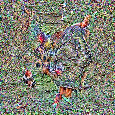
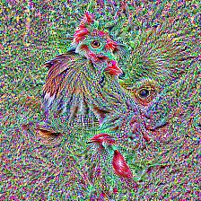
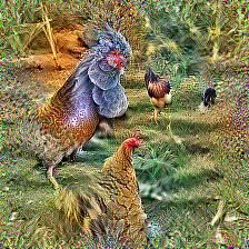
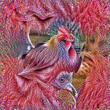
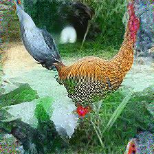
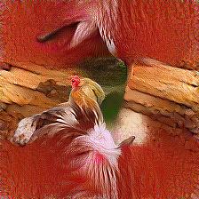
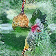
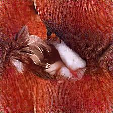
$\lambda$: 0.1 $\lambda$: 1 $\lambda$: 100 $\lambda$: 1000

Figure 3: Visualizations of synthetic images in Imagenet-1k with different $\lambda$

IV-C Feature Embedding Distribution

To see how our synthetic data are distributed relative to the distribution of the real data, we did a visualization analysis. To map the real data and synthetic data into the same feature space, we train a model from scratch on a mixture of both data. Then we extract their last-layer features and use the t-SNE [45] method to visualize their distributions on a 2D plane. For a comparison, we conduct this process for the synthetic data obtained with both our method and the SRe²L method. Fig. 4 shows the result. In the synthetic images learned by the SRe²L method, synthetic images within the same class tend to collapse, and those from different classes tend to be far apart. This is probably a result of the cross-entropy loss they used, which optimizes the synthetic images toward maximal output probability from the pretrained model. On the other hand, our utilization of the Wasserstein metric enables synthetic images to better represent the distribution of real data.

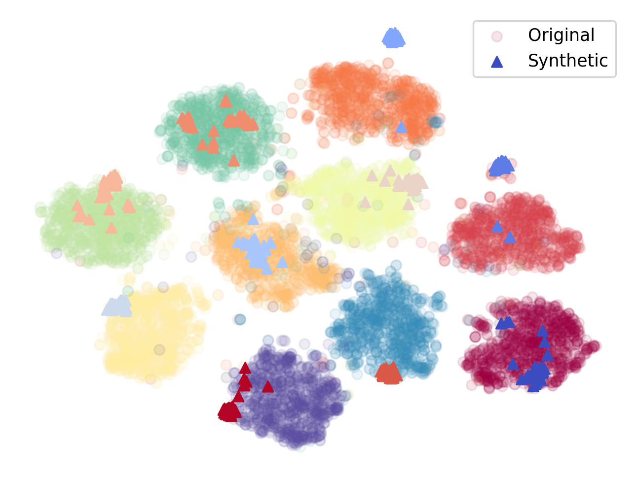
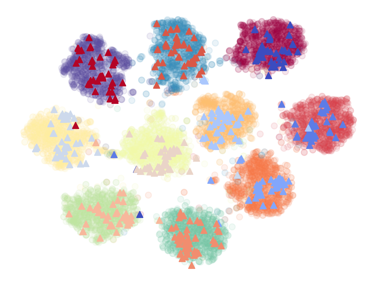
Figure 4: Distribution visualization of ImageNette. The dots presents the distribution of the original dataset using the latent space of a model(ResNet-101[40] in this case) and the triangles are distilled images. The distribution of data distilled using the SRe²L[19] method is shown in the image above and the distribution obtained through our method of distillation is displayed in the image below.

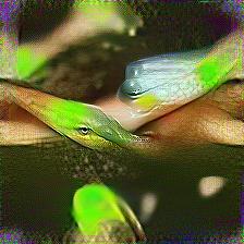
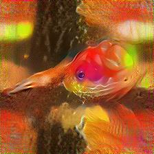
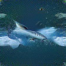
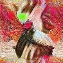
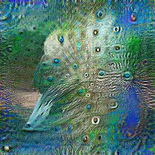
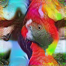
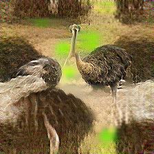
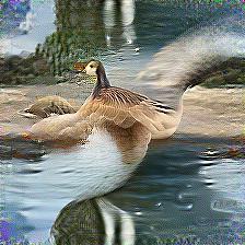
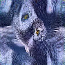
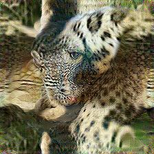
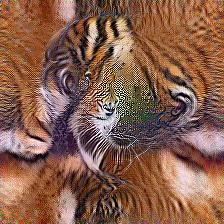
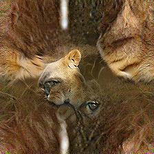
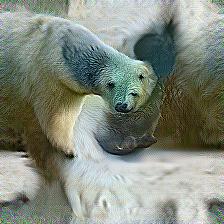
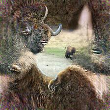
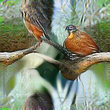
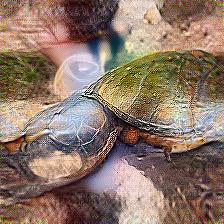
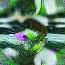
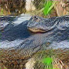
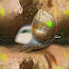
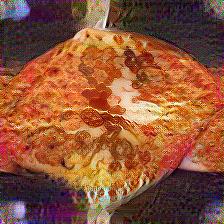
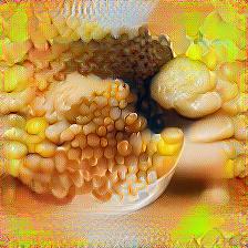
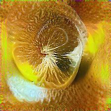
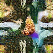
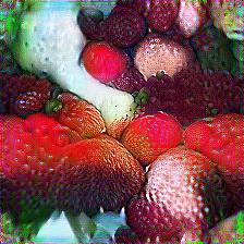
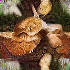
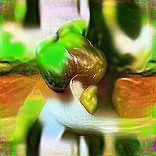
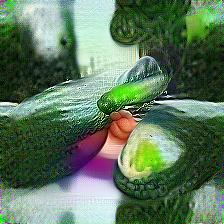
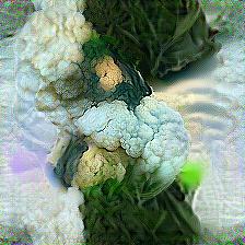
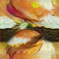
Snake Gold Fish Shark Cock Peacock Macaw Ostrich Goose Flamingo Grey Owl Leopard Tiger Lion Polar Bear Bison Robin Mud Turtle Tree Frog Alligator Snail Pizza Corn Lemon Pineapple Strawberry Mushroom Bell Pepper Cucumber Cauliflower Burger

Figure 5: Visualizations of Our Synthetic Images from ImageNet-1k

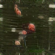
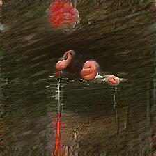
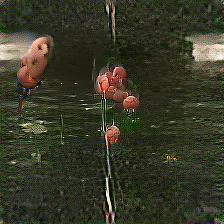
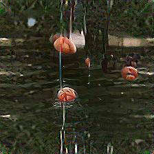
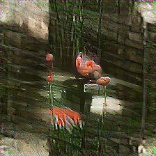
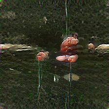
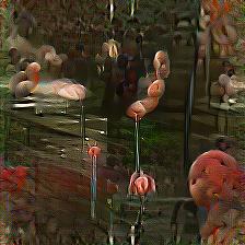
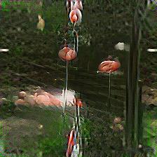
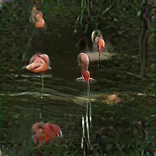
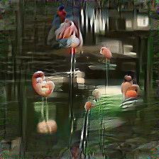
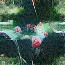
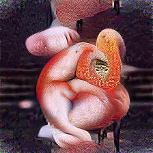
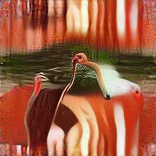
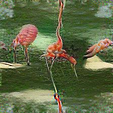
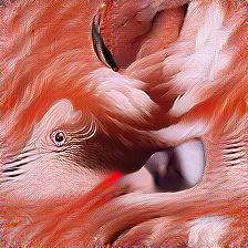
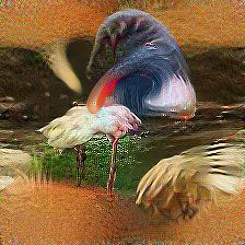
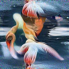
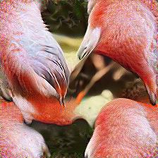
SRe²L synthetic images of class Flamingo (classId: 130) Our synthetic images of the class Flamingo (classId: 130)

Figure 6: Visualizations of our synthetic images vs. SRe²L baseline synthetic images from ImageNet-1k Flamingo class (classId: 130)

IV-D Increased Variety in Synthetic Images

Visualization of the synthetic images at the pixel level corroborates our finding in Section IV-C, with the ImageNet-1k Flamingo class being one such example, as shown in Fig. 6. Compared to the SRe²L baseline synthetic images, our method leads to improved variety in both the background and foreground information contained in synthetic images. The incorporation of the Wasserstein metric in our methodology appears to contribute to this increased variety. By covering the variety of images in the real data distribution, our method prevents the model from relying on a specific background color or object layout as heuristics for prediction, thus alleviating the potential overfitting problem and improving the generalization of the model.

V Conclusion

In conclusion, in this paper, we introduce a new approach to dataset distillation, leveraging the principles of Wasserstein metrics derived from optimal transport theory. This method shows that the perspectives of distribution matching within this area, providing new insights and perspectives. Our methodology effectively narrows the divide between efficiency and performance, offering a powerful solution that adeptly handles high-resolution datasets while maintaining the integrity and quality of data. Through rigorous empirical testing, our approach has demonstrated impressive performance across a variety of benchmarks, highlighting its reliability and practical applicability in diverse scenarios. Our ablation study also supports the design rationales behind the method, suggesting the power of Wasserstein metrics in learning the core representations of the data distributions. This research not only sets a new benchmark in the realm of dataset distillation but also opens up exciting avenues for further investigation into the synergistic relationship between optimal transport theory and machine learning. As we progress, the integration of these two fields holds the promise of groundbreaking developments and innovative breakthroughs in the expansive field of computer vision. This work stands as a testament to the potential of combining theoretical concepts of Wasserstein metrics with practical applications of reducing data volume.

Supplementary Material

A Algorithm details

This section provides the details of the algorithm for barycenter computation [21] used in our method. Consider two sets $X=(x_{1},\ldots,x_{n})$ and $Y=(y_{1},\ldots,y_{m})$ in $\Omega$. For empirical distributions $\mu=\sum_{i=1}^{n}a_{i}\delta_{x_{i}}$ and $\nu=\sum_{i=1}^{m}b_{i}\delta_{y_{i}}$, the Wasserstein distance $W_{p}(\mu,\nu)$ is derived by solving a transportation problem with the following elements:

1. The matrix $M_{XY}$ representing pairwise distances between $X$ and $Y$, raised to power $p$, serving as a cost matrix:

   $$M_{XY}\coloneqq\left[D(x_{i},y_{j})^{p}\right]_{ij}\in\mathbb{R}^{n\times m},$$ (8)

2. The transportation polytope $U(a,b)$ for $a\in\Sigma_{n}$ and $b\in\Sigma_{m}$, where $\Sigma_{n}$ is the probability simplex with $n$ dimensions. $U(a,b)$ defines the feasible set of nonnegative matrices with specific row and column marginals:

   $$U(a,b)\coloneqq\left\{T\in\mathbb{R}_{+}^{n\times m}\mid T\mathbf{1}_{m}=a,T^{\top}\mathbf{1}_{n}=b\right\}$$ (9)

Combining Eq. 8 and 9, the $p$-th power of $W_{p}(\mu,\nu)$ can be formulated as a parametric linear program:

$$W_{p}^{p}(\mu,\nu)=\mathbf{p}(a,b,M_{XY})\coloneqq\min_{T\in U(a,b)}\langle T,M_{XY}\rangle.$$ (10)

For a matrix $M\in\mathbb{R}^{n\times m}$, the optimal $\mathbf{p}(a,b,M)$ can be expressed in a dual Linear Program (LP) form:

$$\mathbf{d}(a,b,M)=\max_{(\alpha,\beta)\in C_{M}}\alpha^{\top}a+\beta^{\top}b,$$ (11)

where $C_{M}$ is the polyhedron of dual variables:

$$C_{M}=\{(\alpha,\beta)\in\mathbb{R}^{n+m}\mid\alpha_{i}+\beta_{j}\leq m_{ij}\}.$$ (12)

The LP duality principle ensures $\mathbf{d}(a,b,M)=\mathbf{p}(a,b,M)$.

Looking for a barycenter $\mu$ with atoms $X$ and weights $a$ is equivalent to minimizing $f$ defined below

$$f(a,X)\coloneqq\frac{1}{N}\sum_{i=1}^{N}\mathbf{p}(a,b_{i},M_{XY_{i}}),$$ (13)

over relevant feasible sets for $a$ and $X$. To solve this, an iterative approach is taken to optimize $a$ with a given $X$ and vice versa.

For a fixed $X$, finding optimal weights $a\in\Theta$ minimizes $f(a,X)$. A subgradient for $f$ w.r.t $a$ can be obtained from the dual optimal solutions of $\mathbf{p}(a,b_{i},M_{XY_{i}})$ [21], allowing for the minimization of $f$ using subgradient-based methods. Then, using a Bregman divergence $B(a,b)$ defined by a prox-function $w$ for $a,b\in\Theta$, we can define the proximal mapping $P_{a}(b)=\operatorname*{arg\,min}_{c\in\Theta}(\langle b,c-a\rangle+B(a,c))$, and leverage accelerated gradient methods [46]. Specifically, we chose the KL Divergence [47] for $B$ in this work. Algorithm 2 shows this process.

For a fixed $a$, finding optimal positions $X$ minimizes $f(a,X)$. Suppose $T^{*}$ is the optimal solution for $\mathbf{p}(a,b,M_{XY})$, the Newton update can be derived for minimizing a local quadratic approximation of $\mathbf{p}$ at $X$:

$$X\leftarrow YT^{\star T}\text{diag}(a^{-1}).$$ (14)

The overall approach for approximating the minimization of $f(a,X)$ is described in Algorithm 3. This involves alternating updates of the locations $X$ using the Newton step (Eq. 14) and the weights $a$ as per Algorithm 2.

1 Inputs: $X\in\Omega^{n}$, $\Theta\subset\Sigma_{n}$. For $i\leq N:Y_{i}\in\Omega^{m_{i}}$, $b_{i}\in\Sigma_{m_{i}}$, $p\in[1,\infty)$, $t_{0}>0$;

2 Form all $n\times m_{i}$ matrices $M_{i}=M_{XY_{i}}$ ;

3 Set $\hat{a}=\tilde{a}=\arg\min_{\Theta}\omega$;

4 while not converged do

5       $\beta=(t+1)/2$, $a\leftarrow(1-\beta^{-1})\hat{a}+\beta^{-1}\tilde{a}$;

6       Form subgradient $\boldsymbol{\alpha}\leftarrow N^{-1}\sum_{i=1}^{N}\alpha^{\star}_{i}$ using all dual optima $\alpha^{\star}_{i}$ of $\mathbf{d}(a,b_{i},M_{i})$;

7       $\tilde{a}\leftarrow P_{a}(t_{0}\beta\boldsymbol{\alpha})$;

8       $\hat{a}\leftarrow(1-\beta^{-1})\hat{a}+\beta^{-1}\tilde{a}$, $t\leftarrow t+1$;

9      

10 end while

Algorithm 2 Fixed Support Wasserstein Barycenter

Input: $Y_{i}\in\mathbb{R}^{d\times m_{i}}$, $b_{i}\in\Sigma_{m_{i}}$ for $i\leq N$.

1 Initialize: $X\in\mathbb{R}^{d\times k}$, $a\in\Theta$

2 while $X$ and $a$ have not converged do

3       $a\leftarrow a^{\star}$ using Algorithm 2.

4       for $i\in\{1,\ldots,N\}$ do

5             $T^{\star}_{i}\leftarrow$ optimal solution of $\mathbf{p}(a,b_{i};M_{XY_{i}})$

6            

7       end for

8      $X\leftarrow(1-\theta)X+\theta\left(\frac{1}{N}\sum_{i=1}^{N}Y_{i}T_{i}^{\star T}\right)\text{diag}(a^{-1})$, adjusting $\theta\in[0,1]$ through line-search or a predetermined value.

9      

10 end while

Algorithm 3 Free Support 2-Wasserstein Barycenter

B Implementation details

In our experiments, each experiment run was conducted on a single GPU of type A40, A100, or RTX-3090, depending on the availability. One experiment run on ImageNet under $10$ IPC setting takes about 14 hours on an A40 GPU. We used torchvision[48] for pretraining of models in the squeeze stage, and slightly modified the model architecture to allow tracking of per-class BatchNorm statistics.

We remained most of the hyperparameters in [19] despite a few modifications. In the squeeze stage, we reduced the batch size to $32$ for single-GPU training, and correspondingly reduced the learning rate to $0.025$. In addition, we find from preliminary experiments that the weight decay at the recovery stage is detrimental to the performance of synthetic data, so we set them to $0$. These changes have resulted in much improved performance when replicating their method, as shown in the comparison in Table I.

For our loss term in Equation 7, we set $\lambda=500$ for ImageNet and Tiny-ImageNet, and $\lambda=10$ for ImageNette. We set the number of iterations to $2000$ for all datasets. Table V-VII shows the hyperparameters used in the recover stage of our method. Hyperparameters in subsequent stages are kept the same as in [19].

config	value
$\lambda$	10
optimizer	Adam
base learning rate	0.25
weight decay	0
optimizer momentum	$\beta_{1},\beta_{2}=0.5,0.9$
batch size	100
learning rate schedule	cosine decay
recovering iteration	2,000

TABLE V: Recovering setting for ImageNette

config	value
$\lambda$	500
optimizer	Adam
base learning rate	0.1
weight decay	0
optimizer momentum	$\beta_{1},\beta_{2}=0.5,0.9$
batch size	100
learning rate schedule	cosine decay
recovering iteration	2,000

TABLE VI: Recovering setting for Tiny-ImageNet

config	value
$\lambda$	500
optimizer	Adam
base learning rate	0.25
weight decay	0
optimizer momentum	$\beta_{1},\beta_{2}=0.5,0.9$
batch size	100
learning rate schedule	cosine decay
recovering iteration	2,000

TABLE VII: Recovering setting for ImageNet-1k

C Visualizations

In this section, we provide more visualization examples for an intuitive understanding of the effect of our method. Fig 7 and 8 show our synthetic images on ImageNet-1k and smaller datasets. Fig. 9 shows the effect of the regularization coefficient $\lambda$. In Fig. 10, we compare the synthetic images from our method and [19].

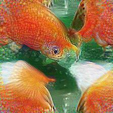
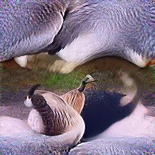
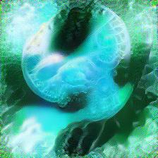
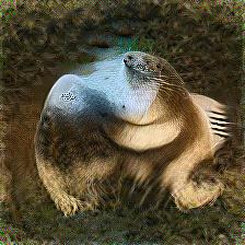
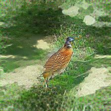
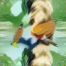
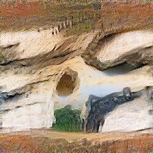
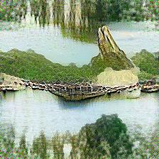
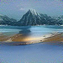
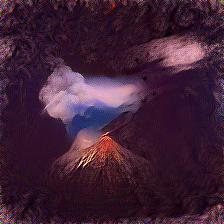
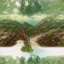
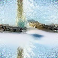
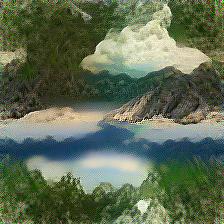
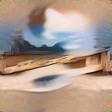
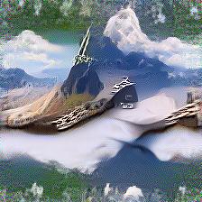
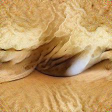
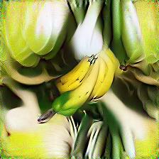
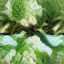
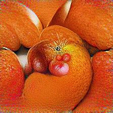
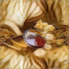
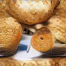
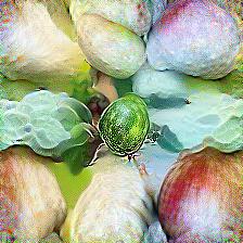
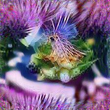
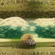
Cock Grey Owl Peacock Flamingo Gold Fish Goose Jellyfish Sea Lion Robin Bulbul Cliff Coral Reef Lakeside Seashore Volcano Valley Geyser Foreland Sandbar Alp Dough Banana Broccoli Orange Potato Bagel Fig cardoon Hay Strawberry

Figure 7: Visualizations of our synthetic images from ImageNet

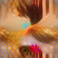
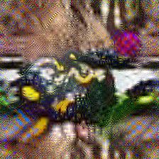
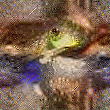
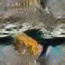
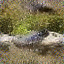
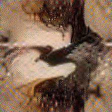
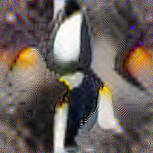
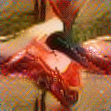
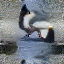
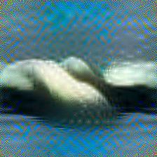
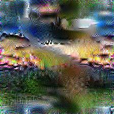
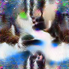
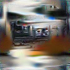
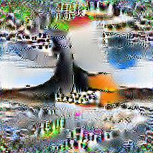
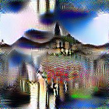
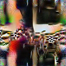
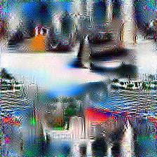
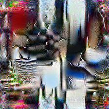
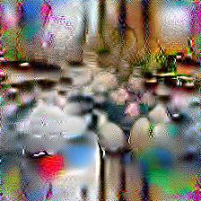
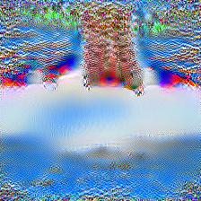
Goldfish Salamander Bullfrog TailedFrog Alligator Scorpion Penguin Lobster Sea Gull Sea Lion Tiny-ImageNet Tench Springer CassettePlyr Chain Saw Church FrenchHorn Garb. Truck Gas Pump Golf Ball Parachute ImageNette

Figure 8: Visualizations of our synthetic images on smaller datasets

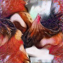
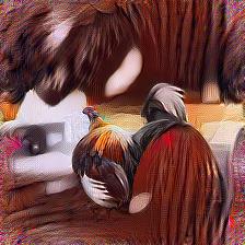
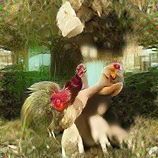
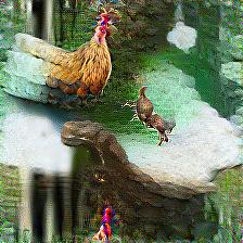
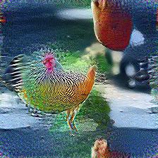
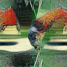
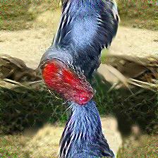
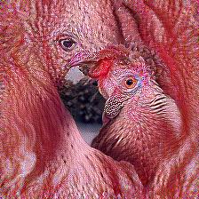
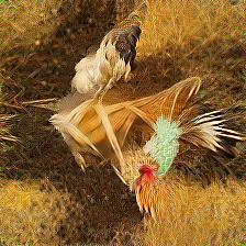
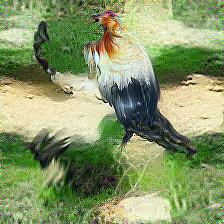
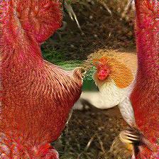
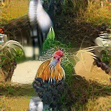
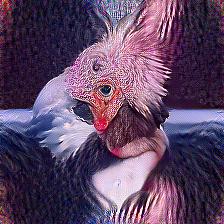
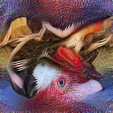
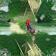
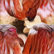
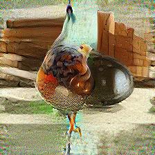
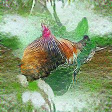
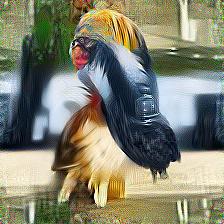
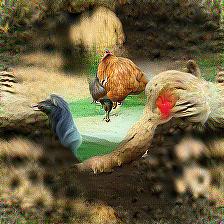
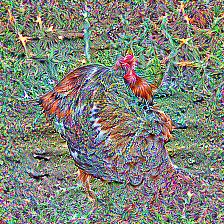
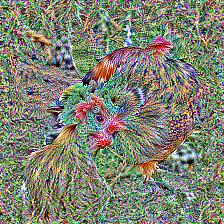
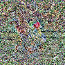
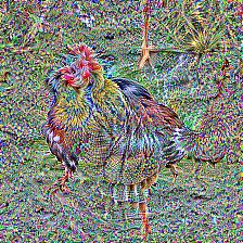
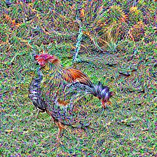
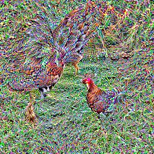
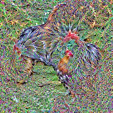
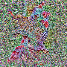
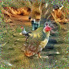
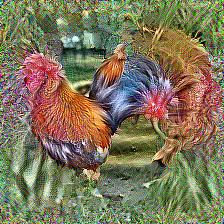
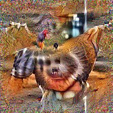
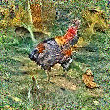
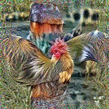
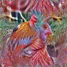
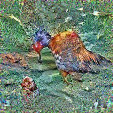
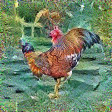
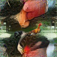
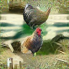
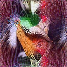
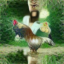
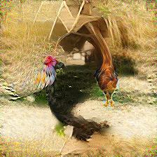
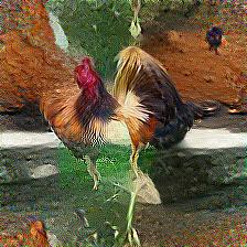
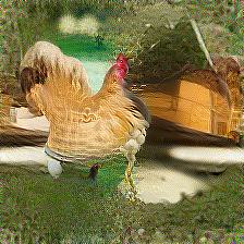
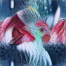
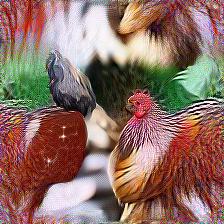
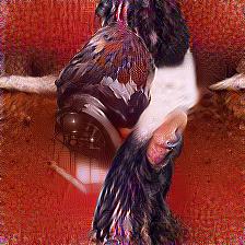
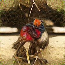
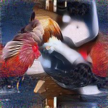
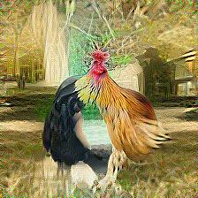
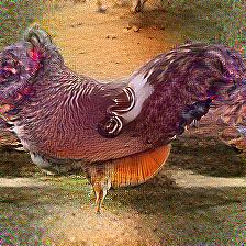
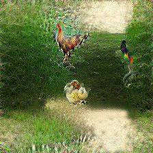
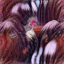
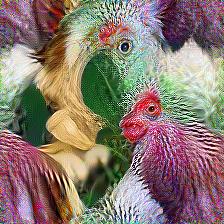
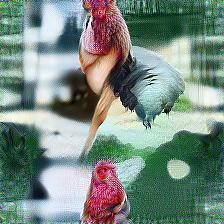
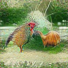
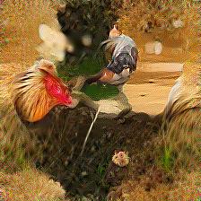
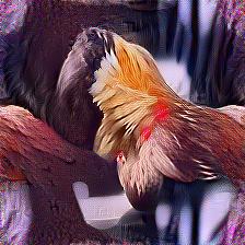
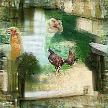
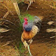
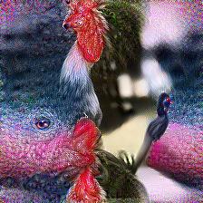
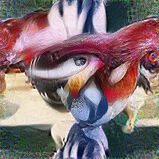
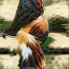
Barycenter Loss: Yes Barycenter Loss: No $\lambda=0.1$ $\lambda=1$ $\lambda=10$ $\lambda=100$ $\lambda=1000$

Figure 9: Visualization of synthetic images in ImageNet-1k with different regularization coefficient $\lambda$

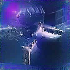
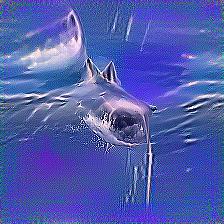
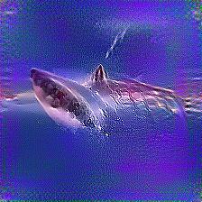
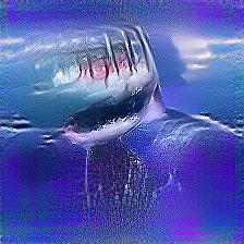
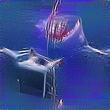
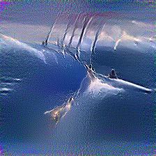
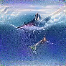
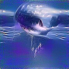
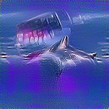
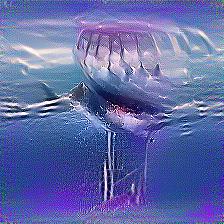
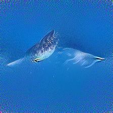
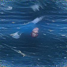
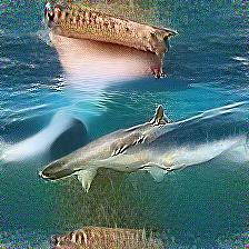
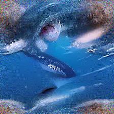
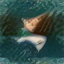
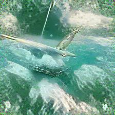
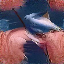
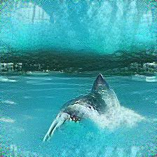
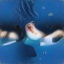
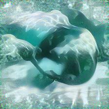
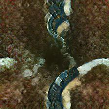
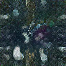
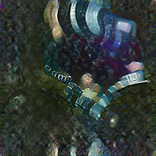
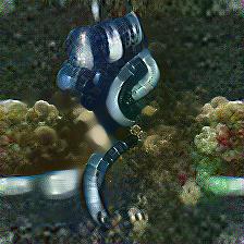
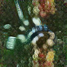
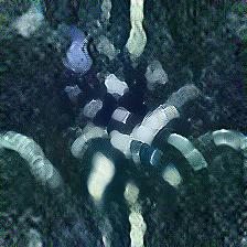
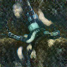
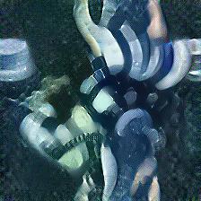
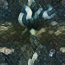
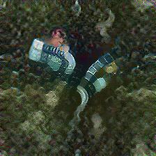
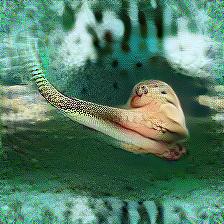
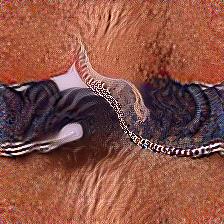
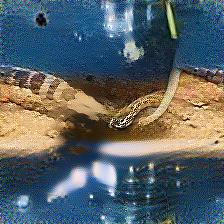
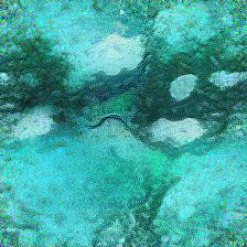
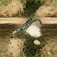
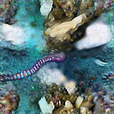
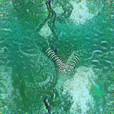
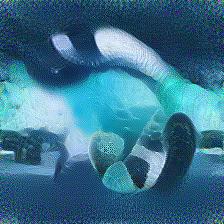
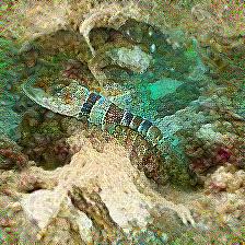
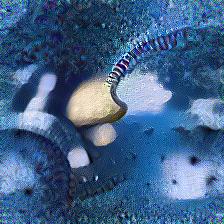
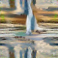
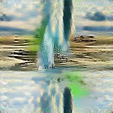
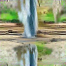
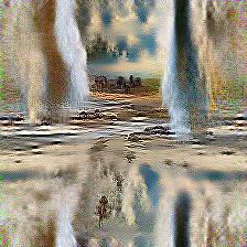
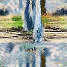
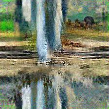
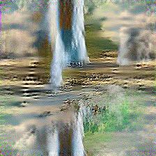
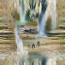
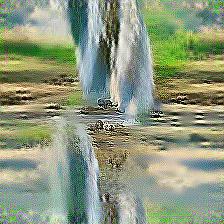
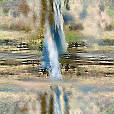
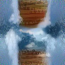
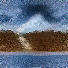
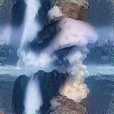
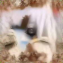
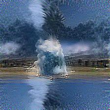
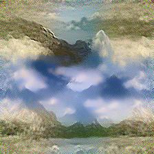
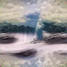
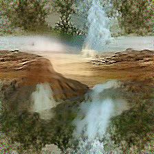
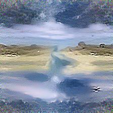
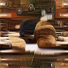
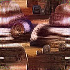
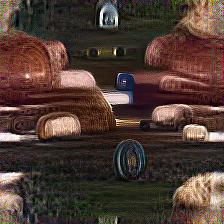
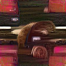
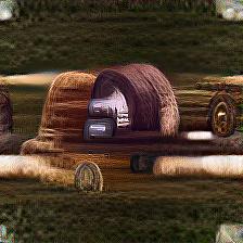
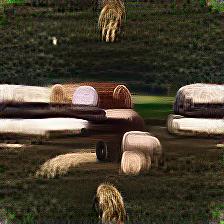
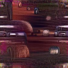
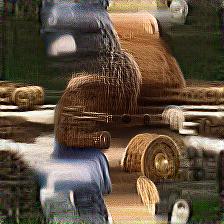
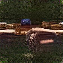
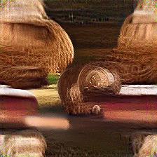
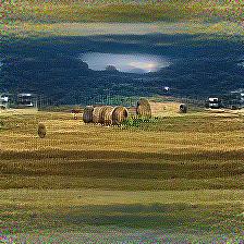
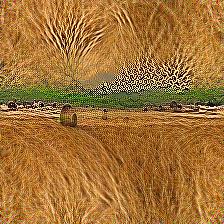
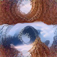
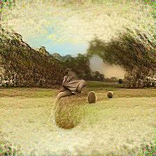
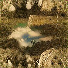
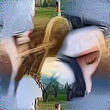
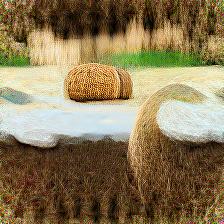
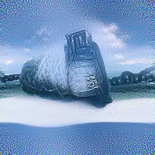
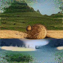
SRe²L synthetic images of class White Shark (classId: 002) Our synthetic images of the class White Shark (classId: 002) SRe²L synthetic images of class Sea Snake (classId: 065) Our synthetic images of the class Sea Snake (classId: 065) SRe²L synthetic images of class Geyser (classId: 974) Our synthetic images of the class Geyser (classId: 974) SRe²L synthetic images of class Hay (classId: 958) Our synthetic images of the class Hay (classId: 958)

Figure 10: Comparison of synthetic images obtained from our method vs. SRe²L on ImageNet-1k in 10 IPC setting. Our method yields synthetic images that better cover the diversity of real images within each class.

References

- [1] Tongzhou Wang, Jun-Yan Zhu, Antonio Torralba, and Alexei A Efros. Dataset distillation. arXiv preprint arXiv:1811.10959, 2018.
- [2] Bo Zhao, Konda Reddy Mopuri, and Hakan Bilen. Dataset condensation with gradient matching. In International Conference on Learning Representations, 2021.
- [3] Jie Zhang, Chen Chen, Bo Li, Lingjuan Lyu, Shuang Wu, Shouhong Ding, Chunhua Shen, and Chao Wu. DENSE: Data-free one-shot federated learning. In Alice H. Oh, Alekh Agarwal, Danielle Belgrave, and Kyunghyun Cho, editors, Advances in Neural Information Processing Systems, 2022.
- [4] Jack Goetz and Ambuj Tewari. Federated learning via synthetic data. arXiv preprint arXiv:2008.04489, 2020.
- [5] Felipe Petroski Such, Aditya Rawal, Joel Lehman, Kenneth Stanley, and Jeffrey Clune. Generative teaching networks: Accelerating neural architecture search by learning to generate synthetic training data. In International Conference on Machine Learning, pages 9206–9216. PMLR, 2020.
- [6] Noveen Sachdeva and Julian McAuley. Data distillation: A survey, 2023.
- [7] Bo Zhao and Hakan Bilen. Dataset condensation with differentiable siamese augmentation. In International Conference on Machine Learning, 2021.
- [8] George Cazenavette, Tongzhou Wang, Antonio Torralba, Alexei A. Efros, and Jun-Yan Zhu. Dataset distillation by matching training trajectories. In Proceedings of the IEEE/CVF Conference on Computer Vision and Pattern Recognition, 2022.
- [9] Seungjae Shin, Heesun Bae, Donghyeok Shin, Weonyoung Joo, and Il-Chul Moon. Loss-curvature matching for dataset selection and condensation, 2023.
- [10] Tongzhou Wang, Jun-Yan Zhu, Antonio Torralba, and Alexei A. Efros. Dataset distillation. arXiv preprint arXiv:2006.08545, 2020.
- [11] Noel Loo, Ramin Hasani, Alexander Amini, and Daniela Rus. Efficient dataset distillation using random feature approximation. In Alice H. Oh, Alekh Agarwal, Danielle Belgrave, and Kyunghyun Cho, editors, Advances in Neural Information Processing Systems, 2022.
- [12] Timothy Nguyen, Zhourong Chen, and Jaehoon Lee. Dataset meta-learning from kernel ridge-regression. In International Conference on Learning Representations, 2021.
- [13] Bo Zhao and Hakan Bilen. Dataset condensation with distribution matching. In Proceedings of the IEEE/CVF Winter Conference on Applications of Computer Vision, pages 6514–6523, 2023.
- [14] Kai Wang, Bo Zhao, Xiangyu Peng, Zheng Zhu, Shuo Yang, Shuo Wang, Guan Huang, Hakan Bilen, Xinchao Wang, and Yang You. Cafe: Learning to condense dataset by aligning features. In Proceedings of the IEEE/CVF Conference on Computer Vision and Pattern Recognition, pages 12196–12205, 2022.
- [15] Arthur Gretton, Karsten M Borgwardt, Malte J Rasch, Bernhard Schölkopf, and Alexander Smola. A kernel two-sample test. The Journal of Machine Learning Research, 13(1):723–773, 2012.
- [16] Ilya O Tolstikhin, Bharath K. Sriperumbudur, and Bernhard Schölkopf. Minimax estimation of maximum mean discrepancy with radial kernels. In D. Lee, M. Sugiyama, U. Luxburg, I. Guyon, and R. Garnett, editors, Advances in Neural Information Processing Systems, volume 29. Curran Associates, Inc., 2016.
- [17] Cédric Villani. Optimal Transport: Old and New, volume 338. Springer Science & Business Media, 2008.
- [18] Martial Agueh and Guillaume Carlier. Barycenters in the wasserstein space. SIAM Journal on Mathematical Analysis, 43(2):904–924, 2011.
- [19] Zeyuan Yin, Eric Xing, and Zhiqiang Shen. Squeeze, recover and relabel: Dataset condensation at imagenet scale from a new perspective, 2023.
- [20] Sergey Ioffe and Christian Szegedy. Batch normalization: Accelerating deep network training by reducing internal covariate shift. In International Conference on Machine Learning, pages 448–456. PMLR, 2015.
- [21] Marco Cuturi and Arnaud Doucet. Fast computation of wasserstein barycenters. In International conference on machine learning, pages 685–693. PMLR, 2014.
- [22] Jia Deng, Wei Dong, Richard Socher, Li-Jia Li, Kai Li, and Li Fei-Fei. Imagenet: A large-scale hierarchical image database. In 2009 IEEE conference on computer vision and pattern recognition, pages 248–255. Ieee, 2009.
- [23] Tongzhou Wang, Jun-Yan Zhu, Antonio Torralba, and Alexei A. Efros. Dataset distillation. arXiv preprint arXiv:1811.10959, 2018.
- [24] Ruonan Yu, Songhua Liu, and Xinchao Wang. Dataset distillation: A comprehensive review, 2023.
- [25] Yongchao Zhou, Ehsan Nezhadarya, and Jimmy Ba. Dataset distillation using neural feature regression. arXiv preprint arXiv:2206.00719v2, 2022.
- [26] Zhiwei Deng and Olga Russakovsky. Remember the past: Distilling datasets into addressable memories for neural networks. Advances in Neural Information Processing Systems, 35:34391–34404, 2022.
- [27] Songhua Liu, Kai Wang, Xingyi Yang, Jingwen Ye, and Xinchao Wang. Dataset distillation via factorization. Advances in Neural Information Processing Systems, 35:1100–1113, 2022.
- [28] Jiawei Du, Yidi Jiang, Vincent YF Tan, Joey Tianyi Zhou, and Haizhou Li. Minimizing the accumulated trajectory error to improve dataset distillation. In Proceedings of the IEEE/CVF Conference on Computer Vision and Pattern Recognition, pages 3749–3758, 2023.
- [29] Justin Cui, Ruochen Wang, Si Si, and Cho-Jui Hsieh. Scaling up dataset distillation to imagenet-1k with constant memory. In International Conference on Machine Learning, pages 6565–6590. PMLR, 2023.
- [30] Bo Zhao and Hakan Bilen. Synthesizing informative training samples with gan. arXiv preprint arXiv:2204.07513, 2022.
- [31] Hae Beom Lee, Dong Bok Lee, and Sung Ju Hwang. Dataset condensation with latent space knowledge factorization and sharing. arXiv preprint arXiv:2208.10494, 2022.
- [32] Zhiqiang Shen and Eric Xing. A fast knowledge distillation framework for visual recognition. In Computer Vision–ECCV 2022: 17th European Conference, Tel Aviv, Israel, October 23–27, 2022, Proceedings, Part XXIV, pages 673–690. Springer, 2022.
- [33] Jules Vidal, Joseph Budin, and Julien Tierny. Progressive wasserstein barycenters of persistence diagrams. IEEE Transactions on Visualization and Computer Graphics, page 1–1, 2019.
- [34] Lei Yang, Jia Li, Defeng Sun, and Kim-Chuan Toh. A fast globally linearly convergent algorithm for the computation of wasserstein barycenters, 2020.
- [35] Steffen Borgwardt and Stephan Patterson. On the computational complexity of finding a sparse wasserstein barycenter, 2022.
- [36] Jiaojiao Fan, Amirhossein Taghvaei, and Yongxin Chen. Scalable computations of wasserstein barycenter via input convex neural networks, 2021.
- [37] Florian Heinemann, Axel Munk, and Yoav Zemel. Randomised wasserstein barycenter computation: Resampling with statistical guarantees, 2021.
- [38] Ahmad Sajedi, Samir Khaki, Ehsan Amjadian, Lucy Z Liu, Yuri A Lawryshyn, and Konstantinos N Plataniotis. Datadam: Efficient dataset distillation with attention matching. In Proceedings of the IEEE/CVF International Conference on Computer Vision, pages 17096–17107, 2022.
- [39] Hongxu Yin, Pavlo Molchanov, Jose M Alvarez, Zhizhong Li, Arun Mallya, Derek Hoiem, Niraj K Jha, and Jan Kautz. Dreaming to distill: Data-free knowledge transfer via deepinversion. In Proceedings of the IEEE/CVF Conference on Computer Vision and Pattern Recognition, pages 8715–8724, 2020.
- [40] Kaiming He, Xiangyu Zhang, Shaoqing Ren, and Jian Sun. Deep residual learning for image recognition. In Proceedings of the IEEE conference on computer vision and pattern recognition, pages 770–778, 2016.
- [41] Rémi Flamary, Nicolas Courty, Alexandre Gramfort, Mokhtar Z. Alaya, Aurélie Boisbunon, Stanislas Chambon, Laetitia Chapel, Adrien Corenflos, Kilian Fatras, Nemo Fournier, Léo Gautheron, Nathalie T.H. Gayraud, Hicham Janati, Alain Rakotomamonjy, Ievgen Redko, Antoine Rolet, Antony Schutz, Vivien Seguy, Danica J. Sutherland, Romain Tavenard, Alexander Tong, and Titouan Vayer. Pot: Python optimal transport. Journal of Machine Learning Research, 22(78):1–8, 2021.
- [42] George Cazenavette, Tongzhou Wang, Antonio Torralba, Alexei A. Efros, and Jun-Yan Zhu. Generalizing dataset distillation via deep generative prior. CVPR, 2023.
- [43] Shiye Lei and Dacheng Tao. A comprehensive survey of dataset distillation. arXiv preprint arXiv:2301.05603, 2022.
- [44] Alexey Dosovitskiy, Lucas Beyer, Alexander Kolesnikov, Dirk Weissenborn, Xiaohua Zhai, Thomas Unterthiner, Mostafa Dehghani, Matthias Minderer, Georg Heigold, Sylvain Gelly, et al. An image is worth 16x16 words: Transformers for image recognition at scale. arXiv preprint arXiv:2010.11929, 2020.
- [45] Laurens Van der Maaten and Geoffrey Hinton. Visualizing data using t-sne. Journal of machine learning research, 9(11), 2008.
- [46] Yu Nesterov. Smooth minimization of non-smooth functions. Mathematical programming, 103:127–152, 2005.
- [47] Amir Beck and Marc Teboulle. Mirror descent and nonlinear projected subgradient methods for convex optimization. Operations Research Letters, 31(3):167–175, 2003.
- [48] TorchVision maintainers and contributors. Torchvision: Pytorch’s computer vision library. https://github.com/pytorch/vision, 2016.