Perturbation-based Analysis of Compositional Data

Abstract

Existing statistical methods for compositional data analysis are inadequate for many modern applications for two reasons. First, modern compositional datasets, for example in microbiome research, display traits such as high-dimensionality and sparsity that are poorly modelled with traditional approaches. Second, assessing – in an unbiased way – how summary statistics of a composition (e.g., racial diversity) affect a response variable is not straightforward. In this work, we propose a framework based on hypothetical data perturbations that addresses both issues. Unlike existing methods for compositional data, we do not transform the data and instead use perturbations to define interpretable statistical functionals on the compositions themselves, which we call average perturbation effects. These average perturbation effects, which can be employed in many applications, naturally account for confounding that biases frequently used marginal dependence analyses. We show how average perturbation effects can be estimated efficiently by deriving a perturbation-dependent reparametrization and applying semiparametric estimation techniques. We analyze the proposed estimators empirically on simulated data and demonstrate advantages over existing techniques on US census and microbiome data. For all proposed estimators, we provide confidence intervals with uniform asymptotic coverage guarantees.

Keywords: compositional data, causality, perturbation, feature importance, diversity effects, nonparametrics

1 Introduction

Compositional data, that is, measurements consisting of parts of a whole, appear in many scientific disciplines, for example, rock compositions in geology, green house gases in the atmosphere, species compositions in ecology and racial or gender distributions in social sciences. The defining property of such data is that they only capture information relative to the unknown whole and hence do not contain any information on the absolute sizes. Depending on the application, the absolute information either might not be of interest (e.g., when analyzing racial or gender distributions) or might not be easily accessible with existing measuring techniques (e.g., in ecology). Mathematically, a $d$-coordinate composition can – without loss of information – be normalized such that it is represented as a point on the $(d-1)$-dimensional simplex

$$\Delta^{d-1}:=\left\{z=(z^{1},\dots,z^{d})\in[0,1]^{d}\mid\textstyle\sum_{j=1}^{d}z^{j}=1\right\}.$$

It is well-known that many conventional statistical procedures become invalid when applied to compositional data. For example, already Pearson (1897) drew attention to the fact that correlations between individual compositional components can be spurious due to the sum-to-one constraint. Much work has gone into constructing new procedures for adjusting the correlation measure for compositional components, e.g., by transforming the data with log-ratio transforms (Aitchison, 1982). An instructive viewpoint is to see these approaches not as adjusting the correlation measure but rather as creating new target parameters (e.g., the correlation between log-ratios) that have meaningful interpretations in compositional data.

We adopt this point of view and develop a framework which uses hypothetical perturbations of the data to construct meaningful target parameters. Specifically, we consider a setting where we observe an outcome of interest $Y\in\mathbb{R}$ and an associated compositional predictor $Z\in\Delta^{d-1}$. Our goal is to construct functionals of the conditional distribution $Y$ given $Z$ that are useful when analyzing compositional data. To illustrate this, we consider two examples in which existing approaches are insufficient.

Example 1 (Effects of presence or absence of microbes).

Consider the problem of determining whether the presence or absence of certain microbes in the human gut is affecting a disease. Microbial abundances are commonly measured using genetic sequencing (e.g., targeted amplicon or shotgun metagenomic sequencing) which in most cases only measures the composition and not the absolute abundances. Assume we have measurements from a cohort of patients, where for each patient the relative abundance of all microbes in their gut $Z\in\Delta^{d-1}$ and a disease indicator $Y\in\{0,1\}$ has been recorded. While estimating causal effects in such a setting is often too ambitious, one could hope to screen for relevant microbes that could then be considered for follow-up randomized studies. One possible approach (e.g., Hu et al., 2021) would be to consider a fixed microbe $j$ and then compare the distributions

$$Y\,|\,Z^{j}=0\quad\text{and}\quad Y\,|\,Z^{j}\neq 0$$

for example, with an independence test or by regressing $Y$ on $\mathbbm{1}_{\{Z^{j}=0\}}$. It is well-known that this type of marginal dependence analysis can be misleading if dependencies exist between the individual components. As an example, assume the disease indicator is generated by

$$Y\sim\operatorname{Ber}(\tfrac{3}{4}+\tfrac{1}{8}\mathds{1}_{\{Z^{1}=0\}}-\tfrac{1}{2}\mathds{1}_{\{Z^{2}=0\}}),$$

that is, the absence of $Z^{1}$ increases while the absence of $Z^{2}$ decreases the probability of having the disease. In a numerical simulation of this generative model with dependence between $Z^{1}$ and $Z^{2}$, the effect of $Z^{1}$ is instead estimated to decrease the probability of disease as shown in Table 1. If $Z$ did not live on the simplex, we could adjust for the dependence in the remaining coordinates by considering conditional dependencies of the form $Y\mbox{${}\perp\mkern-11.0mu\perp{}$}Z^{j}\,|\,Z^{-j}$. However, due to the simplex constraint $Z^{-j}$ completely determines $Z^{j}$, so the conditional independence always holds. In the Table 1, we also provide the results from applying the compositional knockout effect to $Z^{1}$ $(\mathrm{CKE}^{1})$ which we introduce in Section 2.2.

Example 1
method	estimate	95%-CI
OLS of $Y$ on $\mathbbm{1}_{\{Z^{1}=0\}}$	$-0.12$	$(-0.17,-0.06)$
$\mathrm{CKE}^{1}$ using rf	$0.15$	$(0.10,0.21)$

Example 2
method	estimate	95%-CI
OLS of Y on $-G(Z)$	$-1.57$	$(-2.18,-0.97)$
$\mathrm{CDI}_{\mathrm{Gini}}$ using rf	$0.63$	$(0.14,1.12)$

Table 1: Numerical illustration of Examples 1 and 2. The first row in each table corresponds to the marginal effect estimate based on a correctly specified linear model. The second row correspond to estimates of two of the target parameters introduced in Section 2.2 with random forest (rf) as nuisance function estimators. (Left) The estimated marginal effect is negative, even though the true effect is positive. The compositional knock-out effect ($\mathrm{CKE}^{1}$), which adjust for the simplex structure, results in the correct sign. (Right) The estimated marginal effect of an increase in diversity (measured by the negative Gini coefficient, i.e., $-G(Z)$) is negative even though the true effect is equal to $1$ by construction. The compositional diversity effect $\mathrm{CDI}_{\mathrm{Gini}}$ correctly recovers the effect. Details on both experiments are provided in Section S4.1 of the supplementary material.

Example 2 (Effects of increased diversity).

Consider the problem of determining the effect of an increase in diversity of $Z$ on the response $Y$. Such a question is of immediate interest in many applied fields, e.g. when investigating whether more racially diverse university programs improve educational outcomes (Antonio et al., 2004) or whether increased income equality boosts economic output (Shin, 2012). The prevalent approach is to summarize diversity via a one-dimensional summary statistic $G(Z)$ (e.g., the Gini coefficient, generalized entropy or Gini-Simpson index) and analyze the correlation between $G(Z)$ and $Y$. As in Example 1 this type of marginal dependence analysis is potentially misleading in practice. In Table 1 we illustrate this on a specific numeric example, where the true causal effect is positive, but the marginal method leads to a negative effect of diversity (details are provided in Section S4.1 of the supplementary material). To avoid this, one would again like to adjust for the remaining dependence within $Z$ to avoid the confounding biases. However, since $G(Z)$ depends on all of $Z$ existing adjustment approaches are not applicable. The compositional diversity effect (with Gini-speed) which we introduce in Section 2.2 appropriately adjust for the confounding as shown in Table 1. A more in-depth example in which the marginal approach is misleading is given in Section 4.2 where we estimate the effect of racial diversity on income on grouped real data. Unlike in Example 1, the problem of not being able to adjust with existing techniques is not solely due to the simplex-constraint and similarly appears for summary statistics of unconstrained Euclidean data. Our perturbation-based framework can also be extended to those settings, but as the use of this type of analysis is particularly prevalent in compositional data applications we restrict our attention to this setting.

In this work, we propose a procedure that accounts for potential confounding within $Z$. The main idea is to introduce a new target parameter via a hypothetical perturbation of the data. More concretely, a perturbation is a function $\psi:\mathcal{D}\subseteq\Delta^{d-1}\times[0,\infty)\rightarrow\Delta^{d-1}$ which for each point $z\in\Delta^{d-1}$ describes a path $\gamma\mapsto\psi(z,\gamma)$ along which the point $z$ should be changed. For example, in Example 1 when considering the first microbe (i.e., $j=1$), we could consider a binary perturbation $\psi$ satisfying for all $z\in\Delta^{d-1}$ that $\psi(z,0)=z$ and $\psi(z,1)=(0,\mathsf{C}(z^{-j}))$, where $\mathsf{C}(\cdot)$ scales the inputs to have sum one. A target parameter that captures the desired adjusted effect is then given by

$$\lambda_{\psi}:=\frac{\mathbb{E}\left[\mathbb{E}[Y\,|\,Z=\psi(Z,1)]\right]-\mathbb{E}\left[\mathbb{E}[Y\,|\,Z=\psi(Z,0)]\right]}{\mathbb{P}(Z\neq\psi(Z,1))}.$$

In Example 2, an increase in the diversity of $Z$ can be expressed as a perturbation $\psi$ that pushes every point in $\Delta^{d-1}$ to a more diverse point. Formally, using the center of the simplex (i.e., $z_{\mathrm{cen}}=(1/d,\ldots,1/d)\in\Delta^{d-1}$) as the most diverse point, we define for all $z\in\Delta^{d-1}$ and all $\gamma\in[0,\|z_{\mathrm{cen}}-z\|_{1}]$ the perturbation

$$\psi(z,\gamma)=z+\gamma\frac{z_{\mathrm{cen}}-z}{\|z_{\mathrm{cen}}-z\|_{1}}.$$

We can then interpret $\psi(z,\epsilon)$ for a small $\epsilon>0$ as slightly increasing the diversity of the point $z$. With this notion of an increase in diversity, a target parameter that captures the desired adjusted effect is given by

$$\tau_{\psi}:=\mathbb{E}\left[\partial_{\gamma}\mathbb{E}\left[Y\,|\,Z=\psi(Z,\gamma)\right]\big{|}_{\gamma=0}\right],$$

which quantifies how on average the conditional expectation of $Y$ given $Z$ is affected by small increases in diversity. A key strength of using perturbations to define target parameters is that it makes them easy to communicate, interpret and discuss with practitioners. From our experience, practitioners often have a good understanding of what perturbation they are interested in and formalizing them mathematically as above is straight-forward. Even though the target parameters $\lambda_{\psi}$ and $\tau_{\psi}$ have a clear causal motivation, it is important to stress that they are purely (observational) statistical quantities. To connect them to causal effects requires standard causal assumptions and potentially adjustments to the estimators, which we discuss in Section 2.3.

While the target parameters $\lambda_{\psi}$ and $\tau_{\psi}$ may seem simple at first sight, they can be challenging to estimate directly as they depend on estimating the conditional expectation $z\mapsto\mathbb{E}[Y\,|\,Z=z]$ which due the simplex structure is generally a complex functional. We therefore propose an approach that reparametrizes the compositional vector $Z\in\Delta^{d-1}$ via a bijection $\phi$ to a vector $(L,W)\in\mathbb{R}\times\mathcal{W}$ in such a way that the perturbation only changes $L$ in the new parametrization. To make this more concrete, assume that the structural causal model (SCM) (e.g., Pearl, 2009) given in Figure 1 (left) generates the data (the causal terminology is used only to provide a more intuitive introduction). Given a perturbation $\psi$ that we are interested in, we now propose to construct a bijection $\phi:\Delta^{d-1}\rightarrow\mathbb{R}\times\mathcal{W}$ that maps $Z$ to $(L,W)$ such that if we intervene on $Z$ by setting it to $\psi(Z,\gamma)$ this corresponds to an intervention in an SCM over the variables $(Y,L,W)$ on $L$ alone (see Figure 1 (right)). Hence, if we are able to construct such a reparametrization, then we have successfully reduced our problem to a setting in which standard adjustment works, that is, using any existing method to estimate the effect of $L$ on $Y$ that adjusts for $W$ results in an unbiased estimate of the causal effect. Given a perturbation $\psi$, we provide a general recipe to construct the reparametrization $\phi$. We furthermore propose several explicit perturbations (including their corresponding reparametrizations) and suggest efficient estimators of the perturbation-based target parameters using semiparametric theory based on the $(L,W)$-reparametrization.

(a) SCM on $Z$-scale (b) SCM on $(L,W)$-scale

$$Y \leftarrow f(Z,\eta)$$

$$L \leftarrow m(W,\xi)$$

$$Y \leftarrow h(L,W,\varepsilon)$$

Figure 1: (a) Data-generating SCM on the $Z$-scale. $Z\in\Delta^{d-1}$ is a compositional vector, $Y$ is a response variable and $\eta$ is exogenous noise. (b) Reparametrized SCM on the $(L,W)$-scale. $(L,W)=\phi(Z)$ are the reparametrized predictors, $Y$ is the same response as in (a) and $\xi$ and $\varepsilon$ are exogenous noise variables. The reparametrization needs to disentangle the perturbation effect on $Z$ in a way such that intervening on $Z$ by setting it to $\psi(Z,\gamma)$ corresponds to intervening on only $L$ (red double head arrows).

The remainder of the paper is structured as follows. In Section 1.1 we discuss existing methods for compositional data analysis and how our approach contributes to this research. Section 1.2 collects the mathematical notation used throughout this work. Our perturbation-based framework is introduced in Section 2. In Section 2.1, we provide a way to construct interpretable perturbations based on suitably choosing the endpoint, direction and speed of the perturbation. We also provide a general construction for the aforementioned $L$ and $W$ for a wide range of perturbations. We end the section by discussing how to adapt our proposals to general geometries on the simplex including those employed by many current methods in compositional data analysis. In Section 2.2 we highlight and name some of the perturbation effects that we believe are most useful for practitioners and provide some examples of how and when these effects should be applied. In Section 3, we discuss how to estimate the parameters of interest based on semiparametric theory using two different methods that represent a trade-off between generality and robustness. Our semiparametric estimators and perturbation effects are then illustrated on both simulated data and two real-world applications in Section 4. Finally, we present the theoretical guarantees of our estimates in Section 5.

1.1 Relation to existing compositional data analysis approaches

Compositional data analysis has a long history dating back to Pearson (1897). The most prevalent class of methods is based on the seminal paper by Aitchison (1982) which introduces the log-ratio approach. In its most basic form it consists of transforming the simplex data via the additive, centered or isometric log-ratio transforms (Aitchison, 1982; Egozcue et al., 2003) and then performing the statistical analysis in the transformed space. By considering ratios instead of compositional coordinates it avoids the common pitfalls of spurious correlations that occur by comparing coordinates. Our approach is not based on log-ratios, but it is possible to construct perturbations from this perspective (see Section 2.1.3). Furthermore, some of the perturbation effects that we highlight as interpretable overlap with effects that can also be deduced from the log-ratio perspective. Most prominently, we consider a class of compositional feature influence measures for which a certain member (multiplicative speed, see Example 3) corresponds to the compositional feature influence which has been previously proposed by Huang et al. (2023). It also corresponds to one of the coefficients in a log-contrast model (Aitchison and Bacon-Shone, 1984) if the conditional mean lies in the log-contrast model class. Our perturbation-based framework, however, has a fundamentally different starting point and allows for the construction of perturbations that are not related to the log-ratio approach.

The idea of transforming compositional data via the log-ratio transform to a simpler sample space has been applied successfully in many applications, however we believe its indirect use of the data is restrictive. This is best illustrated by the so-called zero-problem that occurs because the log-ratio approach, in general, cannot be applied in settings with too many zeros. This problem has sparked a large body of research developing various types of zero-imputation schemes (e.g., Martín-Fernández et al., 2000, 2003, 2015; Palarea-Albaladejo and Martín-Fernández, 2008; Lubbe et al., 2021) that can be used before applying the log-ratio approach. Other approaches advocate the use of different transformations, for example power-transformations (Greenacre, 2009) or spherical transformations (Scealy and Welsh, 2011; Li and Ahn, 2022). While many of these approaches are sensible in specific applications, we believe that it is generally preferable to modify the statistical procedure to fit the data rather than vice versa. Greenacre et al. (2023) provide an overview of current state-of-the-art compositional data analysis and highlights some of the shortcomings in existing transformation-based approaches. In contrast to these methods, our perturbation-based framework works directly with the compositional data and defines the target parameter from this perspective. In the presence of zeros, perturbations that directly incorporate or omit zeros can be selected based on the application. Furthermore, we can construct perturbation effects that directly capture the effect of setting certain components to zero.

1.2 Notation

We use superscripts to index coordinates of a vector throughout, that is, for $x\in\mathbb{R}^{d}$ we write $x^{j}$ for the $j$th coordinate of $x$ and denote by $e_{j}$ the $j$th canonical unit vector in $\mathbb{R}^{d}$. For all $n\in\mathbb{N}$, we define $[n]:=\{1,\dots,n\}$. For a real-valued function $f:\mathcal{X}\rightarrow\mathbb{R}$ with $\mathcal{X}\subseteq\mathbb{R}^{d}$, we denote by $\partial_{x^{j}}$ the partial derivative of $f$ with respect to the $x^{j}$ coordinate and the gradient (vector of partial derivatives) of $f$ is denoted by $\nabla f$. When differentiating a function of a single variable at a boundary point of the domain, we only consider the one-sided limit. For $p\geq 1$ and $x\in\mathbb{R}^{d}$, we define $\|x\|_{p}:=\left(\sum_{j=1}^{d}\left|x^{j}\right|^{p}\right)^{1/p}$. Lastly, we define $\mathsf{C}(z):=z/\sum_{j=1}^{d}z^{j}$, the (simplex) closure operator, with the additional convention that for $0\in\mathbb{R}^{d}$ we have $\mathsf{C}(0)=(1/d,\dots,1/d)=:z_{\mathrm{cen}}$.

2 Target parameters via perturbations

For a response $Y\in\mathbb{R}$ and a compositional predictor $Z\in\mathcal{Z}\subseteq\Delta^{d-1}$, we seek to summarize the effect of $Z$ on the expectation of $Y$ under a pre-specified change of $Z$. We specify this change via perturbations.

Definition 1 (perturbations).

Let $\mathcal{D}\subseteq\mathcal{Z}\times[0,\infty)$ be such that for all $z\in\mathcal{Z}$ it holds that $\{z\}\times\{0\}\in\mathcal{D}$. We call a function $\psi=(\psi^{1},\dots,\psi^{d}):\mathcal{D}\to\Delta^{d-1}$ a perturbation if it satisfies for all $z\in\mathcal{Z}$ that $\psi(z,0)=z$. For all $z\in\mathcal{Z}$ we define the $\gamma$-domain and endpoint of $\psi$ (if it exists) by

$$\mathcal{I}_{\psi}(z):=\{\gamma\in[0,\infty)\mid(z,\gamma)\in\mathcal{D}\}\quad\text{and}\quad E_{\psi}(z):=\lim_{\gamma\to\sup\mathcal{I}_{\psi}(z)}\psi(z,\gamma),$$

respectively. We furthermore say that

1. $\psi$ is a binary perturbation if for all $z\in\mathcal{Z}$ it holds that $\mathcal{I}_{\psi}(z)=\{0,1\}$, i.e. $\mathcal{D}=\mathcal{Z}\times\{0,1\}$, and

2. $\psi$ is a directional perturbation if for all $z\in\mathcal{Z}$ there exists $\epsilon>0$ with $[0,\epsilon)\subseteq\mathcal{I}_{\psi}(z)$ and $\omega_{\psi}(z):=\partial_{\gamma}\psi(z,\gamma)\big{|}_{\gamma=0}$ exists. We further define the direction and speed of the perturbation for all $z\in\mathcal{Z}$ by

   $$v_{\psi}(z):=\mathbbm{1}_{\{\omega_{\psi}(z)=0\}}\frac{\omega_{\psi}(z)}{\|\omega_{\psi}(z)\|_{1}}\quad\text{}\quad s_{\psi}(z):=\|\omega_{\psi}(z)\|_{1},$$

   respectively.

Binary perturbations describe discrete changes that move each point to a specific endpoint, that is, they capture the difference between $\gamma=0$ (doing nothing) and $\gamma=1$ (applying the perturbation). An example of this is setting the first component of $Z$ to $0$. Directional perturbations describe ‘local’ changes to $Z$, that is, differences in $\gamma=0$ (doing nothing) and $\gamma=\epsilon$ for some small $\epsilon>0$ (moving slightly along the perturbation path). We later focus on the derivative of the perturbation at $\gamma=0$ as this captures the rate of change of directional perturbations at the initial point. As we only intend to use this initial derivative, it suffices to consider perturbations of the form

$$\psi(z,\gamma)=z+\gamma s_{\psi}(z)v_{\psi}(z).$$ (1)

We will discuss how to construct perturbations with interpretable directions and speeds in Section 2.1.2. Choosing to have the direction and speed parametrized by the $1$-norm is an arbitrary choice that turns out to be convenient on the simplex. In this work, we only consider binary and directional perturbations but other classes of perturbations could be of interest too. Perturbations can also be defined on more general sample spaces than simplices and many of the perturbation-related concepts described here can be readily extended to these settings.

Using the two types of perturbations, we can define informative summary statistics that capture the effect of the perturbations on the response. We do this by using contrasts of the perturbation, similar to how causal effects are defined via contrasts of interventions in the causal inference literature. Formally, we define the following target parameters associated with each type of perturbation.

Definition 2 (average perturbation effects).

Let $\mathcal{Z}\subseteq\Delta^{d-1}$, let $(Y,Z)\in\mathbb{R}\times\mathcal{Z}$ be random variables and define $f:z\mapsto\mathbb{E}[Y\,|\,Z=z]$. Then, for a binary perturbation $\psi$, if $f$ is identified on $\{\psi(z^{\prime},1)\in\Delta^{d-1}\mid z^{\prime}\in\mathcal{Z}\}$ and $\mathbb{P}(Z\neq\psi(Z,1))>0$, we define the average (binary) perturbation effect by

$$\lambda_{\psi}:=\frac{\mathbb{E}\left[f(\psi(Z,1))\right]-\mathbb{E}\left[Y\right]}{\mathbb{P}(Z\neq\psi(Z,1))}.$$

Furthermore, for a directional perturbation $\psi$, if for all $z\in\mathcal{Z}$ it holds that $f$ is differentiable on the simplex(see Section S1 for a precise definition) at $z$, we define the average (directional) perturbation effect by

$$\tau_{\psi}:=\mathbb{E}\left[\partial_{\gamma}f(\psi(Z,\gamma))\big{|}_{\gamma=0}\right].$$

We showcase different potential applications for both types of perturbation effect in the numerical experiments in Section 4. For binary perturbations, the denominator is included to scale the effect by the probability that the perturbation does not change $Z$. This is not required but in many cases provides a more meaningful parameter if one is interested in how the perturbation affects points on the simplex that are not yet at their endpoint. While both target parameters have obvious similarities to causal effects, they are a priori only (observational) statistical quantities. In particular, they are identifiable from the observational distribution as long as the conditions in Definition 2 are satisfied. We discuss the assumptions required for causal conclusions in Section 2.3.

Direct estimation of both target parameters relies on estimating the regression function $f:z\mapsto\mathbb{E}[Y\mid Z=z]$ and taking averages (see Section 3). An alternative estimation procedure for the effect of a binary perturbation $\lambda_{\psi}$ can be derived from noting that, if $L=\mathbbm{1}_{\{Z=\psi(Z,1)\}}$ and $W=\psi(Z,1)$, then

$$\mathbb{E}[Y\,|\,L=1,W]=\frac{\mathbb{E}[YL\,|\,W]}{\mathbb{E}[L\,|\,W]}=f(W).$$

Therefore, we can write

$$\lambda_{\psi}=\frac{\mathbb{E}[\mathbb{E}[Y\,|\,L=1,W]-Y]}{\mathbb{P}(L=0)},$$ (2)

which is an expression more amenable to analysis by semiparametric theory and thus allows us to construct efficient estimators. If we are willing to assume that $f(\psi(Z,1))-f(Z)$ is constant when $L=0$ and equal to, say $\theta$, then

$$\lambda_{\psi}=\frac{\mathbb{E}[\{f(W)-f(Z)\}(1-L)]}{\mathbb{P}(L=0)}=\theta$$

and furthermore

$$\mathbb{E}[Y\,|\,Z]=f(Z)=f(W)L+(f(Z)-f(W)+f(W))(1-L)=\theta L+\underbrace{f(W)-\theta}_{h(W)},$$

so $\theta$ is the coefficient of $L$ in a partially linear model of $Y$ on $L$ and $W$.

It would be convenient to also phrase the average directional perturbation effect $\tau_{\psi}$ as a quantity that is similarly amenable to semiparametric analysis and permits us to impose a partially linear model. To motivate the upcoming condition, we consider what happens when $Z$ takes values in $\mathbb{R}^{d}$. In that case, we can write

$$\partial_{\gamma}f(\psi(z,\gamma))\big{|}_{\gamma=0}=\nabla f(z)^{\top}\omega_{\psi}(z).$$

We now want to isolate the change of $\psi$ in the direction $v_{\psi}$ into a real-valued variable $L$ while keeping the remainder of the ‘information’ in $Z$ in an additional variable $W$. For a reparametrization $\phi$ of $z$ into $(\ell,w)\in\mathbb{R}\times\mathcal{W}$, we define the reparametrized $f$ as $g:(\ell,w)\mapsto f(\phi^{-1}(\ell,w))$. Then, in order for the reparametrization $\phi$ to separate the ’information’ appropriately, we require

$$\partial_{\ell}g(\ell,w)=\partial_{\ell}f(\phi^{-1}(\ell,w))=\nabla f(\phi^{-1}(\ell,w))^{\top}\partial_{\ell}\phi^{-1}(\ell,w)$$

to equal $\partial_{\gamma}f(\psi(z,\gamma))\big{|}_{\gamma=0}$, that is,

$$\omega_{\psi}(\phi^{-1}(\ell,w))=\partial_{\ell}\phi^{-1}(\ell,w).$$

This derivation is only morally correct when $Z\in\Delta^{d-1}$ ($\nabla f$ is not defined in the usual sense for simplex-valued functions) and to make it formally correct one needs to apply techniques from differential geometry. The proof of the following result can be found in Section S2.1 of the supplementary material.

Proposition 1 (derivative-isolating).

Consider the setting of Definition 2. Let $\mathcal{W}$ be a set and $(\mathcal{L}_{w})_{w\in\mathcal{W}}$ a family of subsets of $\mathbb{R}$. Suppose that $\phi=(\phi^{L},\phi^{W}):\mathcal{Z}\to\{(\ell,w)\in\mathbb{R}\times\mathcal{W}\mid w\in\mathcal{W},\ell\in\mathcal{L}_{w}\}$ is a bijection and $\psi$ a directional perturbation such that for all $z\in\mathcal{Z}$ it holds that $\omega_{\psi}(z)\neq 0$. Suppose that for all $w\in\mathcal{W}$ and all $\ell\in\mathcal{L}_{w}$, we have

$$\omega_{\psi}(\phi^{-1}(\ell,w))=\partial_{\ell}\phi^{-1}(\ell,w).$$ (3)

Then, defining $g:(\ell,w)\mapsto f(\phi^{-1}(\ell,w))$ and $(L,W)=\phi(Z)$, the average perturbation effect satisfies

$$\tau_{\psi}=\mathbb{E}\left[\partial_{\ell}g(\ell,W)\bigm{|}_{\ell=L}\right].$$ (4)

We say that $\phi$ is derivative-isolating if it satisfies (3).

From this result it follows that if we are able to find a derivative-isolating reparametrization (we describe how to find such reparametrizations for certain perturbations in Section 2.1.2) the average directional perturbation effect can be expressed as an average partial derivative of a conditional expectation (4) – a quantity that has been previously studied using semiparametric theory (Newey and Stoker, 1993). It can either be estimated nonparametrically or by assuming a partially linear model, that is, assuming that there exists a parameter $\theta\in\mathbb{R}$ and a function $h$ such that

$$\mathbb{E}[Y\,|\,L,W]=\theta L+h(W).$$ (5)

Details on the different estimation approaches are discussed in Section 3.

Remark 1 (zero speeds).

While we do not allow $\omega_{\psi}(z)=0$ in the definition of derivative-isolating reparametrizations, it is clear from the definition of $\tau_{\psi}$ that such points do not contribute to the perturbation effect. We can therefore allow for such points if we appropriately adapt the estimates. In Section S3.2 of the supplementary material, we describe how to modify the estimation procedures introduced in Section 3 to allow for valid estimation even when $\omega_{\psi}(Z)=0$ with positive probability.

2.1 Perturbations on the simplex

We now turn to the construction of perturbations on the simplex. For binary perturbations, we only need to specify the endpoint of the perturbation, while for directional perturbations it suffices to choose a direction and a speed to construct a perturbation of the form (1). For a fixed endpoint there is a canonical (potentially geometry-dependent) choice of direction that is given by the straight line from a point to its endpoint. The choice of speed is, however, more subtle and it should be selected in a way that provides a clear interpretation. We propose two general approaches for selecting speeds: (a) by directly specifying an interpretable speed and (b) by starting from a summary statistic and assuming it satisfies a partially linear model as in (5) with $L$ being the summary statistic. For both approaches, Proposition 2 provides – under additional assumptions – explicit derivative-isolating reparametrizations, which can then be used for efficient estimation.

In the remainder of this section, we discuss interpretable simplex endpoints in Section 2.1.1, provide details on the selection of directions and speed together with the construction of derivative-isolating reparametrizations in Section 2.1.2 and finally in Section 2.1.3 discuss how one could construct directional perturbations that respect a different geometry than the Euclidean one. The perturbations introduced here are used in Section 2.2 to construct specific target parameters based on potential applications. The more applied reader may jump directly to that section and skip the more technical discussion on perturbations here.

2.1.1 Endpoints in the simplex

As formally defined in Definition 1, an endpoint function $E:\Delta^{d-1}\rightarrow\Delta^{d-1}$, if it exists, determines where the perturbation ends when $\gamma$ is increased as much as possible. The simplest type of endpoint function on the simplex is a constant function, that is, there exists a fixed point $z_{*}\in\Delta^{d-1}$ such that for all $z\in\Delta^{d-1}$ it holds that $E(z)=z_{*}$. For example, we can choose the fixed endpoint $z_{*}=e_{j}$, which corresponds to a vertex on the simplex and hence a perturbation with this endpoint moves proportions from the other coordinate into the $j$th one. A further example, is to use the center of the simplex, i.e. $z_{*}=z_{\mathrm{cen}}$. As alluded to in the introduction, perturbations with $z_{\mathrm{cen}}$ as the endpoint can be seen as perturbing observations in the direction of equal distribution and hence capture a notion of diversity. For later reference, we call all perturbation $\psi$ with endpoint function $E_{\psi}:z\mapsto z_{\mathrm{cen}}$ centering perturbations.

A second type of endpoint function, that can be non-constant, is given by mapping each $z\in\Delta^{d-1}$ to amalgamations on the simplex. An amalgamation is a well-studied operation (e.g., Aitchison, 2003) which consist of merging parts of the compositional components into others. Formally, we define the $(A\to B)$-amalgamation operator $\mathsf{A}_{A\to B}:\Delta^{d-1}\to\Delta^{d-1}$ for all $z\in\Delta^{d-1}$ by

$$\mathsf{A}_{A\to B}(z)^{A}:=0,\quad\mathsf{A}_{A\to B}(z)^{B}:=\mathsf{C}(z^{B})(\|z^{A}\|_{1}+\|z^{B}\|_{1}),\quad\mathsf{A}_{A\to B}(z)^{[d]\setminus(A\cup B)}:=z^{[d]\setminus(A\cup B)}.$$

The $(A\to B)$-amalgamation has the effect of setting components in $A$ to $0$, scaling up the components in $B$ such that the subcomposition in $B$ remains fixed (i.e., $\mathsf{C}(\mathsf{A}_{A\to B}(z)^{B})=\mathsf{C}(z^{B})$) and leaving the remaining components fixed. We call all perturbations $\psi$ with endpoint function $E_{\psi}:z\mapsto\mathsf{A}_{A\to B}(z)$ amalgamating perturbations. An important class of amalgamating perturbations are those where $A=[d]\setminus\{j\}$ and $B=\{j\}$ so that $\mathsf{A}_{A\to B}(z)=e_{j}$, i.e. perturbations that push towards a vertex of the simplex. Amalgamations, however, do not need to have fixed endpoints but allow for more general endpoints that can also depend on the initial point. Several perturbations on $\Delta^{2}$ are visualized in Figure 2 below.

2.1.2 Directions, speeds and derivative-isolating reparametrizations

When constructing directional perturbations it is sufficient to consider perturbations $\psi$ that are parametrized by their direction $v_{\psi}$ and speed $s_{\psi}$ as

$$\psi:(z,\gamma)\mapsto z+\gamma s_{\psi}(z)v_{\psi}(z).$$

An endpoint function $E:\mathcal{Z}\rightarrow\Delta^{d-1}$ gives rise to a canonical direction defined for all $z\in\{z\in\Delta^{d-1}\mid E(z)\neq z\}$ by

$$v_{E}(z):=\frac{E(z)-z}{\|E(z)-z\|_{1}},$$ (6)

that is, for each $z$ we define the unit vector $v_{E}(z)$ in the direction of the straight line from $z$ to the endpoint. Throughout this section, to avoid zero speeds, we restrict the domain of the perturbations to $\{z\in\Delta^{d-1}\mid E(z)\neq z\}$ but as discussed in Remark 1 the target parameters and estimates can be easily extended to settings where zero speeds are allowed. In Section 2.1.3 we describe how working in other geometries can lead to different notions of direction. Taking the direction in (6) as given, we now want to select a speed $s_{\psi}$ that leads to an interpretable average directional perturbation effect and then construct a derivative-isolating reparametrization for the resulting perturbation in order to efficiently estimate the effect. We propose two approaches: (a) starting directly from a speed that satisfies some regularity conditions and (b) starting from a one-dimensional summary statistic, for which a partially linear model as in (5) can be assumed, and then constructing a corresponding speed. In both cases, the construction of a derivative-isolating reparametrization is similar.

As a fundamental building block for the general construction below, we consider a perturbation $\psi$ with unit-speed $s_{\psi}=1$ and direction $v_{\psi}=v_{E}$, that is, for all $z\in\Delta^{d-1}$ with $z\neq E(z)$ and all $\gamma\in[0,\|E(z)-z\|_{1}]$ we define

$$\psi(z,\gamma):=z+\gamma\frac{E(z)-z}{\|E(z)-z\|_{1}}.$$

Intuitively, a derivative-isolating reparametrization for $\psi$ should isolate changes along the direction $v_{E}$ from changes due to varying directions. We therefore consider the reparametrization $\phi_{\mathrm{unit}}:\mathcal{Z}\rightarrow\mathbb{R}\times\mathcal{W}$ defined for all $z\in\mathcal{Z}$ by $\phi_{\mathrm{unit}}(z):=(\|E(z)-z\|_{1},(E(z),v_{E}(z)))$, where $\mathcal{W}$ is formally defined in Proposition 2. The inverse of this reparametrization is $\phi_{\mathrm{unit}}^{-1}(\ell,(w_{E},w_{v}))=-\ell w_{v}+w_{E}$, so

$$\partial_{\ell}\phi_{\mathrm{unit}}^{-1}(\ell,(w_{E},w_{v}))=w_{v}=\partial_{\gamma}\psi(\phi_{\mathrm{unit}}^{-1}(\ell,(w_{v},w_{E})),\gamma)\big{|}_{\gamma=0}=\omega_{\psi}(\phi_{\mathrm{unit}}^{-1}(\ell,w))$$

and hence $\phi_{\mathrm{unit}}$ is derivative-isolating for $\psi$. Since these type of unit-speed perturbations may not always be easy to interpret, we extend this basic construction to start from either a given interpretable speed or a summary statistic. The proof of the following result is given in Section S2.2 of the supplementary material.

Proposition 2.

For $\mathcal{Z}\subseteq\Delta^{d-1}$, let $E:\mathcal{Z}\to\Delta^{d-1}$ be an endpoint function satisfying for all $z\in\mathcal{Z}$ that $E(z)\neq z$. Denote by $\mathcal{E}:=E(\mathcal{Z})$ the set of endpoints and define for all $z^{*}\in\mathcal{E}$ and all $u\in\mathbb{R}^{d}$ the sets $\mathcal{I}_{(z^{*},u)}:=\{\delta\in(0,\infty)\mid z^{*}+\delta u\in\Delta^{d-1}\}$ and $\mathcal{W}:=\{(w_{E},w_{v})\in\mathcal{E}\times\mathbb{R}^{d}\mid\|w_{v}\|_{1}=1,\,\mathcal{I}_{w}\neq\emptyset\}$. Finally, define the unit speed reparametrization $\phi_{\mathrm{unit}}=(\phi_{\mathrm{unit}}^{L},\phi_{\mathrm{unit}}^{W}):\mathcal{Z}\rightarrow\mathbb{R}\times\mathcal{W}$ for all $z\in\mathcal{Z}$ by $\phi_{\mathrm{unit}}^{L}(z):=\|E(z)-z\|_{1}$ and $\phi_{\mathrm{unit}}^{W}(z):=(v(z),E(z))$ with $v$ the canonical endpoint direction defined in (6). Then the following approaches lead to perturbations with corresponding derivative-isolating reparametrizations.

1. (Speed) Let $s:\mathcal{Z}\rightarrow(0,\infty)$ be a given speed function. For all $w\in\mathcal{W}$ define $s_{w}:\mathcal{I}_{w}\rightarrow(0,\infty)$ for all $\delta\in\mathcal{I}_{w}$ by $s_{w}(\delta):=s(\phi_{\mathrm{unit}}^{-1}(\delta,w))$ and let $t_{w}:\mathcal{I}_{w}\to\mathbb{R}$ denote a solution to

   $$-s_{w}(\delta)^{-1}=\partial_{\delta}t_{w}(\delta).$$ (7)

   Then, the reparametrization $\phi:\mathcal{Z}\rightarrow\mathbb{R}\times\mathcal{W}$ defined for all $z\in\mathcal{Z}$ by $\phi(z):=(t_{\phi_{\mathrm{unit}}^{W}(z)}(\|E(z)-z\|_{1}),\phi_{\mathrm{unit}}^{W}(z))$ is derivative-isolating for the perturbation $\psi:z\mapsto z+\gamma s(z)v(z)$ and any other perturbation with the same speed and direction.

2. (Summary statistic) Let $t:\mathcal{Z}\rightarrow\mathbb{R}$ be a given summary statistic. For all $w\in\mathcal{W}$ define $t_{w}:\mathcal{I}_{w}\rightarrow\mathbb{R}$ for all $\delta\in\mathcal{I}_{w}$ by $t_{w}(\delta):=t(\phi_{\mathrm{unit}}^{-1}(\delta,w))$ and assume that $t_{w}$ is differentiable and strictly decreasing. Then, the reparametrization $\phi:\mathcal{Z}\rightarrow\mathbb{R}\times\mathcal{W}$ defined for all $z\in\mathcal{Z}$ by $\phi(z):=(t(z),\phi_{\mathrm{unit}}^{W}(z))$ is derivative-isolating for the perturbation $\psi:z\mapsto z+\gamma s(z)v(z)$, where the speed $s:\mathcal{Z}\rightarrow\mathbb{R}$ is defined for all $z\in\mathcal{Z}$ as

   $$s(z):=-\left(\partial_{\delta}t_{\phi^{W}(z)}(\delta)\big{|}_{\delta=\|E(z)-z\|_{1}}\right)^{-1},$$

   and any other perturbation with the same speed and direction.

Part (a) starts from a given speed and finds a corresponding derivative-isolating reparametrization by solving the differential equation in (7). Part (b) starts from a one-dimensional summary statistic, which is assumed to be smoothly decreasing in the distance from $z$ to the endpoint. Using the statistic as one component in a derivative-isolating reparametrization, the result provides the speed of the perturbation that is being parametrized. We illustrate the use of Proposition 2 by constructing several directional perturbations.

Example 3 (Feature influence).

Suppose we are interested in the effect of increasing the value of a particular component $z^{j}$ of $z\in\Delta^{d-1}$. We can investigate the effect of such a change by means of a $([d]\setminus\{j\}\to\{j\})$-amalgamating perturbation, that is, a perturbation which satisfies for all $z\in\Delta^{d-1}\setminus\{e_{j}\}$ that $v_{\psi}(z)=\frac{e_{j}-z}{\|e_{j}-z\|_{1}}$. While for some purposes it may be perfectly reasonable to use a constant speed $s_{\psi}\equiv 1$, in other settings this speed can be unintuitive. For example, if we imagine the observed $Z$ as being generated from an unobserved $X\in\mathbb{R}^{d}_{+}\setminus\{0\}$ on an absolute scale by $Z:=\mathsf{C}(X)=\frac{1}{\|X\|_{1}}X$, it might be more natural to consider which speeds are induced on the simplex from hypothetical changes to $X^{j}$. A first attempt might be to consider the speed resulting from adding a constant $c$ to $X^{j}$, however, since

$$\|\partial_{c}\mathsf{C}(X+ce_{j})\bigm{|}_{c=0}\|_{1}=2\tfrac{1}{\|X\|_{1}}\left(1-\tfrac{X^{j}}{\|X\|_{1}}\right),$$

this speed is not scale-invariant for $X$, that is, the speed when considering the counts $X$ and $cX$ for $c>0$ may differ. This means that the speed on the simplex would depend on the unobserved quantity $\|X\|_{1}$ so the perturbation is ill-defined. Instead, we can consider the speed resulting from multiplying $X^{j}$ by $1+c$ (so that $c=0$ corresponds to no change) which yields a well-defined perturbation on the simplex since this operation is scale-invariant. More formally, letting $\odot$ denote the Hadamard (point-wise) product, the resulting speed is

$$\|\partial_{c}\mathsf{C}(X\odot(1+ce_{j}))\bigm{|}_{c=0}\|_{1}=2\tfrac{X^{j}}{\|X\|_{1}}\left(1-\tfrac{X^{j}}{\|X\|_{1}}\right),$$

which is scale-invariant and therefore meaningful to consider on the simplex. On the simplex, this corresponds to the speed

$$s_{\psi}(z)=2z^{j}(1-z^{j})$$

which we call multiplicative speed. To find a corresponding derivative-isolating reparametrization we apply Proposition 2 (a). Since for all $z\in\mathcal{Z}$ it holds that $E(z)^{j}=1$ and $v(z)^{j}=\frac{1}{2}$, we have that $s_{w}$ (defined in Proposition 2) does not depend on $w$ and is of the form

$$s_{w}:\delta\mapsto\frac{(2-\delta)\delta}{2}.$$

Hence, solving (7) amounts to solving

$$-\frac{2}{(2-\delta)\delta}=\partial_{\delta}t_{w}(\delta)$$

which has solutions of the form $t_{w}(\delta)=\log\left(\frac{2-\delta}{\delta}\right)+C$ for $C\in\mathbb{R}$. For simplicity, we choose $C=0$ and note that as $\|e_{j}-z\|_{1}=2(1-z^{j})$, we have

$$t_{w}(\delta)=\log\left(\frac{z^{j}}{1-z^{j}}\right).$$

We can therefore conclude (dropping the constant endpoint from the reparametrization) that

$$\phi=(\phi^{L},\phi^{W}):z\mapsto\left(\log\left(\frac{z^{j}}{1-z^{j}}\right),v_{\psi}(z)\right)$$

is a derivative-isolating reparametrization for the $([d]\setminus\{j\}\to\{j\})$-amalgamating perturbation $\psi$ with multiplicative speed.

Example 4 (Amalgamation influence).

We can extend the considerations of Example 3 to more general amalgamating perturbations. For disjoint $A,B\subseteq[d]$, consider an $(A\to B)$-amalgamating perturbation. Suppose as before that $Z:=\mathsf{C}(X)$ for some $X\in\mathbb{R}^{d}_{+}\setminus\{0\}$ on an absolute scale. We can omit components of $Z$ and $X$ that are not in $A\cup B$ from the analysis as these do not change under the perturbation so we suppose now that $A\cup B=[d]$. The multiplicative operation described in Example 3 can be generalized by letting $u_{B}=\sum_{j\in B}e_{j}$ and considering

$$c\mapsto\mathsf{C}(X\odot(1+cu_{B})),$$

which similarly corresponds to a well-defined perturbation on the simplex. Computing the speed, we obtain that

$$\|\partial_{c}\mathsf{C}(X\odot(1+cu_{B}))\bigm{|}_{c=0}\|_{1}=\frac{2\|X^{A}\|_{1}\|X^{B}\|_{1}}{(\|X^{A}\|_{1}+\|X^{B}\|_{1})^{2}}.$$

We can use this speed even when $A\cup B\neq[d]$ resulting in the general multiplicative speed

$$s_{\psi}(z)=\frac{2\|z^{A}\|_{1}\|z^{B}\|_{1}}{(\|z^{A}\|_{1}+\|z^{B}\|_{1})^{2}}.$$ (8)

Using Proposition 2 (a) as in Example 3, we further obtain that

$$\phi=(\phi^{L},\phi^{W}):z\mapsto\left(\log\left(\frac{\|z^{B}\|_{1}}{\|z^{A}\|_{1}}\right),(\mathsf{A}_{A\to B}(z),v_{\psi}(z))\right)$$

is a derivative-isolating reparametrization for $\psi$ with multiplicative speed.

Example 5 (Diversity with Gini-speed).

Suppose we are interested in the effect of diversifying $z\in\Delta^{d-1}$. We can investigate such an effect by using a centering directional perturbation, that is, a perturbation which satisfies for all $z\in\Delta^{d-1}\setminus\{z_{\mathrm{cen}}\}$ that $v_{\psi}(z)=\frac{z_{\mathrm{cen}}-z}{\|z_{\mathrm{cen}}-z\|_{1}}$. As every element of $\mathcal{W}$ as defined in Proposition 2 is of the form $(z_{\mathrm{cen}},u)$ for a direction $u$, we instead drop the endpoint from the set and use $\mathcal{W}=\{u\in\mathbb{R}^{d}\mid\|u\|_{1}=1,\sum_{j=1}^{d}u^{j}=0\}$ instead. In contrast to the Examples 3 and 4 it is not as obvious how to choose an interpretable speed. We therefore start from a summary statistic and apply Proposition 2 (b) to derive the corresponding speed and derivative-isolating reparametrization. For econometricians a natural choice of diversity measure might be the Gini coefficient. The Gini coefficient $G:\Delta^{d-1}\to[0,1]$ is defined for all $z\in\Delta^{d-1}$ by

$$G(z):=\frac{1}{2d}\sum_{j=1}^{d}\sum_{k=1}^{d}|z^{j}-z^{k}|.$$ (9)

Using $z=z_{\mathrm{cen}}-v_{\psi}(z)\|z_{\mathrm{cen}}-z\|_{1}$, we can express this as

$$G(z)=\frac{\|z_{\mathrm{cen}}-z\|_{1}}{2d}\sum_{j=1}^{d}\sum_{k=1}^{d}|v_{\psi}(z)^{j}-v_{\psi}(z)^{k}|.$$

Hence, defining for all $w\in\mathcal{W}$ the strictly decreasing and differentiable function $t_{w}:\mathcal{I}_{w}\rightarrow\mathbb{R}$ ($\mathcal{I}_{w}$ is defined in Proposition 2) for all $\delta\in\mathcal{I}_{w}$ by

$$t_{w}(\delta):=-\frac{\delta}{2d}\sum_{j=1}^{d}\sum_{k=1}^{d}|w^{j}-w^{k}|,$$

we have that $t_{v_{\psi}(z)}(\|z_{\mathrm{cen}}-z\|_{1})=-G(z)$. Applying Proposition 2 (b), we conclude that

$$\phi=(\phi^{L},\phi^{W}):z\mapsto(-G(z),\frac{z_{\mathrm{cen}}-z}{\|z_{\mathrm{cen}}-z\|_{1}})$$

is a derivative-isolating reparametrization for perturbations with direction $v_{\psi}$ and speed given by

$$s_{\psi}(z):=\frac{2d}{\sum_{j=1}^{d}\sum_{k=1}^{d}|v_{\psi}(z)^{j}-v_{\psi}(z)^{k}|}.$$ (10)

Similar arguments could be applied to other popular measures of diversity such as the Shannon entropy or the Gini–Simpson index.

2.1.3 Perturbations arising from alternative simplex geometries

When constructing the directional perturbations in Section 2.1.2, we considered (Euclidean) straight lines to the endpoint to construct directions, that is, $v:z\mapsto(E(z)-z)/\|E(z)-z\|_{1}$. While we believe that this is natural in many applications, one could also imagine starting from alternative geometries on the simplex and construct other types of directions. We illustrate how this would work for the Aitchison geometry and show that it provides an interesting connection to the log-ratio based literature. The Aitchison geometry is a popular alternative geometry that goes back to the work of Aitchison (1982) who proposed to analyze the interior of the simplex by transforming to a subset of Euclidean space and applying conventional methods to the transformed data. A popular variant of this transformation is the centered log-ratio transform (CLR) defined for all $z\in(\Delta^{d-1})^{\circ}$ by

$$\mathrm{CLR}(z)^{j}:=\log(z^{j})-\frac{1}{d}\sum_{j=1}^{d}\log(z^{j}),\quad\forall j\in[d].$$

This transformation maps the interior of $\Delta^{d-1}$ to the subspace of $\mathbb{R}^{d}$ given by $\{x\in\mathbb{R}^{d}\mid\sum_{j=1}^{d}x^{j}=0\}$. The inverse CLR is defined for all $x\in\operatorname{Im}(\mathrm{CLR})$ by

$$\mathrm{CLR}^{-1}(x)^{j}:=\frac{\exp(x^{j})}{\sum_{j=1}^{d}\exp(x^{j})},\quad\forall j\in[d],$$

or more simply as $\mathrm{CLR}^{-1}(x)=\mathsf{C}(\exp(x))$ where $\exp$ is applied componentwise. The inverse of the $\mathrm{CLR}$ transform can in fact be defined on all of $\mathbb{R}^{d}$ rather than just the range of the $\mathrm{CLR}$-function as is clear from the definition. The $\mathrm{CLR}$-transformation induces what is called the Aitchison geometry (Egozcue and Pawlowsky-Glahn, 2006) on the simplex. The Aitchison geometry induces a different notion of direction than the Euclidean notion considered above and, in particular, the direction of the line connecting $z$ to an endpoint may differ from the direction in (6) (see, for example, Figure 2). However, as $\mathrm{CLR}(z)$ is a bijection on the open simplex, we can just as well consider perturbations on $\mathbb{R}^{d}$ directly and use arguments similar to those in Proposition 2 but now for the perturbation on the log-ratio scale. We illustrate this procedure in the following two examples and discuss connections to the centering and amalgamating perturbations defined above.

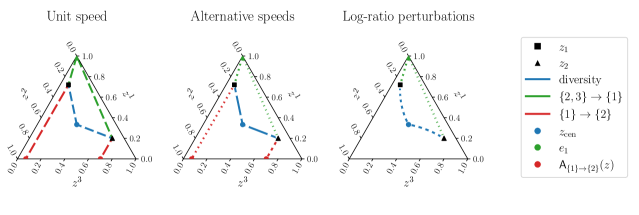
Figure 2: Plots of (left) unit speed perturbations, (middle) alternative speed parametrizations (the diversity perturbation in blue has Gini-speed (see (10)) and multiplicative speed (see (8)) for the amalgamating perturbations in red and green) and (right) log-ratio perturbations for two different initial points $z_{1}$ and $z_{2}$. The types of perturbation are distinguished by color. The dashes represent the speed of the perturbation and are equally spaced in the $\gamma$-domain, so that longer lines correspond to faster speeds. The log-ratio diversity perturbation is not a straight line and does not have the same direction as the centering perturbations.

Example 6 (Diversity in the Aitchison geometry).

Suppose we are interested in the effect of diversifying $z\in(\Delta^{d-1})^{\circ}$. As in Example 5, we can think of such effects as moving towards the center $z_{\mathrm{cen}}$, but now using the Aitchison geometry this corresponds to moving $\mathrm{CLR}(z)$ towards $\mathrm{CLR}(z_{\mathrm{cen}})=0$ along a straight line in CLR-space. This line transformed back to the simplex can be written as

$$\{\mathrm{CLR}^{-1}((1-\gamma)\mathrm{CLR}(z))\mid\gamma\in[0,1]\}.$$

Therefore, computing the diversifying direction in the Aitchison geometry amounts to differentiating the expression above at $\gamma=0$ and normalizing. Applying the chain rule, this yields

$$\partial_{\gamma}\mathrm{CLR}^{-1}((1-\gamma)\mathrm{CLR}(z))^{j}\bigm{|}_{\gamma=0}=\sum_{k\in[d]:k\neq j}z^{j}z^{k}\log\left(\frac{z^{k}}{z^{j}}\right),$$

which can be normalized to a unit $1$-norm vector. The direction of this derivative can be vastly different from the centering direction used in Example 5. To obtain a derivative-isolating reparametrization, we can instead define a unit-speed perturbation on the log-ratio scale, $\widetilde{\psi}:(x,\gamma)\mapsto x-\gamma\frac{x}{\|x\|_{2}}$, and find a reparametrization on this scale. It can be shown that on the log-ratio scale, a derivative-isolating reparametrization is given by $\phi^{L}:x\mapsto-\|x\|_{2}$ and $\phi^{W}(z):=x/\|x\|_{2}$ and we can transform these to reparametrizations of $Z$ by composing with the $\mathrm{CLR}$-transform.

Example 7 (Feature influence in the Aitchison geometry).

Suppose, as in Example 3, we are interested in the effect of increasing the value of a particular component $z^{j}$ of $z\in(\Delta^{d-1})^{\circ}$. For $\mathrm{CLR}(z)\in\mathbb{R}^{d}$ we have a natural notion of increasing $z^{j}$ inherited from $\mathbb{R}^{d}$, namely adding $\gamma$ to $\mathrm{CLR}(z)^{j}$. The derivative of the resulting perturbation on the simplex is for all $k\in[d]$ given by

$$\partial_{\gamma}\mathrm{CLR}^{-1}(\mathrm{CLR}(z)+\gamma e_{j})^{k}\bigm{|}_{\gamma=0}=\mathbbm{1}_{\{k=j\}}z^{j}-z^{j}z^{k}.$$

It is straight-forward to check that the speed and direction of this perturbation match exactly the multiplicative perturbation derived in Example 3. One can therefore view an additive log-ratio perturbation as a multiplicative speed perturbation.

2.2 Perturbation effects on the simplex

To make the discussion more concrete, we now provide several explicit perturbation effects on the simplex using the perturbations constructed in Section 2.1. We motivate each perturbation effect with an example application to showcase potential use cases. A list summarizing all proposed perturbation effects together with their respective derivative-isolating reparametrizations that are used for efficient estimation is provided in Table 2. We encourage practitioners to develop further application-specific perturbations that optimally target the research question they are interested in.

2.2.1 Effects of changes in individual components

As a first example we consider perturbation effects that capture how a response is associated with changes in individual components. These types of effects are, for example, useful as a variable selection tool in compositional data. In Section 4.3, we illustrate this for a human gut microbiome study. For each study participant the body mass index (BMI) $Y$ and their gut microbiome composition $Z$ are measured. We then wants to determine for which microbes a high abundance is associated with a high BMI. The simplex constraint implies that for all coordinates $j$ the conditional independence

$$Y\mbox{${}\perp\mkern-11.0mu\perp{}$}Z^{j}\,|\,Z^{-j}$$ (11)

is trivially satisfied and feature importance or influence measures based on (11) are meaningless. Intuitively, this stems from the fact that changing a single component always requires a change in at least some of the remaining components. We therefore propose – for a fixed component $j$ – to consider perturbations that increase the $j$th component while decreasing all remaining components proportionally. We define the compositional feature influence for the $j$th feature or simply $\mathrm{CFI}^{j}$ as $\tau_{\psi}$ for any directional perturbation with endpoint $e_{j}$. To that end, we already considered these perturbations in Example 3 where we proposed two possible speeds leading to slightly different interpretations of the average perturbation effects: $\mathrm{CFI}^{j}_{\mathrm{unit}}$ is the perturbation that moves at a constant (unit) speed towards the vertex and $\mathrm{CFI}^{j}_{\mathrm{mult}}$ is the perturbation that moves at what we call multiplicative speed (see Example 3 for more intuition on these speeds). $\mathrm{CFI}_{\mathrm{mult}}^{j}$ has previously been proposed by Huang et al. (2023), however without an efficient estimation procedure. Huang et al. (2023) also prove that when a log-contrast regression model is well-specified the $j$th coefficient in the model is equal to $\mathrm{CFI}_{\mathrm{mult}}^{j}$. A crucial difference between unit speed and multiplicative speed perturbations is how they account for observations with $Z^{j}=0$. As the multiplicative speed is $0$ in this case such points do not contribute to $\mathrm{CFI}^{j}_{\mathrm{mult}}$, however, they do contribute to $\mathrm{CFI}^{j}_{\mathrm{unit}}$.

In datasets with many zeros, which is common for example in microbiome data, it can also be interesting to focus only on the effect of zeros in individual components. This can be achieved by considering a binary perturbation $\psi$ given by $\psi(z,1)^{j}=0$ and $\psi(z,1)^{-j}=\mathsf{C}(z^{-j})$. We call the resulting average binary perturbation effect $\lambda_{\psi}$ the compositional knock-out effect for the $j$th feature, or $\mathrm{CKE}^{j}$ for short. The $\mathrm{CKE}^{j}$ allows for a straightforward analysis of zeros in compositional data, which has been a long-standing problem with many existing approaches.

2.2.2 Effects of changes in diversity

As a second example we consider perturbation effects that capture how a response is associated with increases in diversity. Such effects are often relevant in social sciences and econometrics, e.g., when considering racial or income distributions. As we outlined in the introduction, it can be misleading to only model summary statistics of diversity and ignore the remaining compositional structure as this structure can confound the relationship between the diversity measure and the response. Instead, we propose to consider the effect of directional perturbations that push towards $z_{\mathrm{cen}}$ (the centering perturbations defined in Section 2.1.1) and call $\tau_{\psi}$ for such perturbations a compositional diversity influence ($\mathrm{CDI}$). We denote the effect by $\mathrm{CDI}_{\mathrm{unit}}$ if the perturbation has unit speed and by $\mathrm{CDI}_{\mathrm{Gini}}$ if the perturbation was constructed as in Example 5 such that $L$ is equal to the negative Gini coefficient. The construction in Example 5 can be adapted to many popular diversity measures and hence allows practitioners to use their favorite diversity summary statistics. In Section 4.2, we use data from the $1994$ US census to analyze the effect of racial diversity on income and show how $\mathrm{CDI}_{\mathrm{Gini}}$ avoids the confounding caused by naively including the Gini coefficient in a regression.

We do not define a binary centering perturbation here as it requires a positive probability of observing $Z=z_{\mathrm{cen}}$, which is rarely the case.

2.2.3 Effects of amalgamations

As a third example we consider perturbation effects that capture the influence of general amalgamations. As an example, consider a study where data is collected on how individuals spend their time each day (e.g., hours spent sleeping, eating, working, doing sports, etc.) as well as a response variable (e.g., general happiness). Assume now that we want to use this data to investigate the relationship between time spent on sports and happiness. As above, we are again interested in effect of an individual component, so we might consider estimating a $\mathrm{CFI}^{j}$. However, this would capture the effect of increasing time spent on sports while all other activities are down-scaled proportionally. For example, time spent sleeping and eating would both be decreased if time doing sports is increased which is not realistic. To address this, we can instead consider a general $(A\to B)$-amalgamating perturbation (as defined in Section 2.1.1), where $B=\{\text{sport}\}$ and $A$ corresponds to activities which are reduced to make increased time for sports. Perturbing in this fashion keeps the components in $[d]\setminus(A\cup B)$ fixed (e.g., eating and drinking) while down-scaling the activities in $A$. We call directional perturbation effects of this form compositional amalgamation influences, or $\mathrm{CAI}^{A\to B}$ for short. As with the $\mathrm{CFI}^{j}$, we use subscripts to denote the speed of the perturbation, so we have $\mathrm{CAI}_{\mathrm{unit}}^{A\to B}$ and $\mathrm{CAI}^{A\to B}_{\mathrm{mult}}$ (see Example 4).

Analogously, we could be interested in the effect of removing particular activities (e.g. gambling) entirely and spending the time on desirable activities (e.g. sports) while fixing time spent on a third group of activities (e.g. eating, sleeping). We can capture this effect using a binary amalgamating perturbation $\psi$. We call the resulting average binary perturbation effect for $\psi$ an $(A\to B)$-compositional amalgamation effect, or $\mathrm{CAE}^{A\to B}$ for short.

Effect of changes in	Target	Speed $s(z)$	Endpoint $E(z)$	$\phi^{L}(z)$
individual components	$\mathrm{CFI}^{j}_{\mathrm{unit}}$	$1$	$e_{j}$	$-2(1-z^{j})$
	$\mathrm{CFI}^{j}_{\mathrm{mult}}$	$2z^{j}(1-z^{j})$	$e_{j}$	$\log(\frac{z^{j}}{1-z^{j}})$
	$\mathrm{CKE}^{j}$	binary	$e_{j}$	$\mathds{1}_{\{z^{j}=0\}}$
diversity	$\mathrm{CDI}_{\mathrm{unit}}$	$1$	$z_{\mathrm{cen}}$	$-\|z_{\mathrm{cen}}-z\|_{1}$
	$\mathrm{CDI}_{\mathrm{Gini}}$	see (10)	$z_{\mathrm{cen}}$	$-G(z)$, see (9)
amalgamations	$\mathrm{CAI}^{A\to B}_{\mathrm{unit}}$	$1$	$\mathsf{A}_{A\to B}(z)$	$-2\|z^{A}\|_{1}$
	$\mathrm{CAI}^{A\to B}_{\mathrm{mult}}$	$\frac{2\|z^{A}\|_{1}\|z^{B}\|_{1}}{(\|z^{A}\|_{1}+\|z^{B}\|_{1})^{2}}$	$\mathsf{A}_{A\to B}(z)$	$\log\big{(}\tfrac{\|z^{B}\|_{1}}{\|z^{A}\|_{1}}\big{)}$
	$\mathrm{CAE}^{A\to B}$	binary	$\mathsf{A}_{A\to B}(z)$	$\mathds{1}_{\{z^{A}=0\}}$

Table 2: List of perturbation effects considered in this work and what effects they capture. For each perturbation effect the corresponding speed, endpoint and $L$-term of the reparametrization used for efficient estimation is included. All reparametrizations use the canonical direction $v_{E}$ based on the endpoint, see (6). The $W$-term $\phi^{W}(z)$ of the reparametrization is $E(z)$ for the binary effects and $(v_{E}(z),E(z))$ for the directional effects.

2.3 Perturbations as causal quantities

Perturbations are a priori non-causal quantities and should not be confused with (causal) interventions. To make this distinction clear, we now discuss how our perturbation framework can be used for causal inference. Causal models (Pearl, 2009; Rubin, 2005) provide a mathematical framework for modeling changes to the data generating mechanism – often called interventions. In contrast to an (observational) statistical model, which assumes a single observational distribution that generated the data, a causal model additionally postulates the existence of a collection of interventional distributions that describe the data generating mechanism under hypothetical interventions. The power of causal models is that they allow specification of rigorous mathematical conditions under which (parts of) the interventional distributions can be identified (or computed) from the observational distribution. Unlike interventions, perturbations describe hypothetical changes to the predictor space (in this work $\Delta^{d-1}$, but the same ideas hold more generally) and not to the data-generating mechanism. To make this more precise and show how to use perturbations for causal inference, we use the structural causal model (SCM) framework (Pearl, 2009; Bongers et al., 2021). Similar considerations, however, also apply with the potential outcome framework.

As an example, consider the SCM over the variables $(H,Z,Y)\in\mathbb{R}^{q}\times\Delta^{d-1}\times\mathbb{R}$ given by

$$\mathcal{M}:\,\begin{cases}&H\leftarrow\varepsilon_{H}\\ &Z\leftarrow h(H,\varepsilon_{Z})\\ &Y\leftarrow g(H,Z)+\varepsilon_{Y},\end{cases}$$

where $h:\mathbb{R}^{q}\times\mathbb{R}\rightarrow\Delta^{d-1}$ and $g:\mathbb{R}^{q}\times\Delta^{d-1}\rightarrow\mathbb{R}$ are measurable functions and $(\varepsilon_{H},\varepsilon_{Y},\varepsilon_{Z})$ are jointly independent noise terms with expectation zero. The SCM $\mathcal{M}$ generates a distribution over $(H,Y,Z)$ which is called the observational distribution. Intervening corresponds to changing individual structural assignments while keeping everything else fixed such that the modified SCM again induces a distribution – called the interventional distribution. The example SCM $\mathcal{M}$ is a commonly assumed causal structure in which the predictor $Z$ causally precedes the response but is confounded by $H$.

Assume now we observe data generated by $\mathcal{M}$ and are interested in understanding how $Z$ causally affects $Y$. One target parameter might be to consider the expected value of $Y$ under an intervention that sets $Z$ to a fixed value, using do-notation (Pearl, 2009), this can be expressed as $\mathbb{E}[Y\mid\operatorname{do}(Z=z)]=\mathbb{E}[g(z,H)]$. For larger $d$ the full causal relation might be too ambitious of a goal, and it may be more tractable to look at the effect of individual components. Since the vector $Z$ is compositional, one needs to be careful when expressing summary interventions. Perturbations provide a solution to this as they allow us to express sensible ways of changing the predictors. More specifically, let $\psi$ be a perturbation as defined in Definition 1. Then, for all $\gamma\in[0,1]$, consider the intervention $\operatorname{do}(Z=\psi(Z,\gamma))$, which in $\mathcal{M}$ replaces the $Z$-structural assignment by $Z\leftarrow\psi(g(H,\varepsilon_{Z}),\gamma)$. In a similar way as to how we previously used the conditional expectation of $Y$ under the perturbation, we can now use the expected value of $Y$ under the perturbation-induced intervention, i.e., $\mathbb{E}[Y\mid\operatorname{do}(Z=\psi(Z,\gamma))]$. Here, we only consider interventions on the entire compositional vector $Z$, which means that it is not possible to model how causal effects propagate within the composition itself. The corresponding causal versions of the target parameters in Definition 2 are then the causal average binary perturbation effect

$$\lambda_{\psi}^{\operatorname{causal}}:=\frac{\mathbb{E}\big{[}\mathbb{E}\left[Y\,|\,\operatorname{do}(Z=\psi(Z,1))\right]-\mathbb{E}\left[Y\right]\big{]}}{\mathbb{P}(Z\neq\psi(Z,1))}$$

and the causal average directional perturbation effect

$$\tau_{\psi}^{\operatorname{causal}}:=\mathbb{E}\left[\partial_{\gamma}\mathbb{E}\left[Y\,|\,\operatorname{do}(Z=\psi(Z,\gamma))\right]\big{|}_{\gamma=0}\right].$$

Unlike their non-causal versions, the causal average perturbation effects may not be identifiable from the observational distribution. Therefore, to estimate them, we need to make additional causal assumptions. For example, we may assume the variable $(H,Y,Z)$ were generated by an SCM with the same causal structure as $\mathcal{M}$. In that case, if $H$ is observed, the expectation of $Y$ under perturbation induced interventions on $Z$ can be expressed as

$$\mathbb{E}[Y\mid\operatorname{do}(Z=\psi(Z,\gamma))]=\mathbb{E}\big{[}\mathbb{E}[Y\mid Z=\psi(Z,\gamma),H]\big{]},$$ (12)

and hence is identifiable. The formula in (12) is a special case of the adjustment formula (e.g., Pearl, 2009), but other ways of identifying this effect also exist (e.g., propensity score matching). It is easy to adapt the estimators proposed in this work to such settings by conditioning on additional confounding covariates $H$. In particular, starting from the reparametrization into $(L,W)$ one only needs to add additional observed confounders alongside $W$. This is for example done in the numerical experiment in Section 4.2.

Finally, let us shortly discuss under which assumptions the causal and non-causal average perturbation effects coincide. Obviously, one sufficient condition is to assume that

$$\mathbb{E}[Y\mid\operatorname{do}(Z=\psi(Z,\gamma))]=\mathbb{E}[Y\mid Z=\psi(Z,\gamma)].$$ (13)

Such a condition holds by definition whenever $Z$ is an exogenous variable (i.e., does not depend on other variables in its structural assignment) but can also hold more generally. A common assumption to ensure (13) is to assume that $Z$ and $Y$ are not confounded, that is, $Z$ and $Y$ have no common causes (this is known as ignorability in the potential outcome framework). In the SCM $\mathcal{M}$ this would for example mean that $H$ does not exist or either $g$ or $h$ do not depend on $H$. In many cases, this is not satisfied and one should instead carefully argue for which causal assumptions are reasonable and adjust the estimation accordingly, e.g., by conditioning on additional covariates as in (12).

3 Estimating perturbation effects

In this section, we describe how to estimate and test hypotheses about the target parameters $\tau_{\psi}$ and $\lambda_{\psi}$. We will not explicitly restrict ourselves to any one perturbation $\psi$ as the approaches described are agnostic to this choice. However, we will assume that any directional perturbation comes with a derivative-isolating reparametrization $\phi=(\phi^{L},\phi^{W})$ and for any binary perturbation we define $\phi^{L}:z\mapsto\mathbbm{1}_{\{}z=\psi(z,1)\}$ and $\phi^{W}:z\mapsto\psi(z,1)$. This allows us to transform our estimation problem from a compositional data problem where we observe $n$ i.i.d. copies of $(Y,Z)\in\mathbb{R}\times\Delta^{d-1}$ to a generic problem with $n$ observations of $(Y,L,W)$ with $W\in\mathcal{W}$ and $L\in\mathbb{R}$, where our interest lies in the relationship between $Y$ and $L$ when controlling for $W$. We only present an overview of the different estimators in this section and postpone a detailed description of the algorithms and theory to Section 5.

3.1 Efficient estimation using semiparametric theory

We now give a brief introduction to semiparametric estimation of statistical functionals and, in particular, we describe how naive plug-in estimation of target parameters based on nonparametric methods rarely leads to efficient tests and how to remedy this. This perspective is not new and goes back to at least Pfanzagl (1982) with several more recent monographs and reviews (Bickel et al., 1993; Tsiatis, 2006; Chernozhukov et al., 2018; Kennedy, 2023). For illustration, we focus on the estimation of $\tau_{\psi}$, that is, the estimation of

$$\tau_{\psi}=\mathbb{E}[\partial_{\ell}f(\ell,W)\bigm{|}_{\ell=L}],$$

where $f:(\ell,w)\mapsto\mathbb{E}[Y\,|\,L=\ell,W=w]$. A naive approach, which is known as plug-in estimation, is to estimate $\tau_{\psi}$ by first learning a differentiable estimate $\widehat{f}$ of $f$ using all $n$ observations and then computing

$$\widetilde{\tau}_{\psi}:=\frac{1}{n}\sum_{i=1}^{n}\partial_{\ell}\widehat{f}(L_{i},W_{i}).$$

While such an estimate can be consistent, it is rarely asymptotically Gaussian, which invalidates standard asymptotic inference. Using the corresponding plug-in estimate of the asymptotic variance, given by

$$\widetilde{\sigma}^{2}:=\frac{1}{n}\sum_{i=1}^{n}(\partial_{\ell}\widehat{f}(L_{i},W_{i}))^{2}-\widetilde{\tau}_{\psi}^{2},$$ (14)

hence does not provide valid inference (see Figure 3 (left)) as the confidence intervals can be biased or too narrow.

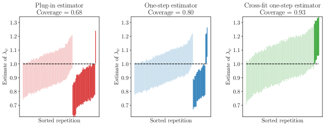
Figure 3: Plot of $95\%$ confidence intervals for a plug-in, one-step and cross-fit one-step estimator of $\lambda_{\psi}$ across 100 repetitions in the partially linear, binary simulation setting described in Section 4.1 with $d=15$ and $n=1000$. The black dashed line indicates the true value of the parameter and we highlight the confidence intervals that do not contain the true parameter. The confidence intervals are ordered first by whether the true value is in the interval, then by the value of the estimate.

There are two main issues with this estimate; (a) repeated usage of the same data for both the estimation of $f$ and the computation of the target (double-dipping) and (b) estimation bias inherited from the bias in $\widehat{f}$. Issue (a) can be resolved by splitting the dataset into two parts of roughly equal size and using the first half to compute $\widehat{f}$ and the second part to compute $\widetilde{\tau}_{\psi}$. To increase finite-sample performance of this splitting procedure, one can swap the roles of the two halves and average the resulting estimates. This procedure is known as cross-fitting. Sometimes it is preferable to split in more than two folds to increase the sample size in the estimation of $\widehat{f}$ and to derandomize the resulting estimate. Issue (b) is more complicated to resolve and requires the machinery of semiparametric theory. One well-established approach is to start from the plug-in estimator and derive a bias-correction, known as a one-step correction, that can be added to the plug-in estimator and weakens the conditions under which the estimator is asymptotically Gaussian. The one-step correction can be found by computing the influence function of the target parameter, which can be thought of as analogous to a derivative when the target parameter is viewed as a function defined on a space of distributions. For more details on this general procedure, see e.g. Kennedy (2023). It can be shown that these bias-corrected estimators are asymptotically efficient, meaning that, at least asymptotically, they have the smallest possible variance of any estimator. Influence functions have already been computed for the target parameters $\tau_{\psi}$ and $\lambda_{\psi}$ that we estimate here and we will describe the details of these estimates in the following sections. Figure 3 contains an illustration of the coverage of confidence intervals resulting from target parameter and variance estimates from the different methods mentioned above.

3.2 Efficient estimation of perturbation effects

In this section, we present our proposals for estimating perturbation effects. We postpone the theoretical analysis and a detailed description of cross-fitting to Section 5 and only provide a high-level overview here. All the presented estimators involve regressions that can be performed by arbitrary (sufficiently powerful) regression methods.

3.2.1 Nonparametric estimation of the binary perturbation effect

Consider a binary perturbation $\psi$ with corresponding perturbation effect $\lambda_{\psi}$ and recall from the arguments of Section 2 that with $L:=\mathbbm{1}_{\{Z=\psi(Z,1)\}}$ and $W:=\psi(Z,1)$, we have that

$$\lambda_{\psi}=\frac{\mathbb{E}\big{[}\mathbb{E}\left[Y\,|\,L=1,W\right]]-\mathbb{E}\left[Y\right]}{\mathbb{P}(L=0)}.$$

The denominator and $\mathbb{E}[Y]$ are both easy to estimate efficiently using their empirical counterparts (the one-step correction term is $0$ for these quantities). The term $\mathbb{E}\big{[}\mathbb{E}\left[Y\,|\,L=1,W\right]]$ in the numerator is trickier and is related to the notion of average predictive effects (e.g., Robins et al., 1994; Chernozhukov et al., 2018; Kennedy, 2023) that has been analyzed extensively in the causal inference literature. The one-step corrected estimator for $\mathbb{E}\big{[}\mathbb{E}\left[Y\,|\,L=1,W\right]]$ is related to the augmented inverse propensity weighted (AIPW) estimator and is given by

$$\frac{1}{n}\sum_{i=1}^{n}\widehat{f}(1,W_{i})+\frac{Y_{i}-\widehat{f}(L_{i},W_{i})}{\widehat{\pi}(W_{i})}L_{i},$$

where $\widehat{f}$ is an estimator of $f:(\ell,w)\mapsto\mathbb{E}[Y\,|\,L=\ell,W=w]$ and $\widehat{\pi}$ is an estimator of the propensity score $\pi:w\mapsto\mathbb{P}(L=1\,|\,W=w)$. An efficient estimator for $\widehat{\lambda}_{\psi}$ is thus

$$\widehat{\lambda}_{\psi}:=\frac{\frac{1}{n}\sum_{i=1}^{n}\widehat{f}(1,W_{i})-Y_{i}+\frac{Y_{i}-\widehat{f}(L_{i},W_{i})}{\widehat{\pi}(W_{i})}L_{i}}{\frac{1}{n}\sum_{i=1}^{n}(1-L_{i})}.$$ (15)

A full algorithm is given in Algorithm 2. It is worth noting that this estimator is sensitive to the estimation of the propensity score $\pi$ which can be difficult when the dimension of $W$ is large or the relationship between $L$ and $W$ is complicated (see Section S3.1 of the supplementary material for an illustration of this).

3.2.2 Nonparametric estimation of the directional perturbation effect

Consider a directional perturbation $\psi$ with a derivative-isolating reparametrization $\phi=(\phi^{L},\phi^{W})$ and the corresponding perturbation effect $\tau_{\psi}$. By the arguments in Section 2, setting $L:=\phi^{L}(Z)$ and $W:=\phi^{W}(Z)$, we have that

$$\tau_{\psi}=\mathbb{E}[\partial_{\ell}\mathbb{E}[Y\,|\,L=\ell,W]\big{|}_{L=\ell}].$$

This quantity is another well-known target of inference; the average partial effect (Newey and Stoker, 1993; Chernozhukov et al., 2022; Klyne and Shah, 2023). The one-step corrected estimator in this setting is given by

$$\widehat{\tau}_{\psi}:=\frac{1}{n}\sum_{i=1}^{n}\partial_{\ell}\widehat{f}(L_{i},W_{i})-\widehat{\rho}(L_{i},W_{i})(Y_{i}-\widehat{f}(L_{i},W_{i}))$$ (16)

where $\widehat{f}$ is a differentiable estimator of $f:(\ell,w)\mapsto\mathbb{E}[Y\,|\,L=\ell,W=w]$ and $\widehat{\rho}$ is an estimate of the conditional score function $\rho$ of $L$ given $W$, that is, an estimate of the function $\rho:(\ell,w)\mapsto\partial_{\ell}\log(p(\ell|w))$ where $p$ denotes the conditional density of $L$ given $W$. A full algorithm for the estimation is given in Algorithm 1 below. Both the estimation of $f$ with computable derivative $\partial_{\ell}f$ and $\rho$ can be challenging and we show in Section 4 that the overall estimator (16) is sensitive to both estimates (see Section S3.1 of the supplementary material for an illustration of this).

For the estimation of $f$ we require that the estimator $\widehat{f}$ is differentiable and with computable derivatives (which additionally need to approximate the true derivative at a sufficiently fast rate). This excludes the direct use of many popular machine learning methods such as random forests or boosted trees. One solution is to start from a potentially non-differentiable pilot estimate of $f$ and smooth it to get a differentiable estimate for which derivatives can be computed. Such a procedure based on kernel-smoothing has been proposed by Klyne and Shah (2023). Here, we use an alternative smoothing method which uses random forests and local polynomials. A full description of our smoothing method is provided in Section S3.3 of the supplementary material. Finally, for the estimation of $\rho$, we follow the proposal in Klyne and Shah (2023) and assume a location-scale model. This requires the estimation of the conditional mean and variance of $L$ given $W$ (referred to as $\eta$ in Algorithm 1). Further details on the location-scale based estimate of $\rho$ is given in Section S3.4 of the supplement.

3.2.3 Partially linear estimation of perturbation effects

While the estimators in the previous sections make only mild assumption on the data generating model, they rely on accurate estimates of quantities that may be difficult to estimate, such as derivatives of densities and regression functions. One way to avoid these complicated estimations is by additionally assuming a partially linear model. For both binary and directional perturbations (with a derivative-isolating reparametrization), we can assume a partially linear model on $L$ and $W$, that is, the existence of $h$ and $\theta$ such that

$$\mathbb{E}[Y\,|\,L,W]=\theta L+h(W).$$ (17)

With this assumption, $\theta$ is exactly equal to the perturbation effect. Efficient estimation of $\theta$ in a partially linear model is a well-studied problem (e.g., Robinson, 1988; Chernozhukov et al., 2018) and one estimator (sometimes referred to as the partialling out estimator) is given by

$$\widehat{\theta}:=\frac{\sum_{i=1}^{n}\{Y_{i}-\widehat{g}(W_{i})\}\{L_{i}-\widehat{m}(W_{i})\}}{\sum_{i=1}^{n}\{L_{i}-\widehat{m}(W_{i})\}^{2}},$$ (18)

where $\widehat{g}$ is an estimator of $g:w\mapsto\mathbb{E}[Y\,|\,W=w]$ and $\widehat{m}$ is an estimator of $m:w\mapsto\mathbb{E}[L\,|\,W=w]$. A full algorithm is given in Algorithm 3. In contrast to the estimators from the previous sections, this estimator only relies on estimating two conditional mean functions. This comes at the expense of assuming that there is no interaction effect between $L$ and $W$ on $Y$ and that the effect of $L$ is linear on $Y$. Even when these assumptions are not satisfied, the estimator may still provide a reasonable estimate of the effect of $L$ on $W$ and we found in our experiments that the estimator is more robust to errors in the estimation of the nuisance functions than the estimators above. In fact, one can show that the quantity $\mathbb{E}[(\mathbb{E}[Y\,|\,L,W]-\theta L-h(W))^{2}]$ is minimized by the population version of the partially linear model estimate, so one can think of the partially linear model as a ‘best approximation’ to a generic nonparametric model (see Proposition S1 in Section S3.1.3 of the supplementary material for a proof of this fact).

4 Numerical experiments

We now present three numerical experiments illustrating the usage and performance of our methods. In Section 4.1 we investigate the performance of the semiparametric estimators discussed in Section 3. In Section 4.2 we analyze the effect of diversity on income based on grouped data from the 1994 US census. In Section 4.3 we investigate variable influence (importance) measures for the prediction of BMI from gut microbiome data. The code for all of our experiments is available at https://github.com/ARLundborg/PerturbationCoDa. For all regressions we use the scikit-learn package (Pedregosa et al., 2011) except for the $\ell^{1}$-penalized log-contrast regression in Section 4.3 where we used the c-lasso package (Simpson et al., 2021).

4.1 Semiparametric estimators

In this section we investigate the performance of the semiparametric estimators outlined in Section 3 with $W$ as a simplex-valued random variable. More specifically, we compare the different approaches of estimating

$$\lambda_{\psi}=\frac{\mathbb{E}\big{[}\mathbb{E}\left[Y\,|\,L=1,W\right]]-\mathbb{E}\left[Y\right]}{\mathbb{P}(L=0)}\quad\text{and}\quad\tau_{\psi}=\mathbb{E}[\partial_{\ell}\mathbb{E}[Y\,|\,L=\ell,W]\big{|}_{L=\ell}]$$

from i.i.d. data $(Y_{1},L_{1},W_{1}),\ldots,(Y_{n},L_{n},W_{n})$. For both types of average perturbation effects we consider the following seven types of estimators.

• NPM: The one-step corrected nonparametric estimators including cross-fitting, i.e., (15) and (16). See Algorithms 1 and 2, with $K=2$, for the detailed binary and directional effect estimators, respectively.

• NPM_no_x: The same estimators as NPM but without cross-fitting.

• NPM_oracle: The same estimators as NPM including cross-fitting but using the true nuisance functions for the one-step-correction (propensity score $\pi$ in the binary case and conditional score function $\rho$ in the directional case). This is an oracle as the true nuisance functions are unknown in practice.

• PLM: The partially least model based estimators in (18) including cross-fitting. See Algorithm 3 with $K=2$ for the detailed estimators.

• PLM_no_x: The same estimators as PLM but without cross-fitting.

• plugin: The naive plugin versions of the NPM estimates. In the binary effect case, the estimator in (15) without the term involving $\widehat{\pi}$ and in the directional effect case, the estimator in (16) without the term involving $\widehat{\rho}$.

• plugin_no_x: The same estimators as plugin but without cross-fitting.

The variance of the NPM and PLM estimates is computed based on the provided algorithms for the NPM and PLM methods while the variance for the plugin is estimated using an estimator akin to the one given in (14). Each estimator above is itself based on multiple of the regression estimates $\widehat{f}$, $\widehat{\pi}$, $\widehat{g}$ and $\widehat{m}$ and NPM and NPM_no_x additionally on the score estimate $\widehat{\rho}$. For the regression estimates, we use a $5$-fold cross-validation based estimator which for each fit selects among the following three models: a simple model that predicts the mean of the outcome (or the proportion of each class for binary classification), a random forest with $250$ trees with trees grown to a maximum depth of $2$ and a random forest with $250$ trees and no depth restriction. For the score estimator we use the location-scale based estimator described in Section S3.4 of the supplement, that uses the same $5$-fold cross-validated regression estimator for the location and scale nuisance regressions.

We consider four data generating models each with varying sample size $n\in\{250,1000,4000\}$ and predictor dimension $d\in\{3,15,75\}$. In all settings, we let $W$ be uniformly distributed on $\Delta^{d-2}$, denote by $\mathrm{med}_{W_{1}}$ the population median of $W_{1}$ and $\sigma_{W_{1}}^{2}$ the variance of $W_{1}$ and define $B(W_{1}):=\mathbbm{1}_{\{W_{1}>\mathrm{med}_{W_{1}}\}}$. We then consider the following four generative models

• Binary $L$ with partially linear $Y$:

  $$L=U_{0}(1-B(W_{1}))+U_{1}B(W_{1})\quad\text{and}\quad Y=L+\sigma_{W_{1}}^{-1}W_{1}+\varepsilon$$

• Binary $L$ with nonparametric $Y$:

  $$L=U_{0}B(W_{1})+U_{1}B(W_{1})\quad\text{and}\quad Y=\frac{7}{5}LB(W_{1})+\sigma_{W_{1}}^{-1}W_{1}+\varepsilon$$

• Continuous $L$ with partially linear $Y$:

  $$L=B(W_{1})+\xi\quad\text{and}\quad Y=L+B(W_{1})+\varepsilon$$

• Continuous $L$ with nonparametric $Y$:

  $$L=B(W_{1})+(1+B(W_{1}))\xi\quad\text{and}\quad Y=2B(W_{1})L+B(W_{1})+\varepsilon$$

The noise variables $U_{0}\sim\mathrm{Bern}(0.8)$, $U_{1}\sim\mathrm{Bern}(0.5)$, $\varepsilon\sim\mathcal{N}(0,1)$ and $\xi\sim\mathcal{N}(0,1)$ are all sampled independently (and independent of $W$). The true value of $\lambda$ in the binary $L$ settings and $\tau$ in the continuous $L$ settings is $1$. For each setting we simulate data and compute an estimate with a corresponding asymptotic $95\%$ confidence interval using each of the methods described above. We repeat the experiment $100$ times and compute coverage rates of the $95\%$ confidence intervals for $d=15$ in Figure 4 while coverage rates for $d=3$ and $d=75$ are reported in Section S4.2 of the supplementary material.

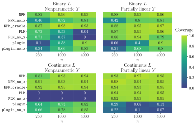
Figure 4: Estimated coverage rates of the $95\%$ confidence intervals for each different estimation procedures over $100$ repetitions for each of the settings described in Section 4.1 with $d=15$. PLM works well if $Y$ follows a partially linear model, but can fail if this assumption is not satisfied as in the nonparametric $Y$ setting. NPM works in both settings but can be less robust for small sample sizes. Further, it can be seen that the plugin estimator and the estimators without cross-fitting do not lead to correct coverage in some of these settings.

In all settings we see that the partially linear model works well when it is well-specified but can fail when the partially linear assumption is violated. We see that the plugin estimator generally performs worse than the one-step estimator but this disparity is reduced for large $n$. In many cases cross-fitting is not a necessity, however, in some settings cross-fitting does positively impact the performance of the tests, e.g. for $n=1000$ and binary $L$. In the cases where cross-fitting is not necessary, it does not seem to negatively impact the performance of the test.

4.2 Compositional confounding in relationship between income and race

In this section we provide an example based on real data that illustrates how failing to adjust for compositional confounding can lead to incorrect conclusions about effects of compositional variables. We consider the ‘Adult’ dataset available from the UCI machine learning repository (Becker and Kohavi, 1996). This dataset is based on an extract from the 1994 US Census database and consists of data on 48,842 individuals. The response variable in the data, compensation, is a binary variable where $0$ and $1$ encode whether an individual makes below or above 50,000 USD per year, respectively. Additionally, we consider the demographic features age (numeric, between 17 and 90), education (categorical, with 16 categories), sex (binary, $0$ encoding male and $1$ female) and race (categorical, with categories ’White’, ’Black’ and ’Other’).

We now use this individual-level data to construct community-level datasets by artificially grouping individuals together. This allows us to construct settings, where there is a known dependence between the racial diversity of the communities and the response variable. As we show below, this illustrates the potential pitfalls of ignoring compositional structure in the data and how the approach based on perturbations solves these issues. More specifically, we group all individual-level observations into groups of around $50$ individuals. We then create a new response variable $Y\in[0,1]$ by averaging the individual-level compensation in each group. Similarly, we create a predictor variable $X\in\mathbb{R}\times[0,1]\times\{1,\dots,16\}$ by averaging age and sex and selecting the majority class of the categorical variable education (breaking ties randomly). Finally, we create a compositional predictor $Z\in\Delta^{2}$ by computing the proportions of ‘White’, ‘Black’ and ‘Other’ individuals in each group. To ensure, a (partially) known effect of increased racial diversity on compensation, we construct three categories of groups (0, 1 and 2). We construct these categories in two different ways:

• Grouping by race and education: Groups in category 1 are sampled to be similarly diverse and with lower educational levels than the total population and category 2 groups are sampled to be more diverse and with higher educational levels than the total population. The groups in category 0 consist of groups constructed randomly from the remaining individuals.

• Grouping by race and compensation: Groups in category 1 are sampled to be similarly diverse and with lower average compensation than the total population and category 2 groups are sampled to be more diverse and with higher average compensation than the total population. The groups in category 0 consist of groups constructed randomly from the remaining individuals.

We then sample groups from each category, using a weighted sampling approach described in detail in Section S4.3 of the supplementary material. This results in $978$ observations with $811$ in category $0$, $92$ in category $1$ and $75$ in category $2$ when grouping on education and $782$ in category $0$, $129$ in category $1$ and $67$ in category $2$ when grouping on compensation. For each type of grouping the racial composition for the resulting groups is illustrated in the top half of Figure 5. In both cases we expect that – by construction – there is a positive effect of increased diversity on compensation (for the grouping by race and education this is because education is positively associated with compensation).

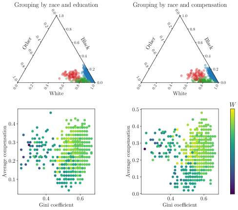
Figure 5: Top: Racial compositions for both types of grouping in a ternary plot. Each point corresponds to one group and is colored according to which category it belongs to ($0$ in blue, $1$ in green and $2$ in red).
Bottom: Plot of average compensation per group ($Y$) against Gini coefficient colored by the value of $W=(z_{\mathrm{cen}}-Z)/\|z_{\mathrm{cen}}-Z\|_{1}$ ($W$ takes values in a $1$-dimensional subset of $\mathbb{R}^{3}$). Depending on the color the dependence between $Y$ and the Gini coefficient changes.

Based on the two constructed community-level datasets, we now compare a naive approach that neglects the simplex structure and is applied in the literature (e.g. Richard (2000); Richard et al. (2007); Lu et al. (2015); Paarlberg et al. (2018)) with the perturbation-based approach. The naive approach summarizes racial diversity in a single measure, here we use minus the Gini coefficient $L=-\frac{1}{2d}\sum_{j=1}^{d}\sum_{k=1}^{d}|Z^{j}-Z^{k}|$ as in Example 5, for which large values correspond to high diversity, and estimate associations between this measure and the average compensation $Y$. We call the method that regresses $Y$ on $L$ linearly naive_diversity. This estimator can easily be adapted to also adjust for the additional covariates $X$, the racial composition $Z$ or both under a partially linear model assumption. The point estimates together with asymptotic confidence intervals (based on an efficient partialling out estimator like the estimator in (3)) are provided in Table 3. The naive estimator that conditions either on the empty set or on $X$ both result in significant negative effects which by construction of the datasets is incorrect. Furthermore, additionally conditioning on $Z$, leads to an ill-conditioned estimator as $Z$ is now a perfect predictor of the diversity measure. This is also visible in the large resulting confidence intervals. While we here constructed the groups in a way to highlight how compositional confounding can be misleading, we believe that this type of confounding is likely also present in real-world settings as groupings are often confounded (e.g., educational levels may well be correlated with race and average compensation in actual communities).

These pitfalls can be avoided with a perturbation-based analysis. In this setting, we propose to apply $\mathrm{CDI}_{\mathrm{Gini}}$ with and without conditioning on the additional covariates $X$. The results are also shown in Table 3. As desired one gets significant positive effects with this method as it is adapted to the simplex. Interestingly, for $\mathrm{CDI}_{\mathrm{Gini}}$ that adjusts for $X$ the effect disappears for the grouping based on education. This is expected because the association between diversity and compensation was constructed based on education which is also part of $X$.

Method	Grouping on education		Grouping on compensation
	Estimate	$95\%$ CI	Estimate	$95\%$ CI
naive_diversity	${\color[rgb]{0.83984375,0.15234375,0.15625}\mathbf{-0.082}}$	$(-0.144,-0.019)$	${\color[rgb]{0.83984375,0.15234375,0.15625}\mathbf{-0.120}}$	$(-0.194,-0.046)$
$\texttt{naive\_diversity}\,|\,Z$	$-0.219$	$(-1.226,0.788)$	$-0.668$	$(-1.916,0.580)$
$\texttt{naive\_diversity}\,|\,X$	${\color[rgb]{0.83984375,0.15234375,0.15625}\mathbf{-0.085}}$	$(-0.142,-0.027)$	${\color[rgb]{0.83984375,0.15234375,0.15625}\mathbf{-0.106}}$	$(-0.179,-0.034)$
$\texttt{naive\_diversity}\,|\,X,Z$	$-0.111$	$(-0.902,0.680)$	$0.409$	$(-0.403,1.220)$
$\mathrm{CDI}_{\mathrm{Gini}}$	${\color[rgb]{0.171875,0.62890625,0.171875}\mathbf{0.233}}$	$(0.060,0.406)$	${\color[rgb]{0.171875,0.62890625,0.171875}\mathbf{0.614}}$	$(0.429,0.799)$
$\mathrm{CDI}_{\mathrm{Gini}}\,|\,X$	$0.071$	$(-0.049,0.191)$	${\color[rgb]{0.171875,0.62890625,0.171875}\mathbf{0.611}}$	$(0.455,0.768)$

Table 3: Table of estimates in the ‘Adult’ data experiment. Bold numbers indicate significance at a $5\%$ level, red indicates a negative effect, while green indicates a positive effect of diversity. The naive_diversity method indicates that either there is a significant negative or a highly uncertain effect of diversity on compensation despite the fact that the data is constructed with a positive effect of diversity. The CDI correctly identifies this effect.

4.3 Variable influence measures when predicting BMI from gut microbiome

In this section, we analyze the ‘American Gut’ (McDonald et al., 2018) dataset which contains a collection of microbiome measurements and metadata from over 10,000 human participants. We use the pre-processed version used in Bien et al. (2021) (available at https://github.com/jacobbien/trac-reproducible/tree/main/AmericanGut). Our focus is on the relationship between body mass index (BMI) and gut microbiome composition at the species-level and our primary goal is to determine which species are important for predicting BMI. We consider the subset of individuals from the United States with BMI between 15 and 40, height between 145 and 220 cm and age above 16 years. To reduce the dimensionality of the microbiome composition (i.e., the number of species), we perform an initial variable screening and only include species that appear in at least $10\%$ of the observations and where the mean abundance is greater than $10^{-4}$ (this is after scaling the absolute counts by the total number of reads for each observation). The resulting dataset consists of 4,581 observations of $\mathrm{BMI}$ measurements $Y\in\mathbb{R}$ and the relative abundances of $561$ microbial species $Z\in\Delta^{560}$.

We begin by evaluating, how sensitive the proposed perturbation effect estimates are with respect to the employed nuisance function estimators. To this end, we consider three different regression methods: random forest (rf), neural network (mlp) and kernelized support vector regression using an RBF kernel (svr). Each of the regressions is combined with a grid-search cross-validation to automatically tune the hyperparameters of each method. For each of the three regression methods and all the species we then compute $\mathrm{CFI}_{\mathrm{mult}}$, $\mathrm{CFI}_{\mathrm{unit}}$ and $\mathrm{CKE}$ using the estimator based on a partially linear model and the $\mathrm{CKE}$ using the nonparametric estimator. As baselines, we additionally compute a nonparametric $R^{2}$ (Williamson et al., 2021) and permutation importance (Breiman, 2001). Figure 6 shows the Spearman correlation between the estimates from the different regression methods.

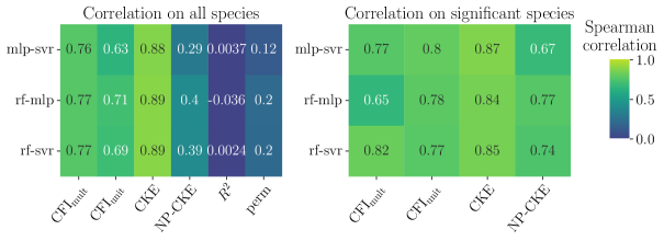
Figure 6: Spearman correlations of variable importance measures computed on each feature using different regressions. On the left, these are computed on all $561$ features and on the right they are computed on the subset of features where at least one of the two methods deems the effect significant at a $5\%$ level. The $R^{2}$ and permutation methods do not come with significance tests and are therefore omitted from the right plot.

While the average perturbation effect estimates which are specifically tailored to the compositional setting are consistent across different regression methods, the permutation and $R^{2}$ measures are – unsurprisingly – not. The population version of the nonparametric $R^{2}$ is always $0$, so the estimates are essentially mean zero random noise that depends on the estimator. For the permutation measure the inconsistency comes the fact that the permuted data inherently leave the support of the simplex, making the resulting influence measure highly dependent on how the regression methods extrapolate. Unfortunately, due to a lack of alternatives, it is still common to use these types feature importance or influence measures in microbiome science (e.g., Marcos-Zambrano et al., 2021). Furthermore, the results show that the nonparametric estimator of the CKE is less well-behaved than the other estimators based on the partially linear model. One reason for this could be that dividing by the propensity score estimator results in a more unstable estimate, particularly when the propensity score is poorly estimated.

Next, we empirically demonstrate that simply ignoring the simplex constraint is not an option. To this end we consider a standard approach for estimating effects of coordinates for unconstrained Euclidean data. More specifically, we compare the proposed $\theta_{j}=\mathrm{CFI}_{\mathrm{unit}}^{j}$ (with estimator based on the partially linear model) with a similar estimator but based on the partially linear model $\mathbb{E}[Y\mid Z]=\theta_{j}Z^{j}+h(Z^{-j})$ in which the parameter $\theta_{j}$ is unidentified due to the simplex constraint. For both methods we use a regression estimator that uses cross-validation to select the best estimator out of a linear regression, random forest and support vector regression. As expected the results from the estimator that ignores the simplex structure are meaningless; for example, $\mathrm{var}(Z^{j})\widehat{\theta}_{j}^{2}/\mathrm{var}(Y)$, a proxy for the variance explained by the linear effect, is larger than $10^{17}$ for all species. In contrast, for $\mathrm{CFI}_{\mathrm{unit}}$ these values lie between $10^{-7}$ and $1.6$.

We now analyze different types of average perturbation effects and compare them with the commonly used log-contrast based analysis. We fit both a standard log-contrast regression and an $\ell^{1}$-penalized log-contrast regression and then use the coefficients as feature influences. Since the log-contrast model is only defined on the open simplex, that is, it does not permit zeros in the data, one usually adds a ‘pseudocount’ to each observation before rescaling to the simplex. We follow a standard recommendation and use the minimum non-zero observation of $Z$ divided by $2$ (this is not required for the perturbation-based measures). To investigate how the log-contrast approach compares to the perturbation-based approach, we plot the most significant hits using $\mathrm{CFI}_{\mathrm{mult}}$ (with random forests as regression method) and a log-contrast regression model in the top row of Figure 7. These are comparable quantities since $\mathrm{CFI}_{\mathrm{mult}}^{j}$ is equal to the $j$th coefficient in a log-contrast model when it is correctly specified and no zeros are present. We omit plotting the $\ell^{1}$-penalized log-contrast estimates as these are broadly similar to the standard log-contrast estimates in this example. We also plot a marginal effect of $L=\log(Z^{j}/(1-Z^{j}))$ which corresponds to predicting $Y$ using OLS on $L$ and correcting for the presence of zeros as we mention in Remark 1. The results with corresponding $95\%$-confidence intervals are given in the top row of Figure 7; top $10$ most significant species sorted according to significance of $\mathrm{CFI}_{\mathrm{mult}}$ (left) and according to log-contrast coefficients (right).

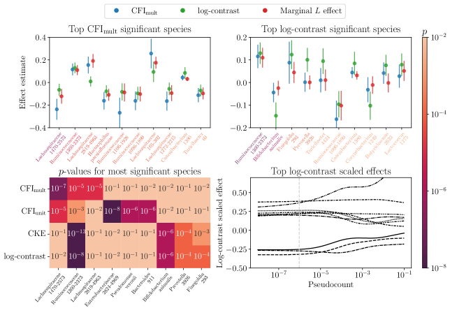
Figure 7: Effect estimates for the $10$ most significant (smallest $p$-value) species from $\mathrm{CFI}_{\mathrm{mult}}$ (top left) and a log-contrast model with pseudocount equal to minimum non-zero observation of $Z$ over $2$ (top right). The labels are colored by the size of the $p$-value. The first $5$ species remain below $0.05$ after Bonferroni-correction for $\mathrm{CFI}_{\mathrm{mult}}$ while this is only true for $2$ for the log-contrast model. The bottom left plot shows the $p$-values from different methods for the three most significant species from each method. We see that the log-contrast model is mostly selecting the same species as the $\mathrm{CKE}$ which explicitly captures effects of zeros. The bottom right plot shows the log-contrast estimates scaled by the standard deviation of $\log(Z^{j}+\text{pseudocount})$ for the species listed on the top right plot as a function of the added pseudocount with the grey dashed line indicating the pseudocount used in the remaining experiments. We see that the relative influences of the different species is highly contingent on the pseudocount.

While the effects overlap for some of the features, there are also significant differences. To further illustrate these differences, we present the $p$-values from $\mathrm{CFI}_{\mathrm{mult}}$, $\mathrm{CFI}_{\mathrm{unit}}$, $\mathrm{CKE}$ and the log-contrast method for several species in the bottom left of Figure 7. From these $p$-values, we can see that the log-contrast and $\mathrm{CKE}$ are highly correlated and appear to be selecting similar species. This is despite the fact that the log-contrast model is supposed to model the continuous effect of each species. The similarities to the $\mathrm{CKE}$ hence indicates (likely due to the pseudocounts) that the log-contrast coefficients are instead capturing the effects of presence and absence of species. To further investigate this, for different values of pseudocounts we plot log-contrast estimates (scaled by the standard deviation of $\log(Z^{j}+\text{pseudocount})$) in the bottom right of Figure 7. This further highlights the dependence of the log-contrast coefficients on the used pseudocount. The fact that the perturbation-based effects explicitly account for zeros and allow us to distinguish between continuous effects (e.g., $\mathrm{CFI}_{\mathrm{unit}}$ or $\mathrm{CFI}_{\mathrm{mult}}$) and presence/absence effects $\mathrm{CKE}$ are an important feature of the perturbation-based approach. In Section S4.4 of the supplementary material we provide an additional plot like the top row of Figure 7 which illustrates the significant hits of $\mathrm{CFI}_{\mathrm{unit}}$ and $\mathrm{CKE}$ when compared to estimates using $\mathrm{CFI}_{\mathrm{mult}}$.

5 Theoretical analysis of estimators

In this section we prove asymptotic normality uniformly over large classes of distributions for each of the three estimation methods described in Section 3; nonparametric estimation of $\tau_{\psi}$, nonparametric estimation of $\lambda_{\psi}$ and by means of estimating $\theta$ in the partially linear model (17). These results are derived using standard proof techniques from the semiparametric literature and likely exist individually in similar form elsewhere (e.g., Klyne and Shah, 2023; Chernozhukov et al., 2018). We do not claim that any of the derived asymptotic results are novel or surprising but include them for completeness and to motivate the precise form of the estimators and their corresponding variance estimates.

We start from a given perturbation $\psi$ and a corresponding reparametrization $\phi:\mathcal{Z}\rightarrow\mathbb{R}\times\mathcal{W}$ which reparametrizes $Z$ into $(L,W):=(\phi^{L}(Z),\phi^{W}(Z))$ and assume that $(L,W)$ satisfy (2) if $\psi$ is a binary perturbation and that $\phi$ is derivative-isolating if $\psi$ is a directional perturbation. Our goal is now to use the estimation procedures discussed in Section 3 to estimate the average perturbation effects (i.e., $\tau_{\psi}$ or $\lambda_{\psi}$) consistently and construct asymptotically valid confidence intervals for the estimates. To construct asymptotically valid confidence intervals, we estimate both the target parameter and its variance and then show that the resulting standardized estimators are asymptotically normal with a uniform convergence rate over the class of possible distributions of the data. Distributionally uniform results are desirable here as they ensure uniform coverage guarantees of the confidence intervals. The following result shows uniform asymptotic normality of each of the three estimation procedures.

Theorem 1 (Uniform asymptotic normality).

Let $\mathcal{P}$ denote a class of distributions of $(Y,L,W)\in\mathbb{R}\times\mathbb{R}\times\mathcal{W}$ and assume we are in one of the following settings.

1. Nonparametric directional effect estimation: Assumption 1 and $(\widehat{\beta},\widehat{\sigma}^{2}_{\beta}):=(\widehat{\tau},\widehat{\sigma}^{2}_{\tau})$ from Algorithm 1.

2. Nonparametric binary effect estimation: Assumption 2 and $(\widehat{\beta},\widehat{\sigma}^{2}_{\beta}):=(\widehat{\lambda},\widehat{\sigma}^{2}_{\lambda})$ from Algorithm 2.

3. Effect estimation using a partially linear model: Assumption 3 and $(\widehat{\beta},\widehat{\sigma}^{2}_{\beta}):=(\widehat{\theta},\widehat{\sigma}^{2}_{\theta})$ from Algorithm 3.

Then, letting $\Phi$ denote the cumulative distribution function of the standard normal distribution, it holds that

$$\lim_{n\to\infty}\sup_{P\in\mathcal{P}}\sup_{x\in\mathbb{R}}\left|\mathbb{P}_{P}\left(\frac{\sqrt{n}}{\widehat{\sigma}_{\beta}}(\widehat{\beta}-\beta_{P})\leq x\right)-\Phi\left(x\right)\right|=0.$$

The result is proven in Section S5 of the supplementary material. In the following three sections, we go over each of the settings (a), (b) and (c) individually and provide the required assumptions and detailed algorithms for the target parameter and variance. For the remainder of this section, we omit $\psi$-subscripts for simplicity and use the following notation to help us express the uniformly asymptotic results rigorously. Let $(X_{P,n})_{n\in\mathbb{N},P\in\mathcal{P}}$ denote a family of sequences of random variables indexed by $\mathcal{P}$. For a nonnegative sequence $(a_{n})_{n\in\mathbb{N}}$ we write $X_{P,n}=o_{\mathcal{P}}(a_{n})$ if for all $\epsilon>0$ it holds that

$$\lim_{n\to\infty}\sup_{P\in\mathcal{P}}\mathbb{P}_{P}(|X_{P,n}|\geq a_{n}\epsilon)=0,$$

that is, $X_{P,n}/a_{n}$ converges to $0$ in probability uniformly over $\mathcal{P}$. We also write $X_{P,n}=O_{\mathcal{P}}(a_{n})$ if for all $\epsilon>0$ there exist $M_{\epsilon}>0$ and $N_{\epsilon}\in\mathbb{N}$ such that

$$\sup_{n\geq N_{\epsilon}}\sup_{P\in\mathcal{P}}\mathbb{P}_{P}(|X_{P,n}|\geq a_{n}M)<\epsilon,$$

that is, $X_{P,n}/a_{n}$ is bounded in probability for large $n$. When we write conditional expectations given a fitted regression function $\widehat{f}$ we mean a conditional expectation given the random variables used to fit $\widehat{f}$ and any additional randomness involved in the fitting.

5.1 Nonparametric estimation for directional effects

We begin with the nonparametric estimation of a directional perturbation effect $\tau$ corresponding to Theorem 1 (a). A high-level overview of this estimation was given in Section 3.2.2. More formally, assume we have a dataset of $n$ i.i.d. copies of $(Y,L,W)$, a differentiable regression method $\widehat{f}$ for the conditional expectation $(\ell,w)\mapsto\mathbb{E}[Y\,|\,L=\ell,W=w]$, a score estimation method $\widehat{\rho}$ for the score $(\ell,w)\mapsto\partial_{\ell}\log(p(\ell\,|\,w))$, where $p$ denotes the conditional density of $L$ given $W$ with corresponding nuisance function estimation method $\widehat{\eta}$ (in our experiments, we assume a location-scale model and thus the nuisance functions are estimators of the conditional mean and variance of $L$ given $W$, see Section S3.4 in the supplementary material). We can then compute the estimator $\widehat{\tau}$ of $\tau$ and its corresponding variance estimate $\widehat{\sigma}_{\tau}^{2}$ as described in Algorithm 1 using a user-specified number of splits $K$ in the cross-validation.

Algorithm 1 Nonparametric estimation of $\tau$

1:Input: Data $(Y_{i},L_{i},W_{i})_{i\in[n]}$, number of folds $K$, differentiable regression method $\widehat{f}$, score estimation method $\widehat{\rho}$ and nuisance function estimate $\widehat{\eta}$.

2:Split indices $\{1,\dots,n\}$ into $K$ disjoint sets $I_{1},\dots,I_{K}$ of (roughly) equal size.

3:For $k\in[K]$, split $I_{k}$ into $I_{k,0}$ and $I_{k,1}$ of (roughly) equal size and set $I_{-k}:=\cup_{k^{\prime}\neq k}I_{k^{\prime}}$.

4:for $k=1,\dots,K$ do

5:     Regress $Y$ on $(L,W)$ using $I_{-k}$ yielding regression estimate $\widehat{f}_{k}$.

6:     Fit nuisance function estimates $\widehat{\eta}_{k}$ using $I_{-k}$.

7:     for $r=0,1$ do

8:         Fit $\widehat{\rho}_{k,r}$ using $I_{k,(1-r)}$ and the nuisance function estimate $\widehat{\eta}_{k}$.

9:         Set $\widehat{\tau}_{k,r}:=|I_{k,r}|^{-1}\sum_{i\in I_{k,r}}\partial_{\ell}\widehat{f}_{k}(L_{i},W_{i})-\widehat{\rho}_{k,r}(L_{i},W_{i})\{Y_{i}-\widehat{f}_{k}(L_{i},W_{i})\}$.

10:         Set $\widehat{\nu}_{k,r}:=|I_{k,r}|^{-1}\sum_{i\in I_{k,r}}\left(\partial_{\ell}\widehat{f}_{k}(L_{i},W_{i})-\widehat{\rho}_{k,r}(L_{i},W_{i})\{Y_{i}-\widehat{f}_{k}(L_{i},W_{i})\}\right)^{2}$.      

11:return $\widehat{\tau}:=\frac{1}{2K}\sum_{k=1}^{K}\sum_{r=0}^{1}\widehat{\tau}_{k,r}$ and $\widehat{\sigma}^{2}_{\tau}:=\frac{1}{2K}\sum_{k=1}^{K}\sum_{r=0}^{1}\widehat{\nu}_{k,r}-\widehat{\tau}^{2}$.

To obtain the result in Theorem 1 (a), we require that the estimation methods $\widehat{f}$ and $\widehat{\rho}$ converge sufficiently fast and that the class of distributions $\mathcal{P}$ satisfies several regularity conditions.

Assumption 1.

Assume that for all $P\in\mathcal{P}$ and $w\in\mathcal{W}$, the conditional distribution of $L$ given $W=w$ has a density with respect to Lebesgue measure and denote it by $p_{P}(\cdot\,|\,w)$. For all $P\in\mathcal{P}$ define $f_{P}:\phi(\mathcal{Z})\to\mathbb{R}$ for all $(\ell,w)\in\phi(\mathcal{Z})$ by $f_{P}(\ell,w):=\mathbb{E}_{P}[Y\,|\,L=\ell,W=w]$ and assume that for almost all $(\ell,w)\in\phi(\mathcal{Z})$ both $p_{P}(\cdot\,|\,w)$ and $f_{P}(\cdot,w)$ are differentiable at $\ell$. Define $\tau_{P}:=\mathbb{E}_{P}[\partial_{\ell}f_{P}(\ell,W)\bigm{|}_{\ell=L}]$ and $\rho_{P}:\phi(\mathcal{Z})\to\mathbb{R}$ for all $(\ell,w)\in\phi(\mathcal{Z})$ by $\rho_{P}(\ell,w):=\partial_{\ell}\log(p_{P}(\ell\,|\,w))$.

Let $(Y_{1},L_{1},W_{1}),\dots,(Y_{3n},L_{3n},W_{3n})$ denote $3n$ i.i.d. copies of $(Y,L,W)$ and define the training datasets $\mathcal{A}:=\{(Y_{n+1},L_{n+1},W_{n+1}),\dots,(Y_{2n},L_{2n},W_{2n})\}$ and $\mathcal{B}:=\{(Y_{2n+1},L_{2n+1},W_{2n+1}),\dots,(Y_{3n},L_{3n},W_{3n})\}$. Let $\widehat{f}$ denote a differentiable estimator of $f_{P}$ based on $\mathcal{A}$, let $\widehat{\eta}$ denote an estimator of a nuisance function relevant for the estimation of $\rho_{P}$ based on $\mathcal{A}$ and let $\widehat{\rho}$ denote an estimator of $\rho_{P}$ based on $\mathcal{B}$ and using the nuisance function estimate $\widehat{\eta}$. Finally, assume there exist constants $\delta,c,C>0$ such that

1. for all $P\in\mathcal{P}:\quad$ $\max\{\mathbb{E}_{P}[|Y|^{4+\delta}],\mathbb{E}_{P}[|\rho_{P}(L,W)|^{4+\delta}],\mathbb{E}_{P}[|\partial_{\ell}f_{P}(L,W)|^{2+\delta}],\mathrm{var}_{P}(Y\,|\,L,W)\}\leq C$

2. for all $P\in\mathcal{P}:\quad$ $\min\{\mathrm{var}_{P}(Y\,|\,L,W),\mathbb{E}_{P}[\rho_{P}(L,W)^{2}]\}\geq c$

3. $\mathbb{E}_{P}\left[\left(\widehat{f}(L_{1},W_{1})-f_{P}(L_{1},W_{1})\right)^{4}\,|\,\,\widehat{f}\,\right]=o_{\mathcal{P}}(1)$

4. $\mathbb{E}_{P}\left[\left(\partial_{\ell}\widehat{f}(L_{1},W_{1})-\partial_{\ell}f_{P}(L_{1},W_{1})\right)^{2}\,|\,\,\widehat{f}\,\right]=o_{\mathcal{P}}(1)$

5. $\frac{1}{n}\sum_{i=1}^{n}\left(\widehat{\rho}(L_{i},W_{i})-\rho_{P}(L_{i},W_{i})\right)^{2}=o_{\mathcal{P}}(1)$

6. $\left(\frac{1}{n}\sum_{i=1}^{n}\left\{\widehat{f}(L_{i},W_{i})-f_{P}(L_{i},W_{i})\right\}^{2}\right)\left(\frac{1}{n}\sum_{i=1}^{n}\left\{\widehat{\rho}(L_{i},W_{i})-\rho_{P}(L_{i},W_{i})\right\}^{2}\right)=o_{\mathcal{P}}(n^{-1})$

5.2 Nonparametric estimation for binary effects

We now present the algorithm and conditions required for the nonparametric estimation of the binary perturbation effect $\lambda$ corresponding to Theorem 1 (b). A high-level overview of this estimation was provided in Section 3.2.1. More formally, assume we have a dataset of $n$ i.i.d. copies of $(Y,L,W)$, a regression method $\widehat{f}$ for the conditional expectation $(\ell,w)\mapsto\mathbb{E}[Y\,|\,L=\ell,W=w]$ and propensity score estimator $\widehat{\pi}$ for the propensity score $w\mapsto\mathbb{P}(L=1\,|\,W=w)$. We can then compute the estimator $\widehat{\lambda}$ of $\lambda$ and its corresponding variance estimate $\widehat{\sigma}^{2}_{\lambda}$ as described in Algorithm 2 using a user-specified number of splits $K$ in the cross-validation.

Algorithm 2 Nonparametric estimation of $\lambda$

1:Input: Data $(Y_{i},L_{i},W_{i})_{i\in[n]}$, number of folds $K$, regression method $\widehat{f}$ and propensity score estimator $\widehat{\pi}$.

2:Split indices $\{1,\dots,n\}$ into $K$ disjoint sets $I_{1},\dots,I_{K}$ of (roughly) equal size.

3:For $k\in[K]$, set $I_{-k}:=\cup_{k^{\prime}\neq k}I_{k^{\prime}}$.

4:for $k=1,\dots,K$ do

5:     Regress $Y$ on $(L,W)$ using $I_{-k}$ yielding regression estimate $\widehat{f}_{k}$.

6:     Regress $L$ on $W$ using $I_{-k}$ yielding propensity score function $\widehat{\pi}_{k}$.

7:     Set $\widehat{\kappa}_{k}:=|I_{k}|^{-1}\sum_{i\in I_{k}}\widehat{f}_{k}(1,W_{i})-Y_{i}+\frac{Y_{i}-\widehat{f}_{k}(L_{i},W_{i})}{\widehat{\pi}_{k}(W_{i})}L_{i}$.

8:     Set $\widehat{\nu}_{k}:=|I_{k}|^{-1}\sum_{i\in I_{k}}\left(\widehat{f}_{k}(1,W_{i})-Y_{i}+\frac{Y_{i}-\widehat{f}_{k}(L_{i},W_{i})}{\widehat{\pi}_{k}(W_{i})}L_{i}\right)^{2}$.

9:Set $\widehat{p}:=\frac{1}{n}\sum_{i=1}^{n}1-L_{i}$.

10:Set $\widehat{\kappa}:=\frac{1}{K}\sum_{k=1}^{K}\widehat{\kappa}_{k}$.

11:return $\widehat{\lambda}:=\widehat{p}^{-1}\widehat{\kappa}$ and $\widehat{\sigma}^{2}_{\lambda}:=\widehat{p}^{-2}\left(\frac{1}{K}\sum_{k=1}^{K}\widehat{\nu}_{k}-\widehat{\kappa}^{2}\right)-\widehat{p}^{-3}\widehat{\kappa}^{2}(1-\widehat{p})$.

To obtain the result in Theorem 1 (b), we require that the estimation methods $\widehat{f}$ and $\widehat{\pi}$ converge sufficiently fast and that the class of distributions $\mathcal{P}$ satisfies several regularity conditions.

Assumption 2.

For all $P\in\mathcal{P}$ define $f_{P}:\{0,1\}\times\mathcal{W}\to\mathbb{R}$ and $\pi_{P}:\mathcal{W}\to[0,1]$ for all $(\ell,w)\in\{0,1\}\times\mathcal{W}$ by $f_{P}(\ell,w):=\mathbb{E}_{P}[Y\,|\,L=\ell,W=w]$ and $\pi_{P}(w):=\mathbb{P}_{P}(L=1\,|\,W=w)$, respectively. Define $p_{P}:=\mathbb{P}_{P}(L=0)$ and $\lambda_{P}:=p_{P}^{-1}\left(\mathbb{E}_{P}[\mathbb{E}_{P}[Y\,|\,L=1,W]]-\mathbb{E}_{P}[Y]\right)$.

Let $(Y_{1},L_{1},W_{1}),\dots,(Y_{2n},L_{2n},W_{2n})$ denote $2n$ i.i.d. copies of $(Y,L,W)$ and define the training dataset $\mathcal{A}:=\{(Y_{n+1},L_{n+1},W_{n+1}),\dots,(Y_{2n},L_{2n},W_{2n})\}$. Let $\widehat{f}$ denote an estimator of $f_{P}$ based on $\mathcal{A}$ and let $\widehat{\pi}$ denote an estimator of $\pi_{P}$ also based on $\mathcal{A}$. Finally, assume there exist constants $\delta,c,C>0$ such that

1. for all $P\in\mathcal{P}:\quad$ $\max\{\mathbb{E}_{P}\left[|Y|^{2+\delta}\right],\mathrm{var}_{P}(Y\,|\,W,L)\}\leq C$

2. for all $P\in\mathcal{P}:\quad$ $\min\{\mathrm{var}_{P}(Y\,|\,W,L),p_{P},1-\pi_{P}(W),\pi_{P}(W),\widehat{\pi}(W)\}\geq c$

3. $\frac{1}{n}\sum_{i=1}^{n}(\widehat{\pi}(W_{i})-\pi_{P}(W_{i}))^{2}=o_{\mathcal{P}}(1)$

4. $\frac{1}{n}\sum_{i=1}^{n}(\widehat{f}(1,W_{i})-f_{P}(1,W_{i}))^{2}=o_{\mathcal{P}}(1)$

5. $\left(\frac{1}{n}\sum_{i=1}^{n}\left\{\widehat{f}(L_{i},W_{i})-f_{P}(L_{i},W_{i})\right\}^{2}\right)\left(\frac{1}{n}\sum_{i=1}^{n}\left\{\widehat{\pi}(W_{i})-\pi_{P}(W_{i})\right\}^{2}\right)=o_{\mathcal{P}}(n^{-1})$

5.3 Partially linear model for binary/directional effects

Finally, we present the algorithm and conditions required for the estimation of the perturbation effects under a partially linear model assumption corresponding to Theorem 1 (c). A high-level overview of this estimation was provided in Section 3.2.3. More formally, assume we have a dataset of $n$ i.i.d. copies of $(Y,L,W)$, regression methods $\widehat{m}$ and $\widehat{g}$ for the conditional expectations $w\mapsto\mathbb{E}[Y\,|\,W=w]$ and $w\mapsto\mathbb{E}[L\,|\,W=w]$, respectively. We can then compute the estimator $\widehat{\theta}$ of $\theta$ and its corresponding variance estimate $\widehat{\sigma}^{2}_{\theta}$ as described in Algorithm 3 using a user-specified number of splits $K$ in the cross-validation.

Algorithm 3 Partially linear estimation of $\theta$ (where $\theta=\lambda$ or $\theta=\tau$)

1:Input: Data $(Y_{i},L_{i},W_{i})_{i\in[n]}$, number of folds $K$, regression methods $\widehat{g}$ and $\widehat{m}$.

2:Split indices $\{1,\dots,n\}$ into $K$ disjoint sets $I_{1},\dots,I_{K}$ of (roughly) equal size.

3:For $k\in[K]$, set $I_{-k}:=\cup_{k^{\prime}\neq k}I_{k^{\prime}}$.

4:for $k=1,\dots,K$ do

5:     Regress $Y$ on $W$ using $I_{-k}$ yielding regression estimate $\widehat{g}_{k}$.

6:     Regress $L$ on $W$ using $I_{-k}$ yielding regression estimate $\widehat{m}_{k}$.

7:     Set $\widehat{J}_{k}:=|I_{k}|^{-1}\sum_{i\in I_{k}}\{L_{i}-\widehat{m}_{k}(W_{i})\}^{2}$.

8:     Set $\widehat{\kappa}_{k}:=|I_{k}|^{-1}\sum_{i\in I_{k}}\{Y_{i}-\widehat{g}_{k}(W_{i})\}\{L_{i}-\widehat{m}_{k}(W_{i})\}$.

9:Set $\widehat{J}:=\frac{1}{K}\sum_{k=1}^{K}\widehat{J}_{k}$

10:Set $\widehat{\theta}:=\widehat{J}^{-1}\left(\frac{1}{K}\sum_{k=1}^{K}\widehat{\kappa}_{k}\right)$.

11:for $k=1,\dots,K$ do

12:     Set $\widehat{\nu}_{k}:=|I_{k}|^{-1}\sum_{i\in I_{k}}\left(\{Y_{i}-\widehat{g}_{k}(W_{i})\}\{L_{i}-\widehat{m}_{k}(W_{i})\}-\widehat{\theta}\{L_{i}-\widehat{m}_{k}(W_{i})\}^{2}\right)^{2}$

13:return $\widehat{\theta}$ and $\widehat{\sigma}^{2}_{\theta}:=\widehat{J}^{-2}\left(\frac{1}{K}\sum_{k=1}^{K}\widehat{\nu}_{k}\right)$.

To obtain the result in Theorem 1 (c), we require that the estimation methods $\widehat{m}$ and $\widehat{g}$ converge sufficiently fast and that the class of distributions $\mathcal{P}$ satisfies several regularity conditions.

Assumption 3.

Assume that for all $P\in\mathcal{P}$ there exist $\theta_{P}\in\mathbb{R}$ and $h_{P}:\mathcal{W}\to\mathbb{R}$ such that

$$\mathbb{E}_{P}[Y\,|\,L,W]=\theta_{P}L+h_{P}(W).$$

For all $P\in\mathcal{P}$ define $m_{P}:\mathcal{W}\to\mathbb{R}$ and $g_{P}:\mathcal{W}\to\mathbb{R}$ for all $w\in\mathcal{W}$ by $m(w):=\mathbb{E}_{P}[L\,|\,W=w]$ and $g_{P}(w):=\mathbb{E}_{P}[Y\,|\,W=w]=m_{P}(w)+\theta_{P}m_{P}(w)$, respectively. Define $\varepsilon:=Y-\mathbb{E}_{P}[Y\,|\,L,W]$ and $\xi:=Y-\mathbb{E}_{P}[L\,|\,W]$.

Let $(Y_{1},L_{1},W_{1}),\dots,(Y_{2n},L_{2n},W_{2n})$ denote $2n$ i.i.d. copies of $(Y,L,W)$ and define the training dataset $\mathcal{A}:=\{(Y_{n+1},L_{n+1},W_{n+1}),\dots,(Y_{2n},L_{2n},W_{2n})\}$. Let $\widehat{m}$ denote an estimator of $m_{P}$ based on $\mathcal{A}$ and let $\widehat{g}$ denote an estimator of $g_{P}$ also based on $\mathcal{A}$. Suppose that there exist constants $\delta,c,C>0$ such that

1. for all $P\in\mathcal{P}:\quad$ $\max\{\mathbb{E}_{P}\left[|\varepsilon\xi|^{2+\delta}\right]\mathbb{E}_{P}\left[|\xi|^{4}\right],\mathrm{var}_{P}(Y\,|\,W),\mathrm{var}_{P}(L\,|\,W)\}\leq C$

2. for all $P\in\mathcal{P}:\quad$ $\min\{\mathbb{E}_{P}\left[\xi^{2}\right],\mathbb{E}_{P}\left[\varepsilon^{2}\xi^{2}\right]\}\geq c$

3. $\frac{1}{n}\sum_{i=1}^{n}(\widehat{m}(W_{i})-m_{P}(W_{i}))^{2}=o_{\mathcal{P}}(n^{-1/2})$

4. $\frac{1}{n}\sum_{i=1}^{n}(\widehat{m}(W_{i})-m_{P}(W_{i}))^{4}=o_{\mathcal{P}}(1)$

5. $\frac{1}{n}\sum_{i=1}^{n}(\widehat{g}(W_{i})-g_{P}(W_{i}))^{2}=o_{\mathcal{P}}(1)$

6. $\left(\frac{1}{n}\sum_{i=1}^{n}\left\{\widehat{m}(W_{i})-m_{P}(W_{i})\right\}^{2}\right)\left(\frac{1}{n}\sum_{i=1}^{n}\left\{\widehat{g}(W_{i})-g_{P}(W_{i})\right\}^{2}\right)=o_{\mathcal{P}}(n^{-1})$

6 Discussion

We introduced perturbations on the simplex as a formalization of hypothetical changes to a compositional vector and used them to construct interpretable target parameters, which we call average perturbation effects. In our view, perturbations provide a natural way for practitioners to formalize research questions about non-standard changes to a system. We illustrated this, for example, by using perturbations to formalize the otherwise vague concept of an effect of diversity as well as to construct nonparametric feature influence measures for compositional coordinates. Unfortunately, many applied researchers working with compositional data, generally due to a lack of alternatives, still rely on marginal effects by analyzing dependence between a summary statistic and a response (e.g., by regressing a response on a diversity measure). As we demonstrated, such approaches can be misleading since they do not account for the confounding induced by the remaining variation in compositional vector. We hope that this work can draw attention to such pitfalls and improve the analysis of such data by providing a set of easily accessible alternative methods.

We additionally proposed efficient estimators for the average perturbation effects based on semiparametric theory and provided theoretical guarantees that enable us to perform valid inference. Most statistical methods for compositional data analysis to date are based on the parametric log-ratio approach introduced in the seminal paper Aitchison (1982). Our nonparametric approach goes beyond these established methods and allows practitioners to apply theoretically justified procedures to modern compositional data applications. Importantly, our target parameters and estimators circumvent the zero problem central to any log-ratio based analysis and naturally apply to high-dimensional data. This makes our proposed estimators applicable to a range of modern applications that previously had to rely on ad hoc methods or simply ignore the compositional constraints. An additional advantage of a perturbation-based analysis is that it easily facilitates a causal rather than observational interpretation, allowing practitioners to make standard causal inference assumptions to derive rigorous causal conclusions.

In this work we have focused on data constraints induced by the simplex. There are however many other types of constraints that can arise, e.g., directional data, general manifold-valued data or otherwise constrained Euclidean data. The idea of defining target parameters via perturbations easily extends to those settings. Similarly, perturbations can also be used to define meaningful effects of summary statistics on unconstrained data; something which has received surprisingly little attention in the literature but relates to problems in causal inference(e.g., how to define causal variables). Nevertheless, for both extensions, more work is required to develop reparametrizations that can be used to derive efficient estimators akin to ours using semiparametric theory. We hope our work will spark new developments in this area and help provide practitioners with the statistical tools they need.

The supplementary material is structured as follows:

• Section S1: Differentiability on the simplex

• Section S2: Proofs of results from Section 2

• Section S3: Estimation technicalities and algorithms

• Section S4: Details and additional results from numerical experiments

• Section S5: Proof of Theorem 1

Appendix S1 Differentiability on the simplex

To define what we mean by differentiability on the simplex we use the theory of smooth manifolds [see Lee, 2012, for a comprehensive treatment of this theory]. The simplex $\Delta^{d-1}$ can be viewed as a smooth $(d-1)$-dimensional manifold with corners [Lee, 2012, p. 415], that is, the simplex locally behaves like a Euclidean half-space $\mathcal{H}^{d-1}:=\{x\in\mathbb{R}^{d-1}\mid\forall j\in[d-1]:x^{j}\geq 0\}$.

To apply the tools of differential geometry, we need to equip the simplex with a smooth atlas, that is, a set of mappings from subsets of the simplex to subsets of the half-space satisfying certain smoothness conditions. In particular, the mappings need to be homeomorphisms from subsets of $\Delta^{d-1}$ to relatively open subsets of $\mathcal{H}^{d-1}$ with the additional property that if $\varphi_{1}:\mathcal{Z}_{1}\to\mathcal{U}_{1}$ and $\varphi_{2}:\mathcal{Z}_{2}\to\mathcal{U}_{2}$ are both elements of the atlas, the composition $\varphi_{2}\circ\varphi_{1}^{-1}:\varphi_{1}(\mathcal{Z}_{1}\cap\mathcal{Z}_{2})\to\varphi_{2}(\mathcal{Z}_{1}\cap\mathcal{Z}_{2})$ is a diffeomorphism. A mapping is differentiable at a boundary point if there exists an extension of the mapping defined in a neighborhood of the boundary point that is differentiable at this point.

Definition S1 (the simplex as a smooth manifold).

Define $U:=\{x\in\mathcal{H}^{d-1}\mid\sum_{j=1}^{d-1}x^{j}<1\}$, which is relatively open in $\mathcal{H}^{d-1}$. For each $j\in[d]$, define $\mathcal{E}_{j}:=\{e_{1},\dots,e_{j-1},e_{j+1},\dots,e_{d}\}$, $\mathcal{Z}_{j}:=\Delta^{d-1}\setminus\mathcal{E}_{j}$ and $\varphi_{j}:\mathcal{Z}_{j}\to U$ by $\varphi_{j}(z):=(z^{1},\dots,z^{j-1},z^{j+1},\dots,z^{d})$. We call the set $\mathcal{A}:=\{(\mathcal{Z}_{j},\varphi_{j})\mid j\in[d]\}$ the canonical smooth atlas on $\Delta^{d-1}$ and each element of $\mathcal{A}$ is a canonical chart on $\Delta^{d-1}$.

For a canonical chart $(\mathcal{Z}_{j},\varphi_{j})$ the mapping $\varphi_{j}$ is indeed a homomorphism since both $\varphi_{j}$ and $\varphi_{j}^{-1}$ are continuous.

Definition S2 (differentiability on the simplex).

Let $\mathcal{Z}\subseteq\Delta^{d-1}$ and $f:\mathcal{Z}\to\mathbb{R}$. We say that $f$ is differentiable at $z\in\mathcal{Z}$ if there exists a canonical chart $(\mathcal{Z}_{j},\varphi_{j})$ with $z\in\mathcal{Z}_{j}$, an open set $O\subseteq\mathbb{R}^{d-1}$ with $\varphi_{j}(z)\in O$ and a function $g:O\to\mathbb{R}$ such that

1. $g$ is differentiable at $\varphi_{j}(z)$,

2. for all $u\in U\cap O$, it holds that $g(u)=f(\varphi_{j}^{-1}(u))$.

If $\varphi_{j}(z)$ is not a boundary point of $U$ in $\mathbb{R}^{d-1}$, then we can take $g=f\circ\varphi_{j}^{-1}$. It is easy to check that if $f:\Delta^{d-1}\to\mathbb{R}$ is differentiable at $z$ then for any $j\in[d]$ with $z\in\mathcal{Z}_{j}$ the function $f\circ\varphi_{j}^{-1}$ must be differentiable at $\varphi_{j}(z)$. With these tools from differential geometry in place, we will now prove Proposition 1.

Appendix S2 Proofs of results from Section 2

S2.1 Proof of Proposition 1

Proof.

It suffices to show that for all $z\in\mathcal{Z}$

$$\partial_{\gamma}f(\psi(z,\gamma))\bigm{|}_{\gamma=0}=\partial_{\ell}g(\ell,\phi^{W}(z))\bigm{|}_{\ell=\phi^{L}(z)},$$ (S1)

or equivalently for all $w\in\mathcal{W}$ and $\ell\in\mathcal{L}_{w}$

$$\partial_{\gamma}f(\psi(\phi^{-1}(\ell,w),\gamma))\bigm{|}_{\gamma=0}=\partial_{\ell^{\prime}}g(\ell^{\prime},w)\bigm{|}_{\ell^{\prime}=\ell}.$$ (S2)

Fix $z\in\mathcal{Z}$, set $(\ell,w):=\phi(z)$ and define $\psi_{z}:\gamma\mapsto\psi(z,\gamma)$. Choose a canonical chart from the canonical smooth atlas $(\mathcal{Z}_{j},\varphi_{j})\in\mathcal{A}$ with $z\in\mathcal{Z}_{j}$ and note that

$$f\circ\psi_{z}=\underbrace{f\circ\varphi_{j}^{-1}}_{\widetilde{f}}\circ\underbrace{\varphi_{j}\circ\psi_{z}}_{\widetilde{\psi}_{z}},$$

where $\widetilde{f}:U\to\mathbb{R}$ and $\widetilde{\psi}_{z}:\mathcal{I}_{\psi}(z)\to U$ with $U$ defined in Definition S1. We can now apply the chain rule to compute the left-hand side of (S1):

$$\partial_{\gamma}f(\psi(z,\gamma))\bigm{|}_{\gamma=0}=\nabla\widetilde{f}(z)^{\top}\partial_{\gamma}\widetilde{\psi}_{z}(\gamma)\bigm{|}_{\gamma=0}.$$

Similarly,

$$g=f\circ\phi^{-1}=\underbrace{f\circ\varphi_{j}^{-1}}_{\widetilde{f}}\circ\underbrace{\varphi_{j}\circ\phi^{-1}}_{\widetilde{\phi}^{-1}},$$

where $\widetilde{\phi}^{-1}:\mathrm{Im}(\phi)\to U$. We can again apply the chain-rule to compute the right-hand side of (S2)

$$\partial_{\ell^{\prime}}g(\ell^{\prime},w)\bigm{|}_{\ell^{\prime}=\ell}=\nabla\widetilde{f}(\widetilde{\phi}^{-1}(\ell,w))^{\top}\partial_{\ell^{\prime}}\widetilde{\phi}^{-1}(\ell^{\prime},w)\bigm{|}_{\ell^{\prime}=\ell}.$$

Combining the above, we conclude that (S2) is satisfied if

$$\partial_{\gamma}\widetilde{\psi}_{z}(\gamma)\bigm{|}_{\gamma=0}=\partial_{\ell^{\prime}}\widetilde{\phi}^{-1}(\ell^{\prime},w)\bigm{|}_{\ell^{\prime}=\ell}.$$

This is true by Lee [2012, Proposition 3.24] under the assumption that $\phi$ is derivative-isolating, hence proving the result. We can therefore write

$$\tau_{\psi}=\mathbb{E}[\partial_{\gamma}f(\psi(Z,\gamma))\bigm{|}_{\gamma=0}]=\mathbb{E}[\partial_{\ell}g(\ell,W)\bigm{|}_{\ell=L}]$$

as desired.

∎

S2.2 Proof of Proposition 2

Proof.

(a) For each $w\in\mathcal{W}$, the speed $s_{w}$ is a positive function, so by (7) $t_{w}$ must be strictly decreasing and hence invertible on $\mathcal{L}_{w}:=t_{w}(\mathcal{I}_{w})$. This lets us compute the inverse of $\phi$ for each $w=(w_{E},w_{v})\in\mathcal{W}$ and $\ell\in\mathcal{L}_{w}$ as

$$\phi^{-1}(\ell,w)=-t_{w}^{-1}(\ell)w_{v}+w_{E}$$ (S3)

which shows that $\phi$ is indeed a bijection on the image of $\phi$. For all $w\in\mathcal{W}$ and $\ell\in\mathcal{L}_{w}$ we have by (7) and the inverse function rule for derivatives that

$$s(\phi^{-1}(\ell,w))=s_{w}(t_{w}^{-1}(\ell))=-\frac{1}{(\partial_{\delta}t_{w})(t_{w}^{-1}(\ell))}=-\partial_{\ell}t_{w}^{-1}(\ell).$$

We conclude that (3) is satisfied and hence $\phi$ is derivative-isolating for $\psi$ since

$$\partial_{\ell}\phi^{-1}(\ell,(w_{E},w_{v}))=-\partial_{\ell}t_{w}^{-1}(\ell)w_{v}.$$

(b) By the same argument as in (a), we have that $\phi$ is invertible with inverse as computed in (S3). This reparametrization is derivative-isolating for perturbations with direction $v$ given by (6) and speed given by (reversing the computation in (a))

$$s:z\mapsto-\partial_{\ell}t_{(E(z),v(z))}^{-1}(t(z))=-(\partial_{\delta}t_{(E(z),v(z))}(\|E(z)-z\|_{1}))^{-1}.$$

∎

Appendix S3 Estimation technicalities and algorithms

Section S3.1 provides an example that illustrates how the nuisance functions that need to be estimated for the nonparametric estimators in Section 3 can be more unstable and harder to estimate than those required for the estimators based on a partially linear model. Section S3.2 describes how to modify the estimation of $\tau_{\psi}$ using a derivative-isolating reparametrization in the presence of observations with $\omega_{\psi}(Z)=0$. Section S3.3 describes our procedure for the estimation of the derivative of a generic regression function. Section S3.4 describes our procedure for the estimation of the conditional score function $\rho$ that is required for the estimation of an average partial effect.

S3.1 Robustness of nuisance function estimation for different estimators

A key motivation for applying the estimators based on a partially linear model on $Y$ is to avoid estimating nuisance functions that result in unstable estimators. We illustrate this point based on three examples below.

S3.1.1 Estimation of nuisance functions with continuous $L$

To illustrate the difficulty of estimating the nuisance functions $\partial_{\ell}f$ and $\rho$ (see Section 3.2.2) compared to $m$ and $g$ (see Section 3.2.3) we estimate the functions on simulated data and compare the estimates to the truth. We simulate $n=1000$ observations from the model where $W$ is uniformly distributed on $\Delta^{2}$, $\varepsilon$ and $\xi$ are standard Gaussian independent of each other and from $W$ and

$$L:=W^{1}+(1+\mathbbm{1}_{\{W^{1}>1/2\}})\xi,\quad Y:=(1+L)W^{1}+\varepsilon.$$

The out-of-sample predictions evaluated on a new dataset with $n=1000$ observations can be seen together with the true function in Figure S1.

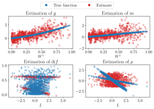
Figure S1: Estimation of nuisance functions on the simulated data in Section S3.1.1. The estimates are computed on a dataset of size $n=1000$ and the estimates (red) and true functions (blue) are evaluated on a new dataset of the same size. We see that the $m$ and $g$ estimates are reasonable estimates of the true functions, that roughly capture the behavior of the true function in an unbiased (conditioned on $W^{1}$) way. In contrast, the derivative and score estimates, are much worse at capturing the more complex behavior (with clear biases conditioned on $W^{1}$).

S3.1.2 Estimation of nuisance functions with binary $L$

To illustrate the difficulty of estimating the inverse propensity score $\pi^{-1}$ (see Section 3.2.1) compared to $m$ (in this case equal to $\pi$) and $g$ (see Section 3.2.3) we estimate the functions on simulated data and compare the estimates to the truth. We simulate $n=1000$ observations from the model where $W$ is uniformly distributed on $\Delta^{2}$, $\varepsilon$ is standard Gaussian independent of $W$, $L$ conditioned on $W$ is generated as a Bernoulli random variable with success probability $\pi(W):=0.95\mathrm{expit}(\mathrm{logit}(W^{1}))+0.05$ and

$$Y:=2LW^{1}+\varepsilon.$$

The out-of-sample predictions evaluated on new dataset with $n=1000$ observations can be seen together with the true function in Figure S2.

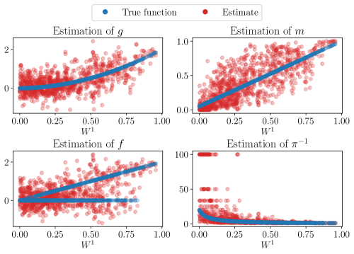
Figure S2: Estimation of nuisance functions on the simulated data in Section S3.1.2. The estimates are computed on a dataset of size $n=1000$ and the estimates (red) and true functions (blue) are evaluated on a new dataset of the same size. We see that the $m$, $g$ and $f$ estimates are reasonable estimates of the true functions whereas the inverse propensity (even when cutting off extreme values at $100$) is poorly estimated for $W^{1}$ close to zero.

S3.1.3 Partially linear model estimate when partial linearity is violated

The estimators based on the partially linear model are still well-behaved even in settings where the model is misspecified. The estimand $\mathbb{E}[\mathrm{cov}(Y,L\,|\,W)]/\mathbb{E}[\mathrm{var}(L\,|\,W)]$ just happens to be different from $\tau$ and $\lambda$ (depending on the setting). We can see this by plotting the distribution of the estimates from the $d=15$ experiment (with $Y$ nonparametric) of Section 4.1 which we do in Figure S3. Even though the estimand is different, it is still related to the original target parameters, since it can be seen as the ’best approximation’ to a generic nonparametric model, as shown in the following proposition.

Proposition S1.

Let $(Y,L,W)\in\mathbb{R}\times\mathbb{R}\times\mathcal{W}$ denote random variables where $\max\{\mathbb{E}[L^{2}],\mathbb{E}[Y^{2}]\}<\infty$. Then,

$$\theta:=\frac{\mathbb{E}[\mathrm{cov}(Y,L\,|\,W)]}{\mathbb{E}[\mathrm{var}(L\,|\,W)]}\quad\text{and}\quad h:w\mapsto\mathbb{E}[Y\,|\,W=w]-\theta\mathbb{E}[L\,|\,W=w]$$

are solutions to the minimization problem

$$\min_{\theta\in\mathbb{R},h:\mathcal{W}\to\mathbb{R}}\mathbb{E}\left[\left(\mathbb{E}[Y\,|\,L,W]-\theta L-h(W)\right)^{2}\right].$$ (S4)

Proof.

First, we note that instead of the optimization in (S4) we can also solve

$$\min_{\theta\in\mathbb{R},\widetilde{h}:\mathcal{W}\to\mathbb{R}}\underbrace{\mathbb{E}\left[\left(\mathbb{E}[Y\,|\,L,W]-\mathbb{E}[Y\,|\,W]-\theta(L-\mathbb{E}[Y\,|\,W])-\widetilde{h}(W)\right)^{2}\right]}_{=c(\theta,\widetilde{h})},$$ (S5)

since using $h:w\mapsto\widetilde{h}(w)+\mathbb{E}[Y\,|\,W=w]-\theta\mathbb{E}[L\,|\,W=w]$ leads to a solution of (S4). Next, we expand the square in the objective function of the minimization problem (S5) and obtain that

$$c(\theta,\widetilde{h}) =\mathbb{E}\left[\left(\mathbb{E}[Y\,|\,L,W]-\mathbb{E}[Y\,|\,W]\right)^{2}\right]+\theta^{2}\mathbb{E}\left[\mathrm{var}(L\,|\,W)\right]+\mathbb{E}[\widetilde{h}(W)^{2}]$$

$$-2\theta\mathbb{E}[(\mathbb{E}[Y\,|\,L,W]-\mathbb{E}[Y\,|\,W])(L-\mathbb{E}[L\,|\,W])].$$

It is now clear that the optimal $\widetilde{h}$ is the zero function and by noting that

$$\mathbb{E}[(\mathbb{E}[Y\,|\,L,W]-\mathbb{E}[Y\,|\,W])(L-\mathbb{E}[L\,|\,W])]=\mathbb{E}[\mathrm{cov}(Y,L\,|\,W)],$$

we obtain the desired result by minimizing the quadratic in $\theta$. ∎

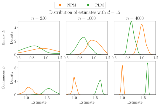
Figure S3: Smoothed empirical distributions of the estimates for the nonparametric model (NPM) and partially linear model (PLM) estimators in the nonparametric settings described in Section 4.1 with $d=15$. We see that while the NPM estimator correctly clusters around the true value of $1$, the PLM estimator also clusters however around a different, but potentially still useful, value.

S3.2 Computing directional perturbation effects in the presence of zero speeds

In Proposition 1 we only considered directional perturbations where $\omega_{\psi}(Z)\neq 0$ almost surely. We would, however, like to be able to use the derivative-isolating reparametrizations for estimation of the directional average perturbation effect $\tau_{\psi}$ even when this is not the case. To that end, we propose a modified estimation procedure that we outline in Algorithm S1. We propose to estimate $\tau_{\psi}$ on the subset of observations where $\omega_{\psi}(Z)\neq 0$ and then correct the resulting point and variance estimate appropriately.

Algorithm S1 Estimation of $\tau_{\psi}$ in the presence of observations with $\omega_{\psi}(Z)=0$.

1:Input: Data $(Y_{i},Z_{i})_{i\in[n]}$, directional perturbation $\psi$, derivative-isolating reparametrization $\phi$.

2:For $i\in[n]$, define $D_{i}:=\mathbbm{1}_{\{\omega_{\psi}(Z_{i})\neq 0\}}$.

3:Define $\mathcal{I}:=\{i\in[n]\mid D_{i}=1\}$.

4:For $i\in\mathcal{I}$, define $(L_{i},W_{i})=\phi(Z_{i})$.

5:Compute estimate $\widehat{\tau}$ and asymptotic variance estimate $\widehat{\sigma}^{2}$ from either Algorithm 1 or 3.

6:Compute $\widehat{p}:=\frac{1}{n}\sum_{i=1}^{n}D_{i}$.

7:return estimate $\widetilde{\tau}:=\widehat{\tau}\widehat{p}$ and asymptotic variance estimate $\widetilde{\sigma}^{2}:=\widehat{p}\widehat{\sigma}^{2}+\widehat{\tau}^{2}\widehat{p}(1-\widehat{p})$.

Theoretical guarantees for the proposed modification follow from repeating the arguments of the proof of Theorem 1 (a) and (c) to obtain the population quantities that determine the asymptotic behavior of $\widehat{\tau}$ and $\widehat{\sigma}^{2}$ and then applying Proposition S2 below.

Proposition S2.

Let $(D,S)\in\{0,1\}\times\mathbb{R}$ be a pair of random variables with distributions determined by $\mathcal{P}$ and let $(S_{n},D_{n})_{n\in\mathbb{N}}$ be an i.i.d. sequence of copies of $(S,D)$. Suppose that there exist $\delta,C,c>0$ such that $\mathrm{var}_{P}(DS)\geq c$ and $\mathbb{E}_{P}[D|S|^{2+\delta}]\leq C$. Suppose further that

$$\widehat{\tau}=\frac{1}{\sum_{i=1}^{n}D_{i}}\sum_{i=1}^{n}D_{i}S_{i}+o_{\mathcal{P}}(n^{-1/2})$$

and

$$\widehat{\sigma}^{2}=\frac{1}{\sum_{i=1}^{n}D_{i}}\sum_{i=1}^{n}D_{i}S_{i}^{2}-\left(\frac{1}{\sum_{i=1}^{n}D_{i}}\sum_{i=1}^{n}D_{i}S_{i}\right)^{2}+o_{\mathcal{P}}(1).$$

Then,

$$\widehat{p}:=\frac{1}{n}\sum_{i=1}^{n}D_{i},\quad\widetilde{\tau}:=\widehat{\tau}\widehat{p},\quad\text{and}\quad\widetilde{\sigma}^{2}:=\widehat{p}\widehat{\sigma}^{2}+\widehat{\tau}^{2}\widehat{p}(1-\widehat{p})$$

satisfy

$$\lim_{n\to\infty}\sup_{P\in\mathcal{P}}\sup_{x\in\mathbb{R}}\left|\mathbb{P}_{P}\left(\frac{\sqrt{n}}{\widetilde{\sigma}}(\widetilde{\tau}-\tau_{P})\leq x\right)-\Phi(x)\right|=0.$$

Proof.

We first note that

$$\widetilde{\tau}:=\frac{1}{n}\sum_{i=1}^{n}D_{i}S_{i}+o_{\mathcal{P}}(n^{-1/2})$$

since $\widehat{p}\leq 1$. Similarly, we have that

$$\widetilde{\sigma}^{2}=\frac{1}{n}\sum_{i=1}^{n}D_{i}S_{i}^{2}-\left(\frac{1}{n}\sum_{i=1}^{n}D_{i}S_{i}\right)^{2}+o_{\mathcal{P}}(1).$$

Therefore, by several applications of Lemma S2, we have that

$$\frac{\sqrt{n}}{\widetilde{\sigma}}(\widetilde{\tau}-\tau_{P})=\frac{\frac{1}{\sqrt{n}}\sum_{i=1}^{n}(D_{i}S_{i}-\tau_{P})}{\left(\frac{1}{n}\sum_{i=1}^{n}D_{i}S_{i}^{2}-\left(\frac{1}{n}\sum_{i=1}^{n}D_{i}S_{i}\right)^{2}\right)^{1/2}}+o_{\mathcal{P}}(1)$$

and the result thus follows by Lemma S4 (a) by the bounds on the moments and variance of $(D,S)$. ∎

S3.3 Estimating differentiable regression functions

The following is a description of the smoothing method we apply in the nonparametric estimator of the average directional perturbation effect. The procedure uses random forest weights together with a local polynomial estimate to smooth a given regression function to produce a differentiable estimator and to compute its derivatives. Local polynomials are a prominent and natural method used to estimate derivatives [e.g., Masry and Fan, 1997, De Brabanter et al., 2013]. We are interested in estimating the partial derivative of a function $g:\mathbb{R}\times\mathcal{W}\rightarrow\mathbb{R}$. As in Klyne and Shah [2023] we start from a given arbitrary regression estimate $\widehat{g}$ of $g$ and apply the following local polynomial approach. Estimate, for all $i\in[n]$, polynomial coefficients $\beta\in\mathbb{R}^{3}$ such that the polynomial $p:\mathbb{R}\rightarrow\mathbb{R}$ defined for all $\ell\in\mathbb{R}$ by

$$p(\ell)=\beta^{1}+\beta^{2}(\ell-L_{i})+\beta^{3}(\ell-L_{i})^{2}$$

is a good local approximation of $\widehat{g}$ around $L_{i}$. Formally, for a given weight matrix $K\in\mathbb{R}^{n\times n}$, which encodes a closeness measure between sample points, we minimize for all $i\in[n]$ the weighted mean squared loss

$$\hat{\beta}(i):=\operatorname{argmin}_{\beta\in\mathbb{R}^{3}}\sum_{k=1}^{n}\left(\widehat{g}(L_{k},W_{k})-\sum_{j=1}^{3}\beta^{j}(L_{k}-L_{i})^{j-1}\right)^{2}K_{i,\ell}.$$ (S6)

Then, using the estimated coefficients $\hat{\beta}(i)$, we get a smoothed estimate $\widehat{g}_{s}$ which at each sample point $i\in[n]$ is given by

$$\widehat{g}_{s}(L_{i},W_{i}):=\hat{\beta}^{1}(i)\quad\text{and}\quad\partial_{\ell}\widehat{g}_{s}(L_{i},W_{i}):=\hat{\beta}^{2}(i).$$ (S7)

As weights $K$ we could, for example, use kernel weights, i.e., $K_{i,\ell}=k((X_{i}-X_{\ell})/\sigma)$ for a kernel function $k$ and a bandwidth $\sigma>0$. As we are considering a potentially high-dimensional setting, we instead propose to use random forest weights [Meinshausen, 2006, Athey et al., 2019]. The full procedure is detailed in Algorithm S2.

Algorithm S2 Local polynomial based smoothing with random forest weights

1:Input: Data $(L_{i},W_{i})_{i\in[n]}$, fitted values $(\widehat{g}(L_{i},W_{i}))_{i\in[n]}$

2:Regress $(\widehat{g}(L_{i},W_{i}))_{i\in[n]}$ on $(L_{i},W_{i})_{i\in[n]}$ using a random forest yielding $\widehat{\mu}$.

3:Extract weight matrix $K$ from $\widehat{\mu}$.

4:for $i=1,\ldots,n$ do

5:     Set $\hat{\beta}(i)$ to equal the coefficient of a degree $2$ local polynomial fit in (S6).

6:     Set $\widehat{g}_{s}(L_{i},W_{i}):=\hat{\beta}^{1}(i)$.

7:     Set $\partial_{\ell}\widehat{g}_{s}(L_{i},W_{i}):=\hat{\beta}^{2}(i)$.

8:return smoothed predictions $(\widehat{g}_{s}(L_{i},W_{i}))_{i\in[n]}$ and derivatives $(\partial_{\ell}\widehat{g}_{s}(L_{i},W_{i}))_{i\in[n]}$

S3.4 Location-scale modelling of the score function

The following is a description of the estimator of the conditional score based on a location-scale model proposed by Klyne and Shah [2023]. We apply this in our experiments to estimate conditional score functions and include it here for completeness. We are interested in the estimation of the conditional score of $L$ given $W$, where $L\in\mathbb{R}$ and $W\in\mathcal{W}$, that is, the derivative of the logarithm of the conditional density of $L$ given $W$. Conditional density estimation is difficult even in low dimensions. However, if we are willing to assume that there exist functions $m:\mathcal{W}\rightarrow\mathbb{R}$, $v:\mathcal{W}\rightarrow[0,\infty)$ and a random variable $\zeta\in\mathbb{R}$ that is independent of $W$ such that

$$L=m(W)+v(W)^{1/2}\zeta,$$

we can simplify estimation of the score function. The procedure is outlined in Algorithm S3 below. In all of our experiments, we use the univariate score estimation method given by Ng [1994] that is based on ideas from Cox [1985].

Algorithm S3 Location-scale score modelling estimation

1:Input: Data $(L_{i},W_{i})_{i\in[n]}$, nuisance regression methods $\widehat{\eta}=(\widehat{m}$, $\widehat{v})$, univariate score estimator $\widehat{\rho}$.

2:Split indices $\{1,\dots,n\}$ into $2$ disjoint sets $I_{1},I_{2}$ of (roughly) equal size.

3:Regress $L$ on $W$ using $I_{1}$ yielding regression estimate $\widehat{m}$.

4:Regress $(L-\widehat{m}(w))^{2}$ on $W$ using $I_{1}$ yielding variance estimate $\widehat{v}$.

5:For $i\in I_{2}$, set $\widehat{\xi}_{i}:=\frac{L_{i}-\widehat{m}(W_{i})}{\widehat{v}(W_{i})^{1/2}}$.

6:Estimate a univariate score from $(\widehat{\xi}_{i})_{i\in I_{2}}$ yielding $\widehat{\rho}$.

7:return $\widehat{\rho}$.

Appendix S4 Details and additional results from numerical experiments

Section S4.1 provides the details behind the experiments in Table 1 in Section 1. Section S4.2 contains additional simulation results from our investigation into the performance of various semiparametric estimators. Section S4.3 provides a detailed description of how we generate the groups used for aggregation in the experiment described in Section 4.2.

S4.1 Simulations from Section 1

In this section we describe the data-generating processes and methods used in the numerical illustrations of Example 1 and Example 2. The results of are provided in Table 1.

S4.1.1 Example 1: Effects of absence or presence of microbes

Let $L\sim\mathrm{Bern}(1/2)$, $U^{W},U^{L}\sim\mathrm{Unif}([0,1])$ and $B\sim\mathrm{Bern}(1/2)$ be independent random variables and define

$$Z:=(Z^{1},W^{2}(1-Z^{1}),(1-W^{2})(1-Z^{1}))\in\Delta^{2},$$

where $W^{2}:=U^{W}(1-L)+U^{W}LB$ and $Z^{1}:=(1-L)U^{L}$. Furthermore, define $Y$ such that

$$Y\,|\,Z\sim\mathrm{Bern}\left(\frac{3}{4}-\frac{1}{8}\mathbbm{1}_{\{Z^{1}=0\}}+\frac{1}{2}\mathbbm{1}_{\{Z^{2}=0\}}\right).$$

In the experiment, we generate $n=1000$ i.i.d. copies $(Y_{1},Z_{1}),\ldots,(Y_{n},Z_{n})$ of $(Y,Z)$.

$\mathrm{CKE}^{1}$ is computed using the $\lambda$-estimator based on a partially linear model for $Y$ (Algorithm 3) with $10$-fold cross-fitting and random forests for all regressions.

S4.1.2 Example 2: Effects of increased diversity

Let $\Pi$ denote the orthogonal projection onto the orthogonal complement of $\mathrm{span}((1,1,1))$. Moreover, let $U\sim\mathcal{N}(0,\Pi\,\Pi^{\top})$ and $\xi,\varepsilon\sim\mathcal{N}(0,1)$ be independent random variables and define

$$Z:=-DW+z_{\mathrm{cen}}\in\Delta^{2}\quad\text{and}\quad Y:=L+4W^{\top}e_{1}+\varepsilon,$$

where $W:=\frac{U}{\|U\|_{1}}$, $D:=\mathrm{expit}(W^{\top}e_{1}+\xi)$ and $L:=-\frac{2}{9}D\sum_{j=1}^{3}\sum_{k=1}^{3}|W^{j}-W^{k}|$. Then, by construction $L$ is minus the Gini coefficient of $Z$. Hence, from the partially linear model of $Y$ it follows that the true effect of increasing the negative Gini coefficient is equal to $1$. In the experiment, we generate $n=1000$ i.i.d. copies $(Y_{1},Z_{1}),\ldots,(Y_{n},Z_{n})$ of $(Y,Z)$.

$\mathrm{CDI}_{\mathrm{Gini}}$ is computed using the $\tau$-estimator based on a partially linear model for $Y$ (Algorithm 3) with $10$-fold cross-fitting and random forests for all regressions.

S4.2 Additional semiparametric estimation results

Here we provide additional results from the experiment of Section 4.1. Figure S4 and Figure S5 contain estimated coverage rates of the $95\%$ confidence intervals for the different methods and settings with $d=3$ and $d=75$, respectively. The patterns observed in Figure 4 of Section 4.1 are repeated in these figures.

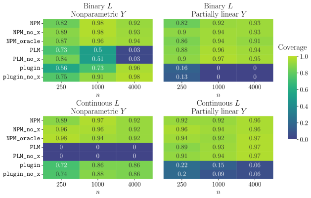
Figure S4: Estimated coverage rates of the $95\%$ confidence intervals over $100$ repetitions for each of the settings described in Section 4.1 with $d=3$. The patterns observed in Figure 4 of Section 4.1 are repeated here.

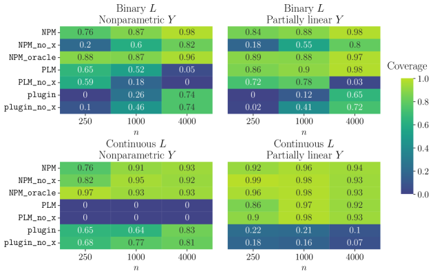
Figure S5: Estimated coverage rates of the $95\%$ confidence intervals over $100$ repetitions for each of the settings described in Section 4.1 with $d=75$. The patterns observed in Figure 4 of Section 4.1 are repeated here.

S4.3 Description of the construction of groups in Section 4.2

In this section we describe how we construct the two community-level grouped datasets analyzed in Section 4.2. On the individual-level data the observed proportions of race (categorical, ’White’, ’Black’ and ’Other’), education (binary, $1$ if strictly greater than high school and $0$ otherwise) and compensation (binary, $1$ if compensation above 50,000 USD per year and $0$ otherwise) are

$$(\widehat{\pi}_{R}(\mathrm{White}),\widehat{\pi}_{R}(\mathrm{Black}),\widehat{\pi}_{R}(\mathrm{Other})) =(0.855,0.096,0.049),$$

$$(\widehat{\pi}_{E}(0),\widehat{\pi}_{E}(1)) =(0.454,0.546),$$

$$(\widehat{\pi}_{C}(0),\widehat{\pi}_{C}(1)) =(0.761,0.239),$$

respectively. Now, for the two types of groupings we define target probabilities $p_{i}=(p_{i}^{0},p_{i}^{1},p_{i}^{2})\in\Delta^{2}$ for each individual $i$ (see below). Based on these probabilities we randomly draw for each individual $i$ one of the three categories using the probabilities $p_{i}$. Finally, we randomly group individuals with the same categories into communities of approximately $50$ (as many communities of $50$ and the remaining with $49$) and aggregate the predictors and response as described in the main text. The probabilities $(p_{i}^{0},p_{i}^{1},p_{i}^{2})\in\Delta^{2}$ are selected, in each of the two settings, as follows.

Grouping by race and education: The probability $p_{i}^{1}$ of observation $i$ belonging to category $1$ is set to

$$p_{i}^{1}:=p_{R}^{1}(\texttt{race}_{i})\cdot p_{E}^{1}(\texttt{education}_{i}),$$

where $\texttt{race}_{i}$ and $\texttt{education}_{i}$ denote the race and education level of the $i$th individual, $p_{R}^{1}$ and $p_{E}^{1}$ are probability vectors satisfying

$$p_{R}^{1}(\mathrm{White})\propto\frac{0.8}{\widehat{\pi}_{R}(\mathrm{White})},\quad p_{R}^{1}(\mathrm{Black})\propto\frac{0.02}{\widehat{\pi}_{R}(\mathrm{Black})},\quad p_{R}^{1}(\mathrm{Other})\propto\frac{0.18}{\widehat{\pi}_{R}(\mathrm{Other})},$$ (S8)

and

$$p_{E}^{1}(0)\propto\frac{0.95}{\widehat{\pi}_{E}(0)},\quad p_{E}^{1}(1)\propto\frac{0.05}{\widehat{\pi}_{E}(1)}.$$

That is, category $1$ is about as diverse ($(0.8,0.02,0.18)$ is about as diverse as $\widehat{\pi}_{R}$) and with lower education ($0.05<\widehat{\pi}_{E}(1)$). The probability $p_{i}^{2}$ of observation $i$ belonging to category $2$ is set to

$$p_{i}^{2}:=p_{R}^{2}(\texttt{race}_{i})\cdot p_{E}^{2}(\texttt{education}_{i}),$$

where similarly $p_{R}^{2}$ and $p_{E}^{2}$ are probability vectors but now satisfying

$$p_{R}^{2}(\mathrm{White})\propto\frac{0.65}{\widehat{\pi}_{R}(\mathrm{White})},\quad p_{R}^{2}(\mathrm{Black})\propto\frac{0.12}{\widehat{\pi}_{R}(\mathrm{Black})},\quad p_{R}^{2}(\mathrm{Other})\propto\frac{0.23}{\widehat{\pi}_{R}(\mathrm{Other})}$$ (S9)

and

$$p_{E}^{2}(0)\propto\frac{0.3}{\widehat{\pi}_{E}(0)},\quad p_{E}^{2}(1)\propto\frac{0.7}{\widehat{\pi}_{E}(1)}.$$

That is, category $2$ is more diverse ($(0.65,0.12,0.23)$ is more diverse than $\widehat{\pi}_{R}$) and with higher education ($0.7>\widehat{\pi}_{E}(1)$). Lastly, the probability $p_{i}^{0}$ for category $0$ is set to $p_{i}^{0}:=1-p_{i}^{1}-p_{i}^{2}$.

Grouping by race and compensation: The probability $p_{i}^{1}$ of observation $i$ belonging to category $1$ is set to

$$p_{i}^{1}:=p_{R}^{1}(\texttt{race}_{i})\cdot p_{C}^{1}(\texttt{compensation}_{i}),$$

where $p_{R}^{1}$ is as in (S8) and $p_{C}^{1}$ is a probability vector satisfying

$$p_{C}^{1}(0)\propto\frac{0.9}{\widehat{\pi}_{C}(0)},\quad p_{C}^{1}(1)\propto\frac{0.1}{\widehat{\pi}_{C}(1)}.$$

That is, category $1$ is about as diverse and with lower compensation ($0.05<\widehat{\pi}_{C}(1)$). The probability $p_{i}^{2}$ for category $2$ is set to

$$p_{i}^{2}:=p_{R}^{2}(\texttt{race}_{i})\cdot p_{C}^{2}(\texttt{compensation}_{i}),$$

where $p_{R}^{2}$ is as in (S9) and $p_{C}^{2}$ is a probability vector satisfying

$$p_{C}^{2}(0)\propto\frac{0.7}{\widehat{\pi}_{C}(0)},\quad p_{C}^{2}(1)\propto\frac{0.3}{\widehat{\pi}_{C}(1)}.$$

That is, category $2$ is more diverse and with higher compensation ($0.3>\widehat{\pi}_{C}(1)$). Lastly, we set the probability $p_{i}^{0}$ for category $0$ is $p_{i}^{0}:=1-p_{i}^{1}-p_{i}^{2}$.

S4.4 Additional plots from gut microbiome analysis in Section 4.3

In this section we provide an additional figure showing our results from the analysis of the gut microbiome data in Section 4.3. In Figure S6, we plot the most significant hits for $\mathrm{CFI}{\mathrm{unit}}$ and $\mathrm{CKE}$ both estimated using random forests together with $\mathrm{CFI}_{\mathrm{mult}}$ estimates. We plot the estimates scaled by the estimated standard deviation of $L$ to put the effects on the same scale (we do not correct the confidence intervals for the estimation of this standard deviation). Furthermore, we flip the sign of $\mathrm{CKE}$ to keep the interpretation similar to $\mathrm{CFI}$, that is, that we are looking at the effect of increasing $Z^{j}$.

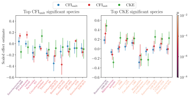
Figure S6: Effect estimates scaled by the estimated standard deviation of $L$ for the $10$ most significant (smallest $p$-value) species from $\mathrm{CFI}_{\mathrm{unit}}$ (left) and $\mathrm{CKE}$ (right). The labels are colored by the size of the $p$-value. For the $\mathrm{CFI}_{\mathrm{unit}}$ results, the first $9$ species remain below $0.05$ after Bonferroni-correction while this is only true for $2$ for the $\mathrm{CKE}$. There is little overlap between the selected species across the two methods.

Appendix S5 Proof of Theorem 1

S5.1 Proof of (a)

Proof.

We define for all $k\in[K]$ and $r\in\{0,1\}$, $N_{k,r}:=|I_{k,r}|$ and for all $i\in[n]$, $\varepsilon_{i}:=Y_{i}-f(L_{i},W_{i})$. We first argue that

$$\widehat{\tau}=\frac{1}{n}\sum_{i=1}^{n}\underbrace{\partial_{\ell}f_{P}(L_{i},W_{i})-\rho_{P}(L_{i},W_{i})\varepsilon_{i}}_{S_{i}}+o_{\mathcal{P}}(n^{-1/2}).$$ (S10)

To that end, we write for all $k\in[K]$ and $r\in\{0,1\}$

$$\widehat{\tau}_{k,r} =\frac{1}{N_{k,r}}\sum_{i\in I_{k,r}}S_{i}$$

$$+\underbrace{\frac{1}{N_{k,r}}\sum_{i\in I_{k,r}}\{\widehat{\rho}_{k,r}(L_{i},W_{i})-\rho_{P}(L_{i},W_{i})\}\{\widehat{f}_{k}(L_{i},W_{i})-f_{P}(L_{i},W_{i})\}}_{(\textup{I})}$$

$$-\underbrace{\frac{1}{N_{k,r}}\sum_{i\in I_{k,r}}\{\widehat{\rho}_{k,r}(L_{i},W_{i})-\rho_{P}(L_{i},W_{i})\}\varepsilon_{i}}_{(\textup{II})}$$

$$+\underbrace{\frac{1}{N_{k,r}}\sum_{i\in I_{k,r}}\{\partial_{\ell}\widehat{f}_{k}(L_{i},W_{i})-\partial_{\ell}f_{P}(L_{i},W_{i})\}+\rho_{P}(L_{i},W_{i})\{\widehat{f}_{k}(L_{i},W_{i})-f_{P}(L_{i},W_{i})\}}_{(\textup{III})}.$$

By the Cauchy–Schwarz inequality, Assumption 1 (f) and Lemma S3, we have

$$|(\textup{I})|\leq\sqrt{\frac{1}{N_{k,r}}\sum_{i\in I_{k,r}}\{\widehat{\rho}_{k,r}(L_{i},W_{i})-\rho_{P}(L_{i},W_{i})\}^{2}\frac{1}{N_{k,r}}\sum_{i\in I_{k,r}}\{\widehat{f}_{k}(L_{i},W_{i})-f_{P}(L_{i},W_{i})\}^{2}}=o_{\mathcal{P}}(n^{-1}).$$

Since the summands of $(\textup{II})$ are conditionally i.i.d. and mean zero given $(L_{i},W_{i})_{i\in I_{k,r}}$ and $\widehat{\rho}_{k,r}$, we have by conditional Chebyshev’s inequality that for any $\epsilon>0$

$$\mathbb{P}_{P}(|(\textup{II})|\geq N_{k,r}^{-1/2}\epsilon\,|\,(L_{i},W_{i})_{i\in I_{k,r}},\widehat{\rho}_{k,r})\leq\frac{1}{N_{k}\epsilon^{2}}\sum_{i\in I_{k,r}}\{\widehat{\rho}_{k,r}(L_{i},W_{i})-\rho_{P}(L_{i},W_{i})\}^{2}\mathrm{var}_{P}(Y_{i}\,|\,L_{i},W_{i}).$$

Combining the above with Assumption 1 (a) and (e), we have

$$\mathbb{P}_{P}(|(\textup{II})|\geq N_{k,r}^{-1/2}\epsilon\,|\,(L_{i},W_{i})_{i\in I_{k,r}},\widehat{\rho}_{k,r})=o_{\mathcal{P}}(1)$$

which implies $(\textup{II})=o_{\mathcal{P}}(N_{k}^{-1/2})$ as $\epsilon$ was arbitrary.

To deal with the $(\textup{III})$ term, let $i\in I_{k,r}$ be fixed and note that by the triangle inequality, the Cauchy–Schwarz inequality for conditional expectations and independence of $(L_{i},W_{i})$ from $\widehat{f}_{k}$, we have

$$\mathbb{E}_{P}\left[\left|\partial_{\ell}\widehat{f}_{k}(L_{i},W_{i})-\partial_{\ell}f_{P}(L_{i},W_{i})+\rho_{P}(L_{i},W_{i})\{\widehat{f}_{k}(L_{i},W_{i})-f_{P}(L_{i},W_{i})\}\right|\,|\,\widehat{f}_{k}\right]$$

$$\leq\mathbb{E}_{P}[|\partial_{\ell}\widehat{f}_{k}(L_{i},W_{i})-\partial_{\ell}f_{P}(L_{i},W_{i})|\,|\,\widehat{f}_{k}]+\mathbb{E}_{P}\left[\rho_{P}(L_{i},W_{i})^{2}\right]^{1/2}\mathbb{E}_{P}\left[\{\widehat{f}_{k}(L_{i},W_{i})-f_{P}(L_{i},W_{i})\}^{2}\,|\,\widehat{f}_{k}\right]^{1/2}.$$

By the above, Assumption 1 (c), (d) and (a), Lemma S2 (a) and Jensen’s inequality, we have that

$$\mathbb{E}_{P}\left[\left|\partial_{\ell}\widehat{f}_{k}(L_{i},W_{i})-\partial_{\ell}f_{P}(L_{i},W_{i})+\rho_{P}(L_{i},W_{i})\{\widehat{f}_{k}(L_{i},W_{i})-f_{P}(L_{i},W_{i})\}\right|\,|\,\widehat{f}_{k}\right] =O_{\mathcal{P}}(1),$$

$$\mathbb{E}_{P}\left[\left|\widehat{f}_{k}(L_{i},W_{i})-f_{P}(L_{i},W_{i})\right|\,|\,\widehat{f}_{k}\right] =O_{\mathcal{P}}(1).$$

This implies that for any $\zeta>0$, we can find $M>0$ and $n\in\mathbb{N}$ so that

$$\Omega_{P} :=\left\{\mathbb{E}_{P}\left[\left|\widehat{f}_{k}(L_{i},W_{i})-f_{P}(L_{i},W_{i})\right|\,|\,\widehat{f}_{k}\right]<M\right\}$$

$$\cap\left\{\mathbb{E}_{P}\left[\left|\partial_{\ell}\widehat{f}_{k}(L_{i},W_{i})-\partial_{\ell}f_{P}(L_{i},W_{i})+\rho_{P}(L_{i},W_{i})\{\widehat{f}_{k}(L_{i},W_{i})-f_{P}(L_{i},W_{i})\}\right|\,|\,\widehat{f}_{k}\right]<M\right\}$$

satisfies $\mathbb{P}_{P}(\Omega_{P})\geq 1-\zeta/2$ for all $P\in\mathcal{P}$. We therefore have for any $\epsilon>0$

$$\sup_{P\in\mathcal{P}}\mathbb{P}_{P}(|(\textup{III})|\geq N_{k,r}^{-1/2}\epsilon)\leq\sup_{P\in\mathcal{P}}\mathbb{P}_{P}(\{|(\textup{III})|\geq N_{k,r}^{-1/2}\epsilon\}\cap\Omega_{P})+\zeta/2\leq\sup_{P\in\mathcal{P}}\mathbb{P}_{P}(|\mathbbm{1}_{\Omega_{P}}\cdot(\textup{III})|\geq N_{k,r}^{-1/2}\epsilon)+\zeta/2,$$

hence it suffices to prove that $\mathbbm{1}_{\Omega_{P}}\cdot(\textup{III})=o_{\mathcal{P}}(N_{k,r}^{-1/2})$ to conclude that $(\textup{III})=o_{\mathcal{P}}(N_{k,r}^{-1/2})$. To that end, we first note that

$$\mathbb{E}_{P}\left[\mathbbm{1}_{\Omega_{P}}\cdot(\textup{III})\,|\,\widehat{f}_{k}\right]=\mathbb{E}_{P}\left[\mathbbm{1}_{\Omega_{P}}\left(\partial_{\ell}\widehat{f}_{k}(L_{i},W_{i})-\partial_{\ell}f_{P}(L_{i},W_{i})+\rho_{P}(L_{i},W_{i})\{\widehat{f}_{k}(L_{i},W_{i})-f_{P}(L_{i},W_{i})\}\right)\,|\,\widehat{f}_{k}\right].$$

We will show that

$$\mathbb{E}_{P}\left[\mathbbm{1}_{\Omega_{P}}\cdot(\textup{III})\,|\,\widehat{f}_{k}=h\right]=0$$ (S11)

for $\mathbb{P}_{P}$-almost every $h$. If $h$ is such that $\mathbbm{1}_{\Omega_{P}}=0$ then clearly the conditional expectation is $0$. If $h$ is such that $\mathbbm{1}_{\Omega_{P}}=1$, then we intend to apply Lemma S5 (integration by parts) with $g=(h-f_{P})$. Assumptions (a)-(c) of Lemma S5 are clear from the above and (d) follows from Lemma S6 and Assumption (a). We conclude that

$$\mathbb{E}_{P}\left[\partial_{\ell}(h(L,W)-f_{P}(L,W))+\rho_{P}(L,W)(h(L,W)-f_{P}(L,W))\right]=0,$$

and hence (S11) is satisfied. By conditional Chebyshev’s inequality (applicable since we have shown that summands are conditionally mean zero in (S11)), the fact that $(a+b)^{2}\leq 2a^{2}+2b^{2}$ and conditional Cauchy–Schwarz inequality, we therefore have

$$\mathbb{P}_{P}(|\mathbbm{1}_{\Omega_{P}}\cdot(\textup{III})|\geq N_{k,r}^{-1/2}\epsilon\,|\,\widehat{f}_{k})$$

$$\qquad\leq\frac{1}{\epsilon^{2}N_{k,r}}\mathbb{E}_{P}[\mathbbm{1}_{\Omega_{P}}\cdot(\textup{III})^{2}\,|\,\widehat{f}_{k}]$$

$$\qquad=\frac{1}{\epsilon^{2}}\mathbb{E}_{P}\left[\left(\partial_{\ell}\widehat{f}_{k}(L_{i},W_{i})-\partial_{\ell}f_{P}(L_{i},W_{i})+\rho_{P}(L_{i},W_{i})\{\widehat{f}_{k}(L_{i},W_{i})-f_{P}(L_{i},W_{i})\}\right)^{2}\,|\,\widehat{f}_{k}\right]$$

$$\qquad\leq\frac{2}{\epsilon^{2}}\mathbb{E}_{P}\left[\left(\partial_{\ell}\widehat{f}_{k}(L_{i},W_{i})-\partial_{\ell}f_{P}(L_{i},W_{i})\right)^{2}\,|\,\widehat{f}_{k}\right]$$

$$\qquad+\frac{2}{\epsilon^{2}}\mathbb{E}_{P}\left[|\rho_{P}(L_{i},W_{i})|^{4}\right]^{1/2}\mathbb{E}_{P}\left[\left|\widehat{f}_{k}(L_{i},W_{i})-f_{P}(L_{i},W_{i})\right|^{4}\,|\,\widehat{f}_{k}\right]^{1/2}.$$

Assumption 1 (c), (d) and (a) and Lemma S3 thus yield that

$$\mathbb{P}_{P}(|\mathbbm{1}_{\Omega_{P}}\cdot(\textup{III})|\geq N_{k,r}^{-1/2}\,|\,\widehat{f}_{k})=o_{\mathcal{P}}(1)$$

which implies that $\mathbbm{1}_{\Omega_{P}}\cdot(\textup{III})=o_{\mathcal{P}}(N_{k,r}^{-1/2})$ so $(\textup{III})=o_{\mathcal{P}}(N_{k,r}^{-1/2})$ by our earlier argument. The above combined with Lemma S1 proves (S10).

Let $\delta^{\prime}:=\delta/2$. We now prove that for all $i\in[n]$ and $P\in\mathcal{P}$, we have

$$\mathbb{E}_{P}\left[|S_{i}|^{2+\delta^{\prime}}\right]\leq 2^{1+\delta^{\prime}}\left(C^{(2+\delta^{\prime})/(2+\delta)}+C2^{2+\delta^{\prime}}\right)=:C^{\prime}.$$ (S12)

By using that $|a+b|^{1+\delta}\leq 2^{\delta}(|a|^{2+\delta}+|b|^{2+\delta})$ for $\delta>0$ (sometimes known as the $c_{r}$-inequality), we have

$$|S_{i}|^{2+\delta^{\prime}}\leq 2^{1+\delta^{\prime}}\left(\left|\partial_{\ell}f_{P}(L_{i},W_{i})\right|^{2+\delta^{\prime}}+\left|\rho_{P}(L_{i},W_{i})\right|^{2+\delta}\left|\varepsilon_{i}\right|^{2+\delta}\right),$$

and

$$|\varepsilon_{i}|^{4+\delta}\leq 2^{3+\delta}\left(|Y_{i}|^{4+\delta}+|\mathbb{E}_{P}[Y_{i}\,|\,L_{i},W_{i}]|^{4+\delta}\right).$$

Therefore, using Assumption 1 (a), the Cauchy–Schwarz inequality and Jensen’s inequality, we have

$$\mathbb{E}_{P}\left[|S_{i}|^{2+\delta^{\prime}}\right] \leq 2^{1+\delta^{\prime}}\left(C^{(2+\delta^{\prime})/(2+\delta)}+\left(\mathbb{E}_{P}\left[\left|\rho_{P}(L_{i},W_{i})\right|^{4+\delta}\right]\mathbb{E}_{P}\left[\left|\varepsilon_{i}\right|^{4+\delta}\right]\right)^{1/2}\right)$$

$$\leq 2^{1+\delta^{\prime}}\left(C^{(2+\delta^{\prime})/(2+\delta)}+\left(C^{2}(2^{4+\delta})\right)^{1/2}\right)=C^{\prime}$$

as desired.

We now show that

$$\widehat{\sigma}^{2}_{\tau}=\frac{1}{n}\sum_{i=1}^{n}S_{i}^{2}-\left(\frac{1}{n}\sum_{i=1}^{n}S_{i}\right)^{2}+o_{\mathcal{P}}(1).$$ (S13)

Note that $\frac{1}{n}\sum_{i=1}^{n}S_{i}=O_{\mathcal{P}}(1)$ by (S12) and Markov’s inequality, hence by (S10) and Lemma S3, we have that

$$\widehat{\tau}^{2}=\left(\frac{1}{n}\sum_{i=1}^{n}S_{i}\right)^{2}+o_{\mathcal{P}}(1).$$

We have thus shown (S13) if we can show that

$$\frac{1}{2K}\sum_{k=1}^{K}\sum_{r=0}^{1}\widehat{\nu}_{k,r}=\frac{1}{n}\sum_{i=1}^{n}S_{i}^{2}+o_{\mathcal{P}}(1).$$

To that end using the same decomposition as for $\widehat{\tau}_{k,r}$, we write for $k\in[K]$, $r\in\{0,1\}$, $i\in I_{k,r}$

$$\partial_{\ell}\widehat{f}_{k}(L_{i},W_{i})-\widehat{\rho}_{k,r}(L_{i},W_{i})\{Y_{i}-\widehat{f}_{k,r}(L_{i},W_{i})\}=\underbrace{\partial_{\ell}f_{P}(L_{i},W_{i})-\rho_{P}(L_{i},W_{i})\varepsilon_{i}}_{S_{i}}$$

$$\underbrace{\boxed{\begin{aligned} &+\{\widehat{\rho}_{k,r}(L_{i},W_{i})-\rho_{P}(L_{i},W_{i})\}\{\widehat{f}_{k}(L_{i},W_{i})-f_{P}(L_{i},W_{i})\}-\{\widehat{\rho}_{k,r}(L_{i},W_{i})-\rho_{P}(L_{i},W_{i})\}\varepsilon_{i}\\ &+\{\partial_{\ell}\widehat{f}_{k}(L_{i},W_{i})-\partial_{\ell}f_{P}(L_{i},W_{i})\}+\rho_{P}(L_{i},W_{i})\{\widehat{f}_{k}(L_{i},W_{i})-f_{P}(L_{i},W_{i})\}\end{aligned}}}_{R_{i}}$$

so that

$$\widehat{\nu}_{k,r}=\frac{1}{N_{k,r}}\sum_{i\in I_{k,r}}S_{i}^{2}+\frac{1}{N_{k,r}}\sum_{i\in I_{k,r}}R_{i}^{2}+\frac{2}{N_{k,r}}\sum_{i\in I_{k,r}}S_{i}R_{i}$$

Since $(a+b+c)^{2}\leq 3(a^{2}+b^{2}+c^{2})$ (which can be seen by the Cauchy–Schwarz inequality), we have

$$\frac{1}{N_{k,r}}\sum_{i\in I_{k,r}}R_{i}^{2} \leq 3\biggl{(}\underbrace{\frac{1}{N_{k,r}}\sum_{i\in I_{k,r}}\{\widehat{\rho}_{k,r}(L_{i},W_{i})-\rho_{P}(L_{i},W_{i})\}^{2}\{\widehat{f}_{k}(L_{i},W_{i})-f_{P}(L_{i},W_{i})\}^{2}}_{\widetilde{(\textup{I})}}$$

$$+\underbrace{\frac{1}{N_{k,r}}\sum_{i\in I_{k,r}}\{\widehat{\rho}_{k,r}(L_{i},W_{i})-\rho_{P}(L_{i},W_{i})\}^{2}\varepsilon_{i}^{2}}_{\widetilde{(\textup{II})}}$$

$$+\underbrace{\frac{1}{N_{k,r}}\sum_{i\in I_{k,r}}\left(\{\partial_{\ell}\widehat{f}_{k}(L_{i},W_{i})-\partial_{\ell}f_{P}(L_{i},W_{i})\}+\rho_{P}(L_{i},W_{i})\{\widehat{f}_{k}(L_{i},W_{i})-f_{P}(L_{i},W_{i})\}\right)^{2}}_{\widetilde{(\textup{III})}}\biggr{)}.$$

By using that $\sum_{i}a_{i}^{2}b_{i}^{2}\leq\left(\sum_{i}a_{i}^{2}\right)\left(\sum_{i}b_{i}^{2}\right)$, we have

$$\widetilde{(\textup{I})}\leq\left(\frac{1}{N_{k,r}}\sum_{i\in I_{k,r}}\{\widehat{\rho}_{k,r}(L_{i},W_{i})-\rho_{P}(L_{i},W_{i})\}^{2}\right)\left(\frac{1}{N_{k}}\sum_{i\in I_{k,r}}\left(\widehat{f}_{k}(L_{i},W_{i})-f_{P}(L_{i},W_{i})\right)^{2}\right).$$

We have already shown above as part of the argument for the $(\textup{I})$ term that the upper bound is $o_{\mathcal{P}}(1)$. Similarly, each of the remaining two terms have already been shown to be $o_{\mathcal{P}}(1)$ as part of the bounds above for the corresponding terms without tildes hence we deduce that

$$\frac{1}{N_{k,r}}\sum_{i\in I_{k,r}}R_{i}^{2}=o_{\mathcal{P}}(1).$$

By the Cauchy–Schwarz inequality, we have that

$$\frac{2}{N_{k,r}}\left|\sum_{i\in I_{k,r}}S_{i}R_{i}\right|\leq 2\left(\frac{1}{N_{k,r}^{2}}\sum_{i\in I_{k,r}}R_{i}^{2}\sum_{i\in I_{k,r}}S_{i}^{2}\right)^{1/2}.$$

Since $1/N_{k,r}\sum_{i\in I_{k,r}}S_{i}^{2}=O_{\mathcal{P}}(1)$ by (S12) and Markov’s inequality and $\frac{1}{N_{k,r}}\sum_{i\in I_{k,r}}R_{i}^{2}=o_{\mathcal{P}}(1)$ by the above, we conclude by Lemma S3 that

$$\frac{2}{N_{k,r}}\sum_{i\in I_{k,r}}S_{i}R_{i}=o_{\mathcal{P}}(1)$$

and Lemma S1 concludes the proof of (S13).

Since for all $i\in[n]$,

$$\mathbb{E}_{P}[S_{i}]=\mathbb{E}_{P}[\partial_{\ell}f_{P}(L_{i},W_{i})-\rho_{P}(L_{i},W_{i})\varepsilon_{i}]=\tau_{P},$$

and (S12) implies that $\frac{1}{\sqrt{n}}\sum_{i=1}^{n}(S_{i}-\mathrm{CFI}^{j})=O_{\mathcal{P}}(1)$, we have by Lemma S3, (S10) and (S13) that

$$\frac{\sqrt{n}}{\widehat{\sigma}_{\tau}}(\widehat{\tau}-\tau_{P})=\frac{\frac{1}{\sqrt{n}}\sum_{i=1}^{n}(S_{i}-\tau_{P})}{\left(\frac{1}{n}\sum_{i=1}^{n}S_{i}^{2}-\left(\frac{1}{n}\sum_{i=1}^{n}S_{i}\right)^{2}\right)^{1/2}}+o_{\mathcal{P}}(1).$$

The conclusion now follows from a uniform version of Slutsky’s theorem [Shah and Peters, 2020, Lemma 20] and Lemma S4 (a), which we can apply by Assumption 1 (a) and (b), since

$$\mathrm{var}_{P}(S_{i}) =\mathbb{E}_{P}\left[\left(\partial_{\ell}\widehat{f}(L,W)-\rho_{P}(L,W)(Y-f_{P}(L,W))\right)^{2}\right]-\mathbb{E}_{P}\left[\left(\partial_{\ell}\widehat{f}(L,W)\right)^{2}\right]$$

$$=\mathbb{E}_{P}[\rho_{P}(L,W)^{2}(Y-f_{P}(L,W))^{2}]=\mathbb{E}_{P}[\rho_{P}(L,W)^{2}\mathrm{var}_{P}(Y\,|\,L,W)]\geq c^{2}.$$

∎

S5.2 Proof of (b)

Proof.

We define for all $k\in[K]$, $N_{k}:=|I_{k}|$ and for all $i\in[n]$ $\varepsilon_{i}:=Y_{i}-f_{P}(L_{i},W_{i})$. We first argue that

$$\widehat{\kappa}=\frac{1}{n}\sum_{i=1}^{n}\underbrace{f_{P}(1,W_{i})-Y_{i}+\frac{\varepsilon_{i}}{\pi_{P}(W_{i})}L_{i}}_{S_{i}}+o_{\mathcal{P}}(n^{-1/2}).$$ (S14)

To that end, we write for $k\in[K]$

$$\widehat{\kappa}_{k} =\frac{1}{N_{k}}\sum_{i\in I_{k}}S_{i}$$

$$-\underbrace{\frac{1}{N_{k}}\sum_{i\in I_{k}}\left(\frac{1}{\widehat{\pi}_{k}(W_{i})}-\frac{1}{\pi_{P}(W_{i})}\right)\left(\widehat{f}_{k}(L_{i},W_{i})-f_{P}(L_{i},W_{i})\right)L_{i}}_{(\textup{I})}$$

$$+\underbrace{\frac{1}{N_{k}}\sum_{i\in I_{k}}\left(\frac{1}{\widehat{\pi}_{k}(W_{i})}-\frac{1}{\pi_{P}(W_{i})}\right)\varepsilon_{i}L_{i}}_{(\textup{II})}$$

$$+\underbrace{\frac{1}{N_{k}}\sum_{i\in I_{k}}\left(\widehat{f}_{k}(1,W_{i})-f_{P}(1,W_{i})\right)\left(1-\frac{L_{i}}{\pi_{P}(W_{i})}\right)}_{(\textup{III})}.$$

Applying the triangle and Cauchy–Schwarz inequality, followed by Assumption 2 (b) and (e) leads to

$$|(\textup{I})| \leq\sqrt{\frac{1}{N_{k}^{2}}\sum_{i\in I_{k}}\frac{\{\pi_{P}(W_{i})-\widehat{\pi}_{k}(W_{i})\}^{2}}{\widehat{\pi}_{k}(W_{i})^{2}\pi_{P}(W_{i})^{2}}\sum_{i\in I_{k}}\{\widehat{f}(L_{i},W_{i})-f_{P}(L_{i},W_{i})\}^{2}}$$

$$\leq\frac{1}{\zeta^{2}}\sqrt{\frac{1}{N_{k}^{2}}\sum_{i\in I_{k}}\{\pi_{P}(W_{i})-\widehat{\pi}_{k}(W_{i})\}^{2}\sum_{i\in I_{k}}\{\widehat{f}(L_{i},W_{i})-f_{P}(L_{i},W_{i})\}^{2}}=o_{\mathcal{P}}(N_{k}^{-1/2}).$$

Since the summands of $(\textup{II})$ are conditionally i.i.d. and mean zero given $(L_{i},W_{i})_{i\in I_{k}}$ and $\widehat{\pi}_{k}$, we have by conditional Chebyshev’s inequality that for any $\epsilon>0$

$$\mathbb{P}_{P}(|(\textup{II})|\geq N_{k}^{-1/2}\epsilon\,|\,(L_{i},W_{i})_{i\in I_{k}},\widehat{\pi}_{k}) \leq\frac{1}{N_{k}\epsilon^{2}}\sum_{i\in I_{k}}\left(\frac{1}{\widehat{\pi}_{k}(W_{i})}-\frac{1}{\pi_{P}(W_{i})}\right)^{2}\mathrm{var}_{P}(Y_{i}\,|\,W_{i},L_{i})$$

$$=\frac{1}{N_{k}\epsilon^{2}}\sum_{i\in I_{k}}\frac{\{\pi_{P}(W_{i})-\widehat{\pi}_{k}(W_{i})\}^{2}}{\widehat{\pi}_{k}(W_{i})^{2}\pi_{P}(W_{i})^{2}}\mathrm{var}_{P}(Y_{i}\,|\,W_{i},L_{i}).$$

Combining Assumption 2 (b), (c) and (a), we conclude that

$$\mathbb{P}_{P}(|(\textup{II})|\geq N_{k}^{-1/2}\epsilon\,|\,(L_{i},W_{i})_{i\in I_{k}},\widehat{\pi}_{k})=o_{\mathcal{P}}(1)$$

which implies that $(\textup{II})=o_{\mathcal{P}}(N_{k}^{-1/2})$ as $\epsilon$ was arbitrary.

The summands of $(\textup{III})$ are conditionally i.i.d. and mean zero given $(W_{i})_{i\in I_{k}}$ and $\widehat{f}_{k}$, hence by a similar argument as for the previous term, for any $\epsilon>0$,

$$\mathbb{P}(|(\textup{III})|\geq N_{k}^{-1/2}\epsilon\,|\,(W_{i})_{i\in I_{k}},\widehat{f}_{k}) \leq\frac{1}{N_{k}\epsilon^{2}}\sum_{i\in I_{k}}\mathbb{E}_{P}\left[\left(1-\frac{L_{i}}{\pi_{P}(W_{i})}\right)^{2}\,\Bigm{|}\,W_{i}\right]\left(\widehat{f}_{k}(1,W_{i})-f_{P}(1,W_{i})\right)^{2}.$$

By Assumption 2 (b), we have

$$\mathbb{E}_{P}\left[\left(1-\frac{L_{i}}{\pi_{P}(W_{i})}\right)^{2}\,\Bigm{|}\,W_{i}\right]=\frac{1}{\pi_{P}(W_{i})}-1\leq\frac{1-c}{c},$$

hence, by Assumption 2 (d),

$$\mathbb{P}_{P}(|(\textup{III})|\geq N_{k}^{-1/2}\epsilon\,|\,(W_{i})_{i\in I_{k}},\widehat{f}_{k})=o_{\mathcal{P}}(1)$$

which implies that $(\textup{III})=o_{\mathcal{P}}(N_{k}^{-1/2})$ as $\epsilon$ was arbitrary. The above combined with Lemma S1 proves (S14).

We now prove that for $i\in[n]$

$$\mathbb{E}_{P}\left[|S_{i}|^{2+\delta}\right]\leq 3^{1+\delta}C\left(1+c^{-(2+\delta)}(1+2^{2+\delta})\right)=:C^{\prime}.$$ (S15)

We have by repeated applications of Jensen’s inequality that

$$|S_{i}|^{2+\delta}\leq 3^{1+\delta}\left(|f_{P}(1,W_{i})|^{2+\delta}+|Y_{i}|^{2+\delta}+\frac{|\varepsilon_{i}|^{2+\delta}}{\pi_{P}(W_{i})^{2+\delta}}\right),$$

by Assumption 2 (b),

$$|f_{P}(1,W_{i})|^{2+\delta}=\frac{|\mathbb{E}_{P}[Y_{i}\mathbbm{1}_{\{L_{i}=1\}}\,|\,W_{i}]|^{2+\delta}}{\pi_{P}(W_{i})^{2+\delta}}\leq\mathbb{E}_{P}\left[|Y_{i}|^{2+\delta}\,|\,W_{i}\right]c^{-(2+\delta)}$$

and

$$|\varepsilon_{i}|^{2+\delta}\leq 2^{1+\delta}\left(|Y_{i}|^{2+\delta}+|\mathbb{E}_{P}[Y_{i}\,|\,W_{i},L_{i}]|^{2+\delta}\right).$$

Therefore, using Assumption 2 (a)

$$\mathbb{E}_{P}\left[|S_{i}|^{2+\delta}\right]\leq 3^{1+\delta}\mathbb{E}_{P}\left[|Y_{i}|^{2+\delta}\right]\left(1+c^{-(2+\delta)}(1+2^{1+\delta})\right)\leq C^{\prime}$$

as desired.

Define $\kappa_{P}:=\mathbb{E}_{P}[S_{i}]$ and $\sigma^{2}_{\kappa_{P}}:=\mathrm{var}_{P}(S_{i})$. We now show that

$$\frac{1}{K}\sum_{j=1}^{k}\widehat{\nu}_{k}-\widehat{\kappa}^{2}=\sigma^{2}_{\kappa_{P}}+o_{\mathcal{P}}(1).$$ (S16)

By (S14) and Chebyshev’s inequality, we have that

$$\widehat{\kappa}=\kappa_{P}+o_{\mathcal{P}}(1),$$

thus by (S15) and Lemma S3, we have

$$\widehat{\kappa}^{2}=\kappa_{P}^{2}+o_{\mathcal{P}}(1).$$

We have therefore shown (S16) if we can show that

$$\frac{1}{K}\sum_{k=1}^{K}\widehat{\nu}_{k}=\mathbb{E}_{P}[S_{i}^{2}]+o_{\mathcal{P}}(1).$$ (S17)

To that end using the same composition as for $\widehat{\kappa}_{k}$, we write for $k\in[K]$, $i\in I_{k}$

$$\widehat{f}_{k}(1,W_{i})-Y_{i}+\frac{Y_{i}-\widehat{f}_{k}(L_{i},W_{i})}{\widehat{\pi}_{k}(W_{i})}L_{i}=\underbrace{f_{P}(1,W_{i})-Y_{i}+\frac{\varepsilon_{i}}{\pi_{P}(W_{i})}L_{i}}_{S_{i}}$$

$$\underbrace{\boxed{\begin{aligned} &-\left(\frac{1}{\widehat{\pi}_{k}(W_{i})}-\frac{1}{\pi_{P}(W_{i})}\right)\left(\widehat{f}_{k}(L_{i},W_{i})-f_{P}(L_{i},W_{i})\right)L_{i}+\left(\frac{1}{\widehat{\pi}_{k}(W_{i})}-\frac{1}{\pi_{P}(W_{i})}\right)\varepsilon_{i}L_{i}\\ &+\left(\widehat{f}_{k}(1,W_{i})-f_{P}(1,W_{i})\right)\left(1-\frac{L_{i}}{\pi_{P}(W_{i})}\right)\end{aligned}}}_{R_{i}}$$

so that

$$\widehat{\nu}_{k}=\frac{1}{N_{k}}\sum_{i\in I_{k}}S_{i}^{2}+\frac{1}{N_{k}}\sum_{i\in I_{k}}R_{i}^{2}+\frac{2}{N_{k}}\sum_{i\in I_{k}}S_{i}R_{i}.$$

We have

$$\frac{1}{N_{k}}\sum_{i\in I_{k}}R_{i}^{2} \leq 3\biggl{(}\underbrace{\frac{1}{N_{k}}\sum_{i\in I_{k}}\left(\frac{1}{\widehat{\pi}_{k}(W_{i})}-\frac{1}{\pi_{P}(W_{i})}\right)^{2}\left(\widehat{f}_{k}(L_{i},W_{i})-f_{P}(L_{i},W_{i})\right)^{2}}_{\widetilde{(\textup{I})}}$$

$$+\underbrace{\frac{1}{N_{k}}\sum_{i\in I_{k}}\left(\frac{1}{\widehat{\pi}_{k}(W_{i})}-\frac{1}{\pi_{P}(W_{i})}\right)^{2}\varepsilon_{i}^{2}}_{\widetilde{(\textup{II})}}+\underbrace{\frac{1}{N_{k}}\sum_{i\in I_{k}}\left(1-\frac{L_{i}}{\pi_{P}(W_{i})}\right)^{2}\left(\widehat{f}_{k}(1,W_{i})-f_{P}(1,W_{i})\right)^{2}}_{\widetilde{(\textup{III})}}\biggr{)}.$$

By using that $\sum_{i}a_{i}^{2}b_{i}^{2}\leq\left(\sum_{i}a_{i}^{2}\right)\left(\sum_{i}b_{i}^{2}\right)$, we have

$$\widetilde{(\textup{I})}\leq\left(\frac{1}{N_{k}}\sum_{i\in I_{k}}\left(\frac{1}{\widehat{\pi}_{k}(W_{i})}-\frac{1}{\pi_{P}(W_{i})}\right)^{2}\right)\left(\frac{1}{N_{k}}\sum_{i\in I_{k}}\left(\widehat{f}_{k}(L_{i},W_{i})-f_{P}(L_{i},W_{i})\right)^{2}\right).$$

We have already shown as part of the argument for the $(\textup{I})$ term that the upper bound above is $o_{\mathcal{P}}(1)$. Similarly, each of the remaining two terms have already been shown to be $o_{\mathcal{P}}(1)$ as part of the bounds above for the corresponding terms without tildes hence we deduce that

$$\frac{1}{N_{k}}\sum_{i\in I_{k}}R_{i}^{2}=o_{\mathcal{P}}(1).$$

By the Cauchy–Schwarz inequality, we have that

$$\frac{2}{N_{k}}\left|\sum_{i\in I_{k}}S_{i}R_{i}\right|\leq 2\left(\frac{1}{N_{k}^{2}}\sum_{i\in I_{k}}R_{i}^{2}\sum_{i\in I_{k}}S_{i}^{2}\right)^{1/2}.$$

Since $1/N_{k}\sum_{i\in I_{k}}S_{i}^{2}=O_{\mathcal{P}}(1)$ by (S15) and Markov’s inequality and $\frac{1}{N_{k}}\sum_{i\in I_{k}}R_{i}^{2}=o_{\mathcal{P}}(1)$ by the above, we conclude by Lemma S3 that

$$\frac{2}{N_{k}}\sum_{i\in I_{k}}S_{i}R_{i}=o_{\mathcal{P}}(1).$$

Applying Lemma S1, we conclude that

$$\frac{1}{K}\sum_{k=1}^{K}\widehat{\nu}_{k}=\frac{1}{n}\sum_{i=1}^{n}S_{i}^{2}+o_{\mathcal{P}}(1)$$

so (S17) now holds by Chebyshev’s inequality and thus also (S16) follows.

Applying Chebyshev’s inequality once more, we see that

$$\widehat{p}=p_{P}+o_{\mathcal{P}}(1).$$ (S18)

Using this, Assumption 2 (b), (S15) and (S16), we have by Lemma S2 that

$$\widehat{\sigma}^{2}_{\lambda}=\underbrace{\frac{\sigma^{2}_{\kappa_{P}}}{p_{P}^{2}}-\frac{\kappa_{P}^{2}(1-p_{P})}{p_{P}^{3}}}_{\sigma^{2}_{\lambda_{P}}}+o_{\mathcal{P}}(1).$$ (S19)

We note that by the Cauchy–Schwarz inequality

$$\kappa_{P}^{2}=E_{P}[S_{i}]^{2}\leq p_{P}\mathbb{E}_{P}\left[(f_{P}(1,W)-f(L,W))^{2}\right]$$

thus by Assumption 2 (b)

$$p_{P}\sigma^{2}_{\kappa_{P}}-\kappa_{P}^{2}(1-p_{P})=p_{P}\mathbb{E}_{P}[S_{i}^{2}]-\kappa_{P}^{2}\geq p_{P}\mathbb{E}_{P}\left[(Y-f_{P}(L,W))^{2}\left(\frac{(L-\pi(W))^{2}}{\pi(W)^{2}}\right)\right]\geq 1-c>0.$$ (S20)

This in turn implies that $\sigma^{2}_{\lambda_{P}}\geq c^{-3}(1-c)$ so, by repeated applications of Lemma S2 using (S14), (S16), (S18) and (S12), we have

$$\frac{\sqrt{n}}{\widehat{\sigma}_{\lambda}}(\widehat{\lambda}-\lambda_{P})=\frac{\sqrt{n}}{p_{P}\widehat{p}\widehat{\sigma}_{\lambda}}(\widehat{\kappa}p_{P}-\widehat{p}\kappa_{P})=\frac{\sqrt{n}}{p_{P}^{2}\sigma_{\lambda}}\left(\frac{1}{n}\sum_{i=1}^{n}S_{i}p_{P}-(1-L_{i})\kappa_{P}\right)+o_{\mathcal{P}}(1).$$

Since

$$\mathrm{var}_{P}(S_{i}p_{P}-(1-L_{i})\kappa_{P})=\sigma^{2}_{\kappa_{P}}p_{P}^{2}-\kappa_{P}(1-p_{P})p_{P}=\sigma^{2}_{\lambda_{P}}p_{P}^{4},$$

and $\sigma^{2}_{\lambda_{P}}p_{P}^{4}\geq c(1-c)$ by (S20), the result now follows by Lemma S4 (a) and a uniform version of Slutsky’s theorem [Shah and Peters, 2020, Lemma 20].

∎

S5.3 Proof of (c)

Proof.

We set $\mu_{P}:=\mathbb{E}_{P}\left[\xi^{2}\right]$ and define for all $k\in[K]$, $N_{k}:=|I_{k}|$.

We first argue that

$$\widehat{J}=\frac{1}{n}\sum_{i=1}^{n}\xi_{i}^{2}+o_{\mathcal{P}}(n^{-1/2}).$$ (S21)

To that end, for all $k\in[K]$, we note that

$$\widehat{J}_{k}=\frac{1}{N_{k}}\sum_{i\in I_{k}}\xi_{i}^{2}+\underbrace{\frac{1}{N_{k}}\sum_{i\in I_{k}}\{m_{P}(W_{i})-\widehat{m}_{k}(W_{i})\}^{2}}_{(\textup{I})}+\underbrace{\frac{1}{N_{k}}\sum_{i\in I_{k}}\{m_{P}(W_{i})-\widehat{m}_{k}(W_{i})\}\xi_{i}}_{(\textup{II})}.$$

By Assumption 3 (c), we have $(\textup{I})=o_{\mathcal{P}}(N_{k}^{-1/2})$. Since the summands of the third term are conditionally i.i.d. and mean zero given $\widehat{m}_{k}$ and $(W_{i})_{i\in I_{k}}$, we have by the conditional version of Chebyshev’s inequality that

$$\mathbb{P}_{P}\left(\left|(\textup{II})\right|\geq N_{k}^{-1/2}\epsilon\,|\,(W_{i})_{i\in I_{k}},\widehat{m}_{k}\right)\leq\frac{1}{N_{k}\epsilon^{2}}\sum_{i\in I_{k}}\{m_{P}(W_{i})-\widehat{m}_{k}(W_{i})\}^{2}\mathrm{var}_{P}(L_{i}\,|\,W_{i}).$$

Combining the above with Assumption 3 (a) and (c), we conclude that

$$\mathbb{P}_{P}\left(\left|(\textup{II})\right|\geq N_{k}^{-1/2}\epsilon\,|\,(W_{i})_{i\in I_{k}},\widehat{m}_{k}\right)=o_{\mathcal{P}}(N_{k}^{-1/2})=o_{\mathcal{P}}(1)$$

which implies that $(\textup{II})=o_{\mathcal{P}}(N_{k}^{-1/2})$ as $\epsilon$ was arbitrary. Combining the above with Lemma S1, we see that (S21) holds.

We now argue that

$$\widehat{\theta}-\theta_{P}=\frac{1}{n}\sum_{i=1}^{n}\frac{\varepsilon_{i}\xi_{i}}{\mu_{P}}+o_{\mathcal{P}}(n^{-1/2}).$$ (S22)

To do so, we first note that

$$\sup_{P\in\mathcal{P}}|\theta_{P}|=\sup_{P\in\mathcal{P}}\left|\frac{\mathbb{E}_{P}[\varepsilon\xi]}{\mathbb{E}_{P}\left[\xi^{2}\right]}\right|\leq\sup_{P\in\mathcal{P}}\frac{\mathbb{E}_{P}[|\varepsilon\xi|]}{\mu_{P}}\leq\frac{C^{1/(2+\delta)}}{c}$$ (S23)

by Assumption 3 (a) and (b). Thus, for all $k\in[K]$, we note that, using the fact that $Y-g_{P}(W)=\varepsilon+\theta_{P}\xi$ and (S21),

$$\widehat{\kappa}_{k}-\theta_{P}\widehat{J} =\frac{1}{N_{k}}\sum_{i\in I_{k}}\varepsilon_{i}\xi_{i}+\underbrace{\frac{1}{N_{k}}\sum_{i\in I_{k}}\{g_{P}(W_{i})-\widehat{g}_{k}(W_{i})\}\{m_{P}(W_{i})-\widehat{m}_{k}(W_{i})\}}_{(\textup{III})}$$

$$+\underbrace{\frac{1}{N_{k}}\sum_{i\in I_{k}}\{g_{P}(W_{i})-\widehat{g}_{k}(W_{i})\}\xi_{i}}_{(\textup{IV})}+\underbrace{\frac{1}{N_{k}}\sum_{i\in I_{k}}\{m_{P}(W_{i})-\widehat{m}_{k}(W_{i})\}\{\theta_{P}\xi_{i}+\varepsilon_{i}\}}_{(\textup{V})}+o_{\mathcal{P}}(N_{k}^{-1/2}).$$

By the Cauchy–Schwarz inequality and Assumption 3 (f), we have

$$|(\textup{III})|\leq\sqrt{\frac{1}{N_{k}}\sum_{i\in I_{k}}\{g_{P}(W_{i})-\widehat{g}_{k}(W_{i})\}^{2}\sum_{i\in I_{k}}\{m_{P}(W_{i})-\widehat{m}_{k}(W_{i})\}^{2}}=o_{\mathcal{P}}(N_{k}^{-1/2}).$$

We can deal with the $(\textup{IV})$ and $(\textup{V})$ by similar arguments as for the $(\textup{II})$ term above, except for the $(\textup{IV})$ term we condition on $(W_{i})_{i\in I_{k}}$ and $\widehat{g}_{k}$ and use Assumption 3 (a) and (c). Combining the convergence of the terms $(\textup{III})$, $(\textup{IV})$ and $(\textup{V})$ with Lemma S1 yields

$$\frac{1}{K}\sum_{k=1}^{K}\widehat{\kappa}_{k}-\theta_{P}\widehat{J}=\frac{1}{n}\sum_{i=1}^{n}\varepsilon_{i}\xi_{i}+o_{\mathcal{P}}(n^{-1/2}).$$ (S24)

Next, combining (S21), Chebyshev’s inequality and Assumption 3 (a) yields that

$$\widehat{J}=\mu_{P}+o_{\mathcal{P}}(1),$$

hence Assumption 3 (b) and Lemma S2 (d) yields

$$\widehat{J}^{-1}=\mu_{P}^{-1}+o_{\mathcal{P}}(1).$$ (S25)

Combining (S25) with (S24) yields that (S22) is satisfied.

Defining $\nu_{P}:=\mathbb{E}_{P}[\varepsilon^{2}\xi^{2}]$, we now argue that

$$\widehat{\sigma}^{2}_{\theta}=\frac{\nu_{P}}{\mu_{P}^{2}}+o_{\mathcal{P}}(1).$$ (S26)

To that end, for all $k\in[K]$, we have

$$\widehat{\nu}_{k} =\underbrace{\frac{1}{N_{k}}\sum_{i\in I_{k}}\{Y_{i}-\widehat{g}_{k}(W_{i})\}^{2}\{L_{i}-\widehat{m}_{k}(W_{i})\}^{2}}_{\widehat{\nu}_{k}^{(1)}}+\widehat{\theta}^{2}\underbrace{\frac{1}{N_{k}}\sum_{i\in I_{k}}\{L_{i}-\widehat{m}_{k}(W_{i})\}^{4}}_{\widehat{\nu}_{k}^{(2)}}$$ (S27)

$$-2\widehat{\theta}\underbrace{\frac{1}{N_{k}}\sum_{i\in I_{k}}\{Y_{i}-\widehat{g}_{k}(W_{i})\}\{L_{i}-\widehat{m}_{k}(W_{i})\}^{3}}_{\widehat{\nu}_{k}^{(3)}}.$$

Dealing first with $\widehat{\nu}_{k}^{(1)}$, we decompose further and write

$$\widehat{\nu}_{k}^{(1)}=\frac{1}{N_{k}}\sum_{i\in I_{k}}\varepsilon_{i}^{2}\xi_{i}^{2}+\frac{1}{N_{k}}\sum_{i\in I_{k}}\theta_{P}^{2}\xi_{i}^{4}+2\underbrace{\frac{1}{N_{k}}\sum_{i\in I_{k}}\theta_{P}\varepsilon_{i}\xi_{i}^{3}}_{\theta_{P}\cdot\widetilde{(\textup{I})}}+\underbrace{\frac{1}{N_{k}}\sum_{i\in I_{k}}\{\theta_{P}\xi_{i}+\varepsilon_{i}\}^{2}\{m_{P}(W_{i})-\widehat{m}_{k}(W_{i})\}^{2}}_{\widetilde{(\textup{II})}_{m}}$$

$$+2\underbrace{\frac{1}{N_{k}}\sum_{i\in I_{k}}\{\theta_{P}\xi_{i}+\varepsilon_{i}\}^{2}\xi_{i}\{m_{P}(W_{i})-\widehat{m}_{k}(W_{i})\}}_{\widetilde{(\textup{III})}_{m}}+\underbrace{\frac{1}{N_{k}}\sum_{i\in I_{k}}\{g_{P}(W_{i})-\widehat{g}_{k}(W_{i})\}^{2}\xi_{i}^{2}}_{\widetilde{(\textup{II})}_{g}}$$

$$+\underbrace{\frac{1}{N_{k}}\sum_{i\in I_{k}}\{g_{P}(W_{i})-\widehat{g}_{k}(W_{i})\}^{2}\{m_{P}(W_{i})-\widehat{m}_{k}(W_{i})\}^{2}}_{\widetilde{(\textup{IV})}}+2\underbrace{\frac{1}{N_{k}}\sum_{i\in I_{k}}\{g_{P}(W_{i})-\widehat{g}_{k}(W_{i})\}^{2}\xi_{i}\{m_{P}(W_{i})-\widehat{m}_{k}(W_{i})\}}_{\widetilde{(\textup{V})}_{g}}$$

$$+2\underbrace{\frac{1}{N_{k}}\sum_{i\in I_{k}}\{\theta_{P}\xi_{i}+\varepsilon_{i}\}\{g_{P}(W_{i})-\widehat{g}_{k}(W_{i})\}\xi_{i}^{2}}_{\widetilde{(\textup{III})}_{g}}$$

$$+2\underbrace{\frac{1}{N_{k}}\sum_{i\in I_{k}}\{\theta_{P}\xi_{i}+\varepsilon_{i}\}\{g_{P}(W_{i})-\widehat{g}_{k}(W_{i})\}\{m_{P}(W_{i})-\widehat{m}_{k}(W_{i})\}^{2}}_{\widetilde{(\textup{V})}_{m}}$$

$$+4\underbrace{\frac{1}{N_{k}}\sum_{i\in I_{k}}\{\theta_{P}\xi_{i}+\varepsilon_{i}\}\{g_{P}(W_{i})-\widehat{g}_{k}(W_{i})\}\xi_{i}\{m_{P}(W_{i})-\widehat{m}_{k}(W_{i})\}}_{\widetilde{(\textup{VI})}}.$$

Note first that

$$\mathbb{E}_{P}\left[\varepsilon\xi^{3}\right]=\mathbb{E}_{P}\left[\mathbb{E}_{P}\left[\varepsilon\,|\,L,W\right]\xi^{3}\right]=0.$$

Further, the Cauchy–Schwarz inequality yields

$$\sup_{P\in\mathcal{P}}\mathbb{E}_{P}\left[\left|\varepsilon\xi^{3}\right|^{1+\delta/6}\right]\leq\sup_{P\in\mathcal{P}}\mathbb{E}_{P}\left[\left|\varepsilon\xi\right|^{1+\delta/2}\xi^{2}\right]\leq\sup_{P\in\mathcal{P}}\mathbb{E}_{P}\left[\left|\varepsilon\xi\right|^{2+\delta}\right]\mathbb{E}_{P}\left[\xi^{4}\right]\leq C^{2},$$

hence by a uniform version of the law of large numbers [Shah and Peters, 2020, Lemma 19] we conclude that $\widetilde{(\textup{I})}=o_{\mathcal{P}}(1)$. Combining this with (S23), we conclude that also $\theta_{P}\cdot\widetilde{(\textup{I})}=o_{\mathcal{P}}(1)$. As part of the argument for $(\textup{IV})$ and $(\textup{V})$, we have already argued that $\widetilde{(\textup{II})}_{m}=o_{\mathcal{P}}(1)$ and $\widetilde{(\textup{II})}_{g}=o_{\mathcal{P}}(1)$. For any $M>0$, we have by Markov’s inequality, Assumption 3 (a) and (S23) that

$$\sup_{P\in\mathcal{P}}\mathbb{P}_{P}\left(\left|\frac{1}{N_{k}}\sum_{i\in I_{k}}\{\theta_{P}\xi_{i}+\varepsilon_{i}\}^{2}\xi^{2}\right|\geq M\right)\leq\sup_{P\in\mathcal{P}}\frac{\theta_{P}^{2}\mathbb{E}_{P}\left[\xi^{4}\right]+\mathbb{E}_{P}\left[\varepsilon^{2}\xi^{2}\right]}{M}\leq\frac{1}{M}\left(\frac{C^{(4+\delta)/(2+\delta)}}{c^{2}}+C^{2/(2+\delta)}\right),$$

hence

$$\frac{1}{N_{k}}\sum_{i\in I_{k}}\{\theta_{P}\xi_{i}+\varepsilon_{i}\}^{2}\xi_{i}^{2}=O_{\mathcal{P}}(1).$$ (S28)

By the Cauchy–Schwarz inequality, (S28), the fact that $\widetilde{(\textup{II})}_{m}=o_{\mathcal{P}}(1)$ and Lemmas S2 and S3, we have

$$|\widetilde{(\textup{III})}_{m}|\leq\left(\frac{1}{N_{k}}\sum_{i\in I_{k}}\{\theta_{P}\xi_{i}+\varepsilon_{i}\}^{2}\xi^{2}\right)^{1/2}\left(\widetilde{(\textup{II})}_{m}\right)^{1/2}=o_{\mathcal{P}}(1).$$

An analogous argument can be used to show that $\widetilde{(\textup{III})}_{g}=o_{\mathcal{P}}(1)$. Using $\sum_{i}a_{i}^{2}a_{i}^{2}\leq\left(\sum_{i}a_{i}^{2}\right)\left(\sum_{i}a_{i}^{2}\right)$ and Assumption 3 (f), we have

$$\widetilde{(\textup{IV})}\leq\frac{1}{N_{k}}\sum_{i\in I_{k}}\{m_{P}(W_{i})-\widehat{m}_{k}(W_{i})\}^{2}\sum_{i\in I_{k}}\{g_{P}(W_{i})-\widehat{g}_{k}(W_{i})\}^{2}=o_{\mathcal{P}}(1).$$

By the Cauchy–Schwarz inequality, our results above and Lemmas S2 and S3, we have

$$|\widetilde{(\textup{V})}_{g}|\leq\left(\widetilde{(\textup{II})}_{g}\right)^{1/2}\left(\widetilde{(\textup{IV})}\right)^{1/2}=o_{\mathcal{P}}(1).$$

An analogous argument can be applied to show that $\widetilde{(\textup{V})}_{m}=o_{\mathcal{P}}(1)$. Finally, again by similar arguments as for the previous terms

$$|\widetilde{(\textup{VI})}|\leq\left(\widetilde{(\textup{II})}_{g}\right)^{1/2}\left(\widetilde{(\textup{II})}_{m}\right)^{1/2}=o_{\mathcal{P}}(1).$$

Putting things together, we conclude that

$$\widehat{\nu}_{k}^{(1)}=\frac{1}{N_{k}}\sum_{i\in I_{k}}\varepsilon_{i}^{2}\xi_{i}^{2}+\frac{1}{N_{k}}\sum_{i\in I_{k}}\theta_{P}^{2}\xi_{i}^{4}+o_{\mathcal{P}}(1).$$ (S29)

Turning now to $\widehat{\nu}_{k}^{(2)}$, we decompose further and write

$$\widehat{\nu}_{k}^{(2)} =\frac{1}{N_{k}}\sum_{i\in I_{k}}\xi_{i}^{4}+4\underbrace{\frac{1}{N_{k}}\sum_{i\in I_{k}}\xi_{i}^{3}\{m_{P}(W_{i})-\widehat{m}_{k}(W_{i})\}}_{\widetilde{(\textup{VII})}_{m}}+6\underbrace{\frac{1}{N_{k}}\sum_{i\in I_{k}}\xi_{i}^{2}\{m_{P}(W_{i})-\widehat{m}_{k}(W_{i})\}^{2}}_{\widetilde{(\textup{VIII})}}$$

$$+4\underbrace{\frac{1}{N_{k}}\sum_{i\in I_{k}}\xi_{i}\{m_{P}(W_{i})-\widehat{m}_{k}(W_{i})\}^{3}}_{\widetilde{(\textup{IX})}}+\underbrace{\frac{1}{N_{k}}\sum_{i\in I_{k}}\{m_{P}(W_{i})-\widehat{m}_{k}(W_{i})\}^{4}}_{\widetilde{(\textup{X})}}$$

Note that by similar arguments as used in (S28), we can show that $\frac{1}{N_{k}}\sum_{i\in I_{k}}\xi_{i}^{4}=O_{\mathcal{P}}(1)$. By the Cauchy–Schwarz inequality and Lemmas S2 and S3, we have

$$|\widetilde{(\textup{VII})}_{m}|\leq\left(\frac{1}{N_{k}}\sum_{i=1}^{n}\xi_{i}^{4}\right)^{1/2}\left((\textup{II})\right)^{1/2}=o_{\mathcal{P}}(1),$$

since we already showed above that $(\textup{II})=o_{\mathcal{P}}(1)$. We have already argued that $\widetilde{(\textup{VIII})}=o_{\mathcal{P}}(1)$ as part of the proof for the $(\textup{II})$ term. Assumption 3 (d) yields that $\widetilde{(\textup{X})}=o_{\mathcal{P}}(1)$ and once more applying the Cauchy–Schwarz inequality yields

$$|\widetilde{(\textup{IX})}|\leq\left((\textup{II})\right)^{1/2}\left(\widetilde{(\textup{IX})}\right)^{1/2}=o_{\mathcal{P}}(1).$$

In summary, we have that

$$\widehat{\nu}_{k}^{(2)}=\frac{1}{N_{k}}\sum_{i\in I_{k}}\xi_{i}^{4}+o_{\mathcal{P}}(1).$$ (S30)

To deal with $\widehat{\nu}_{k}^{(3)}$, we decompose further and write

$$\frac{1}{2}\widehat{\nu}_{k}^{(3)}=\frac{1}{N_{k}}\sum_{i\in I_{k}}\theta_{P}\xi_{i}^{4}+\underbrace{\frac{1}{N_{k}}\sum_{i\in I_{k}}\varepsilon_{i}\xi_{i}^{3}}_{\widetilde{(\textup{I})}}+\underbrace{\frac{1}{N_{k}}\sum_{i\in I_{k}}\{g_{P}(W_{i})-\widehat{g}_{k}(W_{i})\}\xi_{i}^{3}}_{\widetilde{(\textup{VII})}_{g}}$$

$$+3\underbrace{\frac{1}{N_{k}}\sum_{i\in I_{k}}\{\theta_{P}\xi_{i}+\varepsilon_{i}\}\xi_{i}^{2}\{m_{P}(W_{i})-\widehat{m}_{k}(W_{i})\}}_{\widetilde{(\textup{XI})}}+3\underbrace{\frac{1}{N_{k}}\sum_{i\in I_{k}}\{g_{P}(W_{i})-\widehat{g}_{k}(W_{i})\}\xi_{i}^{2}\{m_{P}(W_{i})-\widehat{m}_{k}(W_{i})\}}_{\widetilde{(\textup{XII})}}$$

$$+3\underbrace{\frac{1}{N_{k}}\sum_{i\in I_{k}}\{\theta_{P}\xi_{i}+\varepsilon_{i}\}\xi_{i}\{m_{P}(W_{i})-\widehat{m}_{k}(W_{i})\}^{2}}_{\widetilde{(\textup{XIII})}}+3\underbrace{\frac{1}{N_{k}}\sum_{i\in I_{k}}\{g_{P}(W_{i})-\widehat{g}_{k}(W_{i})\}\xi_{i}\{m_{P}(W_{i})-\widehat{m}_{k}(W_{i})\}^{2}}_{\widetilde{(\textup{XIV})}}$$

$$+\underbrace{\frac{1}{N_{k}}\sum_{i\in I_{k}}\{\theta_{P}\xi_{i}+\varepsilon_{i}\}\{m_{P}(W_{i})-\widehat{m}_{k}(W_{i})\}^{3}}_{\widetilde{(\textup{XV})}}+\underbrace{\frac{1}{N_{k}}\sum_{i\in I_{k}}\{g_{P}(W_{i})-\widehat{g}_{k}(W_{i})\}\{m_{P}(W_{i})-\widehat{m}_{k}(W_{i})\}^{3}}_{\widetilde{(\textup{XVI})}}$$

We have already argued that $\widetilde{(\textup{I})}=o_{\mathcal{P}}(1)$ above and using similar arguments as for $\widetilde{(\textup{VII})}_{m}$, we see that $\widetilde{(\textup{VII})}_{g}=o_{\mathcal{P}}(1)$. For the remaining terms, we use the Cauchy–Schwarz inequality and the previous results as follows

$$|\widetilde{(\textup{XI})}|\leq\left(\frac{1}{N_{k}}\sum_{i\in I_{k}}\{\theta_{P}\xi_{i}+\varepsilon_{i}\}^{2}\xi^{2}\right)^{1/2}\left((\textup{II})\right)^{1/2}=o_{\mathcal{P}}(1),$$

$$|\widetilde{(\textup{XII})}|\leq\left(\widetilde{(\textup{II})}_{g}\right)^{1/2}\left((\textup{II})\right)^{1/2}=o_{\mathcal{P}}(1),$$

$$|\widetilde{(\textup{XIII})}|\leq\left(\frac{1}{N_{k}}\sum_{i\in I_{k}}\{\theta_{P}\xi_{i}+\varepsilon_{i}\}^{2}\xi^{2}\right)^{1/2}\left(\widetilde{(\textup{X})}\right)^{1/2}=o_{\mathcal{P}}(1),$$

$$|\widetilde{(\textup{XIV})}|\leq\left(\widetilde{(\textup{II})}_{g}\right)^{1/2}\left(\widetilde{(\textup{X})}\right)^{1/2}=o_{\mathcal{P}}(1),$$

$$|\widetilde{(\textup{XV})}|\leq\left(\widetilde{(\textup{II})}_{m}\right)^{1/2}\left(\widetilde{(\textup{X})}\right)^{1/2}=o_{\mathcal{P}}(1),$$

$$|\widetilde{(\textup{XVI})}|\leq\left(\widetilde{(\textup{IV})}\right)^{1/2}\left(\widetilde{(\textup{X})}\right)^{1/2}=o_{\mathcal{P}}(1).$$

Putting things together, we have that

$$\widehat{\nu}_{k}^{(3)}=2\frac{1}{N_{k}}\sum_{i\in I_{k}}\theta_{P}\xi_{i}^{4}+o_{\mathcal{P}}(1).$$ (S31)

Combining (S23) and (S22), we have that

$$\widehat{\theta}=\theta_{P}+o_{\mathcal{P}}(1)$$

thus by (S28), (S27), (S29), (S30) and (S31), we have

$$\widehat{\nu}_{k}=\frac{1}{N_{k}}\sum_{i\in I_{k}}\varepsilon_{i}^{2}\xi_{i}^{2}+o_{\mathcal{P}}(1),$$

and hence Lemma S1 yields that

$$\frac{1}{K}\sum_{k=1}^{K}\widehat{\nu}_{k}=\frac{1}{n}\sum_{i=1}^{n}\varepsilon_{i}^{2}\xi_{i}^{2}+o_{\mathcal{P}}(1).$$

Applying Chebyshev’s inequality, we obtain

$$\frac{1}{K}\sum_{k=1}^{K}\widehat{\nu}_{k}=\nu_{P}+o_{\mathcal{P}}(1),$$

so by Lemma S2, (S25) and Assumption 3 (a) and (b), (S26) holds.

Finally, combining (S22), (S26) with Lemmas S3 and S2 using Assumption 3 (a) and (b), we have that

$$\frac{\sqrt{n}}{\widehat{\sigma}_{\theta}}(\widehat{\theta}-\theta_{P})=\frac{\frac{1}{\sqrt{n}}\sum_{i=1}^{n}\varepsilon_{i}\xi_{i}}{\nu_{P}^{1/2}}+o_{\mathcal{P}}(1).$$

The conclusion now follows from Assumption 3 (a) and (b), Lemma S4 (b) and a uniform version of Slutsky’s theorem [Shah and Peters, 2020, Lemma 20].

∎

S5.4 Auxiliary results

This is a collection of minor or known results that we have included for completeness.

Lemma S1.

Let $X$ be a random variable with distribution determined by $\mathcal{P}$ and let $(X_{n})_{n\in\mathbb{N}}$ be an i.i.d. sequence of copies of $X$ with $\sup_{P\in\mathcal{P}}\mathbb{E}_{P}[|X|]\leq C<\infty$. Let $K\in\mathbb{N}$, let $I_{1},\dots,I_{K}$ be a partition of $[n]$ and for all $k\in[K]$ define $N_{k}:=|I_{k}|$ and assume that $\lfloor n/K\rfloor\leq N_{k}\leq\lceil n/K\rceil$. Suppose that there exist random variables $Y_{1},\dots,Y_{k}$ and $\delta\in[0,1)$ such that for all $k\in[K]$ it holds that

$$Y_{k}=\frac{1}{N_{k}}\sum_{i\in I_{k}}X_{i}+o_{\mathcal{P}}(N_{k}^{-\delta}).$$

Then

$$\frac{1}{K}\sum_{k=1}^{K}Y_{k}=\frac{1}{n}\sum_{i=1}^{n}X_{i}+o_{\mathcal{P}}(n^{-\delta}).$$

Proof.

Without loss of generality we will assume that $\lceil n/K\rceil=N_{1}\geq\dots\geq N_{K}=\lfloor n/K\rfloor$, since otherwise we may relabel the partition so that this is satisfied.

By assumption, we can write

$$Y_{k}=\frac{1}{N_{k}}\sum_{i\in I_{k}}X_{i}+R_{k}$$

with $R_{k}=o_{\mathcal{P}}(N_{k}^{-\delta})$ hence

$$\frac{1}{K}\sum_{k=1}^{K}Y_{k}=\frac{1}{n}\sum_{i=1}^{n}X_{i}+\underbrace{\sum_{k=1}^{K}\left(\frac{1}{KN_{k}}-\frac{1}{n}\right)\sum_{i\in I_{k}}X_{i}}_{(\textup{I})}+\underbrace{\frac{1}{K}\sum_{k=1}^{K}R_{k}}_{(\textup{II})},$$

and it suffices to show that $(\textup{I})=o_{\mathcal{P}}(n^{-\delta})$ and $(\textup{II})=o_{\mathcal{P}}(n^{-\delta})$.

For $(\textup{I})$, we first note that by the triangle inequality and Hölder’s inequality, we have

$$|(\textup{I})|\leq\sum_{k=1}^{K}\left|\frac{1}{KN_{k}}-\frac{1}{n}\right|\sum_{i\in I_{k}}|X_{i}|\leq\max_{k\in[K]}\left|\frac{n}{KN_{k}}-1\right|\frac{1}{n}\sum_{i=1}^{n}|X_{i}|.$$

By Markov’s inequality and the assumption on $\mathbb{E}[|X|]$, we have for any $\epsilon>0$ that

$$\sup_{P\in\mathcal{P}}\mathbb{P}_{P}(|(\textup{I})|\geq n^{-\delta}\epsilon)\leq\frac{C}{\epsilon}\max_{k\in[K]}|n-KN_{k}|\frac{n^{\delta}}{KN_{k}}.$$

By definition of $N_{k}$, we have

$$\frac{n}{K}-1\leq N_{k}\leq n/K+1\Longrightarrow n-K\leq KN_{k}\leq n+K\Longrightarrow|n-N_{k}K|\leq K,$$

thus, for $n\geq K+1$,

$$\sup_{P\in\mathcal{P}}\mathbb{P}_{P}(|(\textup{I})|\geq n^{-\delta}\epsilon)\leq\frac{CK}{\epsilon}\frac{n^{\delta}}{n-K}.$$

As the upper bound goes to $0$ as $n\to\infty$ by our assumption on $\delta$, we have $(\textup{I})=o_{\mathcal{P}}(n^{-\delta})$ as desired.

For $(\textup{II})$, by the triangle inequality, the union bound and using that $n\leq 2KN_{k}$ for $n\geq K^{2}$, we have

$$\sup_{P\in\mathcal{P}}\mathbb{P}_{P}\left(\left|(\textup{II})\right|\geq n^{-\delta}\epsilon\right)\leq\sum_{k=1}^{K}\sup_{P\in\mathcal{P}}\mathbb{P}_{P}(|R_{k}|\geq n^{-\delta}\epsilon)\leq\sum_{k=1}^{K}\sup_{P\in\mathcal{P}}\mathbb{P}_{P}(|R_{k}|\geq(2K)^{-\delta}N_{k}^{-\delta}\epsilon).$$

We conclude that $(\textup{II})=o_{\mathcal{P}}(n^{-\delta})$ by the assumption that $R_{k}=o_{\mathcal{P}}(N_{k}^{-\delta})$. ∎

Lemma S2.

Let $(X_{n})_{n\in\mathbb{N}}$ and $(Y_{n})_{n\in\mathbb{N}}$ be sequences of real-valued random variables and let $(a_{n})_{n\in\mathbb{N}}$ and $(b_{n})_{n\in\mathbb{N}}$ be sequences of non-negative real numbers.

1. If $X_{n}=o_{\mathcal{P}}(a_{n})$ then $X_{n}=O_{\mathcal{P}}(a_{n})$.

2. If $X_{n}=o_{\mathcal{P}}(a_{n})$ and $Y_{n}=O_{\mathcal{P}}(b_{n})$ then $X_{n}Y_{n}=o_{\mathcal{P}}(a_{n}b_{n})$.

3. If $X_{n}=o_{\mathcal{P}}(a_{n})$ and $Y_{n}=O_{\mathcal{P}}(a_{n})$ then $X_{n}+Y_{n}=O_{\mathcal{P}}(a_{n})$.

4. If $X_{n}=Y_{n}+o_{\mathcal{P}}(1)$ and $Y_{n}^{-1}=O_{\mathcal{P}}(1)$, then $X_{n}^{-1}=Y_{n}^{-1}+o_{\mathcal{P}}(1)$.

Proof.

1. Given $\epsilon>0$, we can set $M_{\epsilon}=1$ and, since $X_{n}=o_{\mathcal{P}}(a_{n})$, we have the existence of $N_{\epsilon}$ such that

   $$\sup_{n\geq N_{\epsilon}}\sup_{P\in\mathcal{P}}\mathbb{P}_{P}(|X_{n}|\geq a_{n})<\epsilon.$$

2. Given $\epsilon>0$, we have for any $M>0$ that

   $$\sup_{P\in\mathcal{P}}\mathbb{P}_{P}(|X_{n}Y_{n}|\geq a_{n}b_{n}\epsilon)\leq\sup_{P\in\mathcal{P}}\mathbb{P}_{P}(|X_{n}|\geq a_{n}\epsilon/M)+\sup_{P\in\mathcal{P}}\mathbb{P}_{P}(|Y_{n}|\geq b_{n}M).$$

   Choosing $N$ and $M$ large enough, by assumption on $X_{n}$ and $Y_{n}$, we can make each of the two terms smaller than $\epsilon/2$ hence proving the desired result.

3. For any $M>0$, we have that

   $$\sup_{P\in\mathcal{P}}\mathbb{P}_{P}(|X_{n}+Y_{n}|\geq a_{n}M)\leq\sup_{P\in\mathcal{P}}\mathbb{P}_{P}(|X_{n}|\geq a_{n}M/2)+\sup_{P\in\mathcal{P}}\mathbb{P}_{P}(|Y_{n}|\geq a_{n}M/2).$$

   Since $X_{n}=o_{\mathcal{P}}(a_{n})$, the first term goes to $0$ for any $M>0$ and since $Y_{n}=O_{\mathcal{P}}(a_{n})$, we can make the second term arbitrarily small by choosing $M$ large enough. This proves the desired result.

4. Let $R_{n}:=X_{n}-Y_{n}$ so that $R_{n}=o_{\mathcal{P}}(1)$. We have

   $$X_{n}^{-1}-Y_{n}^{-1}=R_{n}Y_{n}^{-1}(Y_{n}+R_{n})^{-1},$$

   so we are done by the previous claims if we can show that $(Y_{n}+R_{n})^{-1}=O_{\mathcal{P}}(1)$. For any $M,K,\zeta>0$ we have

   $$\sup_{P\in\mathcal{P}}\mathbb{P}_{P}(|Y_{n}+R_{n}|^{-1}\geq M) \leq\underbrace{\sup_{P\in\mathcal{P}}\mathbb{P}_{P}(|Y_{n}+R_{n}|^{-1}\geq M,|R_{n}|<\zeta,|Y_{n}|^{-1}<K)}_{(\textup{I})}$$

   $$+\underbrace{\sup_{P\in\mathcal{P}}\mathbb{P}_{P}(|Y_{n}|^{-1}\geq K)}_{(\textup{II})}+\underbrace{\sup_{P\in\mathcal{P}}\mathbb{P}_{P}(|R_{n}|\geq\zeta)}_{(\textup{III})}.$$

   Given $\epsilon>0$, we can make $(\textup{II})<\epsilon/2$ by choosing $K$ sufficiently large. Letting $\zeta:=K^{-1}/2$, we can make $(\textup{III})<\epsilon/2$ for $n$ large enough. Letting $M:=K^{-1}/2$, $(\textup{I})=0$, since

   $$|Y_{n}+R_{n}|\geq|Y_{n}|-|R_{n}|<K^{-1}/2\Longrightarrow|Y_{n}+R_{n}|^{-1}<K^{-1}/2=M.$$

   As $\epsilon$ was arbitrary, this proves the desired result.

∎

Lemma S3.

Let $(X_{n})_{n\in\mathbb{N}}$ and $(Y_{n})_{n\in\mathbb{N}}$ be sequences of random variables taking values in the closed set $\mathcal{X}\subseteq\mathbb{R}^{d}$. Suppose that $X_{n}=Y_{n}+o_{\mathcal{P}}(1)$ and let $h:\mathcal{X}\rightarrow\mathbb{R}$ be a continuous function. Suppose that at least one of the following conditions hold:

1. $h$ is uniformly continuous,

2. $Y_{n}=O_{\mathcal{P}}(1)$.

Then $h(X_{n})=h(Y_{n})+o_{\mathcal{P}}(1)$.

Proof.

Let $\epsilon>0$ be given. We need to show that

$$\lim_{n\to\infty}\sup_{P\in\mathcal{P}}\mathbb{P}_{P}(|h(X_{n})-h(Y_{n})|>\epsilon)=0.$$

If $h$ is uniformly continuous, then we can find $\delta>0$ such that $|h(x)-h(y)|\leq\epsilon$ whenever $\|x-y\|\leq\delta$. Thus,

$$\sup_{P\in\mathcal{P}}\mathbb{P}_{P}(|h(X_{n})-h(Y_{n})|>\epsilon)\leq\sup_{P\in\mathcal{P}}\mathbb{P}_{P}(\|X_{n}-Y_{n}\|>\delta)\rightarrow 0$$

as $n\to\infty$. On the other hand, suppose now that $Y_{n}=O_{\mathcal{P}}(1)$ and let $M>0$. Since $h$ is continuous, it is uniformly continuous on $B(0,M):=\{x\in\mathcal{X}:\|x\|\leq M\}$, so we can choose $\delta>0$ such that $|h(x)-h(y)|\leq\epsilon$ whenever $x,y\in B(0,M)$ satisfy $\|x-y\|\leq\delta$. Hence, for $M>\delta$,

$$\sup_{P\in\mathcal{P}}\mathbb{P}_{P}(|h(X_{n})-h(Y_{n})|>\epsilon) \leq\sup_{P\in\mathcal{P}}\mathbb{P}_{P}(\|X_{n}-Y_{n}\|>\delta)$$

$$\hskip 28.45274pt+\sup_{P\in\mathcal{P}}\mathbb{P}_{P}(\|X_{n}\|\vee\|Y_{n}\|>M,\|X_{n}-Y_{n}\|\leq\delta)$$

$$\leq\sup_{P\in\mathcal{P}}\mathbb{P}_{P}(\|X_{n}-Y_{n}\|>\delta)+\sup_{P\in\mathcal{P}}\mathbb{P}_{P}(\|Y_{n}\|>M-\delta)\rightarrow 0$$

as $n,M\to\infty$. ∎

Lemma S4.

Let $(X_{n})_{n\in\mathbb{N}}$ be a sequence of i.i.d. copies of a random variable $X$ taking values in $\mathbb{R}$. Suppose there exist constants $c,C,\delta>0$ such that for all $P\in\mathcal{P}$ $\mathrm{var}_{P}(X)\geq c$ and $\mathbb{E}_{P}\left[|X|^{2+\delta}\right]\leq C$. Then

1. $$T:=\frac{\frac{1}{\sqrt{n}}\sum_{i=1}^{n}(X_{i}-\mathbb{E}_{P}[X])}{\left(\frac{1}{n}\sum_{i=1}^{n}X_{i}^{2}-\left(\frac{1}{n}\sum_{i=1}^{n}X_{i}\right)^{2}\right)^{1/2}}\overset{d/\mathcal{P}}{\rightrightarrows}\mathcal{N}(0,1).$$

2. $$\widetilde{T}:=\frac{\frac{1}{\sqrt{n}}\sum_{i=1}^{n}(X_{i}-\mathbb{E}_{P}[X])}{\left(\mathrm{var}_{P}(X)\right)^{1/2}}\overset{d/\mathcal{P}}{\rightrightarrows}\mathcal{N}(0,1).$$

Proof.

Defining $\mu_{P}:=\mathbb{E}_{P}[X]$, we have that

$$\frac{1}{n}\sum_{i=1}^{n}X_{i}=\mu_{P}+o_{\mathcal{P}}(1)$$

by the uniform law of large numbers in Shah and Peters [2020, Lemma 19] and the assumption that $\mathbb{E}_{P}\left[|X|^{2+\delta}\right]\leq C$. The same argument reveals that, defining $\nu_{P}:=\mathbb{E}_{P}\left[X^{2}\right]$,

$$\frac{1}{n}\sum_{i=1}^{n}X_{i}^{2}=\nu_{P}+o_{\mathcal{P}}(1).$$

We conclude by Lemma S2 and Lemma S3 that

$$\left(\frac{1}{n}\sum_{i=1}^{n}X_{i}^{2}-\left(\frac{1}{n}\sum_{i=1}^{n}X_{i}\right)^{2}\right)^{1/2}=\sigma+o_{\mathcal{P}}(1).$$

For any $M>0$ and $P\in\mathcal{P}$, by Markov’s inequality, Jensen’s inequality and the fact that $\mathbb{E}_{P}\left[|X|^{2+\delta}\right]\leq C$,

$$\mathbb{P}_{P}\left(\left|\frac{1}{\sqrt{n}}\sum_{i=1}^{n}(X_{i}-\mathbb{E}_{P}[X])\right|\geq M\right)\leq\frac{1}{M^{2}}\mathbb{E}_{P}\left(X^{2}\right)\leq\frac{1}{M^{2}}C^{2/(2+\delta)},$$

hence the numerator of $T$ is $O_{\mathcal{P}}(1)$. Combining the facts above, by Lemma S2 since $\sigma\geq c^{1/2}$, we have that

$$T=\frac{1}{\sqrt{n}\sigma}\sum_{i=1}^{n}(X_{i}-\mathbb{E}_{P}[X])+o_{\mathcal{P}}(1).$$

The result now follows by a uniform CLT and version of Slutsky’s theorem in Shah and Peters [2020, Lemmas 18 and 20].

Similar arguments can be applied to show the result for $\widetilde{T}$. ∎

Lemma S5.

Let $(L,W)$ denote random variables taking values in $\mathbb{R}\times\Delta^{d-2}$ and let $P_{W}$ denote the distribution of $W$. Suppose that the conditional distribution of $L$ given $W=w$ is absolutely continuous with respect to Lebesgue measure with conditional density $p(\ell\,|\,w)$. Let $g:\mathbb{R}\times\Delta^{d-2}\to\mathbb{R}$ denote a function. Assume that for $P_{W}$-almost every $w\in\Delta^{d-2}$:

1. $\partial_{\ell}g(\ell,w)$ exists,

2. $\partial_{\ell}p(\ell\,|\,w)$ exists,

3. $\mathbb{E}\left[|\partial_{\ell}g(L,W)+\rho(L,W)g(L,W)|\right]<\infty$, where $\rho(\ell,w):=\partial_{\ell}\log(p(\ell\,|\,w))$,

4. $\lim_{t\to\infty}g(t,w)p(t\,|\,w)-g(-t,w)p(-t\,|\,w)=0$.

Then

$$\mathbb{E}\left[\partial_{\ell}g(L,W)+\rho(L,W)g(L,W)\,|\,W\right]=0,$$

and thus integration by parts is valid, that is,

$$\mathbb{E}\left[\partial_{\ell}g(L,W)\right]=-\mathbb{E}\left[\rho(L,W)g(L,W)\right].$$

Proof.

The following is an adaptation of Klyne and Shah [2023, Proposition 1] (the primary change is the slight rephrasing of assumption (d)). We prove the result by showing that for $P_{W}$-almost all $w\in\Delta^{d-2}$, we have

$$\mathbb{E}\left[\partial_{\ell}g(L,W)+\rho(L,W)g(L,W)\,|\,W=w\right]=0.$$

Note that assumption (c) and Fubini’s theorem [Schilling, 2017, Corollary 14.9] implies that

$$\ell\mapsto\partial_{\ell}g(\ell,w)p(\ell\,|\,w)+\rho(\ell,w)g(\ell,w)p(\ell\,|\,w)=\partial_{\ell}(g(\ell,w)p(\ell\,|\,w))$$

is integrable with respect to Lebesgue measure for $P_{W}$ almost all $w$. Hence,

$$\mathbb{E}\left[\partial_{\ell}g(L,W)+\rho(L,W)g(L,W)\,|\,W=w\right]=\int\partial_{\ell}(g(\ell,w)p(\ell\,|\,w))\,\mathrm{d}\ell$$

$$=\lim_{t\to\infty}\int_{-t}^{t}\partial_{\ell}(g(\ell,w)p(\ell\,|\,w))\,\mathrm{d}\ell=\lim_{t\to\infty}g(t,w)p(t\,|\,w)-g(-t,w)p(-t\,|\,w)=0,$$

by dominated convergence [Schilling, 2017, Theorem 12.2], the fundamental theorem of calculus and (iv). This proves the desired result. ∎

Lemma S6.

Let $\mu$ denote the Lebesgue measure on $\mathbb{R}$, let $f:\mathbb{R}\to\mathbb{R}$ be differentiable with derivative $f^{\prime}$ and suppose that

$$\max\left(\int|f|\,\mathrm{d}\mu,\int|f^{\prime}|\,\mathrm{d}\mu\right)<\infty.$$

Then $\lim_{|x|\to\infty}f(x)=0$.

Proof.

Since $f^{\prime}$ is the derivative of $f$ by Rudin [1986, Theorem 7.21], we have for all $x\in\mathbb{R}$ and $y\geq x$ that

$$|f(x)|=\left|f(y)-\int_{x}^{y}f^{\prime}(t)\,\mathrm{d}\mu(t)\right|\leq|f(y)|+\int_{x}^{y}|f^{\prime}(t)|\,\mathrm{d}\mu(t).$$

Multiplying both sides of the inequality by $\mathbbm{1}_{[x,x+1]}(y)$, using monotonicity of integrals and Fubini’s theorem, we see that

$$|f(x)| =\int_{x}^{x+1}|f(x)|\,\mathrm{d}\mu(y)\leq\int_{x}^{x+1}|f(y)|\,\mathrm{d}\mu(y)+\int_{x}^{x+1}\int_{x}^{y}|f^{\prime}(t)|\,\mathrm{d}\mu(t)\,\mathrm{d}\mu(y)$$

$$\leq\int_{x}^{\infty}|f(y)|\,\mathrm{d}\mu(y)+\int_{x}^{\infty}\int_{x}^{x+1}|f^{\prime}(t)|\,\mathrm{d}\mu(t)\,\mathrm{d}\mu(y)=\int_{x}^{\infty}|f(y)|\,\mathrm{d}\mu(y)+\int_{x}^{\infty}|f^{\prime}(t)|\,\mathrm{d}\mu(t).$$

By integrability of $f$ and $f^{\prime}$ the right-hand side must go to $0$ as $x\to\infty$ which proves that $\lim_{x\to\infty}|f(x)|=0$. An analogous argument can be applied to show that $\lim_{x\to-\infty}|f(x)|=0$. ∎

References

- Aitchison [1982] J. Aitchison. The statistical analysis of compositional data. Journal of the Royal Statistical Society: Series B (Methodological), 44(2):139–160, 1982.
- Aitchison [2003] J. Aitchison. The Statistical Analysis of Compositional Data. Monographs on statistics and applied probability. Blackburn Press, 2003. ISBN 9781930665781.
- Aitchison and Bacon-Shone [1984] J. Aitchison and J. Bacon-Shone. Log contrast models for experiments with mixtures. Biometrika, 71(2):323–330, 1984. doi: 10.1093/biomet/71.2.323.
- Antonio et al. [2004] A. L. Antonio, M. J. Chang, K. Hakuta, D. A. Kenny, S. Levin, and J. F. Milem. Effects of racial diversity on complex thinking in college students. Psychological Science, 15(8):507–510, 2004. doi: 10.1111/j.0956-7976.2004.00710.x.
- Athey et al. [2019] S. Athey, J. Tibshirani, and S. Wager. Generalized random forests. The Annals of Statistics, 47(2):1148–1178, 2019. doi: 10.1214/18-AOS1709.
- Becker and Kohavi [1996] B. Becker and R. Kohavi. Adult. UCI Machine Learning Repository, 1996. doi: 10.24432/C5XW20.
- Bickel et al. [1993] P. J. Bickel, C. A. Klaassen, Y. Ritov, and J. A. Wellner. Efficient and Adaptive Estimation for Semiparametric Models. Johns Hopkins University Press, 1993.
- Bien et al. [2021] J. Bien, X. Yan, L. Simpson, and C. L. Müller. Tree-aggregated predictive modeling of microbiome data. Scientific Reports, 11(1), 2021. ISSN 2045-2322. doi: 10.1038/s41598-021-93645-3.
- Bongers et al. [2021] S. Bongers, P. Forré, J. Peters, and J. M. Mooij. Foundations of structural causal models with cycles and latent variables. The Annals of Statistics, 49(5):2885–2915, 2021. doi: 10.1214/21-AOS2064.
- Breiman [2001] L. Breiman. Random forests. Machine Learning, 45(1):5–32, 2001. ISSN 0885-6125. doi: 10.1023/a:1010933404324.
- Chernozhukov et al. [2018] V. Chernozhukov, D. Chetverikov, M. Demirer, E. Duflo, C. Hansen, W. Newey, and J. Robins. Double/debiased machine learning for treatment and structural parameters. The Econometrics Journal, 21(1):C1–C68, 2018. ISSN 1368-4221. doi: 10.1111/ectj.12097.
- Chernozhukov et al. [2022] V. Chernozhukov, W. K. Newey, and R. Singh. Debiased machine learning of global and local parameters using regularized Riesz representers. The Econometrics Journal, 25(3):576–601, 2022. ISSN 1368-4221. doi: 10.1093/ectj/utac002.
- Cox [1985] D. Cox. A penalty method for nonparametric estimation of the logarithmic derivative of a density function. Annals of the Institute of Statistical Mathematics, 37:271–288, 1985. doi: 10.1007/BF02481097.
- De Brabanter et al. [2013] K. De Brabanter, J. De Brabanter, I. Gijbels, and B. De Moor. Derivative estimation with local polynomial fitting. Journal of Machine Learning Research, 14(1):281–301, 2013.
- Egozcue and Pawlowsky-Glahn [2006] J. J. Egozcue and V. Pawlowsky-Glahn. Simplicial geometry for compositional data. Geological Society, London, Special Publications, 264(1):145–159, 2006. doi: 10.1144/GSL.SP.2006.264.01.11.
- Egozcue et al. [2003] J. J. Egozcue, V. Pawlowsky-Glahn, G. Mateu-Figueras, and C. Barcelo-Vidal. Isometric logratio transformations for compositional data analysis. Mathematical Geology, 35(3):279–300, 2003. doi: 10.1023/A:1023818214614.
- Greenacre [2009] M. Greenacre. Power transformations in correspondence analysis. Computational Statistics and Data Analysis, 53(8):3107–3116, 2009. ISSN 0167-9473. doi: 10.1016/j.csda.2008.09.001.
- Greenacre et al. [2023] M. Greenacre, E. Grunsky, J. Bacon-Shone, I. Erb, and T. Quinn. Aitchison’s compositional data analysis 40 years on: A reappraisal. Statistical Science, 1(1):1–25, 2023. doi: 10.1214/22-STS880.
- Hu et al. [2021] Y.-J. Hu, A. Lane, and G. A. Satten. A rarefaction-based extension of the LDM for testing presence-absence associations in the microbiome. Bioinformatics, 37(12):1652–1657, 2021. ISSN 1367-4803. doi: 10.1093/bioinformatics/btab012.
- Huang et al. [2023] S. Huang, E. Ailer, N. Kilbertus, and N. Pfister. Supervised learning and model analysis with compositional data. PLOS Computational Biology, 19(6):1–19, 2023. doi: 10.1371/journal.pcbi.1011240.
- Kennedy [2023] E. H. Kennedy. Semiparametric doubly robust targeted double machine learning: a review. arXiv preprint, 2023. doi: 10.48550/arXiv.2203.06469.
- Klyne and Shah [2023] H. Klyne and R. D. Shah. Average partial effect estimation using double machine learning. arXiv preprint, 2023. doi: 10.48550/arXiv.2308.09207.
- Lee [2012] J. M. Lee. Introduction to Smooth Manifolds. Springer New York, 2012. doi: 10.1007/978-1-4419-9982-5.
- Li and Ahn [2022] B. Li and J. Ahn. Reproducing kernels and new approaches in compositional data analysis. arXiv preprint, 2022. doi: 10.48550/arXiv.2205.01158.
- Lu et al. [2015] C.-M. Lu, S.-J. Chen, P.-C. Huang, and J.-C. Chien. Effect of diversity on human resource management and organizational performance. Journal of Business Research, 68(4):857–861, 2015. ISSN 0148-2963. doi: 10.1016/j.jbusres.2014.11.041.
- Lubbe et al. [2021] S. Lubbe, P. Filzmoser, and M. Templ. Comparison of zero replacement strategies for compositional data with large numbers of zeros. Chemometrics and Intelligent Laboratory Systems, 210:104248, 2021. doi: doi.org/10.1016/j.chemolab.2021.104248.
- Marcos-Zambrano et al. [2021] L. J. Marcos-Zambrano, K. Karaduzovic-Hadziabdic, T. Loncar Turukalo, P. Przymus, V. Trajkovik, O. Aasmets, M. Berland, A. Gruca, J. Hasic, K. Hron, T. Klammsteiner, M. Kolev, L. Lahti, M. B. Lopes, V. Moreno, I. Naskinova, E. Org, I. Paciência, G. Papoutsoglou, R. Shigdel, B. Stres, B. Vilne, M. Yousef, E. Zdravevski, I. Tsamardinos, E. Carrillo de Santa Pau, M. J. Claesson, I. Moreno-Indias, and J. Truu. Applications of machine learning in human microbiome studies: A review on feature selection, biomarker identification, disease prediction and treatment. Frontiers in Microbiology, 12, 2021. ISSN 1664-302X. doi: 10.3389/fmicb.2021.634511.
- Martín-Fernández et al. [2000] J. Martín-Fernández, C. Barceló-Vidal, and V. Pawlowsky-Glahn. Zero replacement in compositional data sets. In Data analysis, classification, and related methods, pages 155–160. Springer, 2000.
- Martín-Fernández et al. [2003] J. A. Martín-Fernández, C. Barceló-Vidal, and V. Pawlowsky-Glahn. Dealing with zeros and missing values in compositional data sets using nonparametric imputation. Mathematical Geology, 35(3):253–278, 2003.
- Martín-Fernández et al. [2015] J.-A. Martín-Fernández, K. Hron, M. Templ, P. Filzmoser, and J. Palarea-Albaladejo. Bayesian-multiplicative treatment of count zeros in compositional data sets. Statistical Modelling, 15(2):134–158, 2015. doi: 10.1177/1471082X14535524.
- Masry and Fan [1997] E. Masry and J. Fan. Local polynomial estimation of regression functions for mixing processes. Scandinavian Journal of Statistics, 24(2):165–179, 1997. doi: 10.1111/1467-9469.00056.
- McDonald et al. [2018] D. McDonald, E. Hyde, J. W. Debelius, J. T. Morton, A. Gonzalez, G. Ackermann, A. A. Aksenov, B. Behsaz, C. Brennan, Y. Chen, L. D. Goldasich, P. C. Dorrestein, R. R. Dunn, A. K. Fahimipour, J. Gaffney, J. A. Gilbert, G. Gogul, J. L. Green, P. Hugenholtz, G. Humphrey, C. Huttenhower, M. A. Jackson, S. Janssen, D. V. Jeste, L. Jiang, S. T. Kelley, D. Knights, T. Kosciolek, J. Ladau, J. Leach, C. Marotz, D. Meleshko, A. V. Melnik, J. L. Metcalf, H. Mohimani, E. Montassier, J. Navas-Molina, T. T. Nguyen, S. Peddada, P. Pevzner, K. S. Pollard, G. Rahnavard, A. Robbins-Pianka, N. Sangwan, J. Shorenstein, L. Smarr, S. J. Song, T. Spector, A. D. Swafford, V. G. Thackray, L. R. Thompson, A. Tripathi, Y. Vázquez-Baeza, A. Vrbanac, P. Wischmeyer, E. Wolfe, Q. Zhu, and R. Knight. American gut: an open platform for citizen science microbiome research. mSystems, 3(3):10.1128/msystems.00031–18, 2018. doi: 10.1128/msystems.00031-18.
- Meinshausen [2006] N. Meinshausen. Quantile regression forests. Journal of Machine Learning Research, 7(6), 2006.
- Newey and Stoker [1993] W. K. Newey and T. M. Stoker. Efficiency of weighted average derivative estimators and index models. Econometrica, 61(5):1199–1223, 1993. ISSN 00129682, 14680262.
- Ng [1994] P. T. Ng. Smoothing spline score estimation. SIAM Journal on Scientific Computing, 15(5):1003–1025, 1994. doi: 10.1137/0915061.
- Paarlberg et al. [2018] L. E. Paarlberg, M. Hoyman, and J. McCall. Heterogeneity, income inequality, and social capital: A new perspective. Social Science Quarterly, 99(2):699–710, 2018. doi: 10.1111/ssqu.12454.
- Palarea-Albaladejo and Martín-Fernández [2008] J. Palarea-Albaladejo and J.-A. Martín-Fernández. A modified em alr-algorithm for replacing rounded zeros in compositional data sets. Computers & Geosciences, 34(8):902–917, 2008.
- Pearl [2009] J. Pearl. Causality. Cambridge university press, 2009.
- Pearson [1897] K. Pearson. Mathematical contributions to the theory of evolution.– On a form of spurious correlation which may arise when indices are used in the measurement of organs. Proceedings of the Royal Society of London, 60(359-367):489–498, 1897.
- Pedregosa et al. [2011] F. Pedregosa, G. Varoquaux, A. Gramfort, V. Michel, B. Thirion, O. Grisel, M. Blondel, P. Prettenhofer, R. Weiss, V. Dubourg, J. Vanderplas, A. Passos, D. Cournapeau, M. Brucher, M. Perrot, and E. Duchesnay. Scikit-learn: Machine learning in Python. Journal of Machine Learning Research, 12:2825–2830, 2011.
- Pfanzagl [1982] J. Pfanzagl. Contributions to a General Asymptotic Statistical Theory. Springer New York, 1982. doi: 10.1007/978-1-4612-5769-1.
- Richard [2000] O. C. Richard. Racial diversity, business strategy, and firm performance: A resource-based view. Academy of Management Journal, 43(2):164–177, 2000. doi: 10.5465/1556374.
- Richard et al. [2007] O. C. Richard, B. P. S. Murthi, and K. Ismail. The impact of racial diversity on intermediate and long-term performance: The moderating role of environmental context. Strategic Management Journal, 28(12):1213–1233, 2007. doi: 10.1002/smj.633.
- Robins et al. [1994] J. M. Robins, A. Rotnitzky, and L. P. Zhao. Estimation of regression coefficients when some regressors are not always observed. Journal of the American Statistical Association, 89(427):846–866, 1994. doi: 10.1080/01621459.1994.10476818.
- Robinson [1988] P. M. Robinson. Root-n-consistent semiparametric regression. Econometrica, 56(4):931–954, 1988. ISSN 00129682, 14680262.
- Rubin [2005] D. B. Rubin. Causal inference using potential outcomes: Design, modeling, decisions. Journal of the American Statistical Association, 100(469):322–331, 2005.
- Rudin [1986] W. Rudin. Real and Complex Analysis. McGraw-Hill Science/Engineering/Math, 1986.
- Scealy and Welsh [2011] J. L. Scealy and A. H. Welsh. Regression for compositional data by using distributions defined on the hypersphere. Journal of the Royal Statistical Society Series B: Statistical Methodology, 73(3):351–375, 2011. ISSN 1369-7412. doi: 10.1111/j.1467-9868.2010.00766.x.
- Schilling [2017] R. L. Schilling. Measures, Integrals and Martingales. Cambridge University Press, Cambridge, United Kingdom New York, NY, 2 edition, 2017. ISBN 9781316620243.
- Shah and Peters [2020] R. D. Shah and J. Peters. The hardness of conditional independence testing and the generalised covariance measure. The Annals of Statistics, 48(3):1514 – 1538, 2020. doi: 10.1214/19-AOS1857.
- Shin [2012] I. Shin. Income inequality and economic growth. Economic Modelling, 29(5):2049–2057, 2012.
- Simpson et al. [2021] L. Simpson, P. L. Combettes, and C. L. Müller. c-lasso - a python package for constrained sparse and robust regression and classification. Journal of Open Source Software, 6(57):2844, 2021. doi: 10.21105/joss.02844.
- Tsiatis [2006] A. A. Tsiatis. Semiparametric Theory and Missing Data. Springer, 2006.
- Williamson et al. [2021] B. D. Williamson, P. B. Gilbert, M. Carone, and N. Simon. Nonparametric variable importance assessment using machine learning techniques. Biometrics, 77(1):9–22, 2021. doi: 10.1111/biom.13392.