Layered Rendering Diffusion Model for Zero-Shot Guided Image Synthesis

Abstract

This paper introduces innovative solutions to enhance spatial controllability in diffusion models reliant on text queries. We present two key innovations: Vision Guidance and the Layered Rendering Diffusion (LRDiff) framework. Vision Guidance, a spatial layout condition, acts as a clue in the perturbed distribution, greatly narrowing down the search space to focus on the image sampling process adhering to the spatial layout condition. The LRDiff framework constructs an image-rendering process with multiple layers, each of which applies the vision guidance to instructively estimate the denoising direction for a single object. Such a layered rendering strategy effectively prevents issues like unintended conceptual blending or mismatches while allowing for more coherent and contextually accurate image synthesis. The proposed method provides a more efficient and accurate means of synthesising images that align with specific spatial and contextual requirements. We demonstrate through our experiments that our method provides better results than existing techniques, both quantitatively and qualitatively. We apply our method to three practical applications: bounding box-to-image, instance mask-to-image, and image editing. Project page: LRDiff.

1 Introduction

Large-scale Text-to-Image (T2I) diffusion models trained at scale (e.g., 250 million captioned images for DALL$\cdot$E [44]) have recently shown remarkable capabilities in generating high-fidelity images, covering diverse concepts. Meanwhile, the excellent data synthesis capabilities of diffusion models have been extensively leveraged in diverse fields, encompassing 3D modelling [15, 53], training data creation [52], video generation [22], among others.

Despite the versatility of text, diffusion models reliant solely on text input face challenges in spatial controllability. Existing methods to tackle this issue mainly fall into two categories: (1) Inputting additional spatial layout entities (e.g. semantic maps [61] or serialised bounding boxes [30]) and extra parameterised components through fine-tuning models; (2) Manipulating the attention map through gradient backpropagation aims to enhance the attention score of noise features and text within specific areas [2, 9]. Although the first group of methods can achieve competitive results with precise spatial alignment, it is noteworthy that they incur substantial computational costs for fine-tuning models and labour costs for data curation. The second category, which essentially ’hijacks’ the generative process, may result in undesirable outcomes, such as the blending of appearances of adjacent objects sharing the same concept( refer to Sec. 6.1).

In this paper, we aim to uncover a method allowing a pre-trained T2I diffusion model to process layout entities as input without necessitating additional parameterised components or incurring extra training costs. Our work is motivated by the following observations: A common knowledge of diffusion models is that the spatial layout of a synthesised image is established during the early reverse diffusion process (e.g. from step 1000 to step 900). This phenomenon triggers our thoughts to conduct a preliminary exploration: for each colour channel, we manually add a small value to a local region within the initial noise. The lower part of Fig. 2 illustrates the denoising process for this altered initial noise. Intriguingly, we discovered that the region we altered in the initial noise corresponded with where an object, mentioned in the text caption, appeared in the synthesised image. This finding indicates that altering the mean value of a local area in the initial noise can effectively guide the direction of the denoising process.

Building upon the aforementioned observation, we further extend the local region-altering operation illustrated in Fig. 2 to an innovative concept, termed Vision Guidance. As illustrated in Fig. 3(a), vision guidance essentially creates a ‘photo layer’ for each object, outlining the locations, sizes, or contours of objects within a scene. These photo layers leave clues for the network to search for samples that meet the specified spatial layout in the perturbed distribution. A key advantage of the proposed vision guidance is that it shares the same input space with the perturbed image, achieving a zero-shot paradigm. Furthermore, we also introduce the Layered Rendering Diffusion (LRDiff) framework, aiming to circumvent the influence of blending appearances between various visual concepts. LRDiff divides the denoising process into two separate denoising sections, where vision guidance is employed in the first denoising section for estimating the denoising direction of each object in layers to ensure the accuracy of its location or contour. The second denoising section focuses on enriching the texture details of the synthesised scene, informed by the global context of the original caption. Some visualisation examples are depicted in Fig. 1.

Our experimental results demonstrate that the proposed LRDiff provides excellent spatial controllability for T2I diffusion models whilst generating photorealistic scene images. Compared to previous methods, including BoxDiff [54], DenseDiffusion [28], and Paint-with-Words (eDiffi-Pww) [2], among others, our results show improved performance, both quantitatively and qualitatively, as demonstrated in Fig. 5 and Fig. 6.

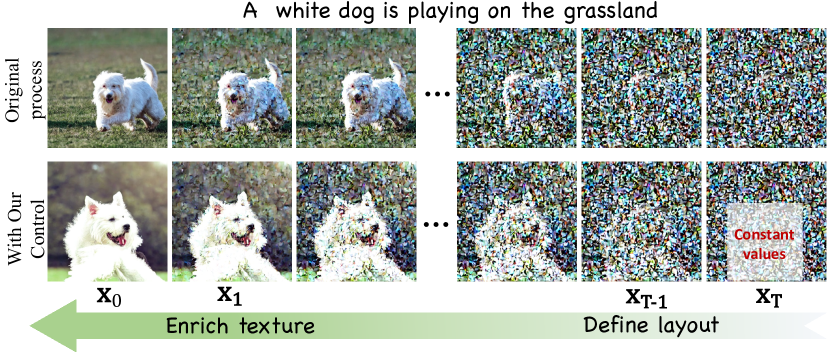
Figure 2: Top: general reverse diffusion process; Bottom: a reverse diffusion when adding small constant values to a region in the initial noise. The altered region defines the location and size of the synthesised object.

The main contributions of this paper are summarised as follows:

• We first introduce the concept of visual guidance to achieve spatial controllability in conditional diffusion models.

• We propose the Layered Rendering Diffusion to circumvent issues like unintended conceptual blending or concept mismatches that happen during the generation of multiple concepts.

• Three applications are enabled by the proposed method: bounding box-to-image, instance mask-to-image, and image editing.

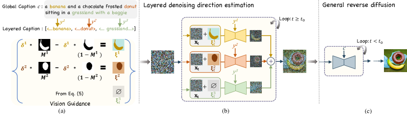
Figure 3: Overview of our approach. (a) For synthesising a sense, the user provides the global caption, layered caption as well as the spatial layout entities which are used to construct the vision guidance. LRDiff divides the reverse-time diffusion process into two sections: (b) When $t\geq t_{0}$, each vision guidance is employed into separate layers to alter the denoising direction, ensuring each object contour generates within specific regions. (c) When $t<t_{0}$, we perform the general reverse diffusion process to generate texture details that are consistent with the global caption.

2 Related Works

Text-to-Image (T2I) Models. To adhere to some specifications described by free-form text in image generation, T2I typically models the image distribution along with the encoded latent embeddings of the text prompts as the condition entities via pre-trained language models, such as CLIP [42]. Large-scale text-to-image models can be categorised as auto-regressive models [44, 11, 13, 59] and diffusion-based models [37, 45, 43, 47]. Inspired by non-equilibrium statistical physics, Dickstein et al. [48] pioneeringly introduced the diffusion model, the concept of which is revisited in Sec. 3. To accelerate training and sampling speed, the latent diffusion model [45], a.k.a. Stable Diffusion (SD) is developed to operate the diffusion process in the latent space [12] instead of the pixel space. However, when it comes to the intricate spatial semantic arrangement of multiple objects within a scene, T2I diffusion models fall short, exhibiting object leakage and a lack of awareness regarding spatial dependencies.

Layout-to-Image (L2I) Diffusion Models. Current layout-guided generation methods can be broadly classified into two main categories based on the necessity of a training process: (1) methods that involve fine-tuning diffusion models [30, 57, 61, 7, 8, 35, 55, 40, 63, 27, 24], and (2) training-free approaches [9, 41, 54, 16, 4, 28, 60, 39, 62, 32, 64, 58, 3, 29]. The former achieves locality-awareness by incorporating layout information as an additional condition to the pre-trained T2I diffusion model. Methods necessitating fine-tuning, like ControlNet[61], GLIGEN [30] and T2I-Adaptor [35] integrate extra modules into the backbone network. These modules work in concert with spatial control entities to ensure the generated images match the specified spatial conditions. ReCo [57] and GeoDiffusion [7] augment the textual tokens by incorporating new positional tokens arranged in sequences akin to short natural language sentences. However, it’s worth noting that these approaches require further training on curated datasets collected with paired annotations, which imposes significant computational and labour costs, bottlenecking applications in an open world. On the other hand, the second group of methods, such as Paint-with-words (eDiffi-Pww) [2] and ZestGuide [9], endows T2I diffusion models with localisation abilities through manipulating the cross-attention maps in the estimator network, amplifying the attention score for the text tokens that specify an object. However, when the initial noise does not tend to generate the target objects, it is difficult to change the direction of denoising by only manipulating the attention map. Besides, these methods are likely to cause the blending of appearances of adjacent objects sharing the same visual concept. This issue is exemplified in the first and second columns of Fig. 5, where the phenomenon is clearly observable.

Image Editing with Diffusion Models. Image editing, as a fundamental task in computer graphics, can be achieved by modifying a real image by inputting auxiliary entities, including scribble [33], mask [1], or reference image [6]. Recent models for text-conditioned image editing [18, 25, 33, 10] harness CLIP [42] embedding guidance combined with pre-trained T2I diffusion models, achieving excellent results across a range of editing tasks. Research in this field primarily advances along three directions: (1) zero-shot algorithms that steer the denoising process towards a desired CLIP embedding direction by manipulating the attention maps of the cross-attention mechanisms [17, 38, 33, 34, 26]; (2) textual token vector optimisation  [46, 14]; (3) fine-tuning T2I diffusion models on curated datasets with matched annotations [6, 36]. In contrast to prior works that rely on text prompts to guide the editing, we aim to leverage the proposed vision guidance information to better assist the generation process.

3 Preliminaries

Denoising Diffusion Probabilistic Models (DDPMs). DDPM [20] involves a forward-time diffusion process and a reverse-time denoising process from a prior distribution. Let $\mathbf{x}_{0}\in\mathbb{R}^{h\times w\times D}$ be a sample from the data distribution $p_{0}(\mathbf{x})$. When using a total of $T$ noise scales in the forward-time diffusion process, the discrete Markov chain is

$$\mathbf{x}_{t}=\sqrt{1-\beta_{t}}\mathbf{x}_{t-1}+\sqrt{\beta_{t}}{\epsilon}_{t-1},\quad t=1,\cdots,T~{}~{}~{}~{},$$ (1)

where ${\epsilon}_{t}$ denotes the noise sampled from $\mathcal{N}\big{(}\mathbf{0},\mathbf{I}\big{)}$ at timestep $t$, $\{\beta_{t}\}_{t=1}^{T}$ is a pre-defined variance schedule. When recursively applying the noise perturbations Eq. 1 to a real sample $\mathbf{x}_{0}\sim p_{0}(\mathbf{x})$, it ends up with $\mathbf{x}_{T}\sim\mathcal{N}\big{(}\mathbf{0},\mathbf{I}\big{)}$.

The reverse-time denoising process can be defined as:

$$\mathbf{x}_{t-1} =\tilde{\alpha}_{t}\mathbf{x}_{t}+\underbrace{\tilde{\beta}_{t}\nabla_{\mathbf{x}}\log p_{t}(\mathbf{x})}_{\text{direction pointing to }\mathbf{x}_{t}}+\underbrace{\sigma_{t}{\epsilon}_{t}}_{\text{random noise}},$$ (2)

$$\approx\tilde{\alpha}_{t}\mathbf{x}_{t}+\underbrace{\tilde{\beta}_{t}\hat{\mathbf{s}}_{t}}_{\text{estimated direction pointing to }\mathbf{x}_{t}}+\underbrace{\sigma_{t}{\epsilon}_{t}}_{\text{random noise}}.$$

where $\tilde{\alpha}_{t}$, $\tilde{\beta}_{t}$, and $\sigma_{t}$ denote the coefficients, the values of which can be derived from $\beta$. Practically, the score of the perturbed data distribution, $\nabla_{\mathbf{x}}\log p_{t}(\mathbf{x})$ for all $t$, can be estimated with a score network $\mathbf{s}_{\bm{\theta}}(\mathbf{x}_{t},t)$ optimised by using score matching [23, 50]. After training to get the optimal solution $\hat{\mathbf{s}}_{t}=\mathbf{s}_{\bm{\theta}}^{*}(\mathbf{x}_{t},t)\approx\nabla_{\mathbf{x}}\log p_{t}(\mathbf{x})$, new samples can be generated by starting from $\mathbf{x}_{T}\sim\mathcal{N}\big{(}\mathbf{0},\mathbf{I}\big{)}$ by recursively applying the estimated reverse-time process.

Following classifier-free guidance [21], the implicit update direction $\hat{\mathbf{s}}_{t}$ can be considered in the following form

$$\hat{\mathbf{s}}_{t} =\gamma\mathbf{s}_{\bm{\theta}}(\mathbf{x}_{t},t,c)+(1-\gamma)\mathbf{s}_{\bm{\theta}}(\mathbf{x}_{t},t,\varnothing),$$ (3)

where $\mathbf{s}_{\bm{\theta}}(\mathbf{x}_{t},t,\varnothing)$ is referred to as as an unconditional model, $\gamma\geq 1$ controls the guidance strength of a condition $c\in\mathcal{C}$. Trivially increasing $\gamma$ will amplify the effect of conditional input. Condition space $\mathcal{C}$ can be further defined to be text words, called text prompt [37], fundamentalising current T2I models.

4 Method

Given a global text caption and the specified layout of the scene, our method can generate images with accurate alignments, as demonstrated on the left side from Fig 1. The remainder of this section is organised as follows: We first introduce the concept of vision guidance, whose role is to leave clues for the score estimate network to steer the denoising direction of a single visual concept within a specified region. Subsequently, we develop the Layered Rendering Diffusion (LRDiff) framework that constructs an image-rendering process with multiple layers, incorporating vision guidance at each layer for enhanced precision.

4.1 Vision Guidance

We introduce vision guidance, denoted as $\bm{\xi}\in\mathbb{R}^{h\times w\times D}$, as an additional condition to the score estimate network, forming $\mathbf{s}_{\bm{\theta}}(\mathbf{x}_{(t)},~{}t,~{}c,~{}\bm{\xi})$. Furthermore, the vision guidance entities are input into the network in a zero-shot form:

$$\mathbf{s}_{\bm{\theta}}(\mathbf{x}_{t},~{}t,~{}c,~{}\bm{\xi})=\mathbf{s}_{\bm{\theta}}(\mathbf{x}_{t}{+}\bm{\xi},~{}t,~{}c).$$ (4)

A significant advantage of this zero-shot paradigm is that the introduction of the additional condition has no re-training requirement for off-the-shell conditional diffusion models, thereby substantially reducing computational costs.

The Definition. We factorise the vision guidance condition into two components: a vector $\bm{\delta}\in\mathbb{R}^{D}$ and a binary mask $\bm{\mathcal{M}}\in\{0,1\}^{h\times w}$. Each element $\xi_{j,k,l}$ of $\bm{\xi}$ is defined as follows:

$$\xi_{j,k,l} =\delta_{l}\cdot\mathcal{M}_{j,k}-\delta_{l}\cdot(1-\mathcal{M}_{j,k}),$$ (5)

$$=\delta_{l}\cdot(2\mathcal{M}_{j,k}-1),$$

where $\mathcal{M}_{j,k}$ is assigned the value 1 if the spatial position $({j,k})$ falls within the expected object region. For the region containing an object, we add $\bm{\delta}$ to enhance the generation tendency of that object. Conversely, for areas outside the target region, we subtract $\bm{\delta}$ to suppress the generation tendency of the object. The binary mask $\bm{\mathcal{M}}$ can be derived from user input, such as converting a bounding box or instance mask provided by the user into the binary mask. Next, we introduce two distinct approaches to compute the vector $\bm{\delta}$.

Constant vector: A nativ̈e approach for the configuration is to set the vector $\bm{\delta}$ to some constant values. When the diffusion model operates in the RGB space, we can set $\bm{\delta}$ to constant values corresponding to some colour described by the text prompt (e.g., $[0.3,0.3,0.3]$ corresponding to a white colour with transparency). When operating in the latent space of VAE, $\bm{\delta}$ can be set to the latent representation of the constant values when operations such as dimension expansion and tensor repeat are required. Although the manual adjustment $\bm{\delta}$ to some constant values is versatile to generate objects with various visual concepts, it necessitates human intervention.

Dynamic vector: Beyond simply assigning constant values to $\bm{\delta}$, we propose to dynamically adapt the values of $\bm{\delta}$ based on the input text conditions in order to reduce human intervention during generation. In this context, we consider the implementation of Stable Diffusion [45] wherein text tokens are interconnected with the visual features via cross-attention modules. At the initial denoising step, i.e., $t=T$, we extract the cross-attention map $\mathbf{A}\in\mathbb{R}^{|c|\times hw}$ from an intermediate layer in the U-Net. For a more straightforward illustration, we will consider the synthesis of an image containing a single object, corresponding to the $i$-th text token from the text prompt $c$. Subsequently, to derive the vector $\bm{\delta}$ in Eq. 5, we perform the following operations:

$$\bm{S} =\{(j,k)|\mathbf{A}_{j,k}^{i}>\mathrm{Threshold}_{K}(\mathbf{A}^{i})\},$$ (6)

$$\bm{\delta} =\frac{\lambda}{|\bm{S}|}\sum\{\mathbf{x}_{t}(j,k)|(j,k)\in\bm{S}\},$$

where $\mathbf{x}_{t}(j,k)$ denotes the element at spatial location $(j,k)$ in $\mathbf{x}_{t}$. The $\sum$ operation sums up all items within the $\bm{S}$ set. Additionally, the operation $\mathrm{Threshold}_{K}(\cdot)$ selects the $K$-th largest value from the top $K$ values in $\mathbf{A}^{i}$. The strength of vision guidance is modulated by the coefficient $\lambda$, alongside the classifier-free guidance coefficient $\gamma$. Given the presence of multiple cross-attention blocks within the score network, we opt to select the block following the down-sampling in each stage and subsequently average their outputs.

4.2 Layered Rendering

Considering an upcoming image drawing $n$ objects, we encapsulate all the condition entries of the diffusion model into the following

$$\mathrm{Global~{}Caption:} ~{}~{}~{}~{}c,$$ (7)

$$\mathrm{Layered~{}Captions:} ~{}~{}~{}~{}[y^{1}(c),\cdots,y^{n}(c)],$$

$$\mathrm{Vision~{}Guidance:} ~{}~{}~{}~{}[\bm{\xi}^{1},\cdots,\bm{\xi}^{n}],$$

$$\mathrm{Layered~{}Masks:} ~{}~{}~{}~{}[\bm{\mathcal{M}}^{1},\cdots,\bm{\mathcal{M}}^{n}],$$

where we define a set of mappings $y^{i}:\mathcal{C}\rightarrow\mathcal{Y}$, and $y^{i}(c)$  represents the text condition for layer $i$. $\bm{\xi}^{i}$ is the vision guidance for the $i_{th}$ object constructed by the $\bm{\mathcal{M}}^{i}$ and $\delta^{i}$. Appendix A from our supplementary material details the implementation of layered prompt construction.

As mentioned in Sec. 1, our layered rendering algorithm divides the full reverse-time denoising process into two denoising sections, i.e. $[T,\cdots,t_{0}],~{}[t_{0}{-}1,\cdots,1]$. At each timestep $t\in[T,\cdots,t_{0}]$,

the denoising process is given by

$$\mathbf{x}_{t{-}1} =\tilde{\alpha}_{t}\mathbf{x}_{t}+\tilde{\beta}_{t}[\gamma~{}\bm{\Phi}_{t}+(1-\gamma)\mathbf{s}_{\bm{\theta}}(\mathbf{x}_{t},t,\varnothing)]+\sigma_{t}{\epsilon}_{t},$$ (8a)

$$\bm{\Phi}_{t} =\sum_{i=1}^{n}\frac{\bm{\mathcal{M}}^{i}}{\sum_{i=1}^{n}\bm{\mathcal{M}}^{i}}\otimes\mathbf{s}_{\bm{\theta}}(\mathbf{x}_{t}{+}\bm{\xi}^{i},t,y^{i}).$$ (8b)

As shown in Fig. 3, we construct $\bm{\Phi}_{t}$ by fusing estimated noises in each layer and sending it into the next denoising loop. Eq. 8 assures that the prediction $\mathbf{x}_{t{-}1}$ for any step from $[T,\cdots,t_{0}]$ is within the data distribution $p_{t}(\mathbf{x})$, so that the score network $\mathbf{s}_{\bm{\theta}}$ needs no fine-tuning. The derivation process of Eq. 8 is provided in Appendix B. We carry out the layered generative process along with vision guidance as expressed in Eq. 8 for $[T,\cdots,t_{0}]$. For timesteps in the second denoising section, e.g., $[t_{0}{-}1,\cdots,1]$, we perform the standard denoising process but with the global caption $c$ as the solid condition information, illustrated in the third column in Fig 3. The overall generative process is described by Algorithm 1.

Algorithm 1 Layered Rendering Diffusion

1:Input: $c,~{}[y^{1},\cdots,y^{n}],~{}[\bm{\mathcal{M}}^{1},\cdots,\bm{\mathcal{M}}^{n}]$,

2: Pre-trained diffusion model $\mathbf{s}_{{\bm{\theta}}}$;

3: Initialise $\mathbf{x}_{T}$ $\triangleright$ Noise initialisation

4: $[\bm{\xi}^{1},...,\bm{\xi}^{n}]$ $\leftarrow$ Calculate Eq. 6

5:for $t=T,\cdots,t_{0}$ do

6:      $\triangleright$ Estimate layered denoising direction

7:      $\bm{\Phi}_{t}$ $\leftarrow$ Calculate Eq. 8b

8:      $\mathbf{x}_{t{-}1}$ $\leftarrow$ Calculate Eq. 8a

9:      $\mathbf{x}_{t}=\mathbf{x}_{t-1}$

10:for $t=t_{0}{-}1,\cdots,1$ do

11:      $\triangleright$ Estimate general denoising direction

12:      $\hat{\mathbf{s}}_{t}=\mathbf{s}_{\bm{\theta}}(\mathbf{x}_{t},t)+\gamma\big{(}\mathbf{s}_{\bm{\theta}}(\mathbf{x}_{t},t,\mathcal{C})-\mathbf{s}_{\bm{\theta}}(\mathbf{x}_{t},t)\big{)}$

13:      $\mathbf{x}_{t-1}=\tilde{\alpha}_{t}\mathbf{x}_{t}+\tilde{\beta}_{t}\hat{\mathbf{s}}_{t}+\sigma_{t}{\epsilon}_{t}$

14:      $\mathbf{x}_{t}=\mathbf{x}_{t-1}$

15:Output: $\mathbf{x}_{0}$

The framework of our method is illustrated in Fig. 3. We assign a null value $\varnothing$ to the vision guidance $\bm{\xi}^{n}$ in the final layer(e.g., the $3^{\mathrm{rd}}$ layer in Fig. 3), encompassing scene descriptions or other objects without defined layouts.

5 Image Editing with Layout

In addition to instance mask-to-image and bounding box-to-image tasks, our approach extends to image editing, leveraging layered rendering techniques. We employ the DDIM inversion technique [49] to obtain the noise latent representation. This inverted latent noise serves as the final layer (e.g., the $3^{\mathrm{rd}}$ layer in Fig. 3) in our pipeline, enabling further processing. As demonstrated in Fig.4 and the right side of Fig1, our method allows inserting objects of various sizes at different locations within a provided image. For instance, we can add hats of different sizes to the dogs. Also, we can replace objects in specific areas of the provided image, such as substituting a teapot with a bottle. Thanks to our layered rendering technology, the edited images seamlessly fit the given prompts, while keeping other areas of content as unchanged as possible.

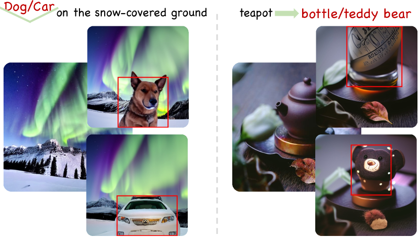
Figure 4: Example results of image editing. Left: adding objects into images; Right: replacing the object at the specified position.

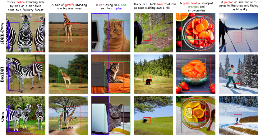
Figure 5: Quantitative comparisons of methods that use bounding box entities as the spatial condition. Our results show better spatial alignments than other methods.

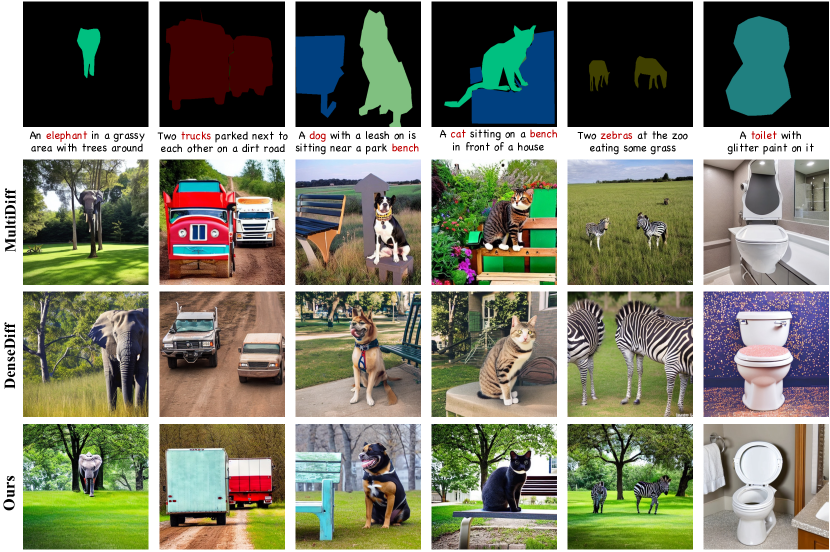
Figure 6: Quantitative comparisons of methods that use instance mask entities as the spatial condition. Our results show better spatial alignments than other methods.

6 Experiments

Dataset and Implementation Details. All the experiments are run in a single NVIDIA Tesla V100. Unless specified otherwise, we use the DDIM sampler [49] with 50 sampling steps for the reverse diffusion process with a fixed guidance scale of 7.5; $t_{0}$ is set to 15 by default. We construct our dataset by selecting 1134 captions with one or more objects and corresponding bounding boxes or instance masks from the MS-COCO validation set [31]. Details can be found in Appendix A.

Bounding Box	Image-Score		Align-Score
	T2I-Sim$\uparrow$	CLIP$\uparrow$	AP$\uparrow$	$\mathrm{AP}_{50}$$\uparrow$	$\mathrm{AP}_{75}$$\uparrow$
SD [45]	0.292	0.316	-	-	-
TwFA [56]	0.210	0.179	9.9	16.3	9.0
eDiffi-Pww [2]	0.279	0.299	4.2	8.6	4.0
BoxDiff [54]	0.295	0.319	5.8	17.2	3.0
LRDiff(Ours)	0.281	0.292	17.4	35.6	15.5

Table 1: The quantitative results of bounding box input.

Instance Mask	Image-Score		Align-Score
	T2I-Sim$\uparrow$	CLIP$\uparrow$	$\mathrm{AP}_{50}$$\uparrow$	$\mathrm{AP}_{75}$$\uparrow$	IOU$\uparrow$
SD [45]	0.292	0.316	-	-	-
eDiffi-Pww [2]	0.287	0.304	16.5	6.4	33.11
MultiDiff [4]	0.277	0.281	30.9	8.2	47.59
DenseDiff. [28]	0.289	0.310	11.3	1.3	27.65
LRDiff(Ours)	0.280	0.295	35.0	15.4	49.06

Table 2: The quantitative results of instance mask input.

Evaluation Metrics. For evaluating synthesised images with both bounding box and instance mask inputs, we employ two distinct metrics: image-score and align-score. The image-score specifically measures the fidelity of the synthesised image to the text prompt, incorporating sub-indicators such as T2I-Sim [54] and the CLIP score [19] for a nuanced assessment. On the other hand, the align-score evaluates the image’s spatial alignment with the given layout condition, using the AP results predicted by YOLOv4 as a benchmark for alignment accuracy. Additionally, regarding instance mask inputs, we assess the precision of object contours using the IoU scores produced by employing YOLOv7 [51] and the ground truth.

6.1 Bounding boxes as layout condition

Quantitative comparison. In Table 1, we present a comparative analysis of our method against BoxDiff [54], eDiffi-Pww [2], and TwFA [56]. Our evaluation revealed a trade-off relationship between the align-score and image-score among the compared methods. For instance, while TwFA [56] achieved superior alignment scores compared to other diffusion methods, its limited image generation capabilities led to lower-quality generated backgrounds. Consequently, this facilitated easier foreground differentiation by YOLO [5], resulting in higher detection metrics. To ensure fairness in comparisons, we established SD [45] as the baseline for the image-score. Notably, our results exhibited higher AP values in contrast to eDiffi-Pww and TwFA, while closely aligning with the baseline in terms of image-score. Furthermore, our image-score values are close to those of BoxDiff, but our three alignment score sub-metrics exceed BoxDiff by 11.6%, 17.6%, and 12.5%, respectively.

Qualitative comparison. Fig. 5 presents qualitative comparisons among various methods in a multi-object layout. According to the results, LRDiff can effectively mitigate the issue of visual blending between adjacent objects within the same category, which is a challenge for other methods such as BoxDiff [54] and eDiffi-Pww [2]. This effectiveness is exemplified in the synthesis of giraffes, as shown in the second column of Fig. 5. Furthermore, our method surpasses eDiffi-Pww when synthesising images within intricate layouts. Notably, in the third column, where a cat, bed and laptop are closely arranged, our LRDiff proficiently handles mutual occlusion, underscoring its capability to manage complex scene compositions. Additionally, our approach shows high fidelity in generating small-scale objects, which remains challenging for the listed methods that rely on manipulating cross-attention maps to control layout.

6.2 Instance masks as layout condition

Quantitative comparison. The instance masks, serving as layout guides, provide both positional and contour details. As highlighted in Table 2, our approach outperforms other diffusion-based zero-shot techniques [28, 4, 2] in the IoU metric. Similar to the analysis in subsection. 6.1, there is a trade-off correlation between the image-score and align-score. Our results significantly outperform eDiffi-Pww and DenseDiff by over 16% and 22%, respectively, in the IOU metric while closely aligning with their image-score outcomes. The observed low image-score in MultiDiff [4] is attributed to its limited interaction with global captions, leading to a ‘copy-paste-like’ phenomenon. In contrast, our method integrates all layers and interacts with global captions after delineating object outlines in layers. Consequently, compared to MultiDiff [4], our method achieves a closer alignment with the baseline image-score, surpassing it by 1.6% in the mIoU metric. Furthermore, substantial enhancements in both $AP_{50}$ and $AP_{75}$ indicators by over 9% each signify the accurate alignment and positioning of generated objects within the specified mask area, validating the efficacy of our approach.

Qualitative comparison. Fig.6 presents qualitative comparisons between our method and others across both single and multi-object layouts. The results highlight our effectiveness in generating small-scale objects, which is still a challenge for DenseDiff [28]. Examples to justify our effectiveness are provided in the first and fifth columns of Fig.6 where the synthesised elephants and zebras are faithful to the shapes provided in the layout entity. MultiDiff [4] demonstrates high effectiveness in achieving precise spatial alignment within images. However, it exhibits limitations in harmonising the overall image composition, occasionally resulting in a ‘copy-paste’ result. This inadequacy is particularly evident in the first and last columns of the figure, where an elephant appears inserted into a tree and a toilet lacks seamless integration with the surrounding environment. Conversely, our method ensures precise image layout accuracy by employing visual guidance and achieves seamless integration throughout the entire image due to the fusion of all layers and interaction with the global captions.

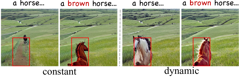
Figure 7: The difference impacts of using constant vision guidance and dynamic vision guidance.

6.3 Ablation Study

We compare the impacts of two approaches in calculating vectors for vision guidance, the influence of different $t_{0}$ values, and the robustness of our method to diverse scene descriptions. Further ablation experiments and detailed results are provided in Appendix A.

Constant vs. Dynamic. We conducted a visualisation analysis, showcased in Fig. 7, to compare the effects of two approaches in calculating vector $\bm{\delta}$ for vision guidance. Our synthesis focused on depicting scenarios such as a horse” or a brown horse” running on grassland at specific locations. For this, $\bm{\delta}$ was assigned values corresponding to the colour brown. In scenarios where the text prompt omits a brown colour description, the model sometimes erroneously generates a road of a similar colour, resulting in a mismatch with the text description. However, when the text prompt explicitly includes a colour description, the resulting synthesised image exhibits high faithfulness to the text description. On the other hand, the dynamic vector strategy always shows high spatial alignment to the given layout, regardless of the existence of colour description in the text prompt.

The impact of different $t_{0}$. LRDiff divides the reverse diffusion process into two denoising sections: $[T,\cdots,t_{0}],~{}[t_{0}{-}1,\cdots,1]$. As we analyse in Fig. 8, a longer first denoising period (i.e., $|T-t_{0}|$) will generate images of higher spatial aliment with the given spatial layout. However, a short first denoising period can result in less precise spatial alignment. We attribute this raised deviation to the ambiguity in object shapes during the early denoising steps, where they are particularly susceptible to noise from other layers. We observe that setting $|T-t_{0}|=15$ usually gives some decent results. The lower part in Fig. 8 shows that when setting $|T-t_{0}|=15$ the knife’s shape fits better than the others.

Robustness to Diverse Scene Descriptions: As depicted in Fig. 9, we examined the performance of our method with various scene descriptions, placing the tiger or giraffe in different settings such as ‘a desert with a blue sky’ or ‘a garden with flowers.’ The results demonstrate that alterations in the scene description do not impact the positional and shape consistency of the target object relative to the specified layout.

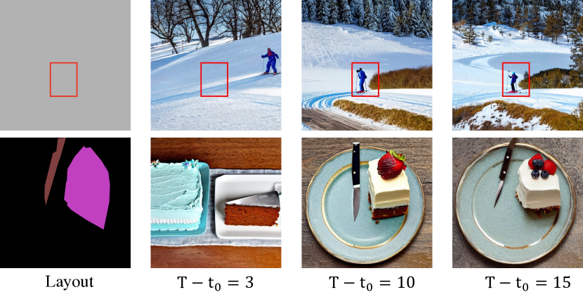
Figure 8: The impacts of different $t_{0}$.

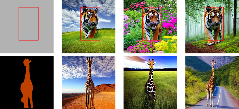
Figure 9: The results of various scene descriptions.

7 Conclusion

In this paper, we start with an observation that suggests that changing the mean value of a local area in the initial noise can steer the direction of the denoising process. Based on this insight, our work introduces the notion of vision guidance, serving as a cue for the network to adjust the denoising direction in single object generation. Subsequently, we propose the Layered Rendering Diffusion (LRDiff) framework that constructs an image-rendering process with multiple layers, each of which employs vision guidance to ensure precise spatial alignment of individual objects. Our technology is applied across three applications: bounding box-to-image, instance mask-to-image, and image editing. Finally, the experiments demonstrate the effectiveness of our method.

Appendix A The Derivation of Layered Rendering

In order to ensure that the prediction $\tilde{\mathbf{x}}_{t{-}1}$ for any step from $[T,\cdots,t_{0}]$ is within the data distribution $p_{t}(\mathbf{x})$ with the pre-trained score network $\mathbf{s}_{\bm{\theta}}$, the Layered Rendering method (i.e., Eq.(8) from the main paper) is proposed by solving the following objective

$$\arg\min_{\tilde{\mathbf{x}}_{t}\in\mathcal{I}_{t}}\sum_{i=1}^{n}\left\|\bm{\mathcal{M}}_{i}\otimes\left(\tilde{\mathbf{x}}_{t{-}1}-\mathbf{x}_{t{-}1}^{i}\right)\right\|^{2},$$ (9)

where $\{\mathbf{x}_{t{-}1}^{i}\}_{i=1}^{n}$ is referred to as the results of $n$ independent denoising processes at timestep $t$; $\tilde{\mathbf{x}}_{t{-}1}$ is referred to as the desired result that integrates information from $\{\mathbf{x}_{t{-}1}^{i}\}_{i=1}^{n}$ based on the provided region contains from $\{\bm{\mathcal{M}}_{i}\}_{i=1}^{n}$.

The analytical solution to this objective is given by

$$\sum_{i=1}^{n}\bm{\mathcal{M}}_{i}\otimes\tilde{\mathbf{x}}_{t{-}1} =\sum_{i=1}^{n}\bm{\mathcal{M}}_{i}\otimes\mathbf{x}_{t{-}1}^{i}$$ (10)

$$\therefore\tilde{\mathbf{x}}_{t{-}1}=\frac{1}{\sum_{i=1}^{n}\bm{\mathcal{M}}_{i}}\sum_{i=1}^{n}\bm{\mathcal{M}}_{i}\otimes\mathbf{x}_{t{-}1}^{i}=\sum_{i=1}^{n}\frac{\bm{\mathcal{M}}^{i}}{\sum_{i=1}^{n}\bm{\mathcal{M}}^{i}}\otimes\mathbf{x}_{t{-}1}^{i}.$$ (11)

According to the reverse-time diffusion definition,

$$\mathbf{x}_{t{-}1}^{i}\approx\tilde{\alpha}_{t}\mathbf{x}_{t}+\underbrace{\tilde{\beta}_{t}\hat{\mathbf{s}}_{t}^{i}}_{\text{estimated direction pointing to }\mathbf{x}_{t}^{i}}+\underbrace{\sigma_{t}{\epsilon}_{t}^{i}}_{\text{random noise}},$$ (12)

we have

$$\tilde{\mathbf{x}}_{t{-}1} =\sum_{i=1}^{n}\frac{\bm{\mathcal{M}}^{i}}{\sum_{i=1}^{n}\bm{\mathcal{M}}^{i}}\otimes\left(\tilde{\alpha_{t}}\mathbf{x}_{t}^{i}+\tilde{\beta_{t}}\hat{\mathbf{s}}_{t}^{i}+\sigma_{t}\epsilon_{t}^{i}\right)$$ (13)

$$=\tilde{\alpha_{t}}\left(\sum_{i=1}^{n}\frac{\bm{\mathcal{M}}^{i}}{\sum_{i=1}^{n}\bm{\mathcal{M}}^{i}}\otimes\mathbf{x}_{t}^{i}\right)+\tilde{\beta_{t}}\left(\sum_{i=1}^{n}\frac{\bm{\mathcal{M}}^{i}}{\sum_{i=1}^{n}\bm{\mathcal{M}}^{i}}\otimes\hat{\mathbf{s}}_{t}^{i}\right)+\sigma_{t}\left(\sum_{i=1}^{n}\frac{\bm{\mathcal{M}}^{i}}{\sum_{i=1}^{n}\bm{\mathcal{M}}^{i}}\otimes{\epsilon}_{t}^{i}\right)$$

$$=\tilde{\alpha_{t}}\tilde{\mathbf{x}}_{t}+\tilde{\beta_{t}}\left(\sum_{i=1}^{n}\frac{\bm{\mathcal{M}}^{i}}{\sum_{i=1}^{n}\bm{\mathcal{M}}^{i}}\otimes\hat{\mathbf{s}}_{t}^{i}\right)+\sigma_{t}\tilde{\epsilon}_{t}\quad\quad(\mathrm{Apply}~{}\lx@cref{creftype~refnum}{eqn: anal})$$

$$=\tilde{\alpha}_{t}\tilde{\mathbf{x}}_{t}+\tilde{\beta}_{t}\left\{\sum_{i=1}^{n}\frac{\bm{\mathcal{M}}^{i}}{\sum_{i=1}^{n}\bm{\mathcal{M}}^{i}}\otimes\left[\gamma~{}\mathbf{s}_{\bm{\theta}}(\tilde{\mathbf{x}}_{t}{+}\bm{\xi}^{i},t,y^{i})+(1-\gamma)\mathbf{s}_{\bm{\theta}}(\tilde{\mathbf{x}}_{t},t,\varnothing)\right]\right\}+\sigma_{t}\tilde{{\epsilon}}_{t}\quad\quad\quad(\mathrm{Apply~{}CFG})$$

$$=\tilde{\alpha}_{t}\tilde{\mathbf{x}}_{t}+\tilde{\beta}_{t}\left\{\gamma\left[\sum_{i=1}^{n}\frac{\bm{\mathcal{M}}^{i}}{\sum_{i=1}^{n}\bm{\mathcal{M}}^{i}}\otimes\mathbf{s}_{\bm{\theta}}(\tilde{\mathbf{x}}_{t}{+}\bm{\xi}^{i},t,y^{i})\right]+(1-\gamma)\mathbf{s}_{\bm{\theta}}(\tilde{\mathbf{x}}_{t},t,\varnothing)\right\}+\sigma_{t}\tilde{{\epsilon}}_{t}$$

Let $\bm{\Phi}_{t}$ be the compositional estimation at timestep $t$:

$$\bm{\Phi}_{t}=\sum_{i=1}^{n}\frac{\bm{\mathcal{M}}^{i}}{\sum_{i=1}^{n}\bm{\mathcal{M}}^{i}}\otimes\mathbf{s}_{\bm{\theta}}(\tilde{\mathbf{x}}_{t}{+}\bm{\xi}^{i},t,y^{i}).$$ (14)

Finally, we have

$$\tilde{\mathbf{x}}_{t{-}1}=\tilde{\alpha}_{t}\tilde{\mathbf{x}}_{t}+\tilde{\beta}_{t}\left[\gamma~{}\bm{\Phi}_{t}+(1-\gamma)\mathbf{s}_{\bm{\theta}}(\tilde{\mathbf{x}}_{t},t,\varnothing)\right]+\sigma_{t}\tilde{{\epsilon}}_{t}.$$ (15)

Appendix B Dataset Construction

We construct a dataset comprising 1,134 global captions along with corresponding bounding boxes, object categories, and instance masks sourced from the MS COCO dataset. The dataset encompasses 55 categories in total (including 11 animal classes and 44 object classes) for spatially conditional text-to-image synthesis, which is summarised in Fig. 10.

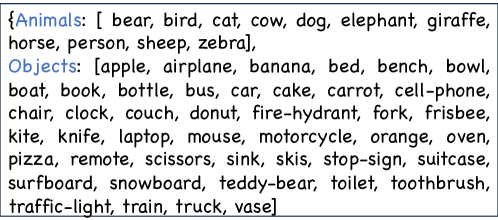
Figure 10: The constructed dataset contains 55 categories in total.

In this dataset, for the layers from $[1,n-1]$, we configured the layered captions in the form of “a $<\mathrm{category~{}name}>$”, whereas, for the final layer $n$, the scene descriptions or other object categories are extracted using LLM from the global captions. Thanks to the exceptional capability of LLM in few-shot learning, we only provide a few examples, e.g., “A bear is running the grassland”, the description of the scene is “The beautiful grassland”, and the LLM effectively extracted the context and produced a suitable response. Notably, LLM is simply used for batch processing the global captions in the dataset. In practical applications, our method supports user-defined scene descriptions or provides a default description if not specified.

Appendix C More ablation studies.

Vision Guidance with $K$ dynamic vectors. We provide an alternative implementation of vision guidance $\bm{\xi}$ with $K$ dynamic vectors. Specifically, for each position in the object area in $\bm{\xi}$, where $\mathcal{M}_{j,k}=1$, we fill the position with a vector randomly sampled from the $\mathbf{S}$ set (in Eq.(6) from the main paper). We refer to this alternative implementation as ‘multi-vectors’, contrasting it with the ‘mean-vector’ method, mentioned in Sec. 4.1 from the main paper.

Bounding Box	Image-Score		Align-Score
	T2I-Sim$\uparrow$	CLIP$\uparrow$	$\mathrm{mAP}$$\uparrow$	$\mathrm{AP}_{50}$$\uparrow$	$\mathrm{AP}_{75}$$\uparrow$
$\text{multi-vectors}_{10}$	0.278	0.293	17.0	30.0	13.9
$\text{mean-vector}_{10}$	0.284	0.298	17.2	33.2	14.6
$\text{multi-vectors}_{20}$	0.272	0.287	17.1	32.9	14.5
$\pagecolor{gray!20}{\text{mean-vector}_{20}}$	0.281	0.295	17.4	35.6	15.5

Table 3: Comparison of ‘multi-vectors’ and ‘mean-vector’ with bounding box entities. The grey line indicates the results in Table 1 from the main paper. The subscript denotes the choice of value $K$.

Instance Mask	Image-Score		Align-Score
	T2I-Sim$\uparrow$	CLIP$\uparrow$	$\mathrm{AP}_{50}$$\uparrow$	$\mathrm{AP}_{75}$$\uparrow$	IOU$\uparrow$
$\text{multi-vectors}_{10}$	0.281	0.296	36.5	19.2	49.02
$\text{mean-vector}_{10}$	0.277	0.287	37.9	19.8	49.41
$\text{multi-vector}_{20}$	0.278	0.292	40.5	21.0	49.54
$\pagecolor{gray!20}{\text{mean-vector}_{20}}$	0.280	0.295	35.0	15.4	49.06

Table 4: Comparison of ‘multi-vectors’ and ‘mean-vector’ with instance mask entities. The grey line shows the results in Table 2 from the main paper. The subscript denotes the choice of value $K$.

In Table 4 and Table 4, we illustrate the varying impacts of employing different construction methods under both instance mask and bounding box conditions. The tables highlight the remarkable similarity in results obtained through these two different approaches to constructing dynamic vectors. Notably, while the outcomes align closely, the ‘mean-vector’ method better aligns with the input text compared to the ‘multi-vectors’. Observing the influence of different $K$ values, it’s evident that when $K$ is set to 10, the image-score outperforms that achieved when $K$ is set to 20. However, the align-score exhibits higher values when $K$ is set to 20. To ensure a balanced performance between image-score and align-score, we opt for the ‘mean-vector’ method with $K$ set to 20.

While ‘mean-vector’ outperforms ‘multi-vectors’ in both image-score and align-score metrics, the latter demonstrates advantages in texture diversity in specific instances. Illustrated in Fig. 11, an example clarifies the divergent visual effects of employing these two approaches. Notably, the ‘mean-vector’ method yields donuts with similar colours, whereas the ‘multi-vectors’ method generates donuts exhibiting a spectrum of colours. This discrepancy arises due to the ‘mean-vector’ constructing the dynamic vector based on a single outcome (the mean of $\{\mathbf{x}_{t}(j,k),(j,k)\in\mathbf{S}\}$), while ‘multi-vectors’ generates $K$ outcomes (various $\mathbf{x}_{t}(j,k)$) randomly added to the target area, introducing randomness and resulting in varied colours. This diversity proves advantageous, especially when multiple objects of the same category appear in a scene. However, in most cases, the ‘mean-vector’ method suffices entirely.

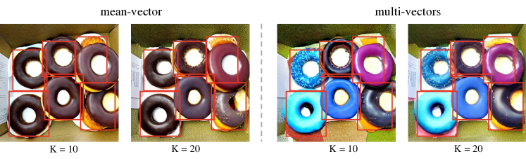
Figure 11: The varying impacts of employing different construction methods. The results of ‘multi-vectors’ demonstrate advantages in texture diversity in specific instances.

The necessity of vision guidance. We provide an ablation to assess the necessity of vision guidance. Particularly, we experiment with the model with no vision guidance within the target areas by modifying Eq.(5) in the main paper to:

$$\xi_{j,k,l} =-\delta_{l}\cdot(1-\mathcal{M}_{j,k})$$ (16)

This modification aims to analyse the effect of not applying vision guidance in the target region. We term this as setting  #1. The combined approach of suppressing the non-target areas and enhancing the target areas, as mentioned in Sec. 4.1 from the main paper, is termed setting  #2.

Bounding Box	Image-Score		Align-Score
	T2I-Sim$\uparrow$	CLIP$\uparrow$	$\mathrm{mAP}$$\uparrow$	$\mathrm{AP}_{50}$$\uparrow$	$\mathrm{AP}_{75}$$\uparrow$
setting #1	0.1967	0.1642	1.3	3.8	0.7
setting #2	0.281	0.295	17.4	35.6	15.5

Table 5: These results depict the outcome when vision guidance is not applied within the target areas under the bounding box condition. The grey line represents the result mentioned in Table 1 from the main paper.

Instance Mask	Image-Score		Align-Score
	T2I-Sim$\uparrow$	CLIP$\uparrow$	$\mathrm{AP}_{50}$$\uparrow$	$\mathrm{AP}_{75}$$\uparrow$	IOU$\uparrow$
setting #1	0.2599	0.2767	5.2	0.8	28.16
setting #2	0.280	0.295	35.0	15.4	49.06

Table 6: These results depict the outcome when vision guidance is not applied within the target areas under the instance mask condition. The grey line represents the result mentioned in Table 2 from the main paper.

Tables 6 and 6 present a direct comparison between the results obtained with and without vision guidance in the target area. The outcomes strongly indicate that the absence of such guidance renders the results nearly unusable. Additionally, as shown in Fig. 12, the lack of vision guidance clues in the target areas makes it notably challenging for the original noise to generate specified objects.

Table. 6 illustrates that the results based on the mask may exhibit better performance compared to those based on the bounding box. While a mask provides the object’s shape, it’s notable that generating simpler shapes, such as a round pizza, might be feasible without vision guidance but tends to lack realism. Conversely, more intricate shapes, like zebras, are more likely to fail. Considering the findings from these tables and figures, it can be concluded that vision guidance significantly impacts the effectiveness of the generated outcomes.

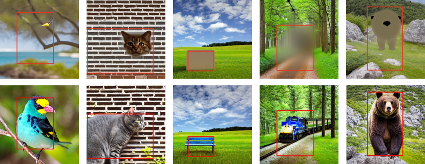
Figure 12: The first row (setting #1) shows example results that apply vision guidance in the target areas, whilst the second row (setting #2) shows example results that do not employ vision guidance in the target areas.

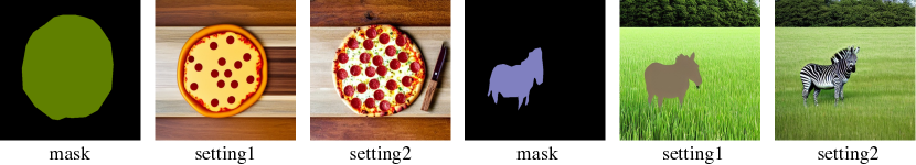
Figure 13: Setting #1: without vision guidance in the target areas. Setting #2: with vision guidance in the target areas.

Appendix D More Visualisation Results

In Fig.14, we display the intermediate results for each layer. Meanwhile, Fig.15 shows additional visualisation results obtained with different random seeds.

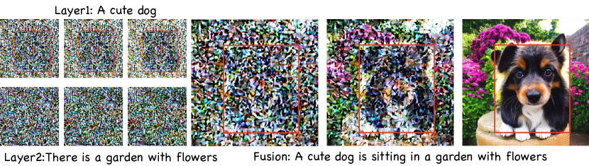
Figure 14: The visualisation of intermediate results of each layer.

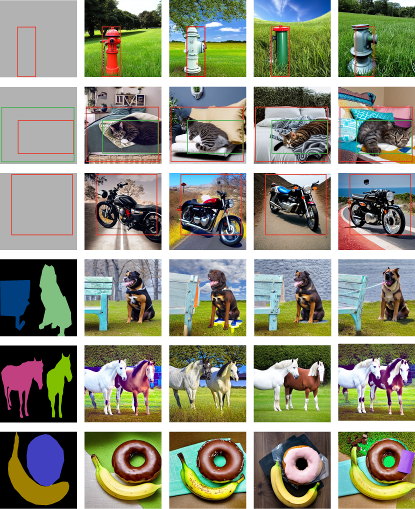
Figure 15: More visualisation results are presented using our method. Columns 2-5 showcase the outcomes with various random seeds.

References

- [1] O. Avrahami, D. Lischinski, and O. Fried. Blended diffusion for text-driven editing of natural images. In Proceedings of the IEEE/CVF Conference on Computer Vision and Pattern Recognition, pages 18208–18218, 2022.
- [2] Y. Balaji, S. Nah, X. Huang, A. Vahdat, J. Song, K. Kreis, M. Aittala, T. Aila, S. Laine, B. Catanzaro, et al. ediffi: Text-to-image diffusion models with an ensemble of expert denoisers. arXiv preprint arXiv:2211.01324, 2022.
- [3] A. Bansal, H.-M. Chu, A. Schwarzschild, S. Sengupta, M. Goldblum, J. Geiping, and T. Goldstein. Universal guidance for diffusion models. In Proceedings of the IEEE/CVF Conference on Computer Vision and Pattern Recognition, pages 843–852, 2023.
- [4] O. Bar-Tal, L. Yariv, Y. Lipman, and T. Dekel. Multidiffusion: Fusing diffusion paths for controlled image generation. arXiv preprint arXiv:2302.08113, 2023.
- [5] A. Bochkovskiy, C.-Y. Wang, and H.-Y. M. Liao. Yolov4: Optimal speed and accuracy of object detection. arXiv preprint arXiv:2004.10934, 2020.
- [6] T. Brooks, A. Holynski, and A. A. Efros. Instructpix2pix: Learning to follow image editing instructions. In Proceedings of the IEEE/CVF Conference on Computer Vision and Pattern Recognition, pages 18392–18402, 2023.
- [7] K. Chen, E. Xie, Z. Chen, L. Hong, Z. Li, and D.-Y. Yeung. Integrating geometric control into text-to-image diffusion models for high-quality detection data generation via text prompt. arXiv preprint arXiv:2306.04607, 2023.
- [8] J. Cheng, X. Liang, X. Shi, T. He, T. Xiao, and M. Li. Layoutdiffuse: Adapting foundational diffusion models for layout-to-image generation. arXiv preprint arXiv:2302.08908, 2023.
- [9] G. Couairon, M. Careil, M. Cord, S. Lathuilière, and J. Verbeek. Zero-shot spatial layout conditioning for text-to-image diffusion models. In Proceedings of the IEEE/CVF International Conference on Computer Vision, pages 2174–2183, 2023.
- [10] G. Couairon, J. Verbeek, H. Schwenk, and M. Cord. Diffedit: Diffusion-based semantic image editing with mask guidance. arXiv preprint arXiv:2210.11427, 2022.
- [11] M. Ding, Z. Yang, W. Hong, W. Zheng, C. Zhou, D. Yin, J. Lin, X. Zou, Z. Shao, H. Yang, et al. Cogview: Mastering text-to-image generation via transformers. Advances in Neural Information Processing Systems, 34:19822–19835, 2021.
- [12] P. Esser, R. Rombach, and B. Ommer. Taming transformers for high-resolution image synthesis. In Proceedings of the IEEE/CVF conference on computer vision and pattern recognition, pages 12873–12883, 2021.
- [13] O. Gafni, A. Polyak, O. Ashual, S. Sheynin, D. Parikh, and Y. Taigman. Make-a-scene: Scene-based text-to-image generation with human priors. In European Conference on Computer Vision, pages 89–106. Springer, 2022.
- [14] R. Gal, Y. Alaluf, Y. Atzmon, O. Patashnik, A. H. Bermano, G. Chechik, and D. Cohen-Or. An image is worth one word: Personalizing text-to-image generation using textual inversion. arXiv preprint arXiv:2208.01618, 2022.
- [15] J. Gu, A. Trevithick, K.-E. Lin, J. M. Susskind, C. Theobalt, L. Liu, and R. Ramamoorthi. Nerfdiff: Single-image view synthesis with nerf-guided distillation from 3d-aware diffusion. In International Conference on Machine Learning, pages 11808–11826. PMLR, 2023.
- [16] Y. He, R. Salakhutdinov, and J. Z. Kolter. Localized text-to-image generation for free via cross attention control. arXiv preprint arXiv:2306.14636, 2023.
- [17] A. Hertz, R. Mokady, J. Tenenbaum, K. Aberman, Y. Pritch, and D. Cohen-Or. Prompt-to-prompt image editing with cross attention control. arXiv preprint arXiv:2208.01626, 2022.
- [18] A. Hertz, R. Mokady, J. Tenenbaum, K. Aberman, Y. Pritch, and D. Cohen-or. Prompt-to-prompt image editing with cross-attention control. In The Eleventh International Conference on Learning Representations, 2023.
- [19] J. Hessel, A. Holtzman, M. Forbes, R. L. Bras, and Y. Choi. Clipscore: A reference-free evaluation metric for image captioning. arXiv preprint arXiv:2104.08718, 2021.
- [20] J. Ho, A. Jain, and P. Abbeel. Denoising diffusion probabilistic models. Advances in neural information processing systems, 33:6840–6851, 2020.
- [21] J. Ho and T. Salimans. Classifier-free diffusion guidance. arXiv preprint arXiv:2207.12598, 2022.
- [22] J. Ho, T. Salimans, A. Gritsenko, W. Chan, M. Norouzi, and D. J. Fleet. Video diffusion models. arXiv:2204.03458, 2022.
- [23] A. Hyvärinen and P. Dayan. Estimation of non-normalized statistical models by score matching. Journal of Machine Learning Research, 6(4), 2005.
- [24] X. Ju, A. Zeng, J. Wang, Q. Xu, and L. Zhang. Human-art: A versatile human-centric dataset bridging natural and artificial scenes. In Proceedings of the IEEE/CVF Conference on Computer Vision and Pattern Recognition, 2023.
- [25] B. Kawar, S. Zada, O. Lang, O. Tov, H. Chang, T. Dekel, I. Mosseri, and M. Irani. Imagic: Text-based real image editing with diffusion models. In Proceedings of the IEEE/CVF Conference on Computer Vision and Pattern Recognition, pages 6007–6017, 2023.
- [26] G. Kim, T. Kwon, and J. C. Ye. Diffusionclip: Text-guided diffusion models for robust image manipulation. In Proceedings of the IEEE/CVF Conference on Computer Vision and Pattern Recognition, pages 2426–2435, 2022.
- [27] S. Kim, J. Lee, K. Hong, D. Kim, and N. Ahn. Diffblender: Scalable and composable multimodal text-to-image diffusion models. arXiv preprint arXiv:2305.15194, 2023.
- [28] Y. Kim, J. Lee, J.-H. Kim, J.-W. Ha, and J.-Y. Zhu. Dense text-to-image generation with attention modulation. In Proceedings of the IEEE/CVF International Conference on Computer Vision, pages 7701–7711, 2023.
- [29] X. Li, Y. Zhang, and X. Ye. Drivingdiffusion: Layout-guided multi-view driving scene video generation with latent diffusion model. arXiv preprint arXiv:2310.07771, 2023.
- [30] Y. Li, H. Liu, Q. Wu, F. Mu, J. Yang, J. Gao, C. Li, and Y. J. Lee. Gligen: Open-set grounded text-to-image generation. In Proceedings of the IEEE/CVF Conference on Computer Vision and Pattern Recognition, pages 22511–22521, 2023.
- [31] T.-Y. Lin, M. Maire, S. Belongie, J. Hays, P. Perona, D. Ramanan, P. Dollár, and C. L. Zitnick. Microsoft coco: Common objects in context. In Computer Vision–ECCV 2014: 13th European Conference, Zurich, Switzerland, September 6-12, 2014, Proceedings, Part V 13, pages 740–755. Springer, 2014.
- [32] W.-D. K. Ma, J. Lewis, W. B. Kleijn, and T. Leung. Directed diffusion: Direct control of object placement through attention guidance. arXiv preprint arXiv:2302.13153, 2023.
- [33] C. Meng, Y. He, Y. Song, J. Song, J. Wu, J.-Y. Zhu, and S. Ermon. Sdedit: Guided image synthesis and editing with stochastic differential equations. arXiv preprint arXiv:2108.01073, 2021.
- [34] R. Mokady, A. Hertz, K. Aberman, Y. Pritch, and D. Cohen-Or. Null-text inversion for editing real images using guided diffusion models. In Proceedings of the IEEE/CVF Conference on Computer Vision and Pattern Recognition, pages 6038–6047, 2023.
- [35] C. Mou, X. Wang, L. Xie, J. Zhang, Z. Qi, Y. Shan, and X. Qie. T2i-adapter: Learning adapters to dig out more controllable ability for text-to-image diffusion models. arXiv preprint arXiv:2302.08453, 2023.
- [36] T. Nguyen, Y. Li, U. Ojha, and Y. J. Lee. Visual instruction inversion: Image editing via visual prompting. Advances in neural information processing systems, 2023.
- [37] A. Nichol, P. Dhariwal, A. Ramesh, P. Shyam, P. Mishkin, B. McGrew, I. Sutskever, and M. Chen. Glide: Towards photorealistic image generation and editing with text-guided diffusion models. arXiv preprint arXiv:2112.10741, 2021.
- [38] G. Parmar, K. Kumar Singh, R. Zhang, Y. Li, J. Lu, and J.-Y. Zhu. Zero-shot image-to-image translation. In ACM SIGGRAPH 2023 Conference Proceedings, pages 1–11, 2023.
- [39] Q. Phung, S. Ge, and J.-B. Huang. Grounded text-to-image synthesis with attention refocusing. arXiv preprint arXiv:2306.05427, 2023.
- [40] C. Qin, S. Zhang, N. Yu, Y. Feng, X. Yang, Y. Zhou, H. Wang, J. C. Niebles, C. Xiong, S. Savarese, et al. Unicontrol: A unified diffusion model for controllable visual generation in the wild. arXiv preprint arXiv:2305.11147, 2023.
- [41] L. Qu, S. Wu, H. Fei, L. Nie, and T.-S. Chua. Layoutllm-t2i: Eliciting layout guidance from llm for text-to-image generation. In Proceedings of the 31st ACM International Conference on Multimedia, pages 643–654, 2023.
- [42] A. Radford, J. W. Kim, C. Hallacy, A. Ramesh, G. Goh, S. Agarwal, G. Sastry, A. Askell, P. Mishkin, J. Clark, et al. Learning transferable visual models from natural language supervision. In International conference on machine learning, pages 8748–8763. PMLR, 2021.
- [43] A. Ramesh, P. Dhariwal, A. Nichol, C. Chu, and M. Chen. Hierarchical text-conditional image generation with clip latents. arXiv preprint arXiv:2204.06125, 1(2):3, 2022.
- [44] A. Ramesh, M. Pavlov, G. Goh, S. Gray, C. Voss, A. Radford, M. Chen, and I. Sutskever. Zero-shot text-to-image generation. In International Conference on Machine Learning, pages 8821–8831. PMLR, 2021.
- [45] R. Rombach, A. Blattmann, D. Lorenz, P. Esser, and B. Ommer. High-resolution image synthesis with latent diffusion models. In Proceedings of the IEEE/CVF conference on computer vision and pattern recognition, pages 10684–10695, 2022.
- [46] N. Ruiz, Y. Li, V. Jampani, Y. Pritch, M. Rubinstein, and K. Aberman. Dreambooth: Fine tuning text-to-image diffusion models for subject-driven generation. In Proceedings of the IEEE/CVF Conference on Computer Vision and Pattern Recognition, pages 22500–22510, 2023.
- [47] C. Saharia, W. Chan, S. Saxena, L. Li, J. Whang, E. L. Denton, K. Ghasemipour, R. Gontijo Lopes, B. Karagol Ayan, T. Salimans, et al. Photorealistic text-to-image diffusion models with deep language understanding. Advances in Neural Information Processing Systems, 35:36479–36494, 2022.
- [48] J. Sohl-Dickstein, E. Weiss, N. Maheswaranathan, and S. Ganguli. Deep unsupervised learning using nonequilibrium thermodynamics. In International conference on machine learning, pages 2256–2265. PMLR, 2015.
- [49] J. Song, C. Meng, and S. Ermon. Denoising diffusion implicit models. arXiv preprint arXiv:2010.02502, 2020.
- [50] Y. Song and S. Ermon. Generative modeling by estimating gradients of the data distribution. Advances in neural information processing systems, 32, 2019.
- [51] C.-Y. Wang, A. Bochkovskiy, and H.-Y. M. Liao. Yolov7: Trainable bag-of-freebies sets new state-of-the-art for real-time object detectors. In Proceedings of the IEEE/CVF Conference on Computer Vision and Pattern Recognition, pages 7464–7475, 2023.
- [52] W. Wu, Y. Zhao, H. Chen, Y. Gu, R. Zhao, Y. He, H. Zhou, M. Z. Shou, and C. Shen. Datasetdm: Synthesizing data with perception annotations using diffusion models. Advances in Neural Information Processing Systems, 2023.
- [53] J. Wynn and D. Turmukhambetov. Diffusionerf: Regularizing neural radiance fields with denoising diffusion models. In Proceedings of the IEEE/CVF Conference on Computer Vision and Pattern Recognition, pages 4180–4189, 2023.
- [54] J. Xie, Y. Li, Y. Huang, H. Liu, W. Zhang, Y. Zheng, and M. Z. Shou. Boxdiff: Text-to-image synthesis with training-free box-constrained diffusion. In Proceedings of the IEEE/CVF International Conference on Computer Vision, pages 7452–7461, 2023.
- [55] B. Yang, S. Gu, B. Zhang, T. Zhang, X. Chen, X. Sun, D. Chen, and F. Wen. Paint by example: Exemplar-based image editing with diffusion models. In Proceedings of the IEEE/CVF Conference on Computer Vision and Pattern Recognition, pages 18381–18391, 2023.
- [56] Z. Yang, D. Liu, C. Wang, J. Yang, and D. Tao. Modeling image composition for complex scene generation. In Proceedings of the IEEE/CVF Conference on Computer Vision and Pattern Recognition, pages 7764–7773, 2022.
- [57] Z. Yang, J. Wang, Z. Gan, L. Li, K. Lin, C. Wu, N. Duan, Z. Liu, C. Liu, M. Zeng, et al. Reco: Region-controlled text-to-image generation. In Proceedings of the IEEE/CVF Conference on Computer Vision and Pattern Recognition, pages 14246–14255, 2023.
- [58] J. Yu, Y. Wang, C. Zhao, B. Ghanem, and J. Zhang. Freedom: Training-free energy-guided conditional diffusion model. Proceedings of the IEEE/CVF International Conference on Computer Vision (ICCV), 2023.
- [59] J. Yu, Y. Xu, J. Y. Koh, T. Luong, G. Baid, Z. Wang, V. Vasudevan, A. Ku, Y. Yang, B. K. Ayan, et al. Scaling autoregressive models for content-rich text-to-image generation. arXiv preprint arXiv:2206.10789, 2(3):5, 2022.
- [60] Y. Zeng, Z. Lin, J. Zhang, Q. Liu, J. Collomosse, J. Kuen, and V. M. Patel. Scenecomposer: Any-level semantic image synthesis. In Proceedings of the IEEE/CVF Conference on Computer Vision and Pattern Recognition, pages 22468–22478, 2023.
- [61] L. Zhang, A. Rao, and M. Agrawala. Adding conditional control to text-to-image diffusion models. In Proceedings of the IEEE/CVF International Conference on Computer Vision, pages 3836–3847, 2023.
- [62] T. Zhang, Y. Zhang, V. Vineet, N. Joshi, and X. Wang. Controllable text-to-image generation with gpt-4. arXiv preprint arXiv:2305.18583, 2023.
- [63] S. Zhao, D. Chen, Y.-C. Chen, J. Bao, S. Hao, L. Yuan, and K.-Y. K. Wong. Uni-controlnet: All-in-one control to text-to-image diffusion models. arXiv preprint arXiv:2305.16322, 2023.
- [64] G. Zheng, X. Zhou, X. Li, Z. Qi, Y. Shan, and X. Li. Layoutdiffusion: Controllable diffusion model for layout-to-image generation. In Proceedings of the IEEE/CVF Conference on Computer Vision and Pattern Recognition, pages 22490–22499, 2023.