Corrupting Convolution-based Unlearnable Datasets with Pixel-based Image Transformations

Abstract

Unlearnable datasets (UDs) lead to a drastic drop in the generalization performance of models trained on them by introducing elaborate and imperceptible perturbations into clean training sets. Many existing defenses, e.g., JPEG compression and adversarial training, effectively counter UDs based on norm-constrained additive noise. However, a fire-new type of convolution-based UDs have been proposed and render existing defenses all ineffective, presenting a greater challenge to defenders. To address this, we express the convolution-based unlearnable sample as the result of multiplying a matrix by a clean sample in a simplified scenario, and formalize the intra-class matrix inconsistency as $\Theta_{imi}$, inter-class matrix consistency as $\Theta_{imc}$ to investigate the working mechanism of the convolution-based UDs. We conjecture that increasing both of these metrics will mitigate the unlearnability effect. Through validation experiments that commendably support our hypothesis, we further design a random matrix to boost both $\Theta_{imi}$ and $\Theta_{imc}$, achieving a notable degree of defense effect. Hence, by building upon and extending these facts, we first propose a brand-new image COrruption that employs randomly multiplicative transformation via INterpolation operation (COIN) to successfully defend against convolution-based UDs. Our approach leverages global pixel random interpolations, effectively suppressing the impact of multiplicative noise in convolution-based UDs. Additionally, we have also designed two new forms of convolution-based UDs, and find that our defense is the most effective against them. Extensive experiments demonstrate that our defense approach outperforms state-of-the-art defenses against existing convolution-based UDs, achieving an improvement of 19.17%-44.63% in average test accuracy on the CIFAR-10 and CIFAR-100 dataset. Our code is available at https://github.com/wxldragon/COIN.

1 Introduction

The triumph of deep neural networks (DNNs) hinges on copious high-quality training data, motivating many commercial enterprises to scrape images from unidentified sources. In this scenario, adversaries may introduce elaborate and imperceptible perturbations to each image in the dataset, thereby creating an unlearnable dataset (UD) that is subsequently disseminated online. This manipulation ultimately leads to a diminished generalization capacity of the victim model after being trained on such a dataset. Previous UDs were devoted to applying additive perturbations under the constraint of $\mathcal{L}_{p}$ norm to ensure their visual concealment, i.e., bounded UDs (Huang et al., 2021; Fowl et al., 2021; Tao et al., 2021; Fu et al., 2022; Yu et al., 2022; Sandoval-Segura et al., 2022b; Ren et al., 2023; Chen et al., 2023; Wen et al., 2023; Wu et al., 2023).

Correspondingly, many defense schemes (Tao et al., 2021; Liu et al., 2023b; Qin et al., 2023b; Dolatabadi et al., 2023; Segura et al., 2023) against bounded UDs have been proposed. Among them, the most outstanding and widely-used defense solutions are techniques like adversarial training (AT) (Tao et al., 2021) and JPEG compression (Liu et al., 2023b), as demonstrated in Fig. 1 (a). The ease with which bounded UDs are successfully defended can be attributed to the fact that the introduced additive noise is limited, which renders the noise distribution easily disrupted.

However, the latest proposed UD that employs convolution operations without norm constraints (i.e., convolution-based UDs) (Sadasivan et al., 2023) has tremendously shaken the existing circumstances. Specifically, the convolution-based UD (CUDA) (Sadasivan et al., 2023) has expanded the scope by using multiplicative convolution operations to broaden the noise spectrum, causing existing defense schemes to be completely ineffective as shown in Fig. 1 (b). Furthermore, as of now, no tailored defense against convolution-based UDs has been proposed, presenting a significant and unprecedented challenge to defenders.

To the best of our knowledge, none of the existing defense mechanisms demonstrate efficacy in effectively mitigating convolution-based UDs.

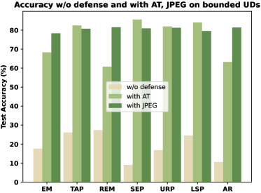
(a) Defense against seven SOTA bounded UDs.

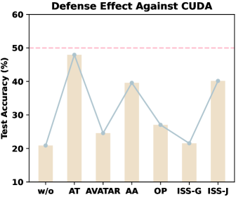
(b) Defense against CUDA with SOTA defenses.

Figure 1: (a) Using AT and JPEG is enough to effectively defend against so many SOTA bounded UDs. (b) Using existing SOTA defense schemes is powerless against CUDA. The accuracy results of Fig. 1 (a) (using ResNet18), and (b) (using ResNet50) are obtained on the CIFAR-10 dataset using SGD with a momentum of 0.9, a learning rate of 0.1, and a batch size of 128 for training 80 epochs. The compression factor of JPEG is set to 10 as suggested by Liu et al. (2023b).

Given this context, there is an urgent need to formulate a defense paradigm against the convolution-based UDs to tackle the challenges at hand. For designing a custom defense against convolution-based UDs, we first align with Min et al. (2021); Javanmard & Soltanolkotabi (2022) in simplifying the image samples as column vectors generated by a Gaussian mixture model (GMM) (Reynolds et al., 2009). In this manner, existing convolution-based unlearnable samples can be expressed as the product of a matrix and clean samples. This multiplicative matrix can be understood as multiplicative perturbations, in contrast to the additive perturbations in most bounded UDs.

Meanwhile, Sadasivan et al. (2023) find that the test accuracy breathtakingly surpasses 90% when adding universal multiplicative noise to the dataset, which implies that it is not the multiplicative noise itself that renders the dataset unlearnable. Hence, the reasons behind the effectiveness of convolution-based UDs remain to be further investigated. Inspired by the proposition from Yu et al. (2022) that the linearity separability property of noise is the reason for the effectiveness of UDs, we conjecture that either increasing the inconsistency within intra-class multiplicative noise or enhancing the similarity within inter-class multiplicative noise can both impair unlearnable effects. Back to the previously mentioned scenario with perfect multiplicative expression of unlearnable samples, we first formally define these two metrics as $\Theta_{imi}$ and $\Theta_{imc}$ customized for convolution-based UDs. Then we conduct validation experiments based on these two quantitative indicators, consequently supporting our hypothesis. Now we are just motivated to design a transformation technique for the multiplicative matrix to effectively boost $\Theta_{imi}$ and $\Theta_{imc}$, and then extend this technique to defend against real unlearnable images. Specifically, we leverage a uniform distribution to generate random values and random shifts to construct a new random matrix, which is universally applied to left-multiply unlearnable samples. This transformation simultaneously achieves an enhancement in both $\Theta_{imi}$ and $\Theta_{imc}$, subsequently improving the test accuracy.

By expanding this random matrix to high-dimensional real convolution-based unlearnable samples, we first propose COIN, a newly designed defense strategy for countering convolution-based UDs, employing randomly multiplicative image transformation as its mechanism. Concretely, we first sample random variables $\omega$ and $m$ from a uniform distribution. Afterwards, $m$ is used to obtain random pixels from unlearnable images for interpolation, and then we convert unlearnable samples to new samples via bilinear interpolation, involving $\omega$ for randomness. Extensive experiments reveal that our approach significantly overwhelms existing defense schemes, ranging from 19.17%-44.63% in test accuracy on CIFAR-10 and CIFAR-100. In addition, we replace the convolution kernels in CUDA with horizontal convolution filters and vertical convolution filters respectively to generate two new types of convolution-based UDs, namely VUDA and HUDA as shown in Fig. 2. In Section 5.4, we demonstrate that existing defenses are ineffective against VUDA and HUDA, however, our proposed defense COIN proves to be the most effective solution against these convolution-based UDs. Our contributions are summarized as:

• We are the first to focus on defenses against convolution-based UDs and the first to propose two brand-new metrics $\Theta_{imi}$ and $\Theta_{imc}$ tailored for convolution-based UDs to explore the underlying mechanism of them.

• To the best of our knowledge, we propose the first highly effective defense strategy against convolution-based UDs, termed as COIN, which utilizes a random pixel-based transformation and serves as a vital complement to the community of defense efforts against UDs.

• We further propose two new types of convolution-based UDs, i.e., VUDA, HUDA, and have demonstrated that our defense scheme COIN is the most effective against them.

• Extensive experiments against convolution-based UDs on three benchmark datasets and six commonly-used model architectures validate the effectiveness of our defense strategy.

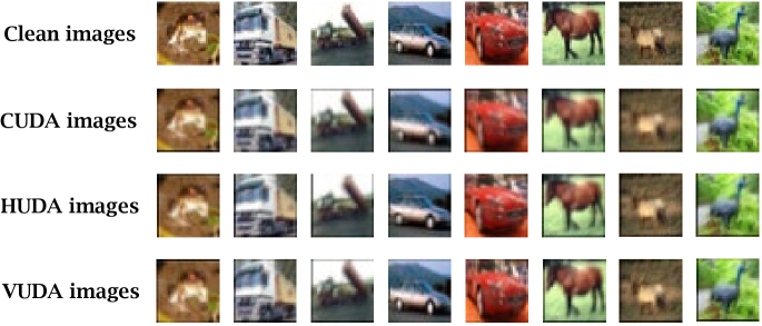
Figure 2: Visual representations of clean CIFAR-10 images and images from three types of convolution-based UDs, i.e., CUDA UD (Sadasivan et al., 2023), and two new convolution-based UDs (HUDA, VUDA) crafted by our own design.

2 Related Work

2.1 Unlearnable Datasets

Current unlearnable datasets can be classified into two categories, i.e., bounded UDs and convolution-based UDs. The methods for crafting bounded UDs are as follows: Huang et al. (2021) first introduce the concept of “unlearnable examples” and utilize a dual minimization optimization approach to generate additive unlearnable noise with a restricted range. Subsequently, generation methods based on targeted adversarial samples (Fowl et al., 2021), universal random noise (Tao et al., 2021), robust unlearnable examples (Fu et al., 2022), linearly separable perturbations (Yu et al., 2022), autoregressive processes (Sandoval-Segura et al., 2022b), one-pixel shortcut (Wu et al., 2023), and self-ensemble checkpoints (Chen et al., 2023) are successively proposed. Nonetheless, recent studies have indicated that popularly used defense techniques like AT and JPEG compression can readily counteract existing bounded UDs (Tao et al., 2021; Liu et al., 2023b).

Recently, a new type of convolution-based UDs have been newly proposed, i.e., Sadasivan et al. (2023) employ multiplicative convolutional operations to generate multiplicative noise without norm constraints. Unfortunately, all currently available defense methods prove ineffective against it, and there is currently no research exploring viable defense strategies.

2.2 Defenses Against UDs

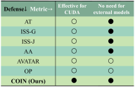
Figure 3: The defense effectiveness against CUDA and dependence on external models are presented. “$\bullet$” denotes fully satisfying the condition.

There are many defense techniques proposed for UDs so far. Tao et al. (2021) experimentally and theoretically demonstrate AT can effectively defend against bounded UDs, and Liu et al. (2023b) discover that simple image transformation techniques, i.e., grayscale transformation (a.k.a., ISS-G), and JPEG compression can also effectively defend against UDs. Thereafter, Qin et al. (2023b) employ adversarial augmentations (AA), Dolatabadi et al. (2023) purify UDs through diffusion models (AVATAR), while Segura et al. (2023) train a linear regression model to perform orthogonal projection (OP) on unlearnable samples. Nevertheless, none of these defense methods are tailor-made for convolution-based UDs, with all of them failing against CUDA (Sadasivan et al., 2023). In contrast, our proposed defense is specifically designed for convolution-based UDs, which effectively safeguards against existing convolution-based UD CUDA, offering a viable solution to the current vulnerability of security threats brought by convolution-based UDs. A detailed comparison of defense schemes can be found in Fig. 3.

3 Explaining the Mechanism of convolution-based UDs

3.1 Threat Model

The attacker creates a convolution-based unlearnable dataset by employing the convolutional kernel $\mathcal{K}_{i}$ to each image $x_{i}$ in the training set $\mathcal{D}_{c}$, thus causing the model $F$ with parameter $\theta$ trained on this dataset to generalize poorly to a clean test distribution $\mathcal{D}$ (Huang et al., 2021; Fowl et al., 2021; Yu et al., 2022; Sandoval-Segura et al., 2022b; Chen et al., 2023; Sadasivan et al., 2023; Wu et al., 2023). Formally, the attacker expects to work out the following bi-level objective:

$$\centering\max\underset{(x,y)\sim\mathcal{D}}{\mathbb{E}}\left[\mathcal{L}\left(F\left(x;\theta_{p}\right),y\right)\right]\@add@centering$$ (1)

$$\text{ {s.t.} }\theta_{p}=\underset{\theta}{\arg\min}\sum_{\left(x_{i},y_{i}\right)\in\mathcal{D}_{c}}\mathcal{L}\left(F\left(x_{i}\otimes\mathcal{K}_{i};\theta\right),y_{i}\right)$$ (2)

where $(x_{i},y_{i})$ represents the clean data from $\mathcal{D}_{c}$, $\mathcal{L}$ is a loss function, e.g., cross-entropy loss, and $\otimes$ represents the convolution operation, while ensuring the modifications to $x_{i}$ are not excessive for preserving the concealment of the sample.

As for defenders, in the absence of any knowledge of clean samples $x_{i}$, they aim to perform certain operations on UDs to achieve the opposite goal of Eq. 1.

3.2 Challenges

Yu et al. (2022) reveal that the effectiveness of bounded UDs can be attributed to the linear separability of additive noise. However, Segura et al. (2023) discover that not all bounded UDs exhibit this property, providing a counterexample (Sandoval-Segura et al., 2022b). Consequently, there is still no clear consensus on how bounded UDs are effective. More importantly, there are significant differences in the form of the noise between convolution-based UDs and bounded UDs, e.g., class-wise convolution-based perturbations from CUDA (Sadasivan et al., 2023) within the same class yet show non-identical noise, as illustrated in Fig. 10. This implies that the properties satisfied by the multiplicative noise corresponding to convolution-based UDs may be different from those of bounded UDs. Therefore, we are motivated to design custom evaluation metrics for assessing the “multiplication linearity separability” properties of convolution-based UDs, aiming to investigate the reasons behind the effectiveness of this new type of UDs.

3.3 Preliminaries

Similar to Min et al. (2021); Javanmard & Soltanolkotabi (2022), we define a binary classification problem involving a Bayesian classifier (Friedman et al., 1997), and the clean dataset $\mathcal{D}_{c}$ is sampled from a Gaussian mixture model $\mathcal{N}(y\bm{\mu},I)$. Here, $y$ represents the labels $\{\pm 1\}$, with mean $\bm{\mu}\in\mathbb{R}^{d}$, and covariance $I\in\mathbb{R}^{d\times d}$ as the identity matrix ($d$ represents the feature dimension). We denote the clean sample as $x\in\mathbb{R}^{d}$, the convolution-based unlearnable example $x_{u}$ in CUDA can be formulated as left-multiplying the class-wise matrices $\mathcal{A}(a_{y})$ by $x$, formulated as:

$$x_{u}=\mathcal{A}(a_{y})\cdot x$$ (3)

where $a_{y}$ is a parameter used to create a multiplicative matrix $\mathcal{A}$ (i.e., multiplicative noise) with respect to label $y$. Specifically, CUDA employs a tridiagonal matrix $\mathcal{A}_{c}\left(a_{y}\right)$, characterized by diagonal elements equal to 1, with the lower and upper diagonal elements set to $a_{y}$. The more intuitive forms of these matrices are provided in the Section A.1.1.

3.4 Hypothesis and Validations

Definition 1: We define the intra-class matrix inconsistency, denoted as $\Theta_{imi}$, as follows: Given the multiplicative matrices $\{\mathcal{A}_{i}\mid i=1,2,\cdots,n\}$ within a certain class $y_{k}$ (containing $n$ samples), we have an intra-class average matrix defined as ${\mathcal{A}_{\mu}}_{k}=\frac{1}{n}{\textstyle\sum_{i=1}^{n}}\mathcal{A}_{i}$, an intra-class matrix variance defined as $\mathbb{D}_{k}=\frac{1}{n}{\textstyle\sum_{i=1}^{n}}(\mathcal{A}_{i}-{\mathcal{A}_{\mu}}_{k})^{2}\in\mathbb{R}^{d\times d}$, an intra-class matrix variance mean value defined as ${\mathcal{V}_{m}}_{k}=\frac{1}{d^{2}}\sum_{i=0}^{d-1}\sum_{j=0}^{d-1}\mathbb{D}_{k}\left[i\right]\left[j\right]$, and then we have $\Theta_{imi}=\frac{1}{c}\sum_{k=0}^{c-1}{\mathcal{V}_{m}}_{k}$, where $c$ denotes the number of classes in $\mathcal{D}_{c}$.

Definition 2: We define the inter-class matrix consistency, denoted as $\Theta_{imc}$, as follows: Given the flattened intra-class average matrices of the j-th and k-th classes $flat({\mathcal{A}_{\mu}}_{j})$, $flat({\mathcal{A}_{\mu}}_{k})$, we then have $\Theta_{imc}=sim(flat({\mathcal{A}_{\mu}}_{j}),flat({\mathcal{A}_{\mu}}_{k}))$, where $flat\left(\right)$ denotes flattening the matrix into a row vector and $sim(\cdot,\cdot)$ denotes cosine similarity, i.e., $sim(u,v)=uv^{T}/(\left\|u\right\|\left\|v\right\|)$.

Inspired by the linear separability of additive noise in most bounded UDs, our intuition is that by decreasing the consistency of intra-class multiplicative matrices or increasing the consistency of inter-class multiplicative matrices, we can make the noise information introduced by the matrices more disordered and then less susceptible to be captured. This leads to classifiers failing to learn information unrelated to image features, thus resulting in an increase in test accuracy. In light of this, we propose our hypothesis as follows:

Hypothesis 1: When $a_{y}$ in the multiplicative matrix is within a reasonable range, increasing $\Theta_{imi}$ or $\Theta_{imc}$ can both improve the test accuracy of classifiers trained on convolution-based UDs, and vice versa.

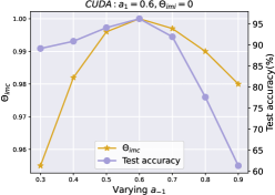
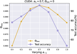
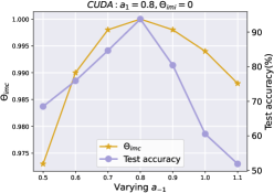
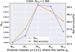
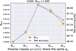
Figure 4: We explore the impact of $\Theta_{imc}$ (top row) and $\Theta_{imi}$ (bottom row) on test accuracy by manipulating the parameter $a_{y}$ in the process of generating CUDA datasets.

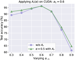
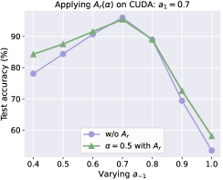
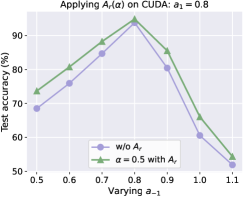
Figure 5: Comparison results of test accuracy before and after left-multiplying a random matrix $\mathcal{A}_{r}(\alpha)$ on all CUDA samples. $\alpha$ is all set to 0.5.

Validation: We first conduct experiments based on the preliminaries in Section 3.3 to construct CUDA datasets to validate our hypothesis. It can be observed from the top row of Fig. 4 that when $\Theta_{imi}$ remains constant, an increase in $\Theta_{imc}$ corresponds to an improvement in test accuracy, whereas a decrease in $\Theta_{imc}$ leads to a decline in test accuracy, i.e., $\Theta_{imc}$ and test accuracy exhibit the same trend of change. On the other hand, in the bottom row of Fig. 4, when $\Theta_{imc}$ is held constant, test accuracy increases as $\Theta_{imi}$ rises and decreases as $\Theta_{imi}$ falls. Hence, these experimental phenomena strongly support our proposed hypothesis. Additionally, we further explore in the top row Fig. 4, it is worth noting that when $\Theta_{imc}$=1.000 (i.e., $a_{1}$ equals $a_{-1}$), it is equivalent to multiplying all clean samples by the same matrix $\mathcal{A}_{c}$, which obtains high test accuracy results of exceeding 90% regardless of $a_{y}$ equals 0.6, 0.7, or 0.8. The implementation details of these plots and the specific values of matrix lists $a_{L_{1}}$-$a_{L_{15}}$ are provided in Section A.3.

3.5 Our design: Random Matrix $\mathcal{A}_{r}$

Based on the hypothesis and supporting experimental results mentioned above, we are motivated to find a method that perturbs the distributions of multiplicative matrix $\mathcal{A}(a_{y})$ in convolution-based UDs for increasing $\Theta_{imi}$ and $\Theta_{imc}$, thereby improving test accuracy to achieve defense effect.

Our intuition is to further left-multiply $\mathcal{A}(a_{y})$ by a random matrix $\mathcal{A}_{r}\in\mathbb{R}^{d\times d}$ to disrupt the matrix distribution. Concretely, to introduce randomness to the diagonal matrix $\mathcal{A}(a_{y})$ for increasing $\Theta_{imi}$, we first set random values filled with the diagonal of $\mathcal{A}_{r}$. However, the form of $\mathcal{A}(a_{y})$ remains unchanged by multiplying this $\mathcal{A}_{r}$, thus limiting the introduced randomness. Therefore, we add another set of random variables above the diagonal, but $\mathcal{A}_{c}$ still maintains the tridiagonal matrix structure. Thus, we shift variables by $m_{i}$ units simultaneously for each row to further enhance randomness. Due to the space limitation, more specific details regarding the above design reason on $\mathcal{A}_{r}$ are given in Section A.1.2. Next, we unify the random values and random shifts mentioned above using a uniform distribution $\mathcal{U}(-\alpha,\alpha)$, and ensure that the $\alpha$ is consistent for each class, thereby striving to enhance $\Theta_{imc}$ as much as possible while already improving $\Theta_{imi}$. During matrix $\mathcal{A}_{r}$ creation process, we first sample a variable $s\sim\mathcal{U}(-\alpha,\alpha,size=d),s\in\mathbb{R}^{d}$, and then obtain $m_{i}=\left\lfloor s_{i}\right\rfloor,n_{i}=s_{i}-m_{i},0\leq i\leq d-1$. The random matrix $\mathcal{A}_{r}$ is parameterized by $\alpha$ and is designed as:

$$\mathcal{A}_{r}(\alpha)=\begin{bmatrix}&\underline{1-n_{0}}&\underline{n_{0}}&0&0&\dots&0\\ &0&\underline{1-n_{1}}&\underline{n_{1}}&0&\dots&0\\ &0&0&\underline{1-n_{2}}&\underline{n_{2}}&\dots&0\\ &\vdots&\vdots&\vdots&\ddots&\vdots&\vdots\\ &\vdots&\vdots&\vdots&\vdots&\ddots&\vdots\\ &0&\dots&\dots&\dots&0&\underline{1-n_{d-1}}\end{bmatrix}\in\mathbb{R}^{d\times d}$$ (4)

where the $i$-th and ($i$+1)-th elements of the $i$-th row (0$\leq i\leq d$-1) are $1-n_{i}$ and $n_{i}$, and “$\underline{1-n_{i}},\underline{n_{i}}$” means that the positions of these two elements for each row are shifted by $m_{i}$ units simultaneously. When the new location $i+m_{i}$ or $i+1+m_{i}$ exceeds the matrix boundaries, we take its modulus with respect to $d$ to obtain the new position. The implementation process of the $\mathcal{A}_{r}(\alpha)$ can be found in Algorithm 1.

Whereupon, we obtain test accuracy by left-multiplying all CUDA samples with a random matrix $\mathcal{A}_{r}(\alpha)$, and then compare it with training on the CUDA UD without $\mathcal{A}_{r}(\alpha)$. Firstly, both $\Theta_{imi}$ and $\Theta_{imc}$ increase indeed when $\mathcal{A}_{r}(\alpha)$ is employed as demonstrated in Tables 5, 6 and 7. Secondly, we observe that the test accuracy with employing $\mathcal{A}_{r}$ is ahead of the accuracy obtained without using $\mathcal{A}_{r}$ regardless of $a_{1}$ is set to 0.6, 0.7, or 0.8 , as shown in Fig. 5, which is also consistent with our hypothesis. Ablation experiments on parameter $\alpha$ in $\mathcal{A}_{r}$ are in Section A.4.

4 Methodology

4.1 Our Design for Defense Scheme COIN

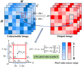
Figure 6: Our defense scheme COIN.

Inspired by the linear interpolation process (Blu et al., 2004), we find that the two random values in each row of $\mathcal{A}_{r}$ can be effectively modeled as two weighting coefficients, and the random location offset $m_{i}$ in each row can be directly exploited to find the positions for interpolation. Therefore, the previous process of left-multiplying the matrix $\mathcal{A}_{r}$ can be modeled as a random linear interpolation process to be applied for image transformations. In view of this, we are able to directly extend random matrix $\mathcal{A}_{r}$ to be employed in real image domain. Unlike the previous sample $x\in\mathbb{R}^{d}$, the unlearnable image $x_{u}\in\mathbb{R}^{C\times H\times W}$ requires variables along with both horizontal and vertical directions and employing bilinear interpolation instead of linear interpolation. The formulaic definitions are as follows:

$$s_{x},s_{y}\sim\mathcal{U}(-\alpha,\alpha,size=H\cdot W)$$ (5)

where $\mathcal{U}$ denotes a uniform distribution with size of height $H$ multiplied by width $W$, $\alpha$ controls the range of the generated random variables. Considering that $s_{x}$ and $s_{y}$ are both fundamentally arrays with size of $H\cdot W$, we obtain arrays $m_{x}$ and $m_{y}$ by rounding down each variable from the arrays to its integer part (i.e., random location offsets), formulated as follows:

$${m_{x}}_{i}=\left\lfloor{s_{x}}_{i}\right\rfloor,\quad{m_{y}}_{i}=\left\lfloor{s_{y}}_{i}\right\rfloor$$ (6)

where $\lfloor$ $\rfloor$ represents the floor function, and $i$ is the index in the array, ranging from $0$ to $H\cdot W-1$ (with the same meaning in the equations below). Subsequently, the arrays with coefficients required for interpolation $\omega_{x}$, $\omega_{y}$ are computed as follows:

$${\omega_{x}}_{i}={s_{x}}_{i}-{m_{x}}_{i},\quad{\omega_{y}}_{i}={s_{x}}_{i}-{m_{y}}_{i}$$ (7)

To obtain the coordinates of the pixels used for interpolation, we first initialize a coordinate grid:

$$c_{x},c_{y}=meshgrid(arange(W),arange(H))\in\mathbb{R}^{H\times W}$$ (8)

where $meshgrid$ denotes coordinate grid creation function, $arange$ is employed to produce an array with values evenly distributed within a specified range. So now we can obtain the coordinates of the four nearest pixel points around the desired interpolation point in the bilinear interpolation process:

$${q_{11}}_{i}=(({c_{x}}_{i}+{m_{x}}_{i})\%W,({c_{y}}_{i}+{m_{y}}_{i})\%H)$$ (9)

$${q_{21}}_{i}=(({c_{x}}_{i}+{m_{x}}_{i}+1)\%W,({c_{y}}_{i}+{m_{y}}_{i})\%H)$$ (10)

$${q_{12}}_{i}=(({c_{x}}_{i}+{m_{x}}_{i})\%W,({c_{y}}_{i}+{m_{y}}_{i}+1)\%H)$$ (11)

$${q_{22}}_{i}=(({c_{x}}_{i}+{m_{x}}_{i}+1)\%W,({c_{y}}_{i}+{m_{y}}_{i}+1)\%H)$$ (12)

where $\%$ represents the modulo function, ensuring that the horizontal coordinate ranges from 0 to $W-1$ and the vertical coordinate ranges from 0 to $H-1$. Hence, we obtain new pixel values by using the pixel values of the four points mentioned above through bilinear interpolation:

$$\mathcal{F}_{j}({p}_{i})=\begin{bmatrix}{1-\omega_{x}}_{i}&{\omega_{x}}_{i}\\ \end{bmatrix}\begin{bmatrix}\mathcal{F}_{j}({q_{11}}_{i})&\mathcal{F}_{j}({q_{12}}_{i})\\ \mathcal{F}_{j}({q_{21}}_{i})&\mathcal{F}_{j}({q_{22}}_{i})\end{bmatrix}\begin{bmatrix}{1-\omega_{y}}_{i}\\ {\omega_{y}}_{i}\end{bmatrix}$$ (13)

where $\mathcal{F}_{j}()$ denotes the pixel value of the $j$-th channel at a certain coordinate point, $p_{i}$ denotes the coordinate of the newly generated pixel point. Each generated pixel value should be clipped within the range (0,1). Finally, we gain the transformed image $x_{t}$ by applying Eq. 13 and clipping to pixel values of each channel of the image $x_{u}$. The schematic diagram of the above process is shown in Fig. 6, and we summarize the complete process in Algorithm 2.

4.2 Our Design for New Convolution-based UDs

To validate that our defense solution is effective against convolution-based UDs and not solely limited to CUDA, we have newly designed two convolution-based UDs, namely HUDA and VUDA. In particular, HUDA utilizes class-wise horizontal filters to generate UDs. The definition of its convolutional kernel is as follows:

$$\omega_{i,j,k,l}=\begin{cases}b_{y}&\text{ if }j=\frac{\mathcal{S}}{2}\quad and\quad i\in\{0,1,2\}\\ 0&\text{else}\end{cases}$$ (14)

where $i$ represents the channel, $j$ and $k$ denote the rows and columns of the convolutional kernel, and $l$ represents the depth of the convolutional kernel, $\mathcal{S}$ denotes the kernel size, and $b_{y}$ denotes the class-wise blur parameter. Similarly, the definition of the vertical convolutional kernel of VUDA scheme is as shown:

$$\omega_{i,j,k,l}=\begin{cases}b_{y}&\text{ if }k=\frac{\mathcal{S}}{2}\quad and\quad i\in\{0,1,2\}\\ 0&\text{else}\end{cases}$$ (15)

After obtaining the class-wise convolutional kernels, the entire dataset is processed using convolution operations to obtain the convolution-based UDs.

5 Experiments

5.1 Experimental Settings

Four widely-used network architectures including ResNet (RN) (He et al., 2016), DenseNet (DN) (Huang et al., 2017), MobileNetV2 (MNV2) (Sandler et al., 2018), GoogleNet (GN) (Szegedy et al., 2015), InceptionNetV3 (INV3) (Szegedy et al., 2016), and VGG (Simonyan & Zisserman, 2014) are selected. Meanwhile, three benchmark datasets CIFAR-10 (Krizhevsky & Hinton, 2009), CIFAR-100 (Krizhevsky & Hinton, 2009), and ImageNet100 (Deng et al., 2009) are employed. The uniform distribution range $\alpha$ is set to 2.0. During training on existing convolution-based UDs, we use SGD for training for 80 epochs with a momentum of 0.9, a learning rate of 0.1, and batch sizes of 128, 32 for CIFAR dataset, ImageNet100 dataset, respectively.

Datasets	CIFAR-10 (Krizhevsky & Hinton, 2009)						CIFAR-100 (Krizhevsky & Hinton, 2009)				AVG
Defenses$\downarrow$     Models$\rightarrow$	RN18	VGG16	DN121	MNV2	GN	INV3	RN18	VGG16	DN121	MNV2
w/o	26.49	24.65	27.21	21.34	18.73	21.10	14.31	12.53	13.90	12.94	19.32
MU (Zhang et al., 2018)	26.72	28.07	24.67	24.63	26.04	24.99	17.09	13.35	19.97	13.55	21.91
CM (Yun et al., 2019)	26.02	28.53	24.64	20.73	20.11	24.25	12.51	10.14	20.77	10.14	19.78
CO (DeVries & Taylor, 2017)	20.07	27.58	24.86	20.46	18.87	26.06	12.80	10.56	16.19	13.56	19.10
DP-SGD (Hong et al., 2020)	25.50	23.02	25.25	25.78	17.65	21.18	12.42	10.56	16.36	12.72	19.04
AT (Tao et al., 2021)	50.59	45.95	49.01	42.59	50.62	47.66	37.27	28.18	34.21	35.74	42.18
AVATAR (Dolatabadi et al., 2023)	30.67	29.57	33.15	28.53	30.40	24.68	14.49	10.81	12.97	13.85	22.91
AA (Qin et al., 2023b)	39.85	38.68	38.92	41.06	38.58	39.01	24.83	1.00	27.89	20.49	31.03
OP (Segura et al., 2023)	29.77	30.33	33.82	28.86	26.52	23.94	20.17	14.59	15.55	23.02	24.66
ISS-G (Liu et al., 2023b)	25.77	21.42	26.73	19.85	15.41	22.63	8.80	6.40	11.48	8.71	16.72
ISS-J (Liu et al., 2023b)	45.10	40.26	39.79	41.46	38.49	41.49	33.62	26.92	28.94	31.23	36.73
COIN (Ours)	71.90	73.65	70.45	73.63	72.88	69.07	48.63	46.74	45.72	48.53	61.35

Table 1: Test accuracy (%) on CIFAR-10 and CIFAR-100 with defenses against CUDA.

5.2 Defense Competitors

Defenses$\downarrow$     Models$\rightarrow$	RN18	RN50	DN121	MNV2	AVG
w/o	25.74	26.66	21.70	16.30	22.60
MU (Zhang et al., 2018)	34.96	19.38	27.78	15.60	24.43
CM (Yun et al., 2019)	16.54	24.04	23.58	8.00	18.04
CO (DeVries & Taylor, 2017)	25.46	29.20	23.90	17.58	24.04
AT (Tao et al., 2021)	37.82	36.80	30.34	41.42	36.60
ISS-G (Liu et al., 2023b)	14.92	13.50	9.78	5.78	11.00
ISS-J (Liu et al., 2023b)	30.10	37.04	25.52	28.04	30.18
COIN (Ours)	37.80	35.38	35.22	41.50	37.48

Table 2: Test accuracy (%) on ImageNet with defenses against CUDA.

We compare our defense COIN with SOTA defenses against UDs, i.e., AT (Tao et al., 2021), ISS (Liu et al., 2023b) (including JPEG compression, a.k.a., ISS-J and grayscale transformation, a.k.a., ISS-G), AVATAR (Dolatabadi et al., 2023), OP (Segura et al., 2023), and AA (Qin et al., 2023b). We also apply four defense strategies proposed by Borgnia et al. (2021), i.e., differential privacy SGD (DP-SGD) (Hong et al., 2020; Zhang et al., 2021), cutmix (CM) (Yun et al., 2019), cutout (CO) (DeVries & Taylor, 2017), and mixup (MU) (Zhang et al., 2018), which are popularly used to test whether it can defend against UDs. Consistent with previous works (Liu et al., 2023b; Tao et al., 2021; Qin et al., 2023b), we evaluate defense schemes with test accuracy, i.e., the model accuracy on a clean test set after training on UDs.

5.3 Evaluation on Our Defense COIN

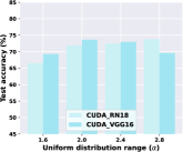
Figure 7: Using COIN against CUDA with varying $\alpha$ on RN18 and VGG16.

The test accuracy results for defense against existing convolution-based UDs on benchmark datasets are presented in Tables 1 and 2. “AVG” denotes the average value for each row. The values covered by deep green denote the best defense effect, while values covered by light green denote the second-best defense effect.

It can be observed the average test accuracy (i.e., values in AVG column) obtained by existing defense schemes against CUDA (Sadasivan et al., 2023) lag behind COIN by as much as 19.17%-44.63% as shown in Table 1, which demonstrates the superiority of our defense. Meanwhile, our defense scheme also maintains a leading advantage of 0.88%-26.48% on large datasets as shown in Table 2. The reason ISS-J largely lags behind COIN against CUDA can be deduced from Fig. 10, i.e., the excessive global multiplicative noise introduced by CUDA results in a significant loss of features after the lossy compression from ISS-J. Additional explorations in COIN against bounded UDs are demonstrated in Section A.5.

5.4 Evaluation on Other Types of Convolution-based UDs

Datasets	VUDA CIFAR-10					HUDA CIFAR-10
Defenses$\downarrow$     Models$\rightarrow$	RN18	VGG16	DN121	MNV2	AVG	RN18	VGG16	DN121	MNV2	AVG
w/o	40.36	43.95	44.03	36.86	41.30	39.65	36.63	50.32	34.73	40.53
MU (Zhang et al., 2018)	41.13	41.66	39.98	39.55	40.58	43.45	44.54	48.96	42.01	43.91
CM (Yun et al., 2019)	42.15	37.71	39.62	37.95	39.36	38.56	39.68	50.38	41.37	41.87
CO (DeVries & Taylor, 2017)	39.93	38.95	36.64	38.37	38.47	40.53	40.18	47.74	36.58	40.70
DP-SGD (Hong et al., 2020)	39.39	41.01	46.04	37.26	40.93	36.76	41.08	46.34	35.75	40.17
AT (Tao et al., 2021)	43.40	38.68	46.88	36.33	41.32	48.62	41.19	50.48	43.74	45.07
AA (Qin et al., 2023b)	51.87	10.00	60.09	51.42	43.35	56.83	10.00	60.09	61.08	46.27
OP (Segura et al., 2023)	42.67	39.26	46.25	41.04	42.31	45.36	46.77	59.80	51.79	49.21
ISS-G (Liu et al., 2023b)	38.50	32.88	38.46	33.66	35.88	22.43	43.08	29.33	34.52	33.05
ISS-J (Liu et al., 2023b)	51.49	45.00	45.54	38.57	45.15	49.89	49.48	42.23	40.58	45.47
COIN (Ours)	74.98	68.74	74.96	71.07	72.44	75.18	71.75	75.78	70.10	73.05

Table 3: Test accuracy (%) on CIFAR-10 with defenses against two new types of convolution-based UDs VUDA and HUDA.

We compare our defense COIN with other state-of-the-art defenses against VUDA and HUDA UDs, and the defense results are shown in Table 3. It can be observed that our defense is effective in defending against these new types of convolution-based UDs and performs significantly better than other defense solutions by 23.84% to 40%. These results further highlight the vulnerability of existing defense solutions to newly emerging convolution-based UDs. On the other hand, our proposed defense COIN effectively addresses this gap.

5.5 Ablation Experiments on $\alpha$

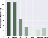
Figure 8: Time overhead on CIFAR-10 using RN18.

We investigate the impact of uniform distribution range $\alpha$ on the effectiveness of our defense COIN, as shown in Fig. 7. The test accuracy against CUDA increases initially with the rise in $\alpha$ and then starts to decrease. This is because initially, as $\alpha$ increases, the CUDA perturbations gradually become disrupted. However, as $\alpha$ continues to increase, excessive corruptions damage image features, leading to a deterioration in defense effect. We opt for an $\alpha$ of 2.0 that yields the highest average defense effect.

5.6 Time complexity analysis for COIN

Assuming that the time complexity of each line of code in Algorithm 2 is $\mathcal{O}(1)$, then for an convolution-based UD $\mathcal{D}_{u}=\{{x_{u}}_{i}\in\mathbb{R}^{C\times H\times W}\}_{i=1}^{N}$, the overall time complexity of performing COIN is $\mathcal{O}(N\times C\times H\times W)+\mathcal{O}(N\times H\times W)+\mathcal{O}(N)$. Due to the fact that the values of $C$, $H$, and $W$ of image ${x_{u}}_{i}$ are constant, e.g., $C$=3, $H$=32, and $W$=32 for CIFAR-10 images, the final time complexity is optimized to: $\mathcal{O}(N)+\mathcal{O}(N)+\mathcal{O}(N)=\mathcal{O}(N)$. We then employ multiple defense strategies when training ResNet18 on CUDA CIFAR-10 for 80 epochs, and measure their corresponding time overheads, as shown in Fig. 8. We can conclude that our defense approach COIN is relatively efficient compared with existing defense schemes.

6 Conclusion

In this paper, we demonstrate for the first time that existing defense mechanisms against UDs are all ineffective against convolution-based UDs. In light of this, we focus for the first time the challenging issue of defending against convolution-based UDs. Subsequently, we model the process of existing convolution-based UDs based on GMMs and Bayesian binary problems by applying multiplicative matrices to samples. Simultaneously, we discover that the consistency of intra-class and inter-class noise in convolution-based UDs has a profound impact on the unlearnable effect, then we define two quantitative metrics $\Theta_{imi}$ and $\Theta_{imc}$ and investigate how to mitigate the impact of multiplicative matrices. We find increasing both of these two metrics can mitigate the effectiveness of convolution-based UDs and design a new random matrix to increase both metrics. Furthermore, in the context of real samples and based on the above ideas, we first propose a novel image transformation based on global pixel-level random resampling via bilinear interpolation, which universally guards against existing convolution-based UDs. In addition, we have newly designed two different types of convolution-based UDs and experimentally validated the effectiveness of our defense approach against all of them. Extensive experiments on various benchmark datasets and widely-used models verified the effectiveness of our defense.

Appendix A Appendix

A.1 Intuitive displays of Matrices

A.1.1 Intuitive displays of $\mathcal{A}(a_{y})$ and $\mathcal{A}_{r}(\alpha)$

During CUDA UDs (Sadasivan et al., 2023) generation process, the tridiagonal matrix $\mathcal{A}_{c}\left(a_{y}\right)$ is designed as:

$$\mathcal{A}_{c}\left(a_{y}\right)=\left[\begin{array}[]{cccccc}1&a_{y}&0&0&\ldots&0\\ a_{y}&1&a_{y}&0&\ldots&0\\ 0&a_{y}&1&a_{y}&\ldots&\vdots\\ \vdots&\vdots&\vdots&\ddots&\ddots&0\\ \vdots&\vdots&\vdots&\vdots&\ddots&a_{y}\\ 0&\ldots&\ldots&0&a_{y}&1\end{array}\right]\in\mathbb{R}^{d\times d}$$ (16)

where constant $a_{y}$ corresponding to different $y$ is also different.

As for our newly designed upper triangular matrix, which is defined as:

$$\mathcal{A}_{u}\left(a_{y}\right)=\left[\begin{array}[]{cccccc}1&a_{y}&0&0&\ldots&0\\ 0&1&a_{y}&0&\ldots&0\\ 0&0&1&a_{y}&\ldots&\vdots\\ \vdots&\vdots&\vdots&\ddots&\ddots&0\\ \vdots&\vdots&\vdots&\vdots&\ddots&a_{y}\\ 0&\ldots&\ldots&0&0&1\end{array}\right]\in\mathbb{R}^{d\times d}$$ (17)

where constant $a_{y}$ corresponding to different $y$ is also different. Similarly, the lower triangular matrix is defined as:

$$\mathcal{A}_{l}\left(a_{y}\right)=\left[\begin{array}[]{cccccc}1&0&0&0&\ldots&0\\ a_{y}&1&0&0&\ldots&0\\ 0&a_{y}&1&0&\ldots&\vdots\\ \vdots&\vdots&\vdots&\ddots&\ddots&0\\ \vdots&\vdots&\vdots&\vdots&\ddots&0\\ 0&\ldots&\ldots&0&a_{y}&1\end{array}\right]\in\mathbb{R}^{d\times d}$$ (18)

where constant $a_{y}$ corresponding to different $y$ is also different.

During matrix $\mathcal{A}_{r}$ creation process, we first sample a variable $s\sim\mathcal{U}(-\alpha,\alpha,size=d),s\in\mathbb{R}^{d}$, and then obtain $m_{i}=\left\lfloor s_{i}\right\rfloor,n_{i}=s_{i}-m_{i},0\leq i\leq d-1$. The random matrix $\mathcal{A}_{r}$ is parameterized by $\alpha$ and is designed as:

$$\mathcal{A}_{r}(\alpha)=\begin{bmatrix}&\underline{1-n_{0}}&\underline{n_{0}}&0&0&\dots&0\\ &0&\underline{1-n_{1}}&\underline{n_{1}}&0&\dots&0\\ &0&0&\underline{1-n_{2}}&\underline{n_{2}}&\dots&0\\ &\vdots&\vdots&\vdots&\ddots&\vdots&\vdots\\ &\vdots&\vdots&\vdots&\vdots&\ddots&\vdots\\ &0&\dots&\dots&\dots&0&\underline{1-n_{d-1}}\end{bmatrix}\in\mathbb{R}^{d\times d}$$ (19)

where the $i$-th and ($i$+1)-th elements of the $i$-th row (0$\leq i\leq d$-1) are $1-n_{i}$ and $n_{i}$, and “$\underline{1-n_{i}},\underline{n_{i}}$” means that the positions of these two elements for each row are shifted by $m_{i}$ units simultaneously. When the new location $i+m_{i}$ or $i+1+m_{i}$ exceeds the matrix boundaries, we take its modulus with respect to $d$ to obtain the new position. The detailed process can be referred to in Algorithm 1.

Input : Feature dimension $d$; matrix strength $\alpha$.

Output : Matrix $\mathcal{A}_{r}(\alpha)$.

Function : Uniform distribution $\mathcal{U}$.

1

2Randomly sample $s=\mathcal{U}(-\alpha,\alpha,size=d)$;

3Round down to the integer $m=\left\lfloor s\right\rfloor$;

4Fractional part $n=s-m$;

5Initialize a matrix with all zeros $\mathcal{A}_{r}(\alpha)\in\mathbb{R}^{d\times d}$;

6for $i$ = 0 to ($d-1$) do

7       for $j$ = 0 to ($d-1$) do

8             if $i+m[i]<0$ then

9                   $x=i+m[i]+d-1$;

10             end if

11            else if $i+m[i]>d-1$ then

12                   $x=i+m[i]-d+1$;

13             end if

14            else

15                   $x=i+m[i]$;

16             end if

17            if $x==j$ then

18                   $\mathcal{A}_{r}(\alpha)[i,j]=1-n[i]$;

19             end if

20            else if $(x+1)\%d==j$ then

21                   $\mathcal{A}_{r}(\alpha)[i,j]=n[i]$;

22             end if

23            

24       end for

25      

26 end for

Return: Matrix $\mathcal{A}_{r}(\alpha)$.

Algorithm 1 Matrix $\mathcal{A}_{r}(\alpha)$ creation process

A.1.2 Why do we design $\mathcal{A}_{r}$ like this?

We will explain the rationale behind the design of the $\mathcal{A}_{r}$ matrix. First of all, we define a diagonal matrix $\mathcal{A}_{o}$, which might be a new matrix representation of a potential convolution-based attack similar to bounded UD OPS (Wu et al., 2023), and a matrix $\mathcal{A}_{tr}$ with random values on its diagonal elements formulated as:

$$\mathcal{A}_{o}\left(a_{y},i\right)=\left[\begin{array}[]{cccccc}1&0&0&0&\ldots&0\\ 0&\ddots&0&0&\ldots&0\\ 0&0&1&0&\ldots&0\\ \vdots&\vdots&\vdots&a_{y}&\vdots&\vdots\\ \vdots&\vdots&\vdots&\vdots&1&\vdots\\ 0&\ldots&\ldots&0&0&1\end{array}\right]\in\mathbb{R}^{d\times d}$$ (20)

$$\mathcal{A}_{tr}=\left[\begin{array}[]{cccccc}n_{0}&0&0&0&\ldots&0\\ 0&n_{1}&0&0&\ldots&0\\ 0&0&\ddots&0&\ldots&0\\ \vdots&\vdots&\vdots&n_{i}&\vdots&\vdots\\ \vdots&\vdots&\vdots&\vdots&\ddots&\vdots\\ 0&\ldots&\ldots&0&0&n_{d-1}\end{array}\right]\in\mathbb{R}^{d\times d}$$ (21)

where $n_{0}$, $n_{1}$, …, $n_{d-1}$ are all random values. If we multiply matrix $\mathcal{A}_{tr}$ by $\mathcal{A}{(a_{y})}$, we will get new matrices as:

$$\mathcal{A}_{tr}\cdot\mathcal{A}_{c}(a_{y})=\left[\begin{array}[]{cccccc}n_{0}&n_{0}a_{y}&0&0&\ldots&0\\ n_{1}a_{y}&n_{1}&n_{1}a_{y}&0&\ldots&0\\ 0&\ddots&\ddots&\ddots&\ldots&0\\ \vdots&\vdots&n_{i}a_{y}&n_{i}&n_{i}a_{y}&\vdots\\ \vdots&\vdots&\vdots&\ddots&\ddots&\vdots\\ 0&\ldots&\ldots&0&n_{d-1}a_{y}&n_{d-1}\end{array}\right]\in\mathbb{R}^{d\times d}$$ (22)

$$\mathcal{A}_{tr}\cdot\mathcal{A}_{o}(a_{y})=\left[\begin{array}[]{cccccc}n_{0}&0&0&0&\ldots&0\\ 0&n_{1}&0&0&\ldots&0\\ 0&0&\ddots&0&\ldots&0\\ \vdots&\vdots&\vdots&n_{i}a_{y}&\vdots&\vdots\\ \vdots&\vdots&\vdots&\vdots&\ddots&\vdots\\ 0&\ldots&\ldots&0&0&n_{d-1}\end{array}\right]\in\mathbb{R}^{d\times d}$$ (23)

Apparently, setting random variables only on the diagonal like $\mathcal{A}_{tr}$ does not alter the original form of the multiplicative matrix, i.e., $\mathcal{A}_{c}$ remains a tridiagonal matrix, and $\mathcal{A}_{o}$ remains a diagonal matrix, which has a very limited effect on disrupting the distribution of the original matrix.

So, how would adding another set of random variables above the diagonal change the form of the matrix? Thus, we define a new matrix $\mathcal{A}_{sr}$ as:

$$\mathcal{A}_{sr}=\begin{bmatrix}&1-n_{0}&n_{0}&0&0&\dots&0\\ &0&1-n_{1}&n_{1}&0&\dots&0\\ &0&0&1-n_{2}&n_{2}&\dots&0\\ &\vdots&\vdots&\vdots&\ddots&\vdots&\vdots\\ &\vdots&\vdots&\vdots&\vdots&\ddots&\vdots\\ &0&\dots&\dots&\dots&0&1-n_{d-1}\end{bmatrix}\in\mathbb{R}^{d\times d}$$ (24)

where $n_{0}$, $n_{1}$, …, $n_{d-1}$ are all random values. Similarly, we multiply it with $\mathcal{A}(a_{y})$ to obtain the following result:

It can be observed that the matrix $\mathcal{A}_{o}$ has completely altered its form, accommodating more randomness. However, $\mathcal{A}_{c}$ still maintains the tridiagonal matrix form. So, in order to alter the form of $\mathcal{A}_{c}$ as much as possible for introducing as much randomness as possible, it seems reasonable to add another set of random values below the diagonal of $\mathcal{A}_{sr}$. However, this idea encounters two challenging practical issues: i@: Adding more diagonal values would significantly increase the computational cost of matrix multiplication, which is not conducive to efficient algorithms. ii@: More diagonal values correspond to more noise, which will harm sample features. Therefore, this way is not feasible. So, we come up with the idea of introducing small random offsets to the random variables for each row. This approach both does not introduce new variables also breaks the original tridiagonal form of the matrix $\mathcal{A}_{c}(a_{y})$, thus further increasing randomness.

A.2 Further Study on Image Corruptions

The defense strategy we propose, along with ISS-G and ISS-J, fundamentally fall within the domain of corruption techniques (Liu et al., 2023a; Hu et al., 2023; Zhou et al., 2023a; b). Hence, we aim to explore additional image corruption operations to ascertain the possibility of more potential defenses against convolution-based UDs, as illustrated in Fig. 9. It can be observed that the majority of these commonly used image corruptions are largely ineffective in defending against convolution-based UDs. Delving deeper into the defense against these image corruption techniques for convolution-based UDs would be a meaningful avenue for future research.

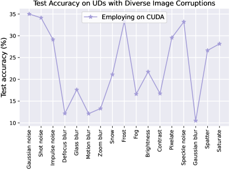
Figure 9: Test accuracy (%) on CIFAR-10 using RN18 with corruptions against CUDA.

Matrix list $a_{L_{i}}$	$a_{L_{1}}$	$a_{L_{2}}$	$a_{L_{3}}$	$a_{L_{4}}$	$a_{L_{5}}$
$a_{y}$ values in list	[0.4]	[0.2, 0.3, 0.4]	[0.03, 0.06, 0.1, 0.2, 0.3, 0.4]	[0.05, 0.1, 0.2, 0.3, 0.4]	[0.1, 0.2, 0.3, 0.4]
Matrix list $a_{L_{i}}$	$a_{L_{6}}$	$a_{L_{7}}$	$a_{L_{8}}$	$a_{L_{9}}$	$a_{L_{10}}$
$a_{y}$ values in list	[0.5]	[0.3, 0.5, 0.7]	[0.05, 0.1, 0.5, 0.7]	[0.1, 0.5, 0.7]	[0.2, 0.5, 0.7]
Matrix list $a_{L_{i}}$	$a_{L_{11}}$	$a_{L_{12}}$	$a_{L_{13}}$	$a_{L_{14}}$	$a_{L_{15}}$
$a_{y}$ values in list	[0.6]	[0.4, 0.6, 0.8]	[0.05, 0.1, 0.3, 0.6, 0.9]	[0.1, 0.2, 0.4, 0.6, 0.8, 0.9]	[0.2, 0.4, 0.6, 0.8]

Table 4: The specific values of the matrix lists ${a_{L}}_{1}$-${a_{L}}_{15}$ are shown. Each $a_{y}$ value corresponds to the matrix $\mathcal{A}_{c}(a_{y})$, and the matrix lists ${a_{L}}_{i}$ used for both classes are identical.

w/o $\mathcal{A}_{r}$, $a_{-1}\rightarrow$	0.3	0.4	0.5	0.6	0.7	0.8	0.9
$\Theta_{imi}$	0	0	0	0	0	0	0
$\Theta_{imc}$	0.955	0.982	0.996	1.000	0.997	0.990	0.980
$\mathcal{A}_{r}(0.5)$, $a_{-1}\rightarrow$	0.3	0.4	0.5	0.6	0.7	0.8	0.9
$\Theta_{imi}$	0.000664	0.000663	0.000674	0.000698	0.000738	0.000782	0.000845
$\Theta_{imc}$	0.981	0.993	0.998	1.000	0.999	0.996	0.992

Table 5: The specific values of $\Theta_{imi}$ and $\Theta_{imc}$ before and after using $\mathcal{A}_{r}$ on CUDA samples with $a_{1}=0.6$ and varying $a_{-1}$ in Fig. 5.

A.3 Implementation details of Validation experiments

Similar to CUDA (Sadasivan et al., 2023), we sample 1000 samples from the Gaussian Mixture Model (with $\left\|\bm{\mu}\right\|_{2}$=2.0, $d$=100) as described in Section 3.3, and evenly split them into a training set (used for generating new training sets by CUDA) and a test set. We train a Naive Bayes classifier on the new training set and then calculate the test accuracy on the test set with the trained classifier. The results of test accuracy reported in Section 3.4 are the average results obtained after running the experiments 10 times with diverse random seeds.

w/o $\mathcal{A}_{r}$, $a_{-1}\rightarrow$	0.4	0.5	0.6	0.7	0.8	0.9	1.0
$\Theta_{imi}$	0	0	0	0	0	0	0
$\Theta_{imc}$	0.965	0.986	0.997	1.000	0.998	0.992	0.985
$\mathcal{A}_{r}(0.5)$, $a_{-1}\rightarrow$	0.4	0.5	0.6	0.7	0.8	0.9	1.0
$\Theta_{imi}$	0.000701	0.000712	0.000734	0.000770	0.000822	0.000877	0.000953
$\Theta_{imc}$	0.986	0.994	0.999	1.000	0.999	0.997	0.994

Table 6: The specific values of $\Theta_{imi}$ and $\Theta_{imc}$ before and after using $\mathcal{A}_{r}$ on CUDA samples with $a_{1}=0.7$ and varying $a_{-1}$ in Fig. 5.

w/o $\mathcal{A}_{r}$, $a_{-1}\rightarrow$	0.5	0.6	0.7	0.8	0.9	1.0	1.1
$\Theta_{imi}$	0	0	0	0	0	0	0
$\Theta_{imc}$	0.973	0.990	0.998	1.000	0.998	0.994	0.988
$\mathcal{A}_{r}(0.5)$, $a_{-1}\rightarrow$	0.5	0.6	0.7	0.8	0.9	1.0	1.1
$\Theta_{imi}$	0.000762	0.000785	0.000818	0.000865	0.000929	0.000996	0.001083
$\Theta_{imc}$	0.989	0.996	0.999	1.000	0.999	0.997	0.995

Table 7: The specific values of $\Theta_{imi}$ and $\Theta_{imc}$ before and after using $\mathcal{A}_{r}$ on CUDA samples with $a_{1}=0.8$ and varying $a_{-1}$ in Fig. 5.

$\mathcal{A}_{r}(0.4)$, $a_{1}=0.6$, $a_{-1}\rightarrow$	0.3	0.4	0.5	0.6	0.7	0.8	0.9
$\Theta_{imi}$	0.000446	0.000446	0.000454	0.000470	0.000497	0.000527	0.000569
$\Theta_{imc}$	0.976	0.991	0.998	1.000	0.998	0.995	0.990
Test accuracy (%)	92.08	93.10	94.70	96.44	92.08	79.18	64.18
$\mathcal{A}_{r}(0.4)$, $a_{1}=0.7$, $a_{-1}\rightarrow$	0.4	0.5	0.6	0.7	0.8	0.9	1.0
$\Theta_{imi}$	0.000471	0.000478	0.000495	0.000522	0.000551	0.000593	0.000642
$\Theta_{imc}$	0.982	0.993	0.998	1.000	0.999	0.996	0.992
Test accuracy (%)	84.74	86.22	92.68	95.60	88.24	71.98	56.94
$\mathcal{A}_{r}(0.4)$, $a_{1}=0.8$, $a_{-1}\rightarrow$	0.5	0.6	0.7	0.8	0.9	1.0	1.1
$\Theta_{imi}$	0.000513	0.000529	0.000552	0.000583	0.000625	0.000670	0.000728
$\Theta_{imc}$	0.987	0.995	0.999	1.000	0.999	0.997	0.994
Test accuracy (%)	73.18	80.30	88.08	94.66	85.14	65.32	54.00

Table 8: The values of $\Theta_{imi}$, $\Theta_{imc}$, and test accuracy after applying $\mathcal{A}_{r}(0.4)$ on CUDA samples with $a_{1}=0.6,0.7,0.8$ and corresponding varying $a_{-1}$.

$\mathcal{A}_{r}(0.6)$, $a_{1}=0.6$, $a_{-1}\rightarrow$	0.3	0.4	0.5	0.6	0.7	0.8	0.9
$\Theta_{imi}$	0.000931	0.000929	0.000943	0.000976	0.001032	0.001093	0.001183
$\Theta_{imc}$	0.985	0.994	0.999	1.000	0.999	0.997	0.994
Test accuracy (%)	91.82	92.78	94.10	96.08	92.10	79.48	64.96
$\mathcal{A}_{r}(0.6)$, $a_{1}=0.7$, $a_{-1}\rightarrow$	0.4	0.5	0.6	0.7	0.8	0.9	1.0
$\Theta_{imi}$	0.000982	0.000997	0.001027	0.001077	0.001149	0.001227	0.001334
$\Theta_{imc}$	0.989	0.996	0.999	1.000	0.999	0.997	0.995
Test accuracy (%)	84.08	87.32	91.40	95.44	89.06	72.80	58.32
$\mathcal{A}_{r}(0.6)$, $a_{1}=0.8$, $a_{-1}\rightarrow$	0.5	0.6	0.7	0.8	0.9	1.0	1.1
$\Theta_{imi}$	0.001067	0.001098	0.001145	0.001210	0.001300	0.001394	0.001518
$\Theta_{imc}$	0.992	0.997	0.999	1.000	0.999	0.998	0.996
Test accuracy (%)	73.62	80.80	88.16	94.90	85.62	66.56	54.62

Table 9: The values of $\Theta_{imi}$, $\Theta_{imc}$, and test accuracy after applying $\mathcal{A}_{r}(0.6)$ on CUDA samples with $a_{1}=0.6,0.7,0.8$ and corresponding varying $a_{-1}$.

In the process of constructing the CUDA UD, $\mathcal{A}_{c}(a_{1})$ represents the left-multiplying matrix for samples of class 1, and $\mathcal{A}_{c}(a_{-1})$ is the left-multiplying matrix for samples of class -1.

In the top three subplots of Fig. 5, we apply class-wise matrices separately to all samples of class 1 or class -1, i.e., all samples within the same class receive the same matrix to ensure $\Theta_{imi}$=0. Then, by changing the value of $a_{-1}$ (while keeping $a_{1}$ fixed), we can achieve variations in $\Theta_{imc}$.

In the bottom three subplots of Fig. 5, to investigate the impact of $\Theta_{imi}$ on test accuracy, we first designed a list of matrices, denoted as $a_{L_{i}}$, which contains several matrices. For each sample in a specific class, we randomly selected a matrix from the list to perform the matrix multiplication. By controlling the diversity of matrices in the list, we could control the variations in $\Theta_{imi}$. We set the matrix lists for each class to be the same to make $\Theta_{imc}$ remain fixed at 1.000. The specific configuration of the matrix list $a_{L_{i}}$ is shown in the table below:

It can be observed that from $a_{L_{1}}$ to $a_{L_{5}}$, $a_{L_{6}}$ to $a_{L_{10}}$, and $a_{L_{11}}$ to $a_{L_{15}}$, the fluctuations in the matrix lists increase, leading to larger values of $\Theta_{imi}$ accordingly.

A.4 Additional validation experimental details and results

A.4.1 Ablation validation experiments on $\alpha$ of $\mathcal{A}_{r}(\alpha)$

Building upon Fig. 5, we further explore the impact of different $\alpha$ parameters of $\mathcal{A}_{r}(\alpha)$ on the final defense effectiveness. The values of $\Theta_{imi}$, $\Theta_{imc}$, and test accuracy results after applying $\mathcal{A}_{r}(\alpha)$ with varying $\alpha$ on CUDA are demonstrated in Tables 8 and 9. We compare these test accuracy results with original accuracy results (i.e., w/o applying $\mathcal{A}_{r}$) in Tables 5, 6 and 7. It can be found that there is an improvement in test accuracy when $\alpha$ is set to 0.4 or 0.6, indicating the presence of the defense effect. Furthermore, after applying $\mathcal{A}_{r}$, both $\Theta_{imi}$ and $\Theta_{imc}$ values increase, which also aligns with the conclusions drawn from Fig. 5.

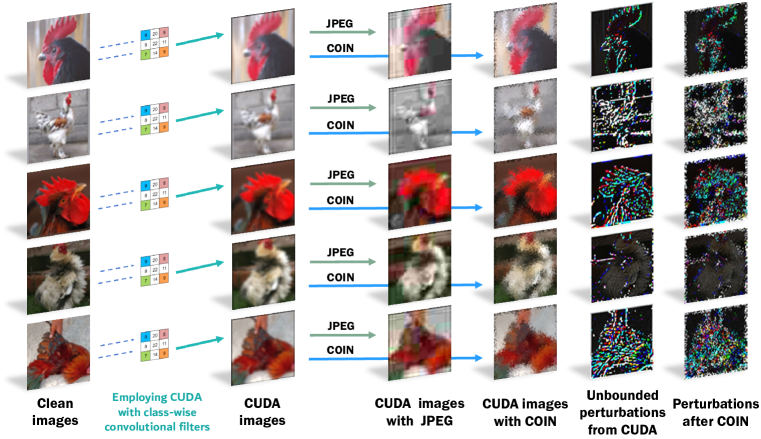
Figure 10: Clean images, CUDA images, CUDA images with JPEG defense and our defense COIN, and perturbations from class of ‘cock’ of the ImageNet UD.

A.5 Additional main experimental results and details

A.5.1 Additional main experiments on bounded UDs

While our COIN defense scheme is custom-designed for existing convolution-based UDs, we are also interested in its effectiveness against bounded UDs. We select four SOTA unlearnable techniques for generating bounded UDs (Fowl et al., 2021; Tao et al., 2021; Chen et al., 2023; Wu et al., 2023) and compare the results in test accuracy before and after using COIN, as shown in Table 11. Specific experimental parameter settings are completely consistent with the main experiments. The details of reproducing these three bounded UDs are given in Section A.5.2.

From the results in this table, we can see that COIN has effective defense capabilities against URP, TAP, and OPS. However, its defense effectiveness against SEP is limited and falls below an acceptable level. Therefore, while COIN greatly excels in defending against convolution-based UDs, it still has limitations when it comes to defending against bounded UDs.

A.5.2 Additional details

Standard data augmentations like random cropping and random flipping are adopted in our experiments. As for the generation process of convolution-based UDs, we also utilize their open-source code as follows:

• During generating CUDA UDs (Sadasivan et al., 2023), we directly run their official codes with default parameters https://github.com/vinusankars/Convolution-based-Unlearnability.

Remarks: Due to insufficient GPU capacity, a batch size of 64 was set when applying AA on CIFAR-10, CIFAR-100 using ResNet50.

During exploring COIN on bounded UDs, we mostly utilize their official codes. Detailed processes are as follows:

• For generating the TAP UD (Fowl et al., 2021), we simply crafted targeted adversarial exmples through PGD method (Madry et al., 2018) with iteration of 40, step size of 2/255 and perturbation budget of 8/255 in $\ell_{\infty}$-norm based on their unlearnable scheme.

• For generating the URP UD (Huang et al., 2021; Tao et al., 2021), we run the official codes https://github.com/TLMichael/Delusive-Adversary.

• For generating the SEP UD (Chen et al., 2023), we run their official codes https://github.com/Sizhe-Chen/SEP to produce UDs using ResNet18 checkpoints.

• During generating the OPS UD (Wu et al., 2023), we also run their official codes with default parametes https://github.com/cychomatica/One-Pixel-Shotcut.

A.6 Gaining a Visual Insight into Defense Methods

We visually demonstrate unlearnable images crafted by CUDA (CUDA images), along with their clean images and perturbations as shown in Fig. 10. We obtain “class-wise convolution-based perturbations from CUDA” by subtracting the corresponding clean images from the CUDA images. The perturbations from CUDA within the same class yet show non-identical noise, which differs to the class-wise form we understand in additive noise, and such noise does not exhibit linear separability like previous bounded UDs. To prove this, we train a linear logistic regression model on CUDA perturbations and report train accuracy following OP (Segura et al., 2023) and their official code, as shown in Table 10. This indicates that the added perturbations in CUDA are different from class-wise bounded perturbations, and indeed not totally linearly separable. Additionally, it can be observed that the JPEG transformation subjected to lossy compression tends to lose more features after employing CUDA images, which may be one of the reasons why JPEG compression fails to effectively defend against CUDA. After applying our COIN defense to CUDA images, visually, we are able to distinguish the specific categories of the images.

UDs	Train acc (%)	Is it linearly separable for added perturbations?
$\circ$EM (Huang et al., 2021)	100	YES
$\circ$Regions-4 (Sandoval-Segura et al., 2022a)	100	YES
$\circ$Random Noise	100	YES
CUDA (Sadasivan et al., 2023)	77.12	NO

Table 10: The linear separability of perturbations from UDs (“$\circ$” denotes class-wise noise patterns).

Bounded UDs$\rightarrow$	URP (Tao et al., 2021)			TAP (Fowl et al., 2021)			SEP (Chen et al., 2023)			OPS (Wu et al., 2023)
Defense$\downarrow$     Model$\rightarrow$	RN18	VGG19	AVG	RN18	VGG19	AVG	RN18	VGG19	AVG	RN18	VGG19	AVG
w/o	16.80	16.53	16.66	26.16	27.81	26.98	9.01	12.70	10.86	28.39	20.15	24.27
COIN	81.11	77.85	79.48	76.41	71.26	73.84	48.09	46.72	47.41	80.13	74.58	77.36

Table 11: The test accuracy results on three CIFAR-10 bounded UDs with and w/o applying COIN.

Input : Unbounded unlearnable dataset $\mathcal{D}_{u}=\{({x_{u}}_{i},y_{i})|i=1,2,\cdots,N,{x_{u}}_{i}\in\mathbb{R}^{C\times H\times W}\}$; range of random variables $\alpha$.

Output : Transformed dataset $\mathcal{D}_{t}=\{({x_{t}}_{i},y_{i})|i=1,2,\cdots,N,{x_{t}}_{i}\in\mathbb{R}^{C\times H\times W}\}$.

Function : Coordinate grid function meshgrid; uniform distribution $\mathcal{U}$; arange function returns evenly spaced values within a given interval; clip function clips values outside the interval to the interval edges.

1

2for $cnt=1$ to $N$ do

3       Sample random horizontal and vertical variables $s_{x},s_{y}\sim\mathcal{U}(-\alpha,\alpha,size=H\cdot W)$;

4      Initialize a coordinate grid $c_{x},c_{y}=meshgrid(arange(W),arange(H))$;

5      Initialize a pixel value list $L_{p}$ = [ ];

6      for $i=0$ to $H\cdot W-1$ do

7             Get a random horizontal and vertical location offset ${m_{x}}_{i}$ and ${m_{y}}_{i}$;

8            Calculate horizontal and vertical weight coefficient ${\omega_{x}}_{i}$ and ${\omega_{y}}_{i}$;

9            Obtain the coordinates of the nearest four points: ${q_{11}}_{i},{q_{21}}_{i},{q_{12}}_{i},{q_{22}}_{i}$;

10            for $j=1$ to $C$ do

11                   Apply bilinear interpolation to obtain new pixel value $\mathcal{F}_{j}(p_{i})$;

12                  $\mathcal{F}_{j}(p_{i})=clip(\mathcal{F}_{j}(p_{i}),0,1)$;

13             end for

14            

15            $L_{p}.append([\mathcal{F}_{1}(p_{i}),\mathcal{F}_{2}(p_{i}),\cdots,\mathcal{F}_{C}(p_{i})])$;

16       end for

17      

18      Output transformed image ${x_{t}}_{i}$ by filling the pixel values using $L_{p}$;

19 end for

Return: Transformed dataset $\mathcal{D}_{t}=\{({x_{t}}_{i},y_{i})|i=1,2,\cdots,N,{x_{t}}_{i}\in\mathbb{R}^{C\times H\times W}\}$.

Algorithm 2 Our defense COIN

References

- Blu et al. (2004) Thierry Blu, Philippe Thévenaz, and Michael Unser. Linear interpolation revitalized. IEEE Transactions on Image Processing, 13(5):710–719, 2004.
- Borgnia et al. (2021) Eitan Borgnia, Valeriia Cherepanova, Liam Fowl, Amin Ghiasi, Jonas Geiping, Micah Goldblum, Tom Goldstein, and Arjun Gupta. Strong data augmentation sanitizes poisoning and backdoor attacks without an accuracy tradeoff. In Proceedings of the 2021 IEEE International Conference on Acoustics, Speech and Signal Processing (ICASSP’21), pp. 3855–3859, 2021.
- Chen et al. (2023) Sizhe Chen, Geng Yuan, Xinwen Cheng, Yifan Gong, Minghai Qin, Yanzhi Wang, and Xiaolin Huang. Self-ensemble protection: Training checkpoints are good data protectors. In Proceedings of the 11th International Conference on Learning Representations (ICLR’23), 2023.
- Deng et al. (2009) Jia Deng, Wei Dong, Richard Socher, Li-Jia Li, Kai Li, and Li Fei-Fei. Imagenet: A large-scale hierarchical image database. In Proceedings of the 2009 IEEE/CVF Conference on Computer Vision and Pattern Recognition (CVPR’09), pp. 248–255, 2009.
- DeVries & Taylor (2017) Terrance DeVries and Graham W Taylor. Improved regularization of convolutional neural networks with cutout. arXiv preprint arXiv:1708.04552, 2017.
- Dolatabadi et al. (2023) Hadi M Dolatabadi, Sarah Erfani, and Christopher Leckie. The devil’s advocate: Shattering the illusion of unexploitable data using diffusion models. arXiv preprint arXiv:2303.08500, 2023.
- Fowl et al. (2021) Liam Fowl, Micah Goldblum, Ping-yeh Chiang, Jonas Geiping, Wojciech Czaja, and Tom Goldstein. Adversarial examples make strong poisons. In Proceedings of the 35th Neural Information Processing Systems (NeurIPS’21), volume 34, pp. 30339–30351, 2021.
- Friedman et al. (1997) Nir Friedman, Dan Geiger, and Moises Goldszmidt. Bayesian network classifiers. Machine Learning, 29:131–163, 1997.
- Fu et al. (2022) Shaopeng Fu, Fengxiang He, Yang Liu, Li Shen, and Dacheng Tao. Robust unlearnable examples: Protecting data privacy against adversarial learning. In Proceedings of the 10th International Conference on Learning Representations (ICLR’22), 2022.
- He et al. (2016) Kaiming He, Xiangyu Zhang, Shaoqing Ren, and Jian Sun. Deep residual learning for image recognition. In Proceedings of the 2016 IEEE/CVF Conference on Computer Vision and Pattern Recognition (CVPR’16), pp. 770–778, 2016.
- Hong et al. (2020) Sanghyun Hong, Varun Chandrasekaran, Yiğitcan Kaya, Tudor Dumitraş, and Nicolas Papernot. On the effectiveness of mitigating data poisoning attacks with gradient shaping. arXiv preprint arXiv:2002.11497, 2020.
- Hu et al. (2023) Shengshan Hu, Wei Liu, Minghui Li, Yechao Zhang, Xiaogeng Liu, Xianlong Wang, Leo Yu Zhang, and Junhui Hou. Pointcrt: Detecting backdoor in 3d point cloud via corruption robustness. In Proceedings of the 31st ACM International Conference on Multimedia (MM’23), pp. 666–675, 2023.
- Huang et al. (2017) Gao Huang, Zhuang Liu, Laurens Van Der Maaten, and Kilian Q Weinberger. Densely connected convolutional networks. In Proceedings of the 2017 IEEE/CVF Conference on Computer Vision and Pattern Recognition (CVPR’17), pp. 4700–4708, 2017.
- Huang et al. (2021) Hanxun Huang, Xingjun Ma, Sarah Monazam Erfani, James Bailey, and Yisen Wang. Unlearnable examples: Making personal data unexploitable. In Proceedings of the 9th International Conference on Learning Representations (ICLR’21), 2021.
- Javanmard & Soltanolkotabi (2022) Adel Javanmard and Mahdi Soltanolkotabi. Precise statistical analysis of classification accuracies for adversarial training. The Annals of Statistics, 50(4):2127–2156, 2022.
- Krizhevsky & Hinton (2009) Alex Krizhevsky and Geoffrey Hinton. Learning multiple layers of features from tiny images. 2009.
- Liu et al. (2023a) Xiaogeng Liu, Minghui Li, Haoyu Wang, Shengshan Hu, Dengpan Ye, Hai Jin, Libing Wu, and Chaowei Xiao. Detecting backdoors during the inference stage based on corruption robustness consistency. In Proceedings of the IEEE/CVF Conference on Computer Vision and Pattern Recognition (CVPR’23), pp. 16363–16372, 2023a.
- Liu et al. (2023b) Zhuoran Liu, Zhengyu Zhao, and Martha Larson. Image shortcut squeezing: Countering perturbative availability poisons with compression. In Proceedings of the 40th International Conference on Machine Learning (ICML’23), 2023b.
- Madry et al. (2018) Aleksander Madry, Aleksandar Makelov, Ludwig Schmidt, Dimitris Tsipras, and Adrian Vladu. Towards deep learning models resistant to adversarial attacks. In Proceedings of the 6th International Conference on Learning Representations (ICLR’18), 2018.
- Min et al. (2021) Yifei Min, Lin Chen, and Amin Karbasi. The curious case of adversarially robust models: More data can help, double descend, or hurt generalization. In Uncertainty in Artificial Intelligence, pp. 129–139. PMLR, 2021.
- Qin et al. (2023a) Tianrui Qin, Xitong Gao, Juanjuan Zhao, Kejiang Ye, and Cheng-Zhong Xu. Apbench: A unified benchmark for availability poisoning attacks and defenses. arXiv preprint arXiv:2308.03258, 2023a.
- Qin et al. (2023b) Tianrui Qin, Xitong Gao, Juanjuan Zhao, Kejiang Ye, and Cheng-Zhong Xu. Learning the unlearnable: Adversarial augmentations suppress unlearnable example attacks. arXiv preprint arXiv:2303.15127, 2023b.
- Ren et al. (2023) Jie Ren, Han Xu, Yuxuan Wan, Xingjun Ma, Lichao Sun, and Jiliang Tang. Transferable unlearnable examples. In Proceedings of the 11th International Conference on Learning Representations (ICLR’23), 2023.
- Reynolds et al. (2009) Douglas A Reynolds et al. Gaussian mixture models. Encyclopedia of Biometrics, 741(659-663), 2009.
- Sadasivan et al. (2023) Vinu Sankar Sadasivan, Mahdi Soltanolkotabi, and Soheil Feizi. Cuda: Convolution-based unlearnable datasets. In Proceedings of the 2023 IEEE/CVF Conference on Computer Vision and Pattern Recognition (CVPR’23), pp. 3862–3871, 2023.
- Sandler et al. (2018) Mark Sandler, Andrew Howard, Menglong Zhu, Andrey Zhmoginov, and Liang-Chieh Chen. Mobilenetv2: Inverted residuals and linear bottlenecks. In Proceedings of the 2018 IEEE Conference on Computer Vision and Pattern Recognition (CVPR’18), pp. 4510–4520, 2018.
- Sandoval-Segura et al. (2022a) Pedro Sandoval-Segura, Vasu Singla, Liam Fowl, Jonas Geiping, Micah Goldblum, David Jacobs, and Tom Goldstein. Poisons that are learned faster are more effective. In Proceedings of the 2022 IEEE/CVF Conference on Computer Vision and Pattern Recognition Workshops (CVPRW’22), pp. 198–205, 2022a.
- Sandoval-Segura et al. (2022b) Pedro Sandoval-Segura, Vasu Singla, Jonas Geiping, Micah Goldblum, Tom Goldstein, and David W Jacobs. Autoregressive perturbations for data poisoning. In Proceedings of the 36th Neural Information Processing Systems (NeurIPS’22), volume 35, 2022b.
- Segura et al. (2023) Pedro Sandoval Segura, Vasu Singla, Jonas Geiping, Micah Goldblum, and Tom Goldstein. What can we learn from unlearnable datasets? In Proceedings of the 37th Neural Information Processing Systems (NeurIPS’23), 2023.
- Simonyan & Zisserman (2014) Karen Simonyan and Andrew Zisserman. Very deep convolutional networks for large-scale image recognition. arXiv preprint arXiv:1409.1556, 2014.
- Szegedy et al. (2015) Christian Szegedy, Wei Liu, Yangqing Jia, Pierre Sermanet, Scott Reed, Dragomir Anguelov, Dumitru Erhan, Vincent Vanhoucke, and Andrew Rabinovich. Going deeper with convolutions. In Proceedings of the 2015 IEEE/CVF Conference on Computer Vision and Pattern Recognition (CVPR’15), pp. 1–9, 2015.
- Szegedy et al. (2016) Christian Szegedy, Vincent Vanhoucke, Sergey Ioffe, Jon Shlens, and Zbigniew Wojna. Rethinking the inception architecture for computer vision. In Proceedings of the 2016 IEEE/CVF Conference on Computer Vision and Pattern Recognition (CVPR’16), pp. 2818–2826, 2016.
- Tao et al. (2021) Lue Tao, Lei Feng, Jinfeng Yi, Sheng-Jun Huang, and Songcan Chen. Better safe than sorry: Preventing delusive adversaries with adversarial training. In Proceedings of the 35th Neural Information Processing Systems (NeurIPS’21), volume 34, pp. 16209–16225, 2021.
- Wen et al. (2023) Rui Wen, Zhengyu Zhao, Zhuoran Liu, Michael Backes, Tianhao Wang, and Yang Zhang. Is adversarial training really a silver bullet for mitigating data poisoning? In Proceedings of the 11th International Conference on Learning Representations (ICLR’23), 2023.
- Wu et al. (2023) Shutong Wu, Sizhe Chen, Cihang Xie, and Xiaolin Huang. One-pixel shortcut: On the learning preference of deep neural networks. In Proceedings of the 11th International Conference on Learning Representations (ICLR’23), 2023.
- Yu et al. (2022) Da Yu, Huishuai Zhang, Wei Chen, Jian Yin, and Tie-Yan Liu. Availability attacks create shortcuts. In Proceedings of the 28th ACM SIGKDD Conference on Knowledge Discovery and Data Mining (KDD’22), pp. 2367–2376, 2022.
- Yun et al. (2019) Sangdoo Yun, Dongyoon Han, Seong Joon Oh, Sanghyuk Chun, Junsuk Choe, and Youngjoon Yoo. Cutmix: Regularization strategy to train strong classifiers with localizable features. In Proceedings of the 17th International Conference on Computer Vision (ICCV’19), 2019.
- Zhang et al. (2018) Hongyi Zhang, Moustapha Cisse, Yann N. Dauphin, and David Lopez-Paz. Mixup: Beyond empirical risk minimization. In Proceedings of the 6th International Conference on Learning Representations (ICLR’18), 2018.
- Zhang et al. (2021) Longling Zhang, Bochen Shen, Ahmed Barnawi, Shan Xi, Neeraj Kumar, and Yi Wu. Feddpgan: Federated differentially private generative adversarial networks framework for the detection of covid-19 pneumonia. Information Systems Frontiers, 23(6):1403–1415, 2021.
- Zhou et al. (2023a) Ziqi Zhou, Shengshan Hu, Minghui Li, Hangtao Zhang, Yechao Zhang, and Hai Jin. Advclip: Downstream-agnostic adversarial examples in multimodal contrastive learning. In Proceedings of the 31st ACM International Conference on Multimedia (MM’23), pp. 6311–6320, 2023a.
- Zhou et al. (2023b) Ziqi Zhou, Shengshan Hu, Ruizhi Zhao, Qian Wang, Leo Yu Zhang, Junhui Hou, and Hai Jin. Downstream-agnostic adversarial examples. In Proceedings of the IEEE/CVF International Conference on Computer Vision (ICCV’23), pp. 4345–4355, 2023b.