Effective algorithms for calculation of quasiprobability distributions of bright “banana” states
Abstract
Non-Gaussian quantum states, described by negative valued Wigner functions, are important both for fundamental tests of quantum physics and for emerging quantum information technologies. One of the promising ways of generation of the non-Gaussian states is the use of the cubic (Kerr) optical non-linearity, which produces the characteristic banana-like shape of the resulting quantum states. However, the Kerr effect in highly transparent optical materials is weak. Therefore, big number of the photons in the optical mode () is necessary to generate an observable non-Gaussianity. In this case, the direct approach to calculation of the Wigner function becomes extremely computationally expensive.
In this work, we develop quick algorithms for computing the Husimi and Wigner quasiprobability functions of these non-Gaussin states by means of the Kerr nonlinearity. This algorithm can be used for any realistic values of the photons number and the non-linearity.
I Introduction
One of the priority tasks of quantum technologies is to design and build a universal quantum computer, allowing to provide an exponential speedup over classical computing. The promising approach to implementation of the quantum computing is based on the use of entangled modes of light (qumodes) and the corresponding continuous variables (quadrature amplitudes) of these modes [1, 2, 3]. The advantage of this approach is its very high degree of scalability [4]
The toolbox for the continuous variables quantum computing includes linear optical elements, such as beamsplitters and -nonlinearity based optical parametric amplifiers, described by the Hamiltonians which are quadratic in the quadrature amplitudes. An important feature of these elements is that they transform Gaussian quantum states (that is the ones described by the Guassian quasi-probability distributions, see Sec. II) again to Gaussian ones. At the same time, it is known that any setup which uses only Gaussian quantum states can be effectively simulated by the classical computer [5, 6]. Therefore, the key condition for achieving quantum supremacy is the use on non-linear elements and, correspondingly, non-Gaussian quantum states.
In the optical band, the most promising type of nonlinearity is the qubic (), or Kerr one (the higher order optical nonlinearities are negligibly small, see e.g. [7]). In the rotating wave picture, the Hamiltonian of optical mode with in such a nonlinearity is equal to [8]:
| (1) |
where is the nonlinearity parameter proportional to and inversely proportional to the mode volume [9, 10], and is the operator of the photons number in the mode. Since this Hamiltonian commutes with , the photon number distribution does not change during evolution. At the same time, the optical phase is modified proportionally (the self phase modulation effect, SPM). As a result, the quantum state of the optical mode acquires the characteristic non-Gaussian banana-like shape [9]. The degree on the non-Gaussianity is defined by the dimensionless parameter
| (2) |
where is the evolution time that should be much shorter than the intrinsic relaxation time of the mode . The values of
| (3) |
where is the mean photon number, correspond to the photon number uncertainties
| (4) |
that are unreachable by linear operations (squeezing). Therefore they can be considered as the “witness” of the non-Gaussianity [11, 9, 10].
Unfortunatetely, the Kerr effect in highly transparent optical materials is weak. This problem can be alleviated by concentration of the optical power in the small volume of the mode. The promising way to overcome this problem is the usage of optical ring resonators [12, 13], which combine the small volume of the mode with very high quality (more than in crystalline microresonators [14] and more than in on-chip ones [15, 16]). However, even in the best modern microresonators,
| (5) |
see e.g. esimates in Ref. [10], which translates to the values
| (6) |
For the theoretical study of the “banana” states, it is necessary to calculate their quasi-probability distributions, namely the Husimi and Wigner functions (see Sec. II). However, here the computational problem arises. While the Husimi function can be calculated directly using its definition without significant difficulties [17], calculation of the Wigner function is much more involved.
Two methods of numerical calculation of the Wigner function were typically used in literature: by solving the differential equation on its evolution over time, or directly by calculating it for each point. As the results of Ref. [18] show, the known formulas for direct calculation turn out to be inapplicable for large . In addition to causing overflows quickly, they also require about summands, which makes them very computationally expensive.
In this paper, we build an alternative approach to the computation of the Husimi and Wigner functions based on asymptotic estimates that utilize the smallness of and the large value of . The paper is organized as follows. In Sec. II, we briefly overview the main features of the Husimi and Wigner functions. Then, in Sections III and IV, we develop the fast algorithms for numerical computing of the Husimi and Wigner function, respectively. In Sec. V, we summarize the main results of this paper.
II Introduction to Husimi and Wigner functions
The quantum quasi-probability distributions [19, 20, 21, 22] serve as conveninent substitutes for the joint probability distributions for the positions and momenta of quantum objects. They have one-to-one correspondence with the respective quantum states and can be experimentally reconstructed using the quantum tomography procedure [23].
It is convenient to introduce the quantum quasi-probability distributions, using the s-parametrized characteristic function, defined as follows [22]:
| (7) |
where , are the annihilation and creation operator, is the density operator, is a complex number, and is a real parameter with . The Wigner function [19] is equal to the inverse Fourier transform of the symmetrical ordered () characteristic function
| (8) |
where
| (9) |
and , are the normalized position and momentum. The distinctive feature of the Wigner functaion is that in the Gaussian case, it is exactly equal to the corresponding classical probability distribution. However, the Wigner functions of all other (non-Gaussian) pure quantum states take negative values [24]. It is this feature actually makes the these states “truly quantum”. The Wigner function can be measured indirectly using homodyne detection, which makes the experimental verification of these results relatively simple [25].
The inverse Fourier transform of the anti-normal ordered () characteristic function gives the Husimi -function [20]:
| (10) |
where is a coherent state. It is non-negative everywhere and can be obtained from the Wigner function by the Gaussian blurring operation.
Yet another quasi-probability distribution, the Glauber -function [21], correspond to the normal ordering case of . However, it is highly singular for all pure quantum states except of the ground and coherent ones. Therefore, we will not consider it here.
III Calculation of Husimi function
Evolution of the initial coherent quantum state with the Hamiltonian (1) during the time gives the following wave function:
| (11) |
Using then the definition (10), we obtain the following equation for the corresponding Husimi function:
| (12) |
Note that and appear in the Husimi function series only in combination . Therefore, let us introduce the function
| (13) |
Using this notation, the Husimi function (12) can be expressed as follows::
| (14) |
The nonlinear evolution factor in Eq. (13) can be presented as follows:
| (15) |
where stands for the Cauchy principal value integral. Therefore,
| (16) |
where
| (17a) | |||
| (17b) | |||
The integral in Eq. (16) can be calculated using the saddle point method [26]. In our case, the number of pass points is infinite (). They can be numbered according to the numbers of branches of the Lambert -function:
| (18) |
The schematic positions of the saddle points and the constant phase lines passing through them is shown in Fig. 1. Note that there are two constant phase lines for each of : one of them corresponds to the line of steepest descent at , and the other — at .
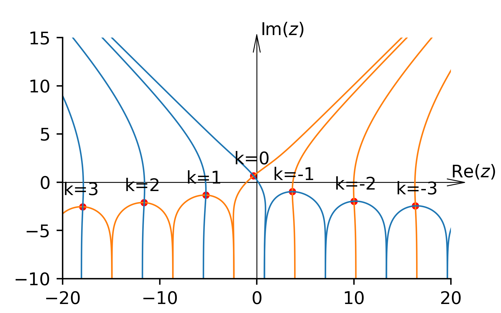
A detailed analysis at how to deform the integration contour and account for residual terms using the Campbell–Froman–Walles–Wojdylo (CFWW) formula [27] is done in Appendix A. It is shown there that the deformed contour passes through only half of all , which gives to the following result:
| (19) |
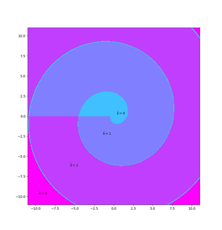
This equation is still not convenient for numerical calculations, because it contains an infinite sum. However, due to the smallness of , the term , as a function of , has a very narrow Gaussian profile. It is shown in Appendix B, that due to this reason, that out of the whole sum in the equation (19), only one or two summands should be kept, as shown, in Figure 2, and in most cases, it is sufficient to keep only one summand with the number
| (20) |
where means rounding to the nearest integer. As a result, we obtain the following closed equation for the Husimi function:
| (21) |
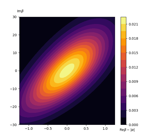
A characteristic example of the Husimi function, calculated using this equation, is shown in Fig. 3.
IV Wigner function
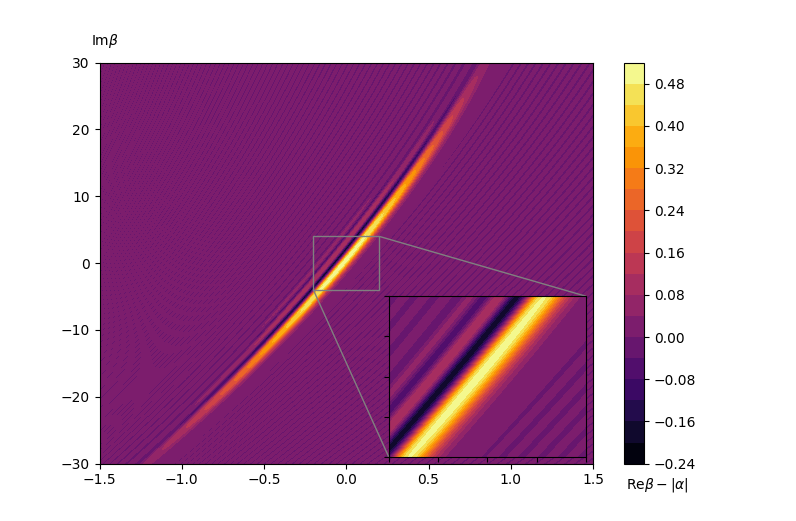
The basic idea for finding the values of the Wigner function is to relate it to the Husimi function using Eqs. (7), (8), and (10):.
| (22) |
However, for the numerical calculation, we cannot use directly in this equation the already obtained approximation for the Husimi function (21) due to the exponential factor . At the same time, if is a rational number:
| (23) |
where , are integers, then the following closed expression with a finite number of summands exists for the function :
| (24) |
see Appendix C. Any particular gamma observed in an experiment will almost surely be irrational. However, since the rational numbers are dense in the set of real numbers, this formula can approximate the actual dependence as accurately as necessary with a proper choice of and .
The representation (24) together with (14) is very convenient, since it reduces calculation the Fourier transforms (22) to computation of Gaussian integrals, see Appendix D. The result is the following formula, which is valid for arbitrary :
| (25) |
This form is still can not be used directly in numerical calculations. In the most meaningful case it may be shown that as well as for the coherent state for some . The maximum of have the order of magnitude of . Therefore, to get values we need to sum numbers of order with the accuracy of order , which is unattainable at large .
In order to evade this problem, let us decompose the expression (25) into a Fourier series in :
| (26) |
Here we can use the asymptotics for the modified Bessel function , which are valid both for small and large values . Using Eq. (79) and assuming that , we obtain the following equation for the Wigner function:
| (27) |
where is determined numerically based on the required accuracy.
V Conclusion
The fast algorithms developed in this work allow to radically accelerate calculation of quasi-probability distribution of the the mutli-photon “banana” states.
The standard algorithm for computing the Husimi function, based on the direct computation of the sum of Poisson distributed terms (12), require the computing time that scales as . The algorithm which we developed here, allows one to calculate the Husimi function for operations.
In the case of the Wigner function, the difference is much more significant. The direct algorithm requires operations and leads to overflow when is large. Our algorithm requires the computing time that scales as only.
The software implementation of these algorithms is available on the github [28].
Acknowledgements.
I appreciate assistance and guidance from Farit Khalili. This work was supported by the Russian Science Foundation (project 20-12-00344).Appendix A Series for Husimi functions
A.1 Contour deformation
The purpose of this section is to show how the integration contour on the complex plane can be deformed using the following function:
| (28) | ||||
We will consistently apply the steepest descent method.
A.1.1 Pass points
First we find the pass points satisfying the equation :
| (29) |
where is the -function of the Lambert function. Note that it has an infinite number of branches numbered by integer . Let’s index the pass points according to this numbering:
| (30) |
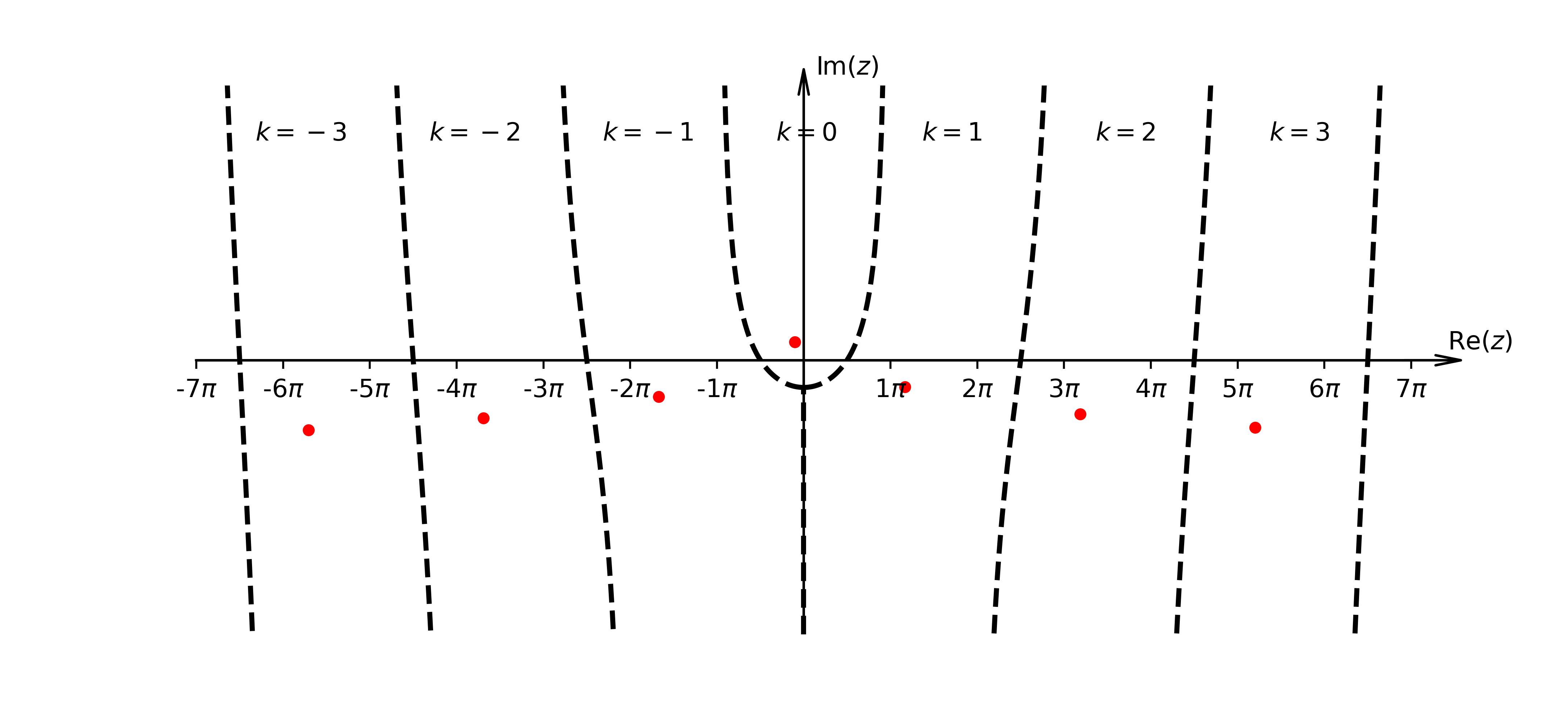
Figure 5 illustrates the possible locations of . A special case that we will not consider is . By excluding this special , we can say that all are distinct from each other, are second-order pass points () and every one of them satisfies .
A.1.2 Asymptotics of constant phase curves
Let us consider some point . Since and , there are two constant phase curves through . One of these is the steepest descent curve and the other is the steepest growth curve. (These curves change when the sign of changes.) Let us assume a natural parameterization of the fastest descent curve :
| (31) |
Based on the asymptotic behavior of the constant phase curve, we can obtain two cases of the last expression:
| (32) |
Combined with the previous paragraph, this reasoning confirms that the constant phase curves in Figure 1 have a general pattern that holds for any .
A.1.3 Final contour
The Fig. 6 shows the proposed in (LABEL:main_integral) integration contours for the case . (For , however, runs through nonnegative instead of nonpositive indices, resulting in a symmetric picture.) The expression (LABEL:main_integral) is a principal value integral, so we can integrate from to , then take . Figure 6 shows how we deform the contour. In order to leave only the integrals along the constant phase curves, we prove that the integrals and along the vertical lines tend to .
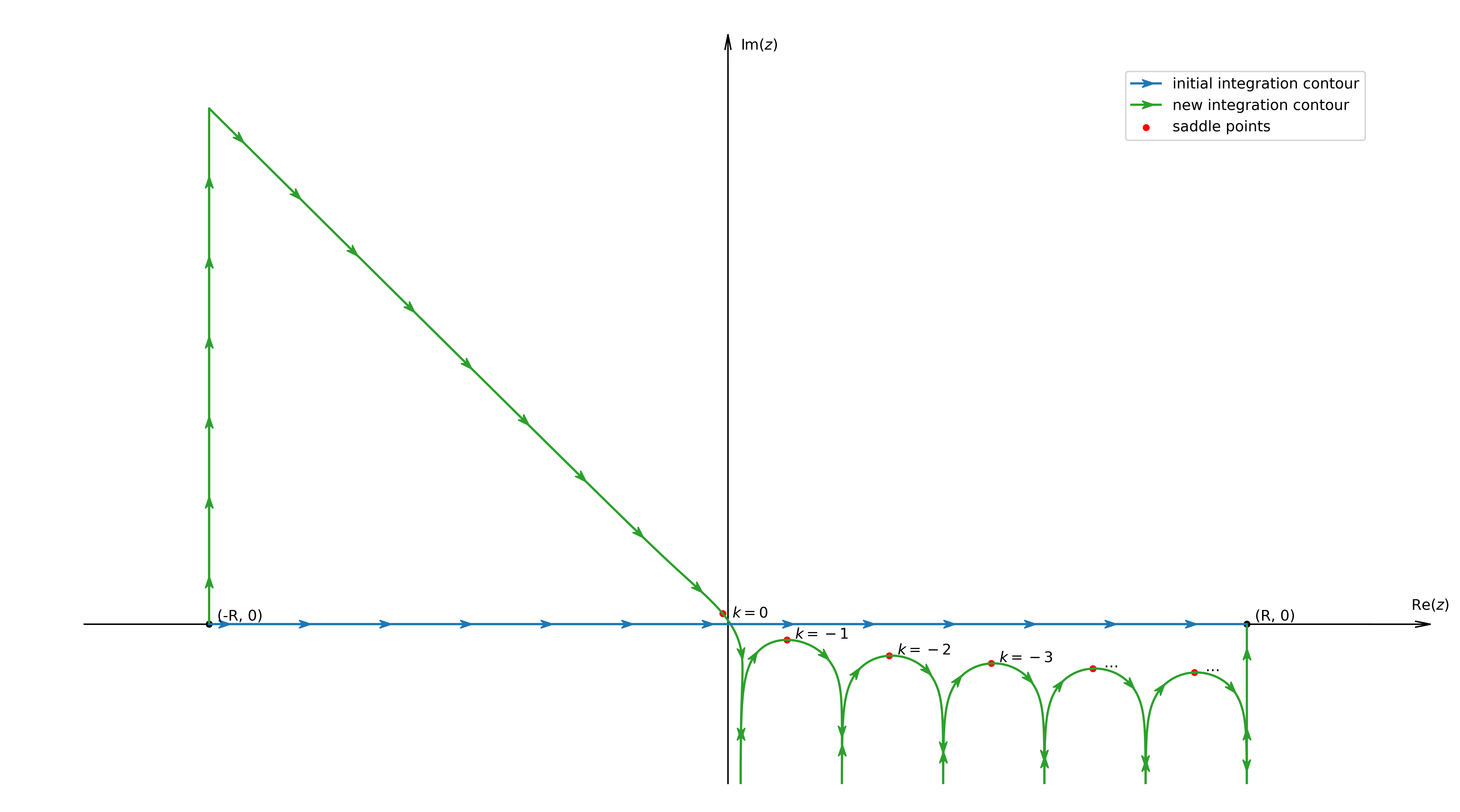
| (33) | ||||
We draw the vertical line for the calculation of at the abscissa such that . It is easy to see that such are dense in the neighborhood of the point , which is enough to neglect when computing the principal value integral.
| (34) | ||||
This gives us the formula useful for further calculations:
| (35) |
A.2 Residual terms by CFWW formula
A.2.1 Application of CFWW
To calculate the integral along some , we will use the CFWW [27] formula. Using this method, we need a Taylor series expansion of the function around the pass point:
| (36) |
To use CFWW, we mentally divide the integration contour into two parts starting at and going to infinity. Taking into account that the pass point has the second order, let us write down the final result:
| (37) | ||||
where are the partial (exponential) Bell polynomials of the coefficients in the Taylor series expansion of (36).
Bell’s partial polynomials are given by the following generating function:
| (38) |
It is easy to deduce from this definition:
| (39) |
In our case, and , so we only need to compute Bell polynomials of the form . These polynomials can be reduced to the well-studied associated Stirling numbers at , which are discussed in more detail in the next subsection.
A.2.2 Bell polynomials and associated Stirling numbers
In this subsection we will prove the following formula:
| (40) |
The right-hand side of the equation is more computationally convenient because can be read by the recurrence formula[29, p. 222]
| (41) |
The proof of the (40) follows directly from a comparison of the derivative functions of Bell polynomials (38) and the associated Stirling numbers [29, p. 222]:
| (42) |
| (43) | ||||
A.2.3 The final expression for the sum
First we put together the formulas (36), (37), (39), and (40).
| (44) | ||||
Finally, we can substitute this into (37), (35), and (LABEL:main_integral) to get an expression for the sum:
| (45) | ||||
We would like to mention the choice of the root branch. Since the original integral (LABEL:main_integral) was taken within , also has a left-to-right direction, which leads to:
| (46) |
Appendix B Contributions from different branches of the Lambert function
B.1 Dependence on
In this section we consider the expression (45) in approximate form:
| (47) |
Such an expression is still not convenient for computer calculations, because it contains an infinite sum. In this case, a natural question arises: which terms make the main contribution to the sum (45)? Due to the smallness of , the most important parameter for comparing the absolute values of the summands is as a function of . When is relatively small (recall that ), this question is easily solved numerically, which is given by 2. However, for large , we can use the decomposition for the Lambert -function [30, formula 4.20] and give the following expression:
| (48) |
It clearly shows an expression for , which is the major contributor to the sum (45):
| (49) |
where means rounding to the nearest integer. The decomposition of (48) shows that we can often restrict ourselves to just one summand of the whole sum:
| (50) |
where is defined as follows:
| (51) |
indicates how inaccurately was rounded.
B.2 Contribution decomposition by
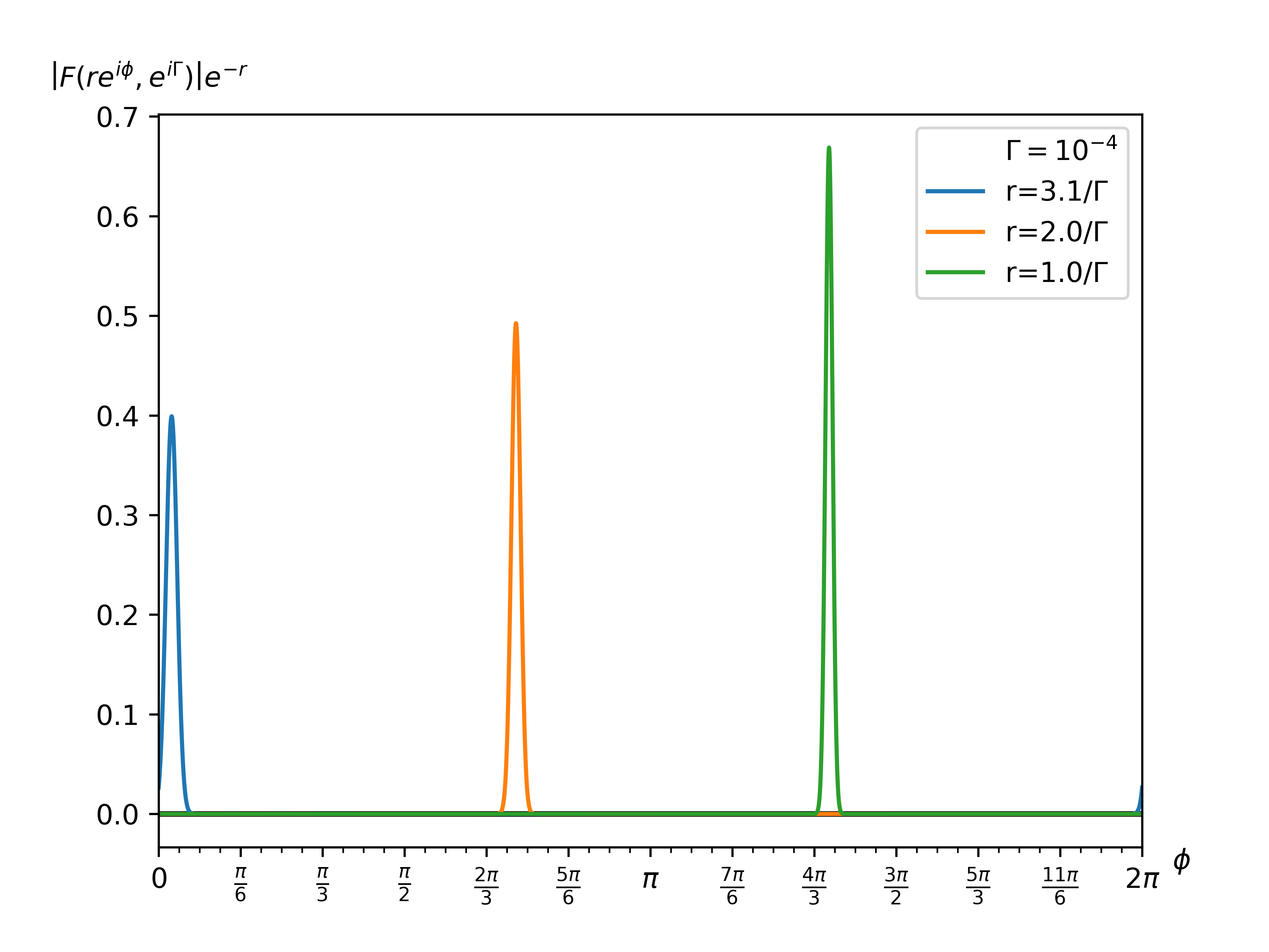
For large , one can notice that the series (LABEL:main_integral) as a function of has a very narrow profile 7. As follows from (50), the main contribution is a multiplier of the form . Explicitly expressing through the Lambert function,
| (52) |
and using [30, formula 3.2] we can find where the peak value is reached:
| (53) |
Next, from the definition of Lambert’s -function:
| (54) |
The uncertainty in the sign of can be removed by considering that we are looking for a maximum, not an arbitrary extremum:
| (55) |
Using the definition of the Lambert -function, we find :
| (56) |
By taking higher order derivatives of [30, formula 3.5], the behavior in the neighborhood of the maximum point can be obtained:
| (57) | ||||
where the notation — Euler numbers of the second kind.
Appendix C An alternative form of writing
Recall the definition of the function given in the article:
| (58) |
In the case , where is an irreducible fraction with odd denominator, we can see that the multiplier runs over a finite set of values. This allows us to decompose the sum (58) into sums, each of which is part of a Taylor series for the exponent. In the current section, however, we consider the approach via a functional-differential equation. In order to simplify the expressions, we assume .
| (59) |
This equation relates the derivative at point to the value at point , which is on the complex plane on a circle of the same radius . Taking again the derivatives at the point , we obtain:
| (60) | ||||
This is how we obtained the ordinary linear differential equation. To solve it, we need to choose different roots of . Since we have chosen such that and are coprime, the different degrees of completely span the entire set of :
| (61) |
The equation on the constants can be found by comparing the partial derivatives of the latter expression with (59):
| (62) | ||||
The constant can be found from the value , which leads to the following expression:
| (63) |
Appendix D Derivation of the relationship between the Wigner and Husimi functions
In the main body of the article, it was mentioned that the Husimi function is related to the function as follows:
| (64) |
We use the notation and from the previous section:
| (65) | ||||
In this section, we use the following well-known relation between Husimi and Wigner functions via characteristic functions:
| (66) |
Let us sequentially compute the contribution from each to . The following calculations are planned as follows:
| (67) | ||||
For these calculations we need formulas, the verification of which is done by taking Gaussian integrals:
| (68) | ||||
So, let us start with the contribution of to the antisymmetric characteristic function part :
| (69) | ||||
then continue with its contribution to the Wigner function:
| (70) | ||||
and finally, sum all the resulting contributions:
| (71) | ||||
The resulting expression is very well summarized through the previously introduced . Let us eliminate the derivatives by reasoning similar to the derivation of the functional-differential equation (59):
| (72) | ||||
| (73) |
Finally, let us reduce the expression to a form containing only the Husimi and Wigner functions:
| (74) |
It is important to note that this result is continuous on on the unit circle, and can be applied to any real .
Appendix E Wigner function series
E.1 Fourier series for the function
According to the article, decomposing the Wigner function into a Fourier series is the fastest and most accurate method of calculating it.
| (75) | ||||
Let us further substitute . In such notations .
| (76) | ||||
Second line summation is based on modified Bessel function . By substituting this into the formula above, we get:
| (77) |
Using the notation and substituting (77) into (73), we obtain:
| (78) | ||||
E.2 The required number of summands
E.2.1 Division into areas of
The equation (78) is still inconvenient for direct computations on a computer. Let us write out the asymptotic expression [31, p. 86] for the modified Bessel function through the auxiliary :
| (79) | ||||
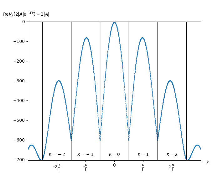
Note that has a rather smooth dependence on and a very strong dependence on . reaches local maxima when is in the neighborhood of the real axis. This is important because in the sum (78) both the parameter and the phase of the argument change simultaneously. When is small, it is convenient to divide the regions numbered with by the number of times occurs near the real axis. As can be seen from the graph 8, the contribution from the region is the largest. The contributions of the other regions will be evaluated in the next subsection.
E.2.2 Contributions from
To neglect contributions from regions with , the accuracy of this approximation must be determined. The function as a function of is decreasing, and hence to evaluate the accuracy it is sufficient to compare the contributions from and . Here we give the reasoning for and (for other the reasoning is similar, but rather cumbersome):
| (80) |
We temporarily introduce the variable and show the difference in peak contributions:
| (81) |
The function from marked by the bracket is everywhere less than zero at . Thus, the magnitude of the summands at is exponentially suppressed.
E.2.3 Contributions from
In the neighborhood of , the function has a single maximum at . Let us write the expression for the Wigner function:
| (82) |
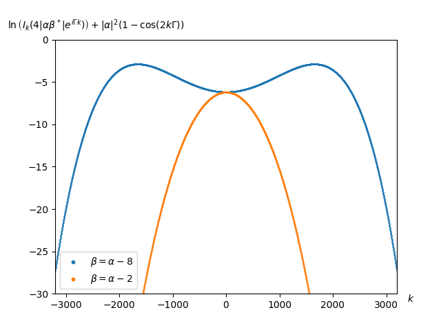
In the sum (82) it can be seen that the modules of the terms coincide when replacing . When the function is strictly decreasing. The addition of can lead to splitting the maximum into two, as shown in Figure 9. The condition for such splitting is the growth of the modules of the terms at . Considering as a continuous variable, we can find for changing the sign of the second derivative at :
| (83) |
Counting , this expression can be simplified:
| (84) |
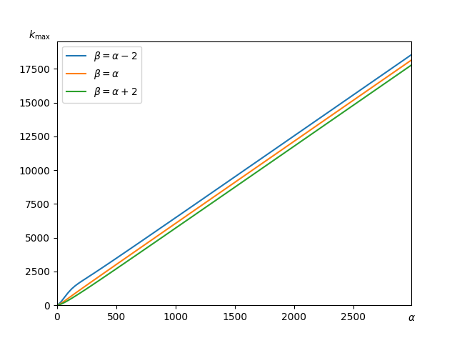
Thus, at , maximum splitting does not occur, which means that the summands in the sum of (82) will monotonically decrease at any . With and , the terms will behave nonmonotonically with increasing . Since , we can assume that in the most meaningful area, where , figure 9 is almost incredible in calculations. Nevertheless, the dependence of the modules of the summands is too complex to write out the upper limit of the sum (27) necessary to obtain a given accuracy. In the software implementation, you can use a simple binary search to find the required . Numerical calculations show that 10.
References
- Lloyd and Braunstein [1999] S. Lloyd and S. L. Braunstein, Quantum computation over continuous variables, Phys. Rev. Lett. 82, 1784 (1999).
- Braunstein and van Loock [2005] S. L. Braunstein and P. van Loock, Quantum information with continuous variables, Rev. Mod. Phys. 77, 513 (2005).
- Weedbrook et al. [2012] C. Weedbrook, S. Pirandola, R. García-Patrón, N. J. Cerf, T. C. Ralph, J. H. Shapiro, and S. Lloyd, Gaussian quantum information, Rev. Mod. Phys. 84, 621 (2012).
- Pfister [2019] O. Pfister, Continuous-variable quantum computing in the quantum optical frequency comb, Journal of Physics B: Atomic, Molecular and Optical Physics 53, 012001 (2019).
- Bartlett et al. [2002] S. D. Bartlett, B. C. Sanders, S. L. Braunstein, and K. Nemoto, Efficient classical simulation of continuous variable quantum information processes, Phys. Rev. Lett. 88, 097904 (2002).
- Mari and Eisert [2012] A. Mari and J. Eisert, Positive wigner functions render classical simulation of quantum computation efficient, Phys. Rev. Lett. 109, 230503 (2012).
- Ekvall et al. [2001] K. Ekvall, C. Lundevall, and P. van der Meulen, Studies of the fifth-order nonlinear susceptibility of ultraviolet-grade fused silica, Optics Letters 26, 896 (2001).
- Leonard Mandel [1984] E. W. Leonard Mandel, Coherence and Quantum Optics V: Proceedings of the Fifth Rochester Conference on Coherence and Quantum Optics held at the University of Rochester, June 13–15, 1983, 1st ed. (Springer, 1984) p. 751.
- Kitagawa and Yamamoto [1986] M. Kitagawa and Y. Yamamoto, Number-phase minimum-uncertainty state with reduced number uncertainty in a kerr nonlinear interferometer, Phys. Rev. A 34, 3974 (1986).
- Balybin et al. [2020] S. N. Balybin, F. Y. Khalili, D. V. Strekalov, A. B. Matsko, and I. A. Bilenko, On perspectives of generating quasi-Fock state via resonant self-phase-modulation, in Quantum and Nonlinear Optics VII, Vol. 11558, edited by K. Shi, D.-S. Kim, and C.-F. Li, International Society for Optics and Photonics (SPIE, 2020) pp. 9 – 24.
- Bondurant and Shapiro [1984] R. S. Bondurant and J. H. Shapiro, Squeezed states in phase-sensing interferometers, Phys. Rev. D 30, 2548 (1984).
- V.B.Braginsky, M.L.Gorodetsky, V.S.Ilchenko [1989] V.B.Braginsky, M.L.Gorodetsky, V.S.Ilchenko, Quality-factor and nonlinear properties of optical whispering-gallery modes, Physics Letters A 137, 393 (1989).
- Strekalov et al. [2016] D. V. Strekalov, C. Marquardt, A. B. Matsko, H. G. L. Schwefel, and G. Leuchs, Nonlinear and quantum optics with whispering gallery resonators, Journal of Optics 18, 123002 (2016).
- Savchenkov et al. [2007] A. A. Savchenkov, A. B. Matsko, V. S. Ilchenko, and L. Maleki, Optical resonators with ten million finesse, Opt. Express 15, 6768 (2007).
- Kippenberg et al. [2004] T. J. Kippenberg, S. M. Spillane, and K. J. Vahala, Kerr-nonlinearity optical parametric oscillation in an ultrahigh- toroid microcavity, Phys. Rev. Lett. 93, 083904 (2004).
- Wu et al. [2020] L. Wu, H. Wang, Q. Yang, Q. xin Ji, B. Shen, C. Bao, M. Gao, and K. Vahala, Greater than one billion q factor for on-chip microresonators, Opt. Lett. 45, 5129 (2020).
- Rosiek [2022] C. A. Rosiek, Enhancing the formation of wigner negativity in a kerr oscillator via quadrature squeezing, arXiv preprint arXiv:2202.02285 , 61 (2022).
- Stobińska et al. [2008] M. Stobińska, G. Milburn, and K. Wódkiewicz, Wigner function evolution of quantum states in the presence of self-kerr interaction, Physical Review A 78, 013810 (2008).
- Wigner [1932] E. Wigner, On the quantum correction for thermodynamic equilibrium, Phys. Rev. 40, 749 (1932).
- Husimi [1940] K. Husimi, Some formal properties of the density matrix, Proceedings of the Physico-Mathematical Society of Japan. 3rd Series 22, 264 (1940).
- Glauber [1963] R. J. Glauber, Coherent and incoherent states of the radiation field, Phys. Rev. 131, 2766 (1963).
- Cahill and Glauber [1969] K. E. Cahill and R. J. Glauber, Density operators and quasiprobability distributions, Phys. Rev. 177, 1882 (1969).
- Vogel and Risken [1989] K. Vogel and H. Risken, Determination of quasiprobability distributions in terms of probability distributions for the rotated quadrature phase, Phys. Rev. A 40, 2847 (1989).
- Hudson [1974] R. Hudson, When is the wigner quasi-probability density non-negative?, Reports on Mathematical Physics 6, 249 (1974).
- W. Schleich [2001] W. Schleich, Quantum Optics in Phase Space (WILEY-VCH, Berlin, 2001) p. 695.
- Fedoryuk [1977] M. Fedoryuk, The saddle-point method (1977).
- Bleistein and Handelsman [1975] N. Bleistein and R. A. Handelsman, Asymptotic expansions of integrals (Ardent Media, 1975).
- [28] https://github.com/KeeeeeK/SPM-distributions.
- Comtet [2012] L. Comtet, Advanced Combinatorics: The art of finite and infinite expansions (Springer Science & Business Media, 2012).
- Corless et al. [1996] R. M. Corless, G. H. Gonnet, D. E. Hare, D. J. Jeffrey, and D. E. Knuth, On the lambertw function, Advances in Computational mathematics 5, 329 (1996).
- Bateman [1953] H. Bateman, Higher transcendental functions, Vol. 2 (McGRAW-HILL book company, 1953).