Prompt-Based Exemplar Super-Compression and Regeneration
for Class-Incremental Learning

Abstract

Replay-based methods in class-incremental learning (CIL) have attained remarkable success, as replaying the exemplars of old classes can significantly mitigate catastrophic forgetting. Despite their effectiveness, the inherent memory restrictions of CIL result in saving a limited number of exemplars with poor diversity, leading to data imbalance and overfitting issues. In this paper, we introduce a novel exemplar super-compression and regeneration method, ESCORT, which substantially increases the quantity and enhances the diversity of exemplars. Rather than storing past images, we compress images into visual and textual prompts, e.g., edge maps and class tags, and save the prompts instead, reducing the memory usage of each exemplar to $\frac{1}{24}$ of the original size. In subsequent learning phases, diverse high-resolution exemplars are generated from the prompts by a pre-trained diffusion model, e.g., ControlNet [50]. To minimize the domain gap between generated exemplars and real images, we propose partial compression and diffusion-based data augmentation, allowing us to utilize an off-the-shelf diffusion model without fine-tuning it on the target dataset. Therefore, the same diffusion model can be downloaded whenever it is needed, incurring no memory consumption. Comprehensive experiments demonstrate that our method significantly improves model performance across multiple CIL benchmarks, e.g., $5.0$ percentage points higher than the previous state-of-the-art on $10$-phase Caltech-256 dataset.

1 Introduction

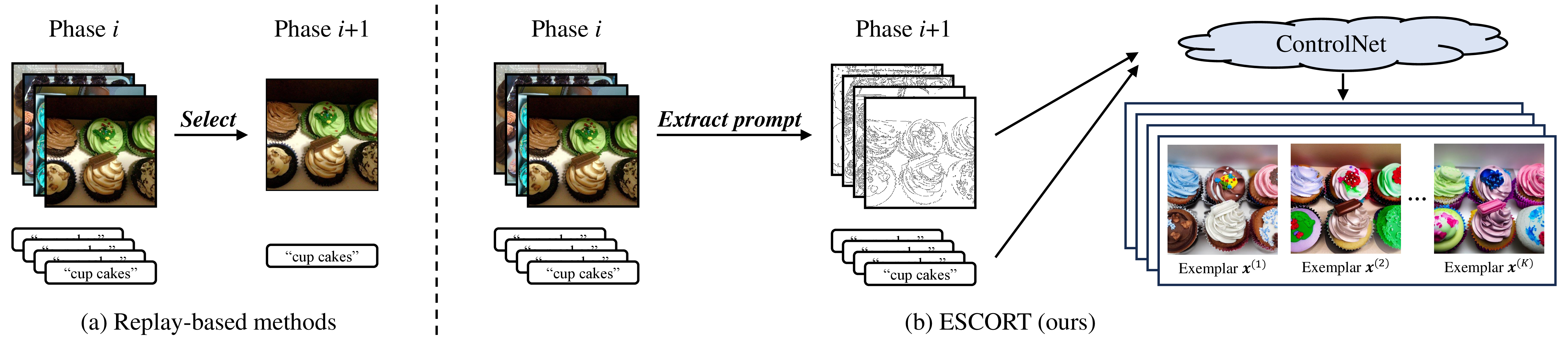
Figure 1: Comparison between traditional replay-based CIL methods with our approach. (a) Traditional replay-based CIL methods can only select and save a small number of exemplars due to memory constraint, leading to two severe problems: firstly, the relative small size of the exemplar set compared to the new training data gives rise to a pronounced imbalance between old and new classes; secondly, the limited diversity of the exemplar set compared to the original training set incurs overfitting problem. (b) ESCORT compresses the old images into visual and text prompts, e.g., edge maps and class tags, and saves these prompts to the memory. In subsequent phases, diverse high-resolution exemplars are generated from these prompts via an off-the-shelf pre-trained diffusion model, e.g., ControlNet [50]. With ESCORT, the data imbalance and overfitting problems are significantly alleviated.

Ideally, AI systems should be adaptive to ever-changing environments—where the data are continuously observed. The AI models should be capable of learning concepts from new data while maintaining the ability to recognize the old ones. In practice, AI systems often have constrained memory budgets, because of which most of the historical data must be abandoned. However, deep AI models suffer from catastrophic forgetting when continuously updated using new data and limited historical data, as previous knowledge can be overridden by the new information [34, 38]. To study how to overcome catastrophic forgetting, the class-incremental learning (CIL) protocol [39] was established. CIL assumes training samples from various classes are introduced to the model in phases, with previous data largely discarded from memory.

CIL has experienced significant advancements over the years [22, 49, 2, 7, 23, 48, 47, 45, 54, 36, 51, 30, 29]. Among these, replay-based methods [39, 18, 26, 27, 47, 25] stand out in terms of performance by employing a memory buffer to store a limited number of representative samples (i.e., exemplars) from former classes. During subsequent learning phases, these exemplars are revisited to help retain previously learned knowledge. Although replay-based methods demonstrate notable effectiveness, they encounter two main issues. Firstly, the exemplar set is much smaller compared to new training data, resulting in a significant imbalance between the new and old classes. Secondly, the poor diversity of the exemplar set compared to the original training set can induce overfitting.

In this paper, we address these issues by proposing a novel method named Exemplar Super-COmpression and Regeneration based on prompTs (ESCORT). Instead of directly storing the previous images, we compress them into visual and textual prompts, e.g., edge maps and class tags, and save these prompts in the memory. In subsequent phases, diverse high-resolution exemplars are regenerated from the prompts by leveraging an off-the-shelf pre-trained diffusion model, e.g., ControlNet [50].

Compared to traditional direct replay methods, ESCORT enjoys increased quantity and enhanced diversity of the exemplar set, as illustrated in Fig. 1. Firstly, the exemplar quantity is boosted by compression: since the memory consumption of a $1$-bit edge map is merely $\frac{1}{24}$ that of its $8$-bit, $3$-channel RGB image counterpart, $24$ times more exemplars can be saved within the same memory consumption. We call this process super-compression as this compression ratio is far beyond that of existing image compression algorithms without any reduction of image quality. Secondly, instead of relying on the images only from the dataset itself, diffusion-based image generation produces unseen samples with great diversity, which can be obtained simply by changing the random seed of the diffusion model.

However, utilizing generated images for CIL model training leads to a potentially huge domain gap between old exemplars and new data. We propose two techniques to tackle this problem, i.e., partial compression and diffusion-based data augmentation, enabling the CIL model to properly benefit from the synthetic exemplars without the need to fine-tune the diffusion model on the target dataset. Partial compression employs a small proportion of the memory to store prompts for exemplar regeneration and the rest to store real images. In later phases, the model is trained by a mixed set of recreated exemplars and real-image exemplars. Diffusion-based data augmentation involves the usage of an off-the-shelf diffusion model to generate data during CIL training, when each real image is sometimes replaced by its synthetic counterpart. Since the same pre-trained diffusion model can be directly downloaded from the public cloud at any time when necessary, we do not need to store the fine-tuned generator using our own memory.

Extensive experiments are conducted on three image classification datasets: Caltech-256 [13], Food-101 [5], and Places-100 [53]. We fully investigate the effect of ESCORT under different CIL settings and demonstrate that our approach achieves substantial improvements compared to the state-of-the-art CIL method, e.g., increasing average accuracy on Caltech-256 by $5.0$ percentage points.

To summarize, we make three contributions: 1) a novel exemplar compression and regeneration method for CIL to increase the quantity and enhance the diversity of exemplars, 2) two techniques, i.e., partial compression and diffusion-based data augmentation, to alleviate the domain gap between generated and real exemplars, and 3) extensive experiments on three CIL datasets with state-of-the-art results, an in-depth ablation study, and further visualizations.

2 Related Work

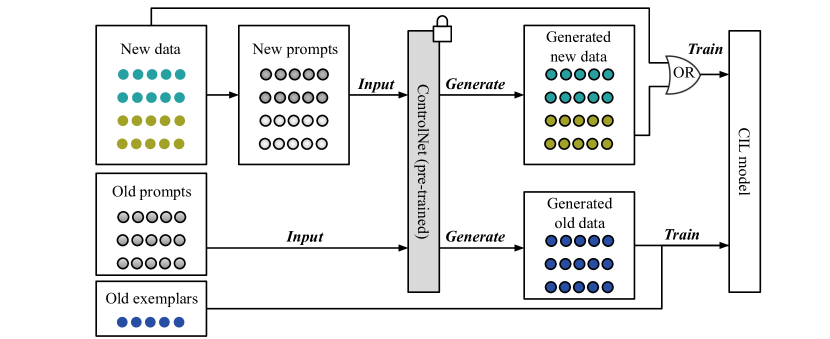
Figure 2: The CIL model training process with ESCORT in the $i$-th phase ($i\geq 2$). A pre-trained ControlNet is downloaded in advance and remains frozen during this stage for image generation. Initially, we have three subsets of data because of partial compression: new images of this phase, old prompts (i.e., edge maps and class tags), and old real-image exemplars. For the old data, we transform the prompts to synthetic images by ControlNet and use both generated and real images of old classes for model training. For the new images, we transform them into prompts as well and obtain their generated version. Data augmentation is performed by randomly replacing some real new images with their synthetic copies in every epoch during training.

Class-incremental learning The goal of class-incremental learning is to develop machine learning models that can effectively adapt and learn from data presented in a series of training stages. This is closely associated with topics known as continual learning [10, 32] and lifelong learning [8, 1]. Recent incremental learning approaches are either task-based, i.e., all-class data come but are from a different task for each new phase [42, 52, 24], or class-based, i.e., each phase has the data of a new set of classes coming from the identical dataset [48, 47, 45, 54, 36]. The latter is typically called class-incremental learning (CIL). CIL methods can be grouped into three main categories: replay-based, regularization-based, and parameter-based [11, 37]. Replay-based methods employ a memory buffer to store information from previous classes for rehearsal in later stages. Direct replay [21, 3, 20, 4, 27] saves representative images from the dataset, while generative replay [42, 14, 19, 56, 35, 28] saves generators trained by previous images. These strategies are centered around selecting key samples, training generators, and effectively enhancing the classification model by utilizing a dataset that combines both exemplars and new data. Regularization-based methods [22, 49, 2, 7, 23] incorporate regularization terms into the loss function to reinforce previously acquired knowledge while assimilating new data. Parameter-based methods [48, 47, 45, 54, 36] allocate distinct model parameters to each incremental phase, aiming to avoid model forgetting that arises from overwriting parameters

Our method is closely related to replay-based CIL methods. The difference lies in the type of information saved in memory. Traditional replay-based CIL methods keep real images, generative models, or feature maps in memory [25, 39, 27]. In contrast, our approach saves visual and textual prompts, using them to recreate exemplars in later learning stages. Therefore, our method greatly lowers memory consumption and reduces the risk of privacy breaches in real-world applications.

Diffusion models function by progressively deteriorating the data, introducing Gaussian noise in incremental steps, and then learning to reconstruct the data by reversing the noise introduction process [16, 43, 44]. They have demonstrated notable success in producing high-resolution, photorealistic images from a range of conditional inputs, e.g., natural language descriptions, segmentation maps, and keypoints [16, 17, 50]. Recently, text-to-image diffusion models have been employed to enhance training data as well. The recent development [50] of adding spatial conditioning controls to pre-trained text-to-image diffusion models, as seen in the work referred to as ControlNet, has garnered significant interest. ControlNet, a variation of the diffusion model, achieves this by integrating a pre-trained large-scale diffusion model, like Stable Diffusion [40], with zero convolutions in the network. This allows ControlNet to create high-quality images from the input text and a visual prompt, which may include edges, depth, segmentation, and human pose representations.

In our work, we use ControlNet as an off-the-shelf generative model to regenerate the exemplars from the prompts. We apply partial compression and diffusion-based data augmentation to migrate the domain gap between generated exemplars and real images. Therefore, we can use the standard pre-trained ControlNet without any specific adaptations.

3 Methodology

As illustrated in Fig. 2, our approach generates diverse exemplars from former prompts to overcome the forgetting problem in CIL. Partial compression and diffusion-based data augmentation are applied to reduce the domain gap between the generated exemplars and real images.

Specifically, we describe the problem setup of replay-based CIL in Sec. 3.1. Then, we introduce how to compress old images to prompts in Sec. 3.2. Next, we show how to regenerate the exemplars from prompts and train the CIL model with them in Sec. 3.3. Finally, in Sec. 3.4, we propose two techniques, partial compression and diffusion-based data augmentation, to reduce the domain gap. The overall algorithm is provided in Sec. 3.5 and Algorithm 1.

3.1 Problem Setup

Reply-based CIL has multiple phases during which the number of classes gradually increases to the maximum [12, 18, 25]. In the $1$-st phase, we observe data $\mathcal{D}_{1}$, and use it to learn an initial model $\Theta_{1}$. After training is done, we can only store a small subset of $\mathcal{D}_{1}$ (i.e., exemplars denoted as $\mathcal{E}_{1}$) in memory used as replay samples in later phases. In the $i$-th phase ($i\geq 2$), we get new class data $\mathcal{D}_{i}$ and load exemplars $\mathcal{E}_{1:i-1}=\mathcal{E}_{1}\cup\dots\cup\mathcal{E}_{i-1}$ from the memory. Then, we initialize $\Theta_{i}$ with $\Theta_{i-1}$, and train it using $\mathcal{E}_{1:i-1}\cup\mathcal{D}_{i}$. We evaluate the model $\Theta_{i}$ on a test set $\mathcal{Q}_{1:i}$ with all classes observed so far. Eventually, we select exemplars $\mathcal{E}_{1:i}$ from $\mathcal{E}_{1:i-1}\cup\mathcal{D}_{i}$ and save them in the memory.

3.2 Prompt-Based Super-Compression

The performance of replay-based methods is severely limited by the scarce quantity and diversity of exemplars. To tackle these two issues, we propose to compress old images into visual and textual prompts, and use them to regenerate the exemplars by utilizing an off-the-shelf diffusion model. As the prompts require much less memory compared to RGB images, we are able to save a large number of prompts within the same memory budget. Therefore, far more exemplars can be regenerated based on past prompts, alleviating the problems of data imbalance and overfitting.

In the following, we show how to extract visual and textual prompts, and provide the details of memory consumption of the prompts.

Visual and textual prompt extraction. At the end of the $i$-th phase, we first randomly select a training instance $(\boldsymbol{x},y)$ from the dataset $\mathcal{D}_{i}$, where $\boldsymbol{x}$ denotes the image and $y$ denotes the classification label.

Next, we extract the visual prompts. The visual prompts should preserve as many sufficient details as possible to help the CIL model retain the old class knowledge. At the same time, they should be small enough to reduce the memory cost. Therefore, we choose Canny edge maps as the visual prompts. We use the classical Canny edge detector [6] to obtain an edge map $\boldsymbol{e}$ as follows:

$$\boldsymbol{e}=\text{CannyEdge}(\boldsymbol{x}).$$ (1)

Then, we directly save the class label $t$ as the textual prompt. For example, if the class label is “cupcakes”, then $t=\text{`cupcakes'}$.

We repeat the above process to add another visual and textual prompt to the memory, until the memory budget is exhausted. After that, we obtain the final prompt set $\mathcal{P}_{i}$ for the $i$-th phase, i.e., $\mathcal{P}_{i}=\{(\boldsymbol{e}_{j},t_{j})\}_{j=1}^{R_{i}}$, where $R_{i}$ denotes the maximum number of prompts at the $i$-th phase to fit in the memory.

Prompt memory consumption. Storing edge maps and class tags in the memory buffer takes far less space than storing the original images. For an $8$-bit RGB image, compressing it to a $1$-bit edge map of equal size achieves a compression ratio of $8\times 3=24$. This means that each memory unit that can originally store $1$ exemplar image, can now store $24$ edge maps. The class labels, which usually contain one or two words, consume negligible memory.

3.3 Exemplar Regeneration and CIL Training

In this section, we introduce how to regenerate the exemplars with past prompts. To achieve this, we leverage an off-the-shelf conditional generative model. We choose ControlNet [50] as the generator because it is a well-performing diffusion model that allows both visual and textual prompt inputs.

We directly apply the pre-trained ControlNet without fine-tuning on target datasets. Therefore, we do not need to allocate any memory space to save the ControlNet model: we are able to re-download the ControlNet model from the cloud at the beginning of each phase. This setting has its strengths and weaknesses. By avoiding saving the generator, we can make full use of the memory buffer to store edge maps. However, we have to sacrifice the generator’s capability to fit our dataset. Consequently, the generated images might greatly differ from our images in brightness, contrast, noise, etc., leading to a potentially huge domain gap. We propose two solutions to tackle this issue in Sec. 3.4.

Exemplar regeneration. In the $i$-th phase, we first take out a pair of visual and textual prompts $(\boldsymbol{e},t)$ from the memory $\mathcal{P}_{1:i-1}=\mathcal{\mathcal{missing}}{P}_{1}\cup\dots\cup\mathcal{P}_{i-1}$ of $R_{1:i-1}=\sum_{m=1}^{i-1}R_{m}$ prompts in total. Then, we resize the visual prompt (i.e., the edge map) to adapt to the ControlNet input size, and generate a batch of new exemplars with the prompts:

$$\hat{\boldsymbol{x}}_{k}=\text{ControlNet}(\boldsymbol{e},t,s_{k}),\ \ k=1,\cdots,K,$$ (2)

where $k$ and $s_{k}$ are the index and its corresponding random seed, respectively. The generated image $\hat{\boldsymbol{x}}_{k}$ is then resized to the original size of $\boldsymbol{x}$ for consistency of image resolution. We produce $K$ exemplars from each saved prompt. We repeat this operation until we finish processing the entire prompt set $\mathcal{P}_{1:i-1}$. Finally, we obtain the regenerated exemplar set $\hat{\mathcal{E}}_{1:i-1}$, which contains $R_{1:i-1}\times K$ exemplars.

CIL model training. Then, we combine the regenerated exemplars $\hat{\mathcal{E}}_{1:i-1}$ with the new training data $\mathcal{D}_{i}$ to train the CIL model:

$$\Theta_{i}\leftarrow\Theta_{i}-\gamma\nabla_{\Theta_{i}}\mathcal{L}(\Theta_{i};\hat{\mathcal{E}}_{1:i-1}\cup\mathcal{D}_{i}),$$ (3)

where $\gamma$ denotes the learning rate, and $\mathcal{L}$ is the CIL training loss.

3.4 Exemplar-Image Domain Gap Reduction

With our exemplar super-compression and regeneration method, we can significantly increase the quantity and diversity of exemplars without breaking the memory constraint. However, there is a domain gap between the synthetic exemplars and real images. Therefore, directly using the regenerated exemplars for CIL model training leads to performance degradation in practice.

A common approach to solve this problem is to fine-tune the generative model on the target dataset. However, if the generator is updated, we have to store it at the end of each phase, consuming memory on our side. This is not desirable in our case as the large generative model (ControlNet) occupies significant memory.

To overcome this issue, we propose the following two techniques to reduce the domain gap without fine-tuning the generator on our datasets.

Partial compression. It is indeed tempting to utilize all memory budget to save edge maps, as we would obtain $24$ times the original number of exemplars, not to mention the $K$ random generations for each edge map. However, excessive exemplars incur a greater domain gap. Therefore, we only spend a small proportion of memory on saving edge maps, while leaving the rest to save exemplars as usual.

Specifically, for each phase $i$, we assume the memory budget is $B$ units, i.e., we are allowed to save at most $B$ images as exemplars normally. We set $\alpha$ as the compressed proportion of the dataset whose value can be adjusted depending on the CIL setting. So, only $\alpha B$ memory units will be allocated for edge maps, saving approximately $24\times\alpha B$ edge maps; while the remaining $(1-\alpha)B$ units will be allocated for images, saving $(1-\alpha)B$ original images.

We sort the training images $\mathcal{D}_{i}$ by herding [39] and save the $(1-\alpha)B$ most representative ones directly, while the next $24\times\alpha B$ images are stored as edge maps and regenerated in later phases. This strategy preserves the most valuable information of old classes in their original form. The remaining less representative images are discarded.

To save training time and avoid bias towards a large number of generated images, in each training epoch of later phases, we randomly sample only one image from the $K$ synthetic exemplars originating from the same real image to train the model.

Diffusion-based data augmentation. Another technique we apply to attenuate the domain gap is diffusion-based data augmentation. During CIL model training, every real image $\boldsymbol{x}$ has a certain probability of being replaced by one of its $K$ generated copies.

Before training starts at the $i$-th phase, for each instance $(\boldsymbol{x},y)\in\mathcal{E}_{1:i-1}\cup\mathcal{D}_{i}$ with a real image $\boldsymbol{x}$, we extract the edge map $\boldsymbol{e}$ from $\boldsymbol{x}$ and obtain $K$ generated copies $\{\boldsymbol{x}^{(k)}\}_{k=1}^{K}$ from $\boldsymbol{e}$ by ControlNet. In each epoch during model training, $\boldsymbol{x}$ has a probability $p$ of being replaced by any one of $\{\boldsymbol{x}^{(k)}\}_{k=1}^{K}$ by uniform sampling. This augmentation operation enables the model to learn from generated features and significantly mitigates the domain gap between real and synthetic images.

Input: New class data $\mathcal{D}_{i}$; old real-image exemplars $\mathcal{E}_{1:i-1}$; old prompts $\mathcal{P}_{1:i-1}$; CIL model $\Theta_{i-1}$; random seeds $s_{1},\cdots,s_{K}$; compressed proportion $\alpha$, augmentation probability $p$, phase memory budget $B$

Output: New real-image exemplars $\mathcal{E}_{i}$; new prompts $\mathcal{P}_{i}$; CIL model $\Theta_{i}$

1

2Download the pre-trained ControlNet;

3 Set $\hat{\mathcal{D}}_{i}=\varnothing$;

4 for $(\boldsymbol{x},y)\in\mathcal{D}_{i}$  do

5       Get the prompt $(\boldsymbol{e},t)$ from $(\boldsymbol{x},y)$ by Eq. 1;

6       for $k=1,\cdots,K$ do

7             Generate $\hat{\boldsymbol{x}}_{k}$ from $(\boldsymbol{e},t,s_{k})$ by Eq. 2;

8             Add $(\hat{\boldsymbol{x}}_{k},y)$ to $\hat{\mathcal{D}}_{i}$;

9            

10       end for

11      

12 end for

13Load $\mathcal{E}_{1:i-1}$ and $\mathcal{P}_{1:i-1}$ from memory;

14 Set $\hat{\mathcal{E}}_{1:i-1}=\varnothing$;

15 for $(\boldsymbol{e},t)\in\mathcal{P}_{1:i-1}$  do

16       for $k=1,\cdots,K$ do

17             Generate $\hat{\boldsymbol{x}}_{k}$ from $(\boldsymbol{e},t,s_{k})$ by Eq. 2;

18             Add $(\hat{\boldsymbol{x}}_{k},y)$ to $\hat{\mathcal{E}}_{1:i-1}$;

19            

20       end for

21      

22 end for

23Initialize $\Theta_{i}$ with $\Theta_{i-1}$;

24 for iterations do

25       Sample a training datapoint from $\hat{\mathcal{D}}_{i}$ or $\mathcal{D}_{i}$ with probability $p$ and $(1-p)$, respectively;

26       Sample an exemplar from $\hat{\mathcal{E}}_{1:i-1}\cup\mathcal{E}_{1:i-1}$;

27       Update the model $\Theta_{i}$ by Eq. 4;

28      

29 end for

30Select $(1-\alpha)B$ most representative samples $(\boldsymbol{x},y)$ from $\mathcal{D}_{i}$ to construct $\mathcal{E}_{i}$;

31 Select next $24\times(1-\alpha)B$ representative samples from $\mathcal{D}_{i}$ and add prompts $(\boldsymbol{e},t)$ to $\mathcal{P}_{i}$;

32 Replace $\mathcal{E}_{1:i-1}$ with $\mathcal{E}_{1:i-1}\cup\mathcal{E}_{i}$ in the memory;

Replace $\mathcal{P}_{1:i-1}$ with $\mathcal{P}_{1:i-1}\cup\mathcal{P}_{i}$ in the memory.

Algorithm 1 CIL with ESCORT (Phase $i$)

Quantity–quality trade-off. By adjusting the compressed proportion $\alpha$ and augmentation probability $p$, we can control the trade-off between the quantity and quality of generated information that is learned by the CIL model. Larger $\alpha$ and $p$ let the model learn from more generated exemplars more frequently, but the widened domain gap might harm the model performance. Smaller $\alpha$ and $p$ alleviate the domain gap and improve the information quality, but the exemplar quantity and learning frequency are compromised. The optimal choice of $\alpha$ and $p$ depends on the CIL setting and might differ for different tasks.

Overall CIL training loss. Therefore, the CIL training process of the $i$-th phase (Eq. 3) is adjusted to:

$$\Theta_{i}\leftarrow\Theta_{i}-\alpha\nabla_{\Theta_{i}}\mathcal{L}(\Theta_{i};\hat{\mathcal{E}}_{1:i-1}\cup{\mathcal{E}_{1:i-1}}\cup(\hat{\mathcal{D}}_{i}\vee\mathcal{D}_{i})),$$ (4)

where $\hat{\mathcal{E}}_{1:i-1}$ and ${\mathcal{E}_{1:i-1}}$ represent the regenerated subset and the real-image subset of previous exemplars, respectively. $\hat{\mathcal{D}}_{i}$ and ${\mathcal{D}_{i}}$ are the augmented version and the original version of the training set at phase $i$, respectively. $\vee$ denotes the “OR” operation: in each training step, we get a training sample from either $\hat{\mathcal{D}}_{i}$ or ${\mathcal{D}}_{i}$.

3.5 Algorithm

In Algorithm 1, we summarize the overall procedures of the proposed ESCORT in the $i$-th incremental learning phase, where $i\in\{2,...,N\}$. Line 1 corresponds to the ControlNet preparation step. Lines 2-9 encapsulate the diffusion-based data augmentation for the training set. Lines 10-17 explicate the exemplar regeneration process. Lines 18-23 elucidate the CIL training procedures. Lines 24-27 explain the exemplar updating approach with partial compression.

4 Experiments

We evaluate ESCORT on three CIL benchmarks and find that our approach boosts the model performance consistently in all settings. Below, we describe the datasets in Sec. 4.1 and experiment settings in Sec. 4.2, followed by the results and analysis in Sec. 4.3.

4.1 Datasets

We conduct CIL experiments on three image classification datasets: Caltech-256, Food-101, and Places-100.

Caltech-256 [13] is an object recognition dataset with $30,607$ images from $257$ classes ($256$ object classes and a clutter class), with $80$ to $827$ images per class. We remove the clutter class and use only $256$ classes. To avoid extreme class imbalance, for those $23$ classes with more than $150$ images, we randomly select 150 images to keep. The remaining images of each class are randomly split into training ($80\%$) set and test ($20\%$) set.

Food-101 [5] contains $101,000$ food images of $101$ classes, each class with $750$ training and $250$ test images. We follow their original train-test split.

Places-100 is a subset of Places-365-Standard [53], a large-scale dataset including 365 scene categories with $3,068$ to $5,000$ training and $100$ validation images per class. We construct the subset by shuffling the $365$ classes with seed $0$ and retrieving the first $100$ classes. Then $3,000$ training images are randomly chosen from each class for class balance. We use their original validation set as the test set.

4.2 Experiment Settings

CIL protocols. We adopt two protocols in our experiments: learning from half (LFH) and learning from scratch (LFS). LFH assumes the model is trained on half of the classes in the first phase and on the remaining classes evenly in the following $N$ phases, so there are $N+1$ phases in total. LFS assumes the model learns from an equal number of classes in each of the $N$ phases. We choose $N$ from $2$, $5$, $10$, and $25$. The model is evaluated on all classes observed so far at each phase, and the average and the last classification accuracy of all phases are measured.

Memory budget. We apply a growing memory budget setting, assigning a fixed number of $b$ memory units per class. This memory budget setup is known to be more challenging than the constant total budget setup, where the memory in earlier phases is much more abundant. We set $b$ to be optionally $20$ (high), $10$ (median), or $5$ (low), corresponding to three different budget levels. Since Caltech-256 has a relatively small number of images per class, we only adopt a budget of $5$ units per class on it.

Visual prompt extraction. Assume the original image has a size of $h\times w$ and the input edge map to ControlNet has a size of $H\times W$. ControlNet requires both $H$ and $W$ to be a multiple of $64$. Let $\gamma=\min(H,W)$. We set $\gamma=512$ for Food-101 and Places-100; for images in Caltech-256, we set $\gamma=512$ if $\min(h,w)\geq 512$ and $\gamma=256$ otherwise. We first resize $h\times w$ into $h^{\prime}\times w^{\prime}$ such that $\min(h^{\prime},w^{\prime})=\gamma$ and $\frac{w}{h}=\frac{w^{\prime}}{h^{\prime}}$. Then the longer edge of $H$ and $W$ is derived by taking the closest multiple of $64$ to $\max(h^{\prime},w^{\prime})$.

Two different resizing schemes are applied. For Food-101 and Places-100, we follow the normal resizing pipeline, i.e., 1) obtain an edge map of size $h\times w$ by Canny edge detection, and 2) resize the edge map to $H\times W$ via nearest neighbor interpolation. However, for Caltech-256 with relatively low-resolution images, the nearest neighbor interpolation produces extremely non-smooth edges, significantly worsening the quality of generated images. We solve this issue by changing the order of our resizing procedures: 1) the image is first resized from $h\times w$ to $H\times W$ by Lanczos interpolation if $HW\geq hw$ and by resampling using pixel area relation otherwise (following the implementation in [31]), and 2) the edge map of size $H\times W$ is acquired by Canny edge detection. This variant produces exemplars of much better quality for low-resolution images. However, edge maps larger than the original images have to be stored, as $HW>hw$ in general. Therefore, we first compute the average ratio $\frac{HW}{hw}$ to be $1.274$ for Caltech-256, and choose $\frac{24}{1.274}=18.838$ to be the maximum exemplars stored with one memory unit for this dataset.

Method	Caltech-256			Food-101			Places-100
	$N$=2	5	10	2	5	10	2	5	10
iCaRL [39]	61.4 (51.4)	53.4 (44.9)	49.1 (41.1)	70.3 (58.4)	58.6 (46.0)	50.0 (43.1)	53.4 (36.8)	42.2 (31.3)	37.6 (28.7)
WA [52]	69.9 (64.8)	60.1 (54.1)	46.8 (38.3)	81.2 (75.3)	74.2 (63.3)	64.6 (51.3)	66.4 (56.6)	62.0 (53.1)	57.3 (44.5)
MEMO [54]	67.2 (62.1)	62.6 (58.3)	60.1 (56.0)	76.9 (71.6)	71.1 (66.2)	50.1 (50.9)	61.2 (53.2)	53.4 (49.4)	48.8 (47.2)
FOSTER [45] + CIM [33]	58.8 (46.0)	62.7 (55.3)	63.1 (56.2)	82.1 (78.8)	79.5 (73.5)	76.7 (69.3)	72.4 (66.3)	70.2 (62.4)	68.3 (57.8)
DER [47]	70.4 (65.5)	68.4 (64.4)	66.8 (63.1)	83.7 (80.0)	81.9 (77.6)	80.4 (75.2)	72.8 (67.4)	70.4 (63.3)	69.5 (62.4)
DER + ESCORT (ours)	74.1 (71.2)	72.1 (69.6)	71.3 (68.9)	84.9 (81.7)	83.5 (79.7)	83.2 (79.3)	73.2 (67.9)	71.9 (66.0)	71.3 (64.9)
Improvements	+3.7 (+5.7)	+3.7 (+5.2)	+4.5 (+5.8)	+1.2 (+1.7)	+1.6 (+2.1)	+2.8 (+4.1)	+0.4 (+0.5)	+1.5 (+2.7)	+1.8 (+2.5)

Table 1: Average and last LFH accuracies of $N+1$ phases of DER with ESCORT plugged in and previous CIL baselines on three datasets. Note, we use average accuracy as the main metric, and the number in parentheses denotes last accuracy. A memory budget of $b$ units per class is adopted, where $b=5$ for Caltech-256 and $b=20$ for Food-101 and Places-100. Improvements of ESCORT are marked in green.

Method	Caltech-256
	$N$=5	10	25
iCaRL [39]	57.7 (46.8)	48.9 (41.5)	44.9 (38.4)
WA [52]	66.2 (59.9)	54.6 (47.0)	38.1 (29.2)
MEMO [54]	65.7 (58.6)	61.4 (56.0)	52.1 (50.5)
FOSTER [45] + CIM [33]	47.0 (34.8)	44.0 (36.4)	43.1 (37.8)
DER [47]	68.1 (62.0)	64.8 (59.0)	59.7 (56.2)
DER + ESCORT (ours)	72.8 (70.4)	69.8 (68.6)	64.7 (65.5)
Improvements	+4.7 (+8.4)	+5.0 (+9.6)	+5.0 (+9.3)

Table 2: Average and last LFS accuracies of $N$ phases (last accuracies in parentheses) of DER with ESCORT plugged in and previous CIL baselines on Caltech-256. A memory budget of $b=5$ units per class is adopted. Improvements are marked in green.

Textual prompt extraction. The textual prompt of each class is directly derived from its class label with minimal processing. For Caltech-256, we remove the prefix and postfix and replace the hyphen character with a space. E.g., “063.electric-guitar-101” is changed to “electric guitar”. For Food-101, we replace the underscore with a space. E.g., “apple_pie” is modified as “apple pie”. For Places-100, which adopts a bi-level categorization scheme for some classes, such as “general_store/indoor”, “general_store/outdoor”, and “train_station/platform”, we transform them to “indoor general store”, “outdoor general store”, and “train station platform” to ensure semantic meaningfulness.

Exemplar generation. We perform image compression and generation procedures and get their generated copies once and for all to save time. We generate $M=5$ synthetic exemplars for each image in Caltech-256 and Food-101 and $M=1$ for the relatively large-scale Places-100.

Model training. The CIL algorithms are implemented with ResNet-18 [15] backbone and trained for $200$ epochs in the first phase and $170$ epochs in the subsequent phases with SGD. We incorporate our exemplar super compression approach into DER [47] and evaluate its effectiveness. The hyperparameters for each setting are detailed in the supplementary material. In general, we find that $\alpha\in[0.05,0.20]$ and $p\in[0.2,0.4]$ have a relatively good performance. Though data augmentation is introduced, we do not prolong the training process for a fair comparison. The implementation of all algorithms follows the PyCIL framework [55].

4.3 Results and Analysis

Comparison with the state-of-the-art. The previous state-of-the-art (SOTA) exemplar compression approach is CIM [33], which works best when incorporated with FOSTER [45]. We reimplement FOSTER with CIM using their code and obtain similar results as they reported on Food-101. However, we find that vanilla DER [47], a model-centric CIL method based on dynamic networks, achieves even better performance on these three datasets. We plug in ESCORT to DER and attain new SOTA accuracies.

Learning from half. The results of our approach and previous baselines in the LFH setting are illustrated in Tab. 1. In most cases, ESCORT significantly improves the performance of DER by a large margin, e.g., $4.5\%$ on Caltech-256, $2.8\%$ on Food-101, and $1.8\%$ on Places-100 for $N=10$. Note that the model performance still benefits from ESCORT even when only $M=1$ copy is generated per image in Places-100, which means that our approach does not depend on numerous generations per image on large-scale datasets to improve performance.

Learning from scratch. We change to the LFS setting with $5$, $10$, and $25$ stages and evaluate our method on Caltech-256 dataset. The results are shown in Tab. 2. More evident improvements can be observed from applying ESCORT: $4.7\%$ for $N=5$ and $5.0\%$ for $N=10$ and $25$.

$p$	Caltech-256			Food-101
	$R$+$S$=5+0	4+18	3+37	20+0	19+24	18+48	17+72
0.0	68.4	68.4	67.4	80.4	80.3	80.7	80.2
0.1	69.8	71.2	70.2	81.5	81.6	82.5	82.1
0.2	70.6	72.1	71.3	81.7	82.0	82.3	82.4
0.3	70.5	72.1	71.8	81.8	82.3	82.6	82.9
0.4	69.7	71.7	71.1	81.9	82.0	83.2	82.4
0.5	69.1	70.9	71.1	81.6	81.8	82.9	82.9

Table 3: Average accuracies of DER with ESCORT in LFH setting with $N+1$ phases and budget of $b$ units per class on Caltech-256 ($N=5$ and $b=5$) and Food-101 ($N=10$ and $b=20$). Data augmentation with probability $p$ is applied. Each class has $R$ real exemplars and $S$ synthetic ones.

Ablation study. We investigate the effect of applying partial compression ($\alpha>0$) and diffusion-based data augmentation ($p>0$) in Tab. 3. For straightforward representation, we directly show the number of real ($R$) and synthetic ($S$) exemplars per class, instead of $\alpha$. The compressed ratio can be expressed as $\alpha=1-\frac{R}{b}$. This experiment also evaluates the effect of increasing exemplar quantity and diversity: image compression mainly increases quantity and data augmentation focuses on enhancing diversity.

It can be observed that when no augmentation is applied ($p=0$), the model hardly benefits from extra synthetic exemplars, due to the domain gap issue. However, when the model gets acclimated to the generated copies during training (by setting $p>0$), the domain gap is greatly reduced and extra exemplars become beneficial. It is impressive that with improved diversity of the generated images, data augmentation itself is already able to enhance model performance, but increasing the quantity of exemplars by compression further improves the accuracy dramatically.

For memory allocation, only a small proportion of the budget has to be used for saving edge maps (about $1$ or $2$ units per class). Model performance benefits marginally or even declines when excessive generated exemplars are introduced to training, as the model is biased towards synthetic image features.

Number of generated copies per image. We explore the influence of increasing $K$ (the number of generated images per edge map) on CIL model performance. The in Fig. 3 illustrate that the accuracy improvement by generating more copies is pronounced on both datasets, thanks to the growing diversity. But on Food-101, the performance increment gradually diminishes when $M\geq 2$. This is due to 1) the duplicated features generated from each edge map, 2) limited training epochs to learn from additional generations, and 3) the widened domain gap between real and excessive synthetic images. Due to these reasons and the significant time for diffusion-based image generation, we set $M=5$ for relatively small datasets (Caltech-256 and Food-101) and $M=1$ for the relatively large one (Places-100).

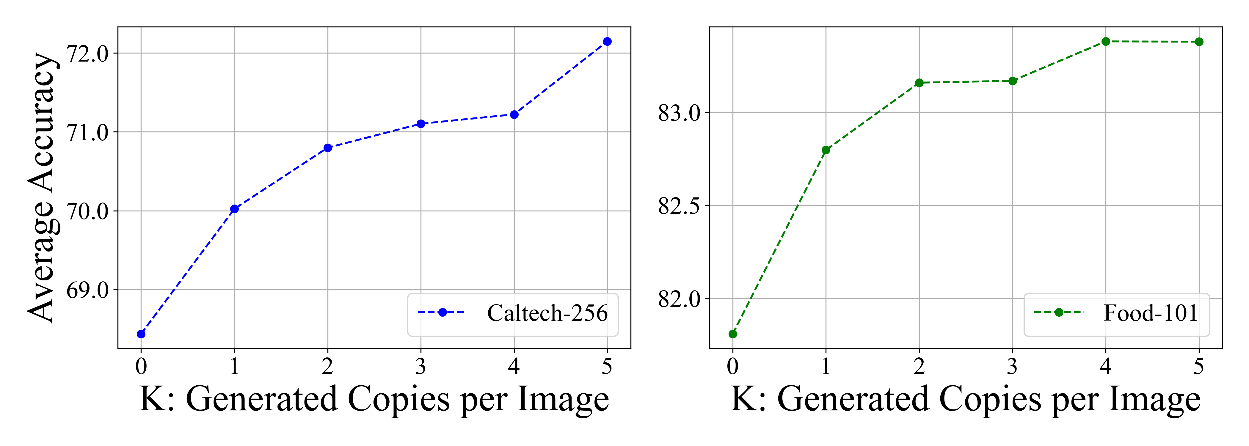
Figure 3: Average LFH accuracies of $N+1$ phases vs. number of generated copies per image (denoted by $K$) on Caltech-256 and Food-101. $K=0$ corresponds to the baseline without compression. Data augmentation with probability $p$ is applied, and $R$ real and $S$ synthetic exemplars are given to each class. In Caltech-256, $N=5$, $p=0.2$, $b=5$, $R=4$, and $S=18$; in Food-101, $N=5$, $p=0.3$, $b=20$, $R=18$, and $S=48$.

Method	Food-101			Places-100
	$b$=5	10	20	5	10	20
DER [47]	77.3	79.1	80.4	67.1	68.6	69.5
DER + ESCORT	80.1	81.3	83.2	69.6	70.4	71.3
Improvements	+2.8	+2.2	+2.8	+2.5	+1.8	+1.8

Table 4: Average LFH accuracies of $N+1$ phases of DER with and without ESCORT on Food-101 and Places-100 with different memory budgets $b$ units per class. Here $N=10$ for both datasets.

Different memory budgets. Due to data privacy and hardware limitations in real-world applications, the memory to store exemplars in CIL problems is often highly restricted. In these cases, whether our ESCORT is still able to provide the same effect has to be examined. We alter the memory budget $b$ in Food-101 and Places-100 and quantify the improvements in Tab. 4. It is remarkable that ESCORT consistently improves the accuracy with various memory budgets.

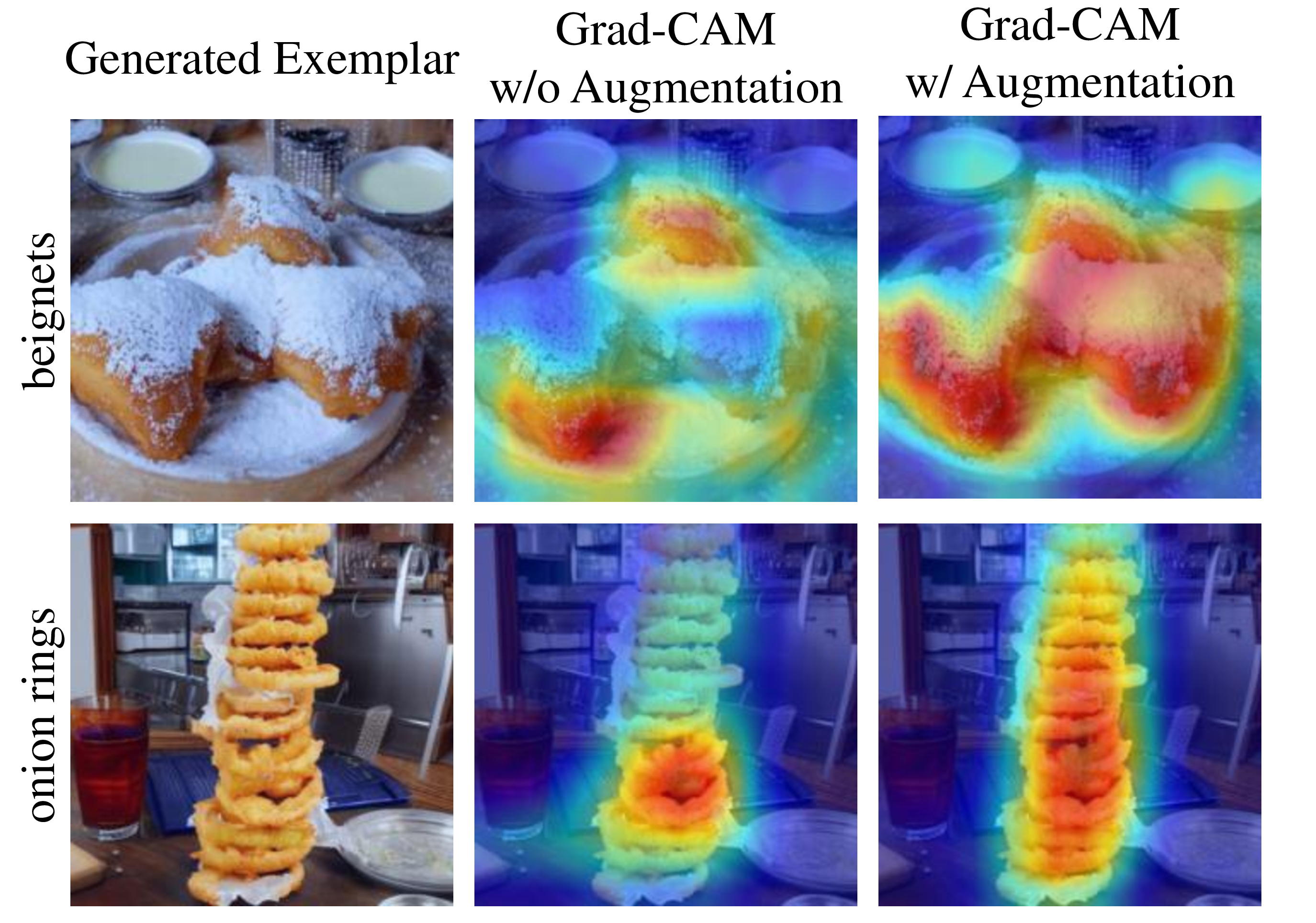
Figure 4: Two generated exemplars (left) from Food-101 with their Grad-CAM produced by the CIL model trained without diffusion-based data augmentation (middle) and with augmentation (right). The important activation regions given by the model trained with data augmentation capture the class objects much more accurately.

Grad-CAM visualization of generated exemplars. To verify if the class objects generated by ControlNet can be successfully identified by the CIL model, we use Grad-CAM [41] to detect the image region with the most importance to the classification decision. Displayed in Fig. 4 are two synthetic exemplars of Food-101 with their activation maps produced by a model trained without diffusion-based data augmentation and a model trained with augmentation. It is clear that the augmentation process is vital for the classification model to comprehensively detect generated objects. This ensures that the model can properly benefit from generated exemplars during training in subsequent stages.

5 Conclusion

In this paper, we propose an exemplar super-compression and regeneration approach, ESCORT, for replay-based class-incremental learning. ESCORT boosts the model performance by increasing the quantity and diversity of exemplars under a restricted memory budget. At the end of each incremental phase, selected images are compressed to visual and textual prompts, taking much less memory compared to RGB images. In subsequent stages, images of great diversity are regenerated from the prompts by the off-the-shelf ControlNet, a pre-trained diffusion model that doesn’t require fine-tuning or memory usage. To bridge the domain gap between real and generated exemplars, partial compression and diffusion-based data augmentation are proposed to let the model properly benefit from the synthetic exemplars. Experiment results demonstrate that our approach constantly improves the model performance by a large margin on various datasets and CIL settings.

Supplementary Materials

A Dataset Information

The information on the datasets used in our experiments is presented in Tab. S1. Caltech-256 has a generally smaller image size compared to the other two datasets.

B Data Preprocessing

The image preprocessing procedures are listed in Tab. S2 in PyTorch convention. Following FOSTER [45], we also leverage AutoAugment [9] in training for a fair comparison.

C Hyperparameters

The most important hyperparameters of ESCORT are the compressed proportion $\alpha$ and the augmentation probability $p$. As observed in [46], the best exemplar compression hyperparameters depend on the CIL setting. Therefore, we employ grid search in each setting to determine the optimal $\alpha$ and $p$, similar to what we do in Tab. 3.

Here, we report the hyperparameters adopted in our experiments. The $\alpha$ and $p$ that produce the results in Tab. 1 (LFH experiments) are presented in Tab. S3, while the $\alpha$ and $p$ that provide the results in Tab. 2 (LFS experiments) and Tab. 4 (budget experiments) are listed in Tab. S4.

In general, when budget $b=5$ memory units per class, taking $1$ out of each $5$ units (i.e., $\alpha=0.2$) to store edge maps is always optimal. When $b=10$ or $20$ units per class, a compressed proportion of $\alpha=0.1$ works best in most cases. For the augmentation probability, the optimal $p$ varies from $0.2$ to $0.4$ depending on the setting.

D Effect of Image Resizing

To resize an image with an original size of $h\times w$ into an edge map of size $H\times W$, there are two methods. One is to convert the image ($h\times w$) into edge map ($h\times w$) and have the edge map resized ($H\times W$) by nearest neighbor interpolation; the other one is to resize the image ($h\times w$) into an intermediate image ($H\times W$) by Lanczos interpolation first, and then extract the edge map ($H\times W$).

For some low-resolution images, it is beneficial to resize the image first and store a larger edge map, which captures more image details. Some memory is sacrificed; thus, the exemplar quantity is reduced, but we can gain exemplars with higher quality, as illustrated in the right column of Fig. S1.

Dataset	Caltech-256	Food-101	Places-100
# Classes	256	101	100
# Training images	21,436	75,750	300,000
# Training images/class (avg)	84	750	3,000
# Test images	75,472	25,250	10,000
# Test images/class (avg)	21	250	100
Median image size ($h\times w$)	289 $\times$ 300	512 $\times$ 512	512 $\times$ 683

Table S1: Detailed information of the three datasets, including number of classes, total number of training/test images, average number of training/test images per class, and median image size.

Training transformations	Test transformations
RandomResizedCrop(224),	Resize(256), CenterCrop(224),
RandomHorizontalFlip(),
ColorJitter(brightness=63/255),
ImageNetPolicy(),
ToTensor(),	ToTensor(),
Normalize(),	Normalize(),

Table S2: Training and test image transformations expressed in PyTorch convention. Normalization follows the traditional choice of mean ([0.485, 0.456, 0.406]) and standard deviation ([0.229, 0.224, 0.225]).

Hyperparameter	Caltech-256			Food-101			Places-100
	$N$=2	5	10	2	5	10	2	5	10
$\alpha$	0.2	0.2	0.2	0.1	0.15	0.1	0.1	0.1	0.1
$p$	0.2	0.2	0.2	0.4	0.3	0.4	0.4	0.4	0.4

Table S3: Hyperparameters to produce results of Tab. 1.

Hyperparameter	Caltech-256			Food-101			Places-100
	$N$=5	10	25	$b$=5	10	20	$b$=5	10	20
$\alpha$	0.2	0.2	0.2	0.2	0.1	0.1	0.2	0.1	0.1
$p$	0.4	0.4	0.3	0.3	0.3	0.4	0.4	0.4	0.4

Table S4: Hyperparameters to give results of Tab. 2 and Tab. 4.

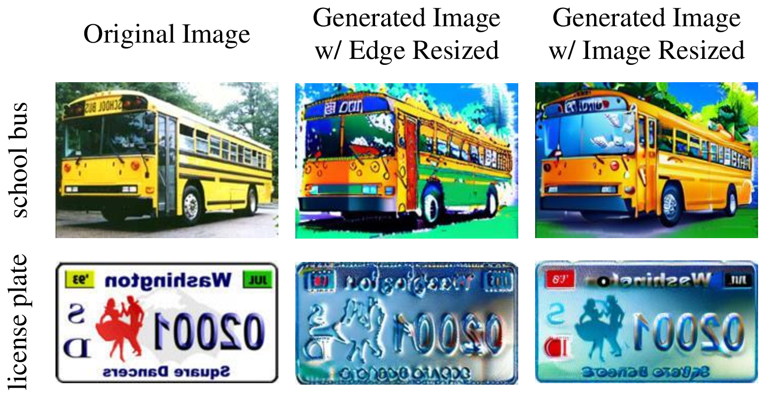
Figure S1: Two example images from Caltech-256 (left), their generated images with edge map resized (middle), and their generated images with image resized (right).

References

- Aljundi et al. [2017] Rahaf Aljundi, Punarjay Chakravarty, and Tinne Tuytelaars. Expert gate: Lifelong learning with a network of experts. In CVPR, pages 3366–3375, 2017.
- Aljundi et al. [2018] Rahaf Aljundi, Francesca Babiloni, Mohamed Elhoseiny, Marcus Rohrbach, and Tinne Tuytelaars. Memory aware synapses: Learning what (not) to forget. In ECCV, pages 139–154, 2018.
- Aljundi et al. [2019] Rahaf Aljundi, Min Lin, Baptiste Goujaud, and Yoshua Bengio. Gradient based sample selection for online continual learning. NeurIPS, 32, 2019.
- Bang et al. [2021] Jihwan Bang, Heesu Kim, YoungJoon Yoo, Jung-Woo Ha, and Jonghyun Choi. Rainbow memory: Continual learning with a memory of diverse samples. In CVPR, pages 8218–8227, 2021.
- Bossard et al. [2014] Lukas Bossard, Matthieu Guillaumin, and Luc Van Gool. Food-101–mining discriminative components with random forests. In ECCV, pages 446–461. Springer, 2014.
- Canny [1986] John F. Canny. A computational approach to edge detection. TPAMI, 8(6):679–698, 1986.
- Chaudhry et al. [2018] Arslan Chaudhry, Puneet K Dokania, Thalaiyasingam Ajanthan, and Philip HS Torr. Riemannian walk for incremental learning: Understanding forgetting and intransigence. In ECCV, pages 532–547, 2018.
- Chen and Liu [2018] Zhiyuan Chen and Bing Liu. Lifelong machine learning. Synthesis Lectures on Artificial Intelligence and Machine Learning, 12(3):1–207, 2018.
- Cubuk et al. [2019] Ekin D Cubuk, Barret Zoph, Dandelion Mane, Vijay Vasudevan, and Quoc V Le. Autoaugment: Learning augmentation strategies from data. In CVPR, pages 113–123, 2019.
- De Lange et al. [2019a] Matthias De Lange, Rahaf Aljundi, Marc Masana, Sarah Parisot, Xu Jia, Aleš Leonardis, Gregory Slabaugh, and Tinne Tuytelaars. A continual learning survey: Defying forgetting in classification tasks. arXiv, 1909.08383, 2019a.
- De Lange et al. [2019b] Matthias De Lange, Rahaf Aljundi, Marc Masana, Sarah Parisot, Xu Jia, Ales Leonardis, Gregory Slabaugh, and Tinne Tuytelaars. Continual learning: A comparative study on how to defy forgetting in classification tasks. arXiv, 1909.08383, 2019b.
- Douillard et al. [2020] Arthur Douillard, Matthieu Cord, Charles Ollion, Thomas Robert, and Eduardo Valle. Podnet: Pooled outputs distillation for small-tasks incremental learning. In ECCV, pages 86–102. Springer, 2020.
- Griffin et al. [2022] Gregory Griffin, Alex Holub, and Pietro Perona. Caltech 256, 2022.
- He et al. [2018] Chen He, Ruiping Wang, Shiguang Shan, and Xilin Chen. Exemplar-supported generative reproduction for class incremental learning. In BMVC, page 98, 2018.
- He et al. [2016] Kaiming He, Xiangyu Zhang, Shaoqing Ren, and Jian Sun. Deep residual learning for image recognition. In CVPR, pages 770–778, 2016.
- Ho et al. [2020] Jonathan Ho, Ajay Jain, and Pieter Abbeel. Denoising diffusion probabilistic models. In NeurIPS, 2020.
- Ho et al. [2022] Jonathan Ho, Chitwan Saharia, William Chan, David J Fleet, Mohammad Norouzi, and Tim Salimans. Cascaded diffusion models for high fidelity image generation. JMLR, 23(47):1–33, 2022.
- Hou et al. [2019] Saihui Hou, Xinyu Pan, Chen Change Loy, Zilei Wang, and Dahua Lin. Learning a unified classifier incrementally via rebalancing. In CVPR, pages 831–839, 2019.
- Hu et al. [2018] Wenpeng Hu, Zhou Lin, Bing Liu, Chongyang Tao, Zhengwei Tao, Jinwen Ma, Dongyan Zhao, and Rui Yan. Overcoming catastrophic forgetting for continual learning via model adaptation. In ICLR, 2018.
- Iscen et al. [2020] Ahmet Iscen, Jeffrey Zhang, Svetlana Lazebnik, and Cordelia Schmid. Memory-efficient incremental learning through feature adaptation. In ECCV, pages 699–715. Springer, 2020.
- Isele and Cosgun [2018] David Isele and Akansel Cosgun. Selective experience replay for lifelong learning. In AAAI, 2018.
- Kirkpatrick et al. [2017] James Kirkpatrick, Razvan Pascanu, Neil Rabinowitz, Joel Veness, Guillaume Desjardins, Andrei A Rusu, Kieran Milan, John Quan, Tiago Ramalho, Agnieszka Grabska-Barwinska, et al. Overcoming catastrophic forgetting in neural networks. PNAS, 114(13):3521–3526, 2017.
- Lee et al. [2017] Sang-Woo Lee, Jin-Hwa Kim, Jaehyun Jun, Jung-Woo Ha, and Byoung-Tak Zhang. Overcoming catastrophic forgetting by incremental moment matching. NeurIPS, 30, 2017.
- Li and Hoiem [2017] Zhizhong Li and Derek Hoiem. Learning without forgetting. TPAMI, 40(12):2935–2947, 2017.
- Liu et al. [2020] Yaoyao Liu, Yuting Su, An-An Liu, Bernt Schiele, and Qianru Sun. Mnemonics training: Multi-class incremental learning without forgetting. In CVPR, pages 12245–12254, 2020.
- Liu et al. [2021a] Yaoyao Liu, Bernt Schiele, and Qianru Sun. Adaptive aggregation networks for class-incremental learning. In CVPR, pages 2544–2553, 2021a.
- Liu et al. [2021b] Yaoyao Liu, Bernt Schiele, and Qianru Sun. Rmm: Reinforced memory management for class-incremental learning. NeurIPS, 34:3478–3490, 2021b.
- Liu et al. [2021c] Yaoyao Liu, Qianru Sun, Xiangnan He, An-An Liu, Yuting Su, and Tat-Seng Chua. Generating face images with attributes for free. TNNLS, 32(6):2733–2743, 2021c.
- Liu et al. [2023a] Yaoyao Liu, Yingying Li, Bernt Schiele, and Qianru Sun. Online hyperparameter optimization for class-incremental learning. In AAAI, pages 8906–8913, 2023a.
- Liu et al. [2023b] Yaoyao Liu, Bernt Schiele, Andrea Vedaldi, and Christian Rupprecht. Continual detection transformer for incremental object detection. In CVPR, pages 23799–23808, 2023b.
- lllyasviel [2023] lllyasviel. ControlNet. https://github.com/lllyasviel/ControlNet, 2023.
- Lopez-Paz and Ranzato [2017] David Lopez-Paz and Marc’Aurelio Ranzato. Gradient episodic memory for continual learning. In NIPS, pages 6467–6476, 2017.
- Luo et al. [2023] Zilin Luo, Yaoyao Liu, Bernt Schiele, and Qianru Sun. Class-incremental exemplar compression for class-incremental learning. In CVPR, pages 11371–11380, 2023.
- McCloskey and Cohen [1989] Michael McCloskey and Neal J Cohen. Catastrophic interference in connectionist networks: The sequential learning problem. In Psychology of learning and motivation, pages 109–165. Elsevier, 1989.
- Petit et al. [2023] Grégoire Petit, Adrian Popescu, Hugo Schindler, David Picard, and Bertrand Delezoide. Fetril: Feature translation for exemplar-free class-incremental learning. In WACV, pages 3911–3920, 2023.
- Pham et al. [2021] Quang Pham, Chenghao Liu, and Steven Hoi. Dualnet: Continual learning, fast and slow. NeurIPS, 34:16131–16144, 2021.
- Prabhu et al. [2020] Ameya Prabhu, Philip HS Torr, and Puneet K Dokania. Gdumb: A simple approach that questions our progress in continual learning. In ECCV, 2020.
- Ratcliff [1990] R. Ratcliff. Connectionist models of recognition memory: Constraints imposed by learning and forgetting functions. Psychological Review, 97:285–308, 1990.
- Rebuffi et al. [2017] Sylvestre-Alvise Rebuffi, Alexander Kolesnikov, Georg Sperl, and Christoph H Lampert. icarl: Incremental classifier and representation learning. In CVPR, pages 2001–2010, 2017.
- Rombach et al. [2022] Robin Rombach, Andreas Blattmann, Dominik Lorenz, Patrick Esser, and Björn Ommer. High-resolution image synthesis with latent diffusion models. In CVPR, pages 10684–10695, 2022.
- Selvaraju et al. [2017] Ramprasaath R Selvaraju, Michael Cogswell, Abhishek Das, Ramakrishna Vedantam, Devi Parikh, and Dhruv Batra. Grad-cam: Visual explanations from deep networks via gradient-based localization. In ICCV, pages 618–626, 2017.
- Shin et al. [2017] Hanul Shin, Jung Kwon Lee, Jaehong Kim, and Jiwon Kim. Continual learning with deep generative replay. NeurIPS, 30, 2017.
- Singer et al. [2022] Uriel Singer, Adam Polyak, Thomas Hayes, Xi Yin, Jie An, Songyang Zhang, Qiyuan Hu, Harry Yang, Oron Ashual, Oran Gafni, et al. Make-a-video: Text-to-video generation without text-video data. arXiv preprint arXiv:2209.14792, 2022.
- Villegas et al. [2022] Ruben Villegas, Mohammad Babaeizadeh, Pieter-Jan Kindermans, Hernan Moraldo, Han Zhang, Mohammad Taghi Saffar, Santiago Castro, Julius Kunze, and Dumitru Erhan. Phenaki: Variable length video generation from open domain textual description. arXiv preprint arXiv:2210.02399, 2022.
- Wang et al. [2022a] Fu-Yun Wang, Da-Wei Zhou, Han-Jia Ye, and De-Chuan Zhan. Foster: Feature boosting and compression for class-incremental learning. In ECCV, pages 398–414. Springer, 2022a.
- Wang et al. [2022b] Liyuan Wang, Xingxing Zhang, Kuo Yang, Longhui Yu, Chongxuan Li, Lanqing Hong, Shifeng Zhang, Zhenguo Li, Yi Zhong, and Jun Zhu. Memory replay with data compression for continual learning. arXiv preprint arXiv:2202.06592, 2022b.
- Yan et al. [2021] Shipeng Yan, Jiangwei Xie, and Xuming He. Der: Dynamically expandable representation for class incremental learning. In CVPR, pages 3014–3023, 2021.
- Yoon et al. [2017] Jaehong Yoon, Eunho Yang, Jeongtae Lee, and Sung Ju Hwang. Lifelong learning with dynamically expandable networks. arXiv preprint arXiv:1708.01547, 2017.
- Zenke et al. [2017] Friedemann Zenke, Ben Poole, and Surya Ganguli. Continual learning through synaptic intelligence. In ICML, pages 3987–3995. PMLR, 2017.
- Zhang et al. [2023a] Lvmin Zhang, Anyi Rao, and Maneesh Agrawala. Adding conditional control to text-to-image diffusion models. In ICCV, pages 3836–3847, 2023a.
- Zhang et al. [2023b] Yixiao Zhang, Xinyi Li, Huimiao Chen, Alan L. Yuille, Yaoyao Liu, and Zongwei Zhou. Continual learning for abdominal multi-organ and tumor segmentation. In MICCAI, pages 35–45. Springer, 2023b.
- Zhao et al. [2020] Bowen Zhao, Xi Xiao, Guojun Gan, Bin Zhang, and Shu-Tao Xia. Maintaining discrimination and fairness in class incremental learning. In CVPR, pages 13208–13217, 2020.
- Zhou et al. [2016] Bolei Zhou, Aditya Khosla, Agata Lapedriza, Antonio Torralba, and Aude Oliva. Places: An image database for deep scene understanding. arXiv preprint arXiv:1610.02055, 2016.
- Zhou et al. [2022] Da-Wei Zhou, Qi-Wei Wang, Han-Jia Ye, and De-Chuan Zhan. A model or 603 exemplars: Towards memory-efficient class-incremental learning. arXiv preprint arXiv:2205.13218, 2022.
- Zhou et al. [2023] Da-Wei Zhou, Fu-Yun Wang, Han-Jia Ye, and De-Chuan Zhan. Pycil: a python toolbox for class-incremental learning. SCIENCE CHINA Information Sciences, 66(9):197101–, 2023.
- Zhu et al. [2021] Fei Zhu, Xu-Yao Zhang, Chuang Wang, Fei Yin, and Cheng-Lin Liu. Prototype augmentation and self-supervision for incremental learning. In CVPR, pages 5871–5880, 2021.