Accelerating Level-Value Adjustment for the Polyak Stepsize

Abstract

The Polyak stepsize formula has been widely used for convex optimization. However, stepsize computations require the generally unknown optimal value. Dynamic estimations of the optimal value are thus usually needed. In this paper, guided by a decision-based procedure through a novel easy-to-solve “Polyak Stepsize Violation Detector” (PSVD) linear constraint satisfaction problem, a series of level values is constructed to successively estimate the optimal value to guarantee convergence for subgradient as well as for approximate subgradient methods. Through a series of empirical tests of convex optimization problems with diverse characteristics, we illustrate the practical advantages of our approach as compared to existing methods.

Keywords Convex Optimization  $\cdot$ Non-Smooth Optimization  $\cdot$ Polyak Stepsize  $\cdot$ Subgradient Method  $\cdot$ Approximate Subgradient Method

1 Introduction

This paper focuses on convex optimization problems, which are formally formulated as:

$$\underset{x}{\text{minimize}} f(x), x\in\mathcal{X}\subseteq\mathbb{R}^{n},$$ subject to (1)

where $f:\mathbb{R}^{n}\xrightarrow{}\mathbb{R}$ is a convex non-smooth objective function, and $\mathcal{X}$ is a closed, nonempty, and convex subset of $\mathbb{R}^{n}$. The optimal value is denoted as $f^{\star}\equiv\inf_{x\in\mathcal{X}}f(x)$ and is assumed to be bounded from below. An optimal set is defined as $\mathcal{X}^{\star}=\left\{x\in\mathcal{X}\mid f(x)=f^{\star}\right\}$ and is assumed to be non-empty.

Problems (1) appear in several contexts such as Lagrangian Relaxation whereby non-smooth convex dual functions are optimized [22, 14, 4, 5], approximation and fitting [16, 3], and support vector machine [17], and convex regression [11, 12]. Subgradient methods have been used to optimize (1) and involve taking a series of steps $s^{k}$ along subgradient directions $g^{k}$ as:

$$x^{k+1}=P_{\mathcal{X}}\left(x^{k}-s^{k}\cdot g^{k}\right),$$ (2)

where $P_{\mathcal{X}}$ is the projection onto $\mathcal{X}$, $s^{k}$ is a positive stepsize and $g^{k}$ is the subgradient of $f(\cdot)$ at $x^{k}$ that satisfies

$$f(x)\geq f(x^{k})+\big{(}g^{k}\big{)}^{T}\cdot(x-x^{k}),\forall x\in\mathcal{X}.$$ (3)

Throughout this paper, we assume that subgradients are bounded. Boundedness of Subgradients. There exists a scalar $C$, such that

$$\|g^{k}\|\leq C,\forall k.$$ (4)

Within (4) and thereafter in the paper, the standard Euclidean norm will be used. Assumption 3 is satisfied if, for example, $f(\cdot)$ satisfies the Lipschitz condition [2].

The dynamic stepsize introduced by Polyak in [18], has been widely used [10, 14, 12, 15]. The key idea behind is as follows. From (3) and the non-expansive property of $P_{\mathcal{X}}$, a classical result of subgradient methods can be derived as

$$\left\|x^{k+1}-x^{\star}\right\|^{2}-\left\|x^{k}-x^{\star}\right\|^{2}\leq-2s^{k}\left(f\left(x^{k}\right)-f^{\star}\right)+\left(s^{k}\right)^{2}\left\|g^{k}\right\|^{2},$$ (5)

where $x^{\star}\in\mathcal{X}^{\star}$ (see chapter 7.5 of [2]). With the Polyak stepsize

$$s^{k}=\gamma\cdot\frac{f(x^{k})-f^{\star}}{\big{\|}g^{k}\big{\|}^{2}},0<\gamma<\bar{\gamma}<2,$$ (6)

the right-hand side of (5) is negative, and $x^{k}$ strictly approaches and converges to an optimal solution. Moreover, under additional requirements on “sharpness” of $f(\cdot)$ as well as Lipschitz conditions, a convergence rate result has been derived as $\|x^{k+1}-x^{\star}\|\leq r\cdot\|x^{k}-x^{\star}\|$ with $r<1$ (see [18, 19]).

The primary challenge in employing the Polyak stepsize (6) is that, in most cases, the knowledge of the optimal value $f^{\star}$ is unavailable. To overcome this difficulty, $f^{\star}$ is generally replaced with a level value $\bar{f}_{k}$ (an estimate of $f^{\star}$) as:

$$s^{k}=\gamma\cdot\frac{f\left(x^{k}\right)-\bar{f}_{k}}{\left\|g^{k}\right\|^{2}},0<\gamma<\bar{\gamma}<2.$$ (7)

To guarantee convergence, $\bar{f}_{k}$ needs to be dynamically adjusted. In the following, the key ideas of two level-adjustment approaches [10, 5] are summarized.

Path-Based Level Adjustment. The path-based level adjustment approach was developed in [6, 10] and has been used in various subgradient methods [14, 13]. In the approach, the level is determined by offsetting the best function value obtained by $\delta^{k}$, which is adaptively decreased. Specifically, if the function value is sufficiently reduced, then the level value is “appropriate,” and $\delta^{k}$ is kept unchanged. Otherwise, the length of the path traversed by the solutions exceeds a predetermined value $B$, an oscillation of solution is detected, and $\delta^{k}$ is decreased. While the approach has been proven to converge, the selection of the hyperparameters (e.g., the value of $B$ and $\delta^{0}$) plays a crucial role in the performance of the approach and is generally problem-dependent.

Decision-Guided Level Adjustment. A decision-based level adjustment approach was recently developed in [5], where level values always underestimate $f^{\star}$ (for minimization problems such as (1)). The key idea is to detect when a solution “moves away” from $x^{\star}$. Suppose $x^{k_{j}}$ is updated per (2) with $s^{k_{j}}$ calculated based on (7) with a level value of $\bar{f}_{k_{j}}$. If the level value is “appropriate," such that $s^{k_{j}}$ satisfies the Polyak formula (6), then $x^{k_{j}+1}$ will get closer to $x^{\star}\in\mathcal{X}^{\star}$ as

$$\left\|x^{\star}-x^{k_{j}+1}\right\|^{2}\leq\left\|x^{\star}-x^{k_{j}}\right\|^{2}.$$ (8)

Conversely, if (8) is violated by $x^{k_{j}}$ and $x^{k_{j}+1}$, then the stepsize is “too large” such that the Polyak formula (6) is violated, and an adjustment of the previous level value is required. To operationalize the above idea, the following “Solution-Divergence Detector” (SDD) constraint satisfaction problem was established to trigger the level adjustment:

$$\left\{\begin{array}[]{c}\begin{aligned} \left\|x-x^{k_{j}+1}\right\|^{2}&\leq\left\|x-x^{k_{j}}\right\|^{2},\\ \left\|x-x^{k_{j}+2}\right\|^{2}&\leq\left\|x-x^{k_{j}+1}\right\|^{2},\\ &\vdots\\ \left\|x-x^{k_{j}+n}\right\|^{2}&\leq\left\|x-x^{k_{j}+n-1}\right\|^{2},\\ \end{aligned}\end{array}\right.$$ (9)

where $x\in\mathbb{R}^{n}$ is the decision variable and $\{x^{k}\}_{k=k_{j}}^{k_{j}+n}$ are solutions obtained by using (7). The infeasibility of (9) indicates that $\{x^{k}\}_{k=k_{j}}^{k_{j}+n}$ does not approach any solution, including $x^{\star}\in\mathcal{X}^{\star}$. This triggers an adjustment of the level value (for specific details, see [5, Eq. (20)]). If the SDD problem (9) is feasible, then a new inequality $\left\|x-x^{k_{j}+n+1}\right\|^{2}\leq\left\|x-x^{k_{j}+n}\right\|^{2}$ is appended into (9), which is checked for feasibility again in the next iteration. The major advantage of the above decision-guided procedure is its problem-agnostic as well as hyperparameter-adjustment-free nature. However, there are three major difficulties:

1. While the infeasibility of (9) indicates that $\{x^{k}\}_{k=k_{j}}^{k_{j}+n}$ do not approach $x^{\star}$, the feasibility of (9), however, does not indicate that $\{x^{k}\}_{k=k_{j}}^{k_{j}+n}$ approach $x^{\star}$. Consequently, the algorithm may require multiple additional iterations before adjusting the level;

2. Convergence of the approach was not established in [5]; and

3. The SDD problem (9) involves quadratic terms. When the problem (1) has constraints (i.e., $\mathcal{X}\subset\mathbb{R}^{n}$), the SDD problem (9) may not be able to equivalently transform into a linear one, and checking (9) may be costly.

In this paper, we develop a novel decision-guided level adjustment approach based on the idea behind that of [5] while overcoming the major difficulties listed above. Specifically, our corresponding three contributions are as follows:

1. A “Polyak Stepsize Violation Detector" (PSVD) problem is developed, which is used to trigger the level adjustment. The PSVD problem is shown to be “tighter" than the SDD problem (9), and the level adjustment of [5] is thus accelerated;

2. Convergence of subgradient methods with PSVD is rigorously proven;

3. The PSVD problem is a linear constraint satisfaction problem. Its feasibility can be checked in a computationally efficient manner; and

4. The results are generalized for approximate subgradient methods.

As will be detailed in Section 2, the novel approach, which we refer to as the Polyak Stepsize with Accelerated Decision-guided Level Adjustment (PSADLA), offers an accelerated convergence as compared to previous methods. In Section 3, PSADLA enables the use of approximate subgradients under easy-to-satisfy convergence conditions, leading to much reduced computational effort. The new method is particularly applicable to convex optimization problems with additive objectives arising in machine learning and to dual problems arising within Lagrangian Relaxation for discrete programming; the specialized form of approximate subgradients is akin to “surrogate subgradients" in previous studies [22, 5]. In Section 4, the method’s faster convergence is empirically demonstrated through a variety of convex problems as compared to previous methods. Conclusions are drawn in Section 5.

2 Polyak Stepsize with Accelerated Decision-Guided Level Adjustment (PSADLA) for Subgradient Methods

In this section, the PSADLA approach is developed for subgradient methods. Our level-adjustment approach detects Polyak stepsize violations directly using a novel “Polyak Stepsize Violation Detector" (PSVD) problem. In subsection 2.1, the key ideas behind the PSVD problem and the level adjustment formula are highlighted, followed by a pseudo-code of the algorithm. In subsection 2.2, the convergence results are established.

2.1 Polyak Stepsize Violation Detector Problem for Level Adjustment

In this subsection, the key idea of PSVD is presented after the two supporting Lemmas 2.1 and 2.1.

Let $x^{k}$ be a solution, $g^{k}$ be a subgradient of $f(\cdot)$ at $x^{k}$ and $x^{\star}\in\mathcal{X}^{\star}$. If stepsize $s^{k}$ does not satisfy

$$\left(g^{k}\right)^{T}x^{\star}\leq\left(g^{k}\right)^{T}x^{k}-\frac{1}{\bar{\gamma}}s^{k}\left\|g^{k}\right\|^{2},$$ (10)

then

$$s^{k}>\bar{\gamma}\cdot\frac{f\left(x^{k}\right)-f^{\star}}{\left\|g^{k}\right\|^{2}}.$$ (11)

Proof The proof will follow by contradiction. Assume that (10) is violated but $s^{k}\leq\bar{\gamma}\cdot\frac{f\left(x^{k}\right)-f^{\star}}{\left\|g^{k}\right\|^{2}}$. From the latter, the following inequality holds:

$$\frac{1}{\bar{\gamma}}s^{k}\left\|g^{k}\right\|^{2}\leq f\left(x^{k}\right)-f^{\star}.$$ (12)

By using (3), the above inequality can be further written as

$$\frac{1}{\bar{\gamma}}s^{k}\left\|g^{k}\right\|^{2}\leq f\left(x^{k}\right)-f^{\star}\leq\big{(}g^{k}\big{)}^{T}\cdot(x^{k}-x^{\star}),$$ (13)

which means that (10) is satisfied – a contradiction. $\square$

The premise behind the above Lemma is that $s^{k}$ is set per (7) with “inappropriately low” level $\bar{f}_{k}$ so that $s^{k}$ violates the Polyak formula (6). The violation of (6) is detected through the violation of (10), which also triggers the recalculation of the level value as explained in the following Lemma.

Let $x^{k}$ be a solution and $g^{k}$ be a subgradient of $f(\cdot)$ at $x^{k}$. Stepsize $s^{k}$ is calculated by using a level value $\bar{f_{k}}$ ($\bar{f_{k}}<f^{\star}$) per (7). If inequality (10) is not satisfied, then a scalar $\bar{f}^{\prime}$ defined as

$$\bar{f}^{\prime}=\frac{\gamma}{\bar{\gamma}}\bar{f_{k}}+\left(1-\frac{\gamma}{\bar{\gamma}}\right)f\left(x^{k}\right)$$ (14)

is a tighter estimate of $f^{\star}$ such that

$$\bar{f_{k}}<\bar{f}^{\prime}<f^{\star}.$$ (15)

Proof Part 1: $\bar{f_{k}}<\bar{f}^{\prime}:$ Within (14), $\bar{f}^{\prime}$ is a convex combination of $\bar{f}_{k}$ and $f\left(x^{k}\right)$. The function value $f\left(x^{k}\right)$ is always larger than the level value $\bar{f}_{k}$. Therefore, $\bar{f}^{\prime}$ is larger than $\bar{f}_{k}$.

Part 2: $\bar{f}^{\prime}<f^{\star}:$ Based on Lemma 2.1, the violation of (10) implies the satisfaction of (11). After replacing $s^{k}$ in (11) with (7), the following holds:

$$\gamma\cdot\frac{f\left(x^{k}\right)-\bar{f}_{k}}{\left\|g^{k}\right\|^{2}}>\bar{\gamma}\cdot\frac{f\left(x^{k}\right)-f^{\star}}{\left\|g^{k}\right\|^{2}}.$$ (16)

After canceling $\|g^{k}\|^{2}$ and rearranging the remaining terms, the above inequality can be equivalently rewritten as

$$f^{\star}>f\left(x^{k}\right)-\frac{\gamma}{\bar{\gamma}}f\left(x^{k}\right)+\frac{\gamma}{\bar{\gamma}}\bar{f}_{k},$$ (17)

where the right-hand side is $\bar{f}^{\prime}$. $\square$

The above two Lemmas demonstrate that if the violation of (10) is detected, then the Polyak stepsize is violated, and a new level value can be generated by the convex combination (14). However, checking (10) is impractical since $x^{\star}$ are unknown. In the following Theorem 2.1, a novel “Polyak Stepsize Violation Detector" (PSVD) constraint satisfaction problem is established without requiring $x^{\star}$.

Suppose that $\{x^{k}\}_{k=k_{j}}^{k_{j}+n-1}$ are iteratively generated per (2) by using subgradients $\{g^{k}\}_{k=k_{j}}^{k_{j}+n-1}$ and stepsizes $\{s^{k}\}_{k=k_{j}}^{k_{j}+n-1}$ calculated per (7) based on underestimating level values $\{\bar{f}_{k}\}_{k=k_{j}}^{k_{j}+n-1}$. If the following PSVD constraint satisfaction problem (with $x\in\mathbb{R}^{n}$ being the decision variable)

$$\left\{\begin{array}[]{c}\begin{aligned} \left(g^{k_{j}}\right)^{T}x&\leq\left(g^{k_{j}}\right)^{T}x^{k_{j}}-\frac{1}{\bar{\gamma}}s^{k_{j}}\left\|g^{k_{j}}\right\|^{2},\\ \left(g^{k_{j}+1}\right)^{T}x&\leq\left(g^{k_{j}+1}\right)^{T}x^{k_{j}+1}-\frac{1}{\bar{\gamma}}s^{k_{j}+1}\left\|g^{k_{j}+1}\right\|^{2},\\ &\vdots\\ \left(g^{k_{j}+n-1}\right)^{T}x&\leq\left(g^{k_{j}+n-1}\right)^{T}x^{k_{j}+n-1}-\frac{1}{\bar{\gamma}}s^{k_{j}+n-1}\left\|g^{k_{j}+n-1}\right\|^{2},\end{aligned}\end{array}\right.$$ (18)

does not admit a feasible solution, then $\exists\kappa\in\{k_{j},k_{j}\!+\!1,...,k_{j}\!+\!n\!-\!1\}$, such that

$$s^{\kappa}>\bar{\gamma}\cdot\frac{f\left(x^{\kappa}\right)-f^{\star}}{\left\|g^{\kappa}\right\|^{2}}.$$ (19)

Accordingly, a new level value $\bar{f}_{k_{j}+n}$ can be generated as

$$\bar{f}_{k_{j}+n}=\frac{\gamma}{\bar{\gamma}}\bar{f}_{k_{j}+n-1}+\left(1-\frac{\gamma}{\bar{\gamma}}\right)\min_{\kappa\in\{k_{j},k_{j}+1,...,k_{j}+n-1\}}\left\{f\left(x^{\kappa}\right)\right\},$$ (20)

which is a tighter level as compared to $\bar{f}_{k_{j}+n-1}$ such that $\bar{f}_{k_{j}+n-1}\!<\!\bar{f}_{k_{j}+n}\!<\!f^{\star}$.

Proof Inequality (19) follows from Lemma 2.1. If (18) has no feasible solution, then no $x^{\star}$ in $\mathcal{X}^{\star}$ satisfies (18). Consequently, there must be a $\kappa$ in $\{k_{j},k_{j}+1,...,k_{j}+n-1\}$ for which the following inequality holds:

$$\left(g^{\kappa}\right)^{T}x^{\star}>\left(g^{\kappa}\right)^{T}x^{\kappa}-\frac{1}{\bar{\gamma}}s^{\kappa}\left\|g^{\kappa}\right\|^{2}.$$ (21)

According to Lemma 2.1, the Polyak formula is violated and (19) is satisfied. Based on Lemma 2.1, the following inequality holds

$$\frac{\gamma}{\bar{\gamma}}\bar{f}_{k_{j}+n-1}+\left(1-\frac{\gamma}{\bar{\gamma}}\right)f\left(x^{\kappa}\right)<f^{\star},$$ (22)

and therefore, we must have

$$\bar{f}_{k_{j}+n}=\frac{\gamma}{\bar{\gamma}}\bar{f}_{k_{j}+n-1}+\left(1-\frac{\gamma}{\bar{\gamma}}\right)\min_{\kappa\in\{k_{j},k_{j}+1,...,k_{j}+n-1\}}\left\{f\left(x^{\kappa}\right)\right\}<f^{\star}.$$ (23)

Since $\gamma<\bar{\gamma}$, (20) is a convex combination. The level value $\bar{f}_{k_{j}+n-1}$ is less than $\min_{\kappa\in\{k_{j},k_{j}+1,...,k_{j}+n-1\}}\left\{f\left(x^{\kappa}\right)\right\}$, and we thus have $\bar{f}_{k_{j}+n}>\bar{f}_{k_{j}+n-1}$. $\square$

During the iterative procedure, the feasibility of the PSVD problem (18) is checked periodically; each time the problem is infeasible, a new level value is calculated. Problem (18) is linear and can thus be handled by LP methods. In the following, the “tightness" of PSVD and SDD problems (9) is compared.

If the PSVD problem (18) has a feasible solution $x^{\prime}\in\mathbb{R}^{n}$, then $x^{\prime}$ is also feasible to the following constraint satisfaction problem (with $x\in\mathbb{R}^{n}$ being the decision variable)

$$\left\{\begin{aligned} \left\|x-x^{k_{j}+1}\right\|^{2}-\left\|x-x^{k_{j}}\right\|^{2}&\leq\left(1-\frac{2}{\bar{\gamma}}\right)\left(s^{k_{j}}\right)^{2}\left\|g^{k_{j}}\right\|^{2},\\ \left\|x-x^{k_{j}+2}\right\|^{2}-\left\|x-x^{k_{j}+1}\right\|^{2}&\leq\left(1-\frac{2}{\bar{\gamma}}\right)\left(s^{k_{j}+1}\right)^{2}\left\|g^{k_{j}+1}\right\|^{2},\\ \vdots&\\ \left\|x-x^{k_{j}+n}\right\|^{2}-\left\|x-x^{k_{j}+n-1}\right\|^{2}&\leq\left(1-\frac{2}{\bar{\gamma}}\right)\left(s^{k_{j}+n-1}\right)^{2}\left\|g^{k_{j}+n-1}\right\|^{2}.\end{aligned}\right.$$ (24)

Proof Consider the first inequalities of (18) and (24). The first inequality of (18) can equivalently be written as

$$-2s^{k_{j}}\left(x^{k_{j}}-x\right)^{T}g^{k_{j}}+\left(s^{k_{j}}\right)^{2}\left\|g^{k_{j}}\right\|^{2}\leq\left(1-\frac{2}{\bar{\gamma}}\right)\left(s^{k_{j}}\right)^{2}\left\|g^{k_{j}}\right\|^{2}.$$ (25)

By using the non-expansive property of $P_{\mathcal{X}}$, the following inequality holds:

$$\left\|x^{k_{j}+1}\!-\!x\right\|^{2}\!-\!\left\|x^{k_{j}}\!-\!x\right\|^{2}\leq-2s^{k_{j}}\left(x^{k_{j}}\!-\!x\right)^{T}g^{k_{j}}\!+\!\left(s^{k_{j}}\right)^{2}\left\|g^{k_{j}}\right\|^{2},\forall x\in\mathcal{X}.$$ (26)

The right-hand side of (26) is the same as that of (25). If (25) holds for some $x^{\prime}$, then we must have

$$\left\|x^{k_{j}+1}-x^{\prime}\right\|^{2}-\left\|x^{k_{j}}-x^{\prime}\right\|^{2}\leq\left(1-\frac{2}{\bar{\gamma}}\right)\left(s^{k_{j}}\right)^{2}\left\|g^{k_{j}}\right\|^{2},$$ (27)

which implies that $x^{\prime}$ satisfies the first inequality of (24). The results hold for other inequalities. $\square$

The left-hand side of (24) is the same as that of (9) while the right-hand side of (24) is negative. Therefore, problem (24) imposes stricter restrictions than (9).

The entire algorithm is presented below.

Algorithm 2.1: Subgradient Method with PSADLA

Step 1 (Initialization) Initialize $x^{0}$, $\bar{f}_{0}$ as a value less than $f^{\star}$, $\gamma$ and $\bar{\gamma}$ such that $0<\gamma<\bar{\gamma}<2$, and $k$ as zero.

Step 2 (Update) Update solutions as $x^{k+1}=P_{\mathcal{X}}\left(x^{k}-s^{k}\cdot g^{k}\right)$, where the stepsize calculated as $s^{k}=\gamma\cdot\frac{f\left(x^{k}\right)-\bar{f}_{k}}{\left\|g^{k}\right\|^{2}}$.

Step 3 (Level Adjustment) Append $\left(g^{k}\right)^{T}x\leq\left(g^{k}\right)^{T}x^{k}-\frac{1}{\bar{\gamma}}s^{k}\left\|g^{k}\right\|^{2}$ to the PSVD problem (18). If the problem does not admit any feasible solution, a new level $\bar{f}_{k+1}$ is generated per (20) and all inequalities from the PSVD problem are removed; otherwise, the level value is kept at $\bar{f}_{k+1}=\bar{f}_{k}$.

Step 4 (Stopping Criteria Checking) If stopping criteria, such as a difference between the best function value so far ($\min_{\kappa=1,...,k}f(x^{\kappa})$) and the current level value ($\bar{f}_{k}$), falls below a small predefined scalar $\varsigma$, or if the number of iterations/CPU time limit is reached, then stop. If these conditions are not met, increment $k$ by 1 and go to Step 2.

2.2 Convergence Proof

In this subsection, the convergence of the above algorithm is proven. To this end, a supporting Lemma 2.2 stating that the PSVD problem (18) becomes infeasible infinitely often as $k\rightarrow\infty$ will be proven first.

Within the subgradient method with PSADLA, the PSVD problem (18) becomes infeasible infinitely often as $k\rightarrow\infty$. Proof The proof will follow by contradiction. Assume that after iteration $k^{\prime}$, the problem (18) always has a feasible solution $x^{\prime}\in\mathbb{R}^{n}$, i.e., for any $k>k^{\prime}$, the following inequalities hold

$$\left\{\begin{aligned} \left(g^{k^{\prime}}\right)^{T}x^{\prime}&\leq\left(g^{k^{\prime}}\right)^{T}x^{k^{\prime}}-\frac{1}{\bar{\gamma}}s^{k^{\prime}}\left\|g^{k^{\prime}}\right\|^{2},\\ \left(g^{k^{\prime}+1}\right)^{T}x^{\prime}&\leq\left(g^{k^{\prime}+1}\right)^{T}x^{k^{\prime}+1}-\frac{1}{\bar{\gamma}}s^{k^{\prime}+1}\left\|g^{k^{\prime}+1}\right\|^{2},\\ &\vdots\\ \left(g^{k}\right)^{T}x^{\prime}&\leq\left(g^{k}\right)^{T}x^{k}-\frac{1}{\bar{\gamma}}s^{k}\left\|g^{k}\right\|^{2}.\\ \end{aligned}\right.$$ (28)

Based on Proposition 2.1, $x^{\prime}$ is also feasible to problem (24), i.e.,

$$\left\{\begin{aligned} \left\|x^{\prime}-x^{k^{\prime}+1}\right\|^{2}-\left\|x^{\prime}-x^{k^{\prime}}\right\|^{2}&\leq\left(1-\frac{2}{\bar{\gamma}}\right)\left(s^{k^{\prime}}\right)^{2}\left\|g^{k^{\prime}}\right\|^{2},\\ \left\|x^{\prime}-x^{k^{\prime}+2}\right\|^{2}-\left\|x^{\prime}-x^{k^{\prime}+1}\right\|^{2}&\leq\left(1-\frac{2}{\bar{\gamma}}\right)\left(s^{k^{\prime}+1}\right)^{2}\left\|g^{k^{\prime}+1}\right\|^{2},\\ &\vdots\\ \left\|x^{\prime}-x^{k+1}\right\|^{2}-\left\|x^{\prime}-x^{k}\right\|^{2}&\leq\left(1-\frac{2}{\bar{\gamma}}\right)\left(s^{k}\right)^{2}\left\|g^{k}\right\|^{2}.\\ \end{aligned}\right.$$ (29)

By summing up both sides of the above inequalities and letting $k\rightarrow\infty$, $x^{\prime}$ satisfies the following inequality

$$\left\|x^{\prime}-x^{\infty}\right\|^{2}-\left\|x^{\prime}-x^{k^{\prime}}\right\|^{2}\leq\sum_{k=k^{\prime}}^{\infty}\left(1-\frac{2}{\bar{\gamma}}\right)\left(s^{k}\right)^{2}\left\|g^{k}\right\|^{2}.\\$$ (30)

Since $\left\|x^{\prime}-x^{\infty}\right\|^{2}$ is positive, the following holds

$$\left(\frac{2}{\bar{\gamma}}-1\right)\sum_{k=k^{\prime}}^{\infty}\left(s^{k}\right)^{2}\left\|g^{k}\right\|^{2}\leq\left\|x^{\prime}-x^{k^{\prime}}\right\|^{2}.$$ (31)

In the above, the right-hand side term is bounded. Therefore, the left-hand side term must be summable, indicating that

$$\lim_{k\rightarrow\infty}\left(s^{k}\right)^{2}\left\|g^{k}\right\|^{2}=0.$$ (32)

In the following, a contradiction is shown. Given that the PSVD problem remains feasible beyond iteration $k^{\prime}$, there is no further adjustment of the level value, which is denoted as $\bar{f}^{\prime}$ and there exists a positive $\beta$ such that

$$f(x^{k})-\bar{f}^{\prime}\geq\beta,\forall k>k^{\prime}.$$ (33)

Additionally, with the subgradient boundedness assumption (Assumption 3), the following inequality holds:

$$\left(s^{k}\right)^{2}\left\|g^{k}\right\|^{2}=\frac{\left(f\left(x^{k}\right)-\bar{f}^{\prime}\right)^{2}}{\left\|g^{k}\right\|^{2}}\geq\frac{\beta^{2}}{C^{2}},\forall k>k^{\prime}.$$ (34)

This contradicts with (32). $\square$

As $k\rightarrow\infty$, the level values converge to $f^{\star}$:

$$\lim_{k\rightarrow\infty}\bar{f}_{k}=f^{\star}.$$ (35)

Moreover,

$$\lim_{k\rightarrow\infty}\Big{\{}\inf_{\kappa\leq k}f\left(x^{\kappa}\right)\Big{\}}=f^{\star}.$$ (36)

Proof Proof for (35): According to Lemma 2.2, the level value is adjusted infinitely often as $k\rightarrow\infty$. Since the level value remains unchanged when the PSVD problem is feasible, to show (35), it is sufficient to show that $\lim_{j\rightarrow\infty}\bar{f}_{k_{j}}=f^{\star}$. Since $\{\bar{f}_{k_{j}}\}_{j=1}^{\infty}$ is monotonically increasing and is upper bounded by $f^{\star}$ (by Theorem 2.1), it must converge to a finite limit, which will be proven to be $f^{\star}$ by contradiction. Suppose that the limit is not $f^{\star}$. Then, there exists a positive $\rho$ and $j^{\prime}$, such that:

$$f^{\star}-\bar{f}_{k_{j}}\geq\rho,\forall j\geq j^{\prime}.$$ (37)

According to the level adjustment formula (20), any two successive elements within the sequence $\{\bar{f}_{k_{i}}\}_{i=1}^{\infty}$ satisfy

$$\bar{f}_{k_{j+1}}=\frac{\gamma}{\bar{\gamma}}\bar{f}_{k_{j}}+\left(1-\frac{\gamma}{\bar{\gamma}}\right)\min_{\kappa\in\{k_{j},k_{j}+1,...,k_{j+1}-1\}}\left\{f\left(x^{\kappa}\right)\right\}.$$ (38)

After adding $-\bar{f}_{k_{j}}$ to both sides, the above equality is equivalently written as

$$\bar{f}_{k_{j+1}}-\bar{f}_{k_{j}}=-\left(1-\frac{\gamma}{\bar{\gamma}}\right)\bar{f}_{k_{j}}+\left(1-\frac{\gamma}{\bar{\gamma}}\right)\min_{\kappa\in\{k_{j},k_{j}+1,...,k_{j+1}-1\}}\left\{f\left(x^{\kappa}\right)\right\}.$$ (39)

Since (37) holds, when $j\geq j^{\prime}$, the right-hand side term of the above equality is larger than a positive constant value:

$$\bar{f}_{k_{j+1}}\!-\!\bar{f}_{k_{j}}\!=\!\left(1-\frac{\gamma}{\bar{\gamma}}\right)\!\left(\min_{\kappa\in\{k_{j},k_{j}+1,...,k_{j+1}-1\}}\!\left\{f\left(x^{\kappa}\right)\right\}\!-\!\bar{f}_{k_{j}}\right)\!\geq\!\left(1-\frac{\gamma}{\bar{\gamma}}\right)\rho.$$ (40)

According to Lemma 2.2, level values are adjusted infinitely often. Summing (40) over $j=j^{\prime},\dots,\infty$ leads to

$$\bar{f}_{\infty}-\bar{f}_{k_{j^{\prime}}}=\infty.$$ (41)

This contradicts the fact that $\{\bar{f}_{k_{i}}\}_{i={j^{\prime}}}^{\infty}$ is upper bounded by $f^{\star}$. Consequently, $\lim_{j\rightarrow\infty}\bar{f}_{k_{j}}=f^{\star}$ and thus (35) is shown.

Proof for (36): To show (36), let $j$ in (38) approach infinity:

$$\lim_{j\rightarrow\infty}\bar{f}_{k_{j+1}}=\frac{\gamma}{\bar{\gamma}}\lim_{j\rightarrow\infty}\bar{f}_{k_{j}}+\left(1-\frac{\gamma}{\bar{\gamma}}\right)\lim_{j\rightarrow\infty}\left\{\min_{\kappa\in\{k_{j},k_{j}+1,...,k_{j+1}-1\}}f\left(x^{\kappa}\right)\right\}.$$ (42)

As established above, the level value approaches $f^{\star}$. Therefore

$$f^{\star}=\frac{\gamma}{\bar{\gamma}}f^{\star}+\left(1-\frac{\gamma}{\bar{\gamma}}\right)\lim_{j\rightarrow\infty}\left\{\min_{\kappa\in\{k_{j},k_{j}+1,...,k_{j+1}-1\}}f\left(x^{\kappa}\right)\right\},$$ (43)

and

$$\lim_{j\rightarrow\infty}\Big{\{}\min_{\kappa\in\{k_{j},k_{j}+1,...,k_{j+1}-1\}}f\left(x^{\kappa}\right)\Big{\}}=f^{\star},$$ (44)

which implies that a subsequence of $\{f(x^{k})\}_{k=0}^{\infty}$ is bounded and converges to $f^{\star}$, therefore,

$$\lim_{k\rightarrow\infty}\Big{\{}\inf_{\kappa\leq k}f\left(x^{\kappa}\right)\Big{\}}=f^{\star}.\quad\square$$ (45)

3 Convergence with Approximate Subgradients

In multiple applications, computing subgradients can be computationally expensive. This section introduces a concept of approximate subgradients to reduce computational effort and establishes convergence using the PSADLA approach.

At iteration $k$, $\tilde{g}^{k}$ is an approximate subgradient if it satisfies the following inequality:

$$f^{\star}-F^{k}\geq\left(\tilde{g}^{k}\right)^{T}\left(x^{\star}-x^{k}\right),\forall x^{\star}\in\mathcal{X}^{\star},$$ (46)

where $F^{k}$ is a scalar that satisfies $\bar{f}_{k}<F^{k}\leq f(x^{k})$ and $\bar{f}_{k}$ is a level value.

With PSADLA, if the solution at each iteration is updated by using $\tilde{g}^{k}$ as

$$x^{k+1}=P_{\mathcal{X}}\left(x^{k}-s^{k}\tilde{g}^{k}\right),$$ (47)

with

$$s^{k}=\gamma\cdot\frac{F^{k}-\bar{f}_{k}}{\left\|\tilde{g}^{k}\right\|^{2}},0<\gamma<\bar{\gamma}<2,$$ (48)

then the convergence results developed in Section 2 hold assuming boundedness of approximate subgradients such that $\|\tilde{g}^{k}\|\leq\tilde{C},\forall k$ as well as the satisfaction of the following condition to avoid premature convergence: There exists a positive scalar $\varepsilon$, for any $k$, either

$$\bar{f}_{k}+\varepsilon\leq F^{k}<f(x^{k}),$$ (49)

or

$$F^{k}=f(x^{k}).$$ (50)

This section is organized as follows: Subsection 3.1 discusses the convergence results (35) and (36), specifically in the context of updating solutions with approximate subgradients $\tilde{g}^{k}$ and the PSADLA framework under Condition 48. Since calculating approximate subgradients and satisfying Condition 48 are problem-dependent, subsection 3.2 discusses application-related aspects. Convex optimization problems with additive objective functions are first considered, and an approach to calculating approximate subgradients $\tilde{g}^{k}$ is developed. Then, the surrogate subgradient approach of [5], an approach developed for solving dual problems within the Lagrangian Relaxation framework, is summarized. We demonstrate that the notion of surrogate subgradient aligns with that of approximate subgradients as delineated in (46).

3.1 Convergence Results

In this subsection, convergence results are established under Condition 48. A Theorem is presented next to introduce key ideas and to prove convergence.

Suppose $\{x^{k}\}_{k=k_{j}}^{k_{j}+n-1}$ are iteratively generated per (47) by using approximate subgradients $\{\tilde{g}^{k}\}_{k=k_{j}}^{k_{j}+n-1}$ and stepsizes $\{s^{k}\}_{k=k_{j}}^{k_{j}+n-1}$ calculated per (48) with a level value $\bar{f}_{k_{j}+n-1}$ being an underestimate of $f^{*}$. If the following PSVD constraint satisfaction problem (with $x\in\mathbb{R}^{n}$ being the decision variable)

$$\left\{\begin{aligned} \left(\tilde{g}^{k_{j}}\right)^{T}x&\leq\left(\tilde{g}^{k_{j}}\right)^{T}x^{k_{j}}-\frac{1}{\bar{\gamma}}s^{k_{j}}\left\|\tilde{g}^{k_{j}}\right\|^{2},\\ \left(\tilde{g}^{k_{j}+1}\right)^{T}x&\leq\left(\tilde{g}^{k_{j}+1}\right)^{T}x^{k_{j}+1}-\frac{1}{\bar{\gamma}}s^{k_{j}+1}\left\|\tilde{g}^{k_{j}+1}\right\|^{2},\\ \vdots\\ \left(\tilde{g}^{k_{j}+n-1}\right)^{T}x&\leq\left(\tilde{g}^{k_{j}+n-1}\right)^{T}x^{k_{j}+n-1}-\frac{1}{\bar{\gamma}}s^{k_{j}+n-1}\left\|\tilde{g}^{k_{j}+n-1}\right\|^{2},\end{aligned}\right.$$ (51)

does not admit a feasible solution, then $\exists\kappa\in\{k_{j},k_{j}\!+\!1,...,k_{j}\!+\!n\!-\!1\}$, such that

$$s^{\kappa}>\bar{\gamma}\cdot\frac{F^{\kappa}-f^{\star}}{\left\|\tilde{g}^{\kappa}\right\|^{2}},$$ (52)

and a new level value $\bar{f}_{k_{j}+n}$ can then be calculated as

$$\bar{f}_{k_{j}+n}=\frac{\gamma}{\bar{\gamma}}\bar{f}_{k_{j}+n-1}+\left(1-\frac{\gamma}{\bar{\gamma}}\right)\min_{k\in\{k_{j},...,k_{j}+n-1\}}F^{k},$$ (53)

which is a tighter underestimate of $f^{\star}$ than $\bar{f}_{k_{j}+n-1}$: $\bar{f}_{k_{j}+n-1}<\bar{f}_{k_{j}+n}<f^{\star}$.

Proof The above theorem can be proven following the same idea as in Theorem 2.1. Since the PSVD problem (51) does not admit a feasible solution, there exist $\kappa\in\{k_{j},k_{j}+1,...,k_{j}+n-1\}$ such that

$$\left(\tilde{g}^{\kappa}\right)^{T}x^{\star}>\left(\tilde{g}^{\kappa}\right)^{T}x^{\kappa}-\frac{1}{\bar{\gamma}}s^{\kappa}\left\|\tilde{g}^{\kappa}\right\|^{2}$$ (54)

where $x^{\star}\in\mathcal{X}^{\star}$. By rearranging the terms of the above inequality, we have

$$s^{\kappa}\cdot\left\|\tilde{g}^{\kappa}\right\|^{2}>\bar{\gamma}\cdot\left(\tilde{g}^{\kappa}\right)^{T}\left(x^{\kappa}-x^{\star}\right).$$ (55)

Since $\tilde{g}^{\kappa}$ satisfies (46), the above inequality can be further written as

$$s^{\kappa}\cdot\left\|\tilde{g}^{\kappa}\right\|^{2}>\bar{\gamma}\cdot\left(\tilde{g}^{\kappa}\right)^{T}\left(x^{\kappa}-x^{\star}\right)\geq\bar{\gamma}\cdot\left(F^{k}-f^{\star}\right).$$ (56)

Therefore, (52) is shown. After replacing $s^{k}$ in (52) with (48), we have

$$f^{\star}>\left(1-\frac{\gamma}{\bar{\gamma}}\right)\cdot F^{\kappa}+\frac{\gamma}{\bar{\gamma}}\cdot\bar{f}_{k_{j}+n-1}.$$ (57)

and then it can be derived that

$$f^{\star}>\left(1-\frac{\gamma}{\bar{\gamma}}\right)\cdot\min_{k\in\{k_{j},...,k_{j}+n-1\}}F^{k}+\frac{\gamma}{\bar{\gamma}}\cdot\bar{f}_{k_{j}+n-1},$$ (58)

where the right-hand side term is $\bar{f}_{k_{j}+n}$. It is thus established that $\bar{f}_{k_{j}+n}<f^{\star}$. Moreover, since $\min_{k\in\{k_{j},...,k_{j}+n-1\}}F^{k}$ is greater than the level value and the fact that (53) is a convex combination, it follows that $\bar{f}_{k_{j}+n-1}<\bar{f}_{k_{j}+n}$. $\square$

According to the above Theorem, when updating solutions with approximate subgradients, the PSVD problem can trigger the adjustment of the level value. The following Proposition is a natural extension of Proposition 2.1. If the PSVD problem (51) has a feasible solution $x^{\prime}\in\mathbb{R}^{n}$, then $x^{\prime}$ is also feasible to the following constraint satisfaction problem (with $x\in\mathbb{R}^{n}$ being the decision variable)

$$\left\{\begin{aligned} \left\|x-x^{k_{j}+1}\right\|^{2}-\left\|x-x^{k_{j}}\right\|^{2}&\leq\left(1-\frac{2}{\bar{\gamma}}\right)\left(s^{k_{j}}\right)^{2}\left\|\tilde{g}^{k_{j}}\right\|^{2},\\ \left\|x-x^{k_{j}+2}\right\|^{2}-\left\|x-x^{k_{j}+1}\right\|^{2}&\leq\left(1-\frac{2}{\bar{\gamma}}\right)\left(s^{k_{j}+1}\right)^{2}\left\|\tilde{g}^{k_{j}+1}\right\|^{2},\\ \vdots&\\ \left\|x-x^{k_{j}+n}\right\|^{2}-\left\|x-x^{k_{j}+n-1}\right\|^{2}&\leq\left(1-\frac{2}{\bar{\gamma}}\right)\left(s^{k_{j}+n-1}\right)^{2}\left\|\tilde{g}^{k_{j}+n-1}\right\|^{2}.\end{aligned}\right.$$ (59)

In the following Lemma, it is shown that when updating solutions with approximate subgradients, the PSVD problem (51) will be infeasible infinitely often. This is the key to proving convergence.

With approximate subgradients and PSADLA, the PSVD problem (51) becomes infeasible infinitely often as $k\rightarrow\infty$.

Proof The proof will follow by contradiction: after iteration $k^{\prime}$, there exists $x^{\prime}\in\mathbb{R}^{n}$, which is always feasible to the PSVD problem (51). Based on Proposition 3.1, the following inequalities are satisfied

$$\left\{\begin{aligned} \left\|x^{\prime}-x^{k^{\prime}+1}\right\|^{2}-\left\|x^{\prime}-x^{k^{\prime}}\right\|^{2}&\leq\left(1-\frac{2}{\bar{\gamma}}\right)\left(s^{k^{\prime}}\right)^{2}\left\|\tilde{g}^{k^{\prime}}\right\|^{2},\\ \left\|x^{\prime}-x^{k^{\prime}+2}\right\|^{2}-\left\|x^{\prime}-x^{k^{\prime}+1}\right\|^{2}&\leq\left(1-\frac{2}{\bar{\gamma}}\right)\left(s^{k^{\prime}+1}\right)^{2}\left\|\tilde{g}^{k^{\prime}+1}\right\|^{2},\\ \vdots\\ \left\|x^{\prime}-x^{k+1}\right\|^{2}-\left\|x^{\prime}-x^{k}\right\|^{2}&\leq\left(1-\frac{2}{\bar{\gamma}}\right)\left(s^{k}\right)^{2}\left\|\tilde{g}^{k}\right\|^{2}.\\ \end{aligned}\right.$$ (60)

After summing up the above inequalities and letting $k\rightarrow\infty$, we have

$$\lim_{k\rightarrow\infty}\left(s^{k}\right)^{2}\left\|\tilde{g}^{k}\right\|^{2}=0.$$ (61)

In the following, a contradiction is shown. Since the PSVD problem is always feasible after iteration $k^{\prime}$, the level value is not adjusted after $k^{\prime}$. Therefore, there exists a positive scalar $\beta$ such that $f^{\star}-\bar{f}_{k}\geq\beta$ for all $k\geq k^{\prime}$. Moreover, since it is assumed that Condition 48 is satisfied, either $F^{k}=f(x^{k})$ or $\bar{f}_{k}+\varepsilon\leq F^{k}$ is satisfied, we have

$$F^{k}-\bar{f}_{k}\geq\min(\varepsilon,\beta),\forall k\geq k^{\prime}.$$ (62)

With the above inequality and the boundedness assumption, the following inequality holds for any $k\geq k^{\prime}$:

$$\left(s^{k}\right)^{2}\left\|\tilde{g}^{k}\right\|^{2}=\frac{\left(F^{k}-\bar{f}_{k}\right)^{2}}{\left\|\tilde{g}^{k}\right\|^{2}}\geq\frac{\min(\varepsilon,\beta)^{2}}{\tilde{C}^{2}}.$$ (63)

This contradicts with (61). Therefore, the assumption does not hold, and the Lemma is proven. $\square$

With approximate subgradients and PSADLA, the level value converges as

$$\lim_{k\rightarrow\infty}\bar{f}_{k}=f^{\star}.$$ (64)

Moreover,

$$\lim_{k\rightarrow\infty}\left\{\inf_{\kappa\leq k}f\left(x^{\kappa}\right)\right\}=f^{\star}.$$ (65)

Proof Proof for (64): The level-updating formula can be written as

$$\bar{f}_{k_{j+1}}=\frac{\gamma}{\bar{\gamma}}\bar{f}_{k_{j}}+\left(1-\frac{\gamma}{\bar{\gamma}}\right)\min_{\kappa\in\{k_{j},...,k_{j+1}-1\}}F^{\kappa}.$$ (66)

According to Lemma 3.1, the level value is adjusted infinitely often as $k\rightarrow\infty$. Since the level value is kept at the previous value unless the PSVD problem is infeasible, proving (64) is equivalent to proving $\lim_{j\rightarrow\infty}\bar{f}_{k_{j}}=f^{\star}$. Since $\{\bar{f}_{k_{j}}\}_{j=1}^{\infty}$ is monotonically increasing and is upper bounded by $f^{\star}$ (by Theorem 3.1), it must converge to a finite limit, which will be proven to be $f^{\star}$ by contradiction. Suppose that the limit is not $f^{\star}$. Then there exists a sufficiently large $k^{\prime}$ and a positive scalar $\bar{\beta}$ such that $f^{\star}-\bar{f}_{k_{j}}\geq\bar{\beta},\forall j:k_{j}\geq k^{\prime}$. From the above and Condition 48 we have

$$\min_{k\in\left\{k_{j},k_{j}+1,\ldots,k_{j+1}-1\right\}}F^{k}-\bar{f}_{k_{j}}\geq\min(\varepsilon,\bar{\beta}),\forall j:k_{j}\geq k^{\prime}.$$ (67)

Following the reasoning of the proof of Theorem 2.2, consecutive elements of $\{\bar{f}_{k_{j}}\}_{j=1}^{\infty}$ satisfy the following inequality:

$$\bar{f}_{k_{j+1}}\!-\!\bar{f}_{k_{j}}\!=\!\left(1\!-\!\frac{\gamma}{\bar{\gamma}}\right)\!\left(\min_{k\in\left\{k_{j},k_{j}+1,\ldots,k_{j+1}-1\right\}}\!\!F^{k}\!-\!\bar{f}_{k_{j}}\!\right)\!\geq\!\left(1\!-\!\frac{\gamma}{\bar{\gamma}}\right)\min(\varepsilon,\bar{\beta}).$$ (68)

After summing up the above inequalities for all $j:k_{j}\geq k^{\prime}$, we have

$$\sum_{j:k_{j}\geq k^{\prime}}^{\infty}\left(\bar{f}_{k_{j+1}}-\bar{f}_{k_{j}}\right)=+\infty.$$ (69)

Therefore, $\{\bar{f}_{k_{j}}\}_{j=1}^{\infty}$ is not upper bounded by $f^{\star}$, a contradiction. Thus, $\bar{f}_{k_{j}}\rightarrow f^{\star}$ as $j\rightarrow\infty$.

Proof for (65): In the following, the convergence is established. Using an approach analogous to that employed in the proof of Theorem 2.2, and by letting $j$ in (53) approach infinity, we obtain:

$$\lim_{j\rightarrow\infty}\left\{\min_{\kappa\in\left\{k_{j},k_{j}+1,\ldots,k_{j+1}-1\right\}}F^{\kappa}\right\}=f^{\star}.$$ (70)

For brevity, let $k_{j}^{\prime}$ denote the index such that $F^{k_{j}^{\prime}}=\min_{\kappa\in\left\{k_{j},k_{j}+1,\ldots,k_{j+1}-1\right\}}F^{\kappa}.$ According to (46), for each $j$, either $F^{k_{j}^{\prime}}=f(x^{k_{j}^{\prime}})$ or $\bar{f}_{k_{j}^{\prime}}+\varepsilon\leq F^{k_{j}^{\prime}}<f(x^{k_{j}^{\prime}})$. Since both the level value $\{\bar{f}_{k_{i}^{\prime}}\}_{i=1}^{\infty}$ and $\{F^{k_{i}^{\prime}}\}_{i=1}^{\infty}$ converge to $f^{\star}$, for sufficiently large $j$, the latter inequality cannot hold. We therefore have

$$\lim_{j\rightarrow\infty}f\left(x^{k_{j}^{\prime}}\right)=f^{\star},$$ (71)

which implies that a subsequence of $\{f(x^{k})\}_{k=0}^{\infty}$ is bounded and converges to $f^{\star}$, therefore

$$\lim_{k\rightarrow\infty}\left\{\inf_{\kappa\leq k}f\left(x^{\kappa}\right)\right\}=f^{\star}.\square$$ (72)

3.2 Applications

Having established convergence in the prior subsection, the attention of this subsection is on the practical considerations of approximate subgradients for convex optimization: how to calculate the approximate subgradient that satisfies (46) for a given problem while satisfying Condition 48. Generic convex problems with additive objective functions are considered first. Then, the dual problems arising within Lagrangian Relaxation (LR) for integer linear programming (ILP) are optimized by using surrogate subgradients - a special case of approximate subgradients.

3.2.1 Convex Problems with Additive Objective Functions

We consider that problem (1) has an additive objective function:

$$\underset{x}{\text{minimize}} f(x)=\sum_{i=1}^{I}f_{i}(x), x\in\mathcal{X}\subseteq\mathbb{R}^{n},$$ subject to (73)

where $f_{i}(\cdot)$ is the $i^{th}$ term of $f(x)$. Problems of this type arise in many applications such as approximation problems [3] (tested in subsection 4.1) as well as machine learning [12, 15]. To obtain an approximate subgradient of $f(\cdot)$, in the following, it is demonstrated that calculating a subgradient for one or a few components $f_{i}(\cdot)$ is sufficient. Suppose that $g_{i,\tau_{i}}$ is a subgradient of the $i^{th}$ component at iteration $\tau_{i}$ ($<k$) at point $x^{\tau_{i}}$. For given $x^{k}$, we can calculate the subgradient for component $j\in\Xi$ ($\Xi\subset\{1,...,I\}$). Then

$$\tilde{g}^{k}=\sum_{j\in\Xi}g_{j,k}+\sum_{i\notin\Xi}g_{i,\tau_{i}},$$ (74)

and

$$F^{k}=\sum_{j\in\Xi}f_{j}(x^{k})+\sum_{i\notin\Xi}\left(f_{i}(x^{\tau_{i}})-g_{i,\tau_{i}}^{T}\left(x^{\tau_{i}}-x^{k}\right)\right)$$ (75)

satisfy inequality (46). If $F^{k}$ satisfies $\bar{f}_{k}<F^{k}\leq f(x^{k})$, then $\tilde{g}^{k}$ is an approximate subgradient of $f(\cdot)$ of $x^{k}$.

Proof Multiplying (74) by $\left(x^{\star}-x^{k}\right)$ leads to:

$$\left(\tilde{g}^{k}\right)^{T}\left(x^{\star}-x^{k}\right)=\sum_{j\in\Xi}\left(g_{j,k}\right)^{T}\left(x^{\star}-x^{k}\right)+\left(\sum_{i\notin\Xi}g_{i,\tau_{i}}\right)^{T}\left(x^{\star}-x^{k}\right)$$ (76)

$$=\sum_{j\in\Xi}\left(g_{j,k}\right)^{T}\!\left(x^{\star}\!-\!x^{k}\right)\!+\!\sum_{i\notin\Xi}\left(g_{i,\tau_{i}}^{T}\!\left(x^{\star}\!-\!x^{\tau_{i}}\right)+g_{i,\tau_{i}}^{T}\left(x^{\tau_{i}}-x^{k}\right)\right),\forall x^{\star}\in\mathcal{X}^{\star}.$$

Since $g_{i,\tau_{i}}$ is a subgradient of the $i^{th}$ component, we have

$$f_{i}(x)-f_{i}(x^{\tau_{i}})\geq\big{(}g_{i,\tau_{i}}\big{)}^{T}\cdot(x-x^{\tau_{i}}),\forall x\in\mathcal{X},$$ (77)

and the following inequality thus holds

$$\left(\tilde{g}^{k}\right)^{T}\!\!\left(x^{\star}\!-\!x^{k}\right)\!\leq\!\sum_{j\in\Xi}\!(f_{j}(x^{\star})\!-\!f_{j}(x^{k}))\!+\!\!\sum_{i\notin\Xi}\!\left(f_{i}(x^{\star})\!-\!f_{i}(x^{\tau_{i}})\!+\!g_{i,\tau_{i}}^{T}\!\!\left(x^{\tau_{i}}\!-\!x^{k}\right)\right).$$ (78)

By rearranging the terms, we can obtain that

$$f^{\star}-F^{k}\geq\left(\tilde{g}^{k}\right)^{T}\left(x^{\star}-x^{k}\right),$$ (79)

which is (46). $\square$

Condition 48 is instrumental for convergence and is satisfied by using the following algorithmic procedure: Given an initial solution $x^{0}$, initial level $\bar{f}_{0}$, and $\varepsilon$ (initialized as a small positive scalar), subgradients $g_{i,0}$ of all the components at $x^{0}$ are calculated, and the first solution $x^{1}$ is updated by using the subgradient at $x^{0}$ with stepsize (7). At iteration $k\geq 1$, given $x^{k}$ and $\bar{f}_{k}$, the subgradient $g_{i,\tau_{i}}$ components are calculated one by one to satisfy the inequality $\bar{f}_{k}+\varepsilon\leq F^{k}<f(x^{k})$. In the worst case, the inequality is not satisfied after calculating all subgradient components, and the approximate subgradient becomes a subgradient $F^{k}=f(x^{k})$. The solution is then updated as $x^{k+1}=P_{\mathcal{X}}\left(x^{k}-s^{k}\tilde{g}^{k}\right)$ with the stepsize $s^{k}$ (48), and the level value is adjusted based on the PSADLA approach.

3.2.2 Lagrangian Dual Problems for Integer Linear Programming

Surrogate subgradient-based methods (e.g., [22, 4, 5]) have shown advantages for solving Lagrangian dual problems for ILP problems. In the following, the key ideas of the surrogate subgradient-based methods are highlighted. It is then shown that the surrogate subgradient falls within the definition of the approximate subgradient (46).

A generic ILP problem can be formulated as

$$\underset{y}{\text{maximize}} c^{T}y, g(y)\leq 0, y\in\mathcal{F}\subset\mathbb{Z}^{m},$$ subject to (80)

where $c\in\mathbb{R}^{m}$, $\mathcal{F}$ is a finite, non-empty feasible set, and $g(y)\equiv Ay-b$, with $A\in\mathbb{R}^{n\times m}$ and $b\in\mathbb{R}^{n}$. Within the LR framework, constraints are relaxed by using Lagrangian multipliers $x\in\mathbb{R}^{n}$, and the relaxed problem is:

$$\underset{y}{\text{maximize}}\quad L\left(y,x\right)\equiv c^{T}y+x^{T}g\left(y\right),\quad\text{subject to}\quad y\in\mathcal{F}\subset\mathbb{Z}^{m},$$ (81)

where $L(\cdot)$ is the Lagrangian function. For any given multipliers, the optimal value of the relaxed problem (81) is an upper bound for the optimal value of the original ILP problem (80). To find the “best" upper bound, the multipliers are iteratively updated to minimize the following dual problem:

$$\underset{x}{\text{minimize}}\quad f(x)\equiv\sup_{y\in\mathcal{F}}L(y,x),\quad\text{subject to}\quad x\geq 0,$$ (82)

where the dual function $f(\cdot)$ is a piece-wise linear and convex function (see chapter 6 of [2]).

To minimize (LABEL:dual_problem_ILP) using subgradient methods, optimally the relaxed problem (81) is required for subgradient computation, which is generally a computationally intensive process. The surrogate subgradient approach, introduced in [22] and refined in subsequent works [4, 5], tackles these challenges by approximately optimizing (81) to satisfy the Surrogate Optimality Condition (SOC) [22, Eq. (28)]:

$$L\left(\tilde{y}^{k},x^{k}\right)>L\left(\tilde{y}^{k-1},x^{k}\right).$$ (83)

When a solution $\tilde{y}^{k}$ satisfying (83) is found, $g(\tilde{y}^{k})$ becomes a “surrogate subgradient” of $f(\cdot)$ at $x^{k}$ and is used in place of the standard subgradient to update $x^{k}$. If $\tilde{y}^{k-1}$ happens to be an optimum of (81) for $x^{k}$, a solution $\tilde{y}^{k}$ that satisfies (83) does not exist. In this case, $\tilde{y}^{k}$ is set as $\tilde{y}^{k-1}$. The value of $L\left(\tilde{y}^{k},x^{k}\right)$ is less than or equal to the corresponding dual value $f(x^{k})$, and is referred to as the “surrogate" dual value.

The PSADLA approach provides an effective stepsize rule for the surrogate subgradient optimization as well. At an iteration, for given $x^{k}$, the relaxed problem is solved to obtain a surrogate subgradient $g(\tilde{y}^{k})$. The solution is then updated as $x^{k+1}=[x^{k}-s^{k}g(\tilde{y}^{k})]^{+}$ with the stepsize calculated based on a level value as $s^{k}=\gamma\cdot\frac{L(\tilde{y}^{k},x^{k})-\bar{f}_{k}}{\left\|g(\tilde{y}^{k})\right\|^{2}},0<\gamma<1$. Note here that $\gamma$ is less than 1, and $[\cdot]^{+}$ denotes the projection onto $\mathbb{R}^{n}_{+}$, which is the feasible region of $x$. Periodically, the feasibility of the PSVD problem (51) is checked. Should it be feasible, the level value remains constant: $\bar{f}_{k+1}=\bar{f}_{k}$. Otherwise, a new level value $\bar{f}_{k+1}$ is generated based on (53).

Furthermore, surrogate subgradients fall within the definition of approximate subgradients (with $F^{k}$ being $L\left(\tilde{y}^{k},x^{k}\right)$ and $\tilde{g}^{k}$ being $g(\tilde{y}^{k})$). Indeed, it has been shown in [22, Eq. (15)] that the surrogate dual value and the surrogate subgradient satisfy the following relationship:

$$f^{\star}-L\left(\tilde{y}^{k},x^{k}\right)\geq g(\tilde{y}^{k})^{T}\left(x^{\star}-x^{k}\right),\forall x^{\star}\in\mathcal{X}^{\star}.$$ (84)

Therefore, (46) is satisfied with $\tilde{g}^{k}$ being $g(\tilde{y}^{k})$ and $F^{k}$ being $L(\tilde{y}^{k},x^{k})$. In the following, the satisfaction of Condition 48 is shown.

Given a problem (80), there exists a positive scalar $\varepsilon$ such that for any $x^{\prime}$, if SOC is satisfied by $\tilde{y}^{\prime},\tilde{y}^{\prime\prime}\in\mathcal{F}$ as

$$L\left(\tilde{y}^{\prime},x^{\prime}\right)>L\left(\tilde{y}^{\prime\prime},x^{\prime}\right),$$ (85)

then the following inequality holds

$$L\left(\tilde{y}^{\prime},x^{\prime}\right)-L\left(\tilde{y}^{\prime\prime},x^{\prime}\right)>\varepsilon.$$ (86)

The above results are obvious since $\mathcal{F}$ is a finite subset of $\mathbb{Z}^{m}$.

Within surrogate subgradient optimization with PSADLA, suppose that a new level value $\bar{f}_{k_{j}}$ is generated at an iteration. There exists a positive scalar $\varepsilon$, for any $\kappa\in\{k_{j}+1,k_{j}+2,...,k_{j+1}-1\}$, either $\bar{f}_{\kappa}+\varepsilon\leq L\left(\tilde{y}^{\kappa},x^{\kappa}\right)$ or $L\left(\tilde{y}^{\kappa},x^{\kappa}\right)=f(x^{\kappa})$.

Proof Based on the definition of the Lagrangian function, we have

$$L\left(\tilde{y}^{k_{j}},x^{k_{j}+1}\right)= c^{T}\tilde{y}^{k_{j}}+\left(x^{k_{j}+1}\right)^{T}\cdot g(\tilde{y}^{k_{j}})$$ (87)

$$= L\left(\tilde{y}^{k_{j}},x^{k_{j}}\right)+\left(x^{k_{j}+1}-x^{k_{j}}\right)^{T}\cdot g(\tilde{y}^{k_{j}})$$

$$= L\left(\tilde{y}^{k_{j}},x^{k_{j}}\right)+\left([x^{k_{j}}-s^{k_{j}}g(\tilde{y}^{k_{j}})]^{+}-x^{k_{j}}\right)^{T}\cdot g(\tilde{y}^{k_{j}})$$

As proven in Lemma 2.1 of [20], the term $[x^{k_{j}}-s^{k_{j}}g(\tilde{y}^{k_{j}})]^{+}-x^{k_{j}}$ must be larger than or equal to $-s^{k_{j}}g(\tilde{y}^{k_{j}})$. We, therefore, have

$$L\left(\tilde{y}^{k_{j}},x^{k_{j}+1}\right)\geq L\left(\tilde{y}^{k_{j}},x^{k_{j}}\right)-s^{k_{j}}\cdot\|g(\tilde{y}^{k_{j}})\|^{2}.$$ (88)

Since $s^{k_{j}}=\gamma\cdot\frac{L(\tilde{y}^{k_{j}},x^{k_{j}})-\bar{f}_{k_{j}}}{\left\|g(\tilde{y}^{k_{j}})\right\|^{2}}$, the above inequality can be further written as

$$L\left(\tilde{y}^{k_{j}},x^{k_{j}+1}\right)\geq L\left(\tilde{y}^{k_{j}},x^{k_{j}}\right)-\gamma\left(L(\tilde{y}^{k_{j}},x^{k_{j}})-\bar{f}_{k_{j}}\right)$$ (89)

$$= (1-\gamma)\cdot L\left(\tilde{y}^{k_{j}},x^{k_{j}}\right)+\gamma\bar{f}_{k_{j}}.$$

Since $0<\gamma<1$, we have $L(\tilde{y}^{k_{j}},x^{k_{j}+1})>\bar{f}_{k_{j}}$. Therefore, when the relaxed problem is solved for $x^{k_{j}+1}$, if a solution $\tilde{y}^{k_{j}+1}$ that satisfies SOC is found, then

$$L\left(\tilde{y}^{k_{j}+1},x^{k_{j}+1}\right)-\bar{f}_{k_{j}}>L\left(\tilde{y}^{k_{j}+1},x^{k_{j}+1}\right)-L\left(\tilde{y}^{k_{j}},x^{k_{j}+1}\right)>\varepsilon.$$ (90)

Since $\bar{f}_{k_{j}}=\bar{f}_{k_{j}+1}$, $L\left(\tilde{y}^{k_{j}+1},x^{k_{j}+1}\right)-\bar{f}_{k_{j}+1}>\varepsilon$. If such a solution that satisfies SOC (83) cannot be found, then $L\left(\tilde{y}^{k_{j}+1},x^{k_{j}+1}\right)=f(x^{k_{j}+1})$. The results can be similarly shown for $\kappa\in\{k_{j}+2,...,k_{j+1}-1\}$. $\square$

It is thus shown that surrogate subgradients fit within the more general approximate subgradient optimization paradigm with convergence guaranteed.

4 Numerical Results

In this section, a series of convex optimization problems with different sizes and properties are tested. Across all the instances tested, $\bar{\gamma}$ is set as 1, and $\gamma$ is set as 0.5 without fine-tuning. The feasibility of the PSVD problem (18) is checked through the linear programming solver of CPLEX [8]. The testing platform is a laptop with an Intel I7-13700h, 32GB RAM, running Windows 11, Matlab 2023b, and CPLEX 12.10. The datasets and the code implementing our approach are available upon request.

4.1 $L_{1}$ Approximation Problem

This example considers a classical convex $L_{1}$ approximation problem (see sub-chapter 6.1 of [3]), which can be formulated as:

$$\underset{x\in\mathbb{R}^{N}}{\text{minimize}} \|Ax-b\|_{1}=\sum_{m=1}^{M}|A_{m}x-b_{m}|,$$ (91)

where $A\in\mathbb{R}^{M\times N}$, $b\in\mathbb{R}^{M}$, $A_{m}$ denotes the $m^{th}$ row of $A$, and $b_{m}$ denotes the $m^{th}$ element of $b$. It is easy to derive that a subgradient at $x^{k}$ is

$$g^{k}=A^{T}z^{k},$$ (92)

where $z^{k}$ is calculated as

$$z_{m}^{k}=\begin{cases}\operatorname{sign}\left(a_{m}x^{k}-b_{m}\right)&\text{ if }a_{m}x^{k}-b_{m}\neq 0;\\ 0&\text{ if }a_{m}x^{k}-b_{m}=0.\end{cases}$$ (93)

Consider an instance with $M=500$ and $N=100$. The matrix $A$ is generated with elements randomly drawn from a continuous uniform distribution $\mathcal{U}[-1,1]$. For simplicity, we assume the vector $b$ to be a zero vector, leading to both the optimal solution and the optimal value being zero.

The initial conditions for the level value and solution are set to be far from their true optimal values: the level value starts at -1000, and the solution starts within a range of -10 to 10. The resulting level values are shown in Figure 1 (left), and the distance $\|x^{k}-x^{*}\|_{2}$ is shown in Figure 1 (right). The results obtained by PSADLA (red) are benchmarked against those of Polyak stepsize + SDD (blue) developed in [5].

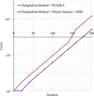
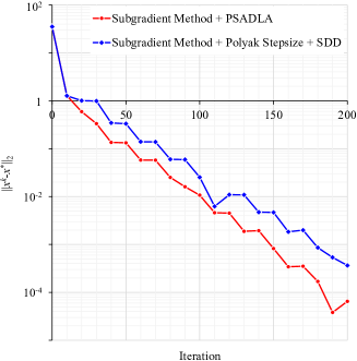
Figure 1: $L_{1}$ approximation problem: Comparison of subgradient methods with Polyak stepsizes and level adjustments through PSVD and SDD

When we extend the analysis to 200 iterations, the level value and solution obtained using the PSADLA method are roughly an order of magnitude closer to the true optimal values $f^{*}$ and $x^{*}$, respectively, compared to the results using the Polyak method with SDD-based level adjustment.

The problem is also solved by the Approximate Subgradient Method with PSADLA developed in Section 3. To obtain approximate subgradients, subgradients for a batch of 50 objective components are obtained at a time sequentially. The empirical evidence suggests that Condition 48 with $\varepsilon=10^{-10}$ is always satisfied. After calculating subgradients for all components once, the solution undergoes ten updates constituting one “outer” or “major iteration” (akin to a notion of an “epoch” in machine learning). The resulting level values are shown in Figure 2 (left), and the distance $\|x^{k}-x^{*}\|_{2}$ is shown in Figure 2 (right). The results obtained by Approximate Subradient + PSADLA (black) developed in Section 3 are benchmarked against those of Subradient + PSADLA (red) developed in Section 2. Notably, within the former, distances $\|x^{k}-x^{*}\|_{2}$ get progressively closer to 0: after 70 iterations, results are closer to 0 by one order of magnitude, after 120 iterations, results are closer by two orders of magnitude, and by iteration 180, result are three orders of magnitude closer.

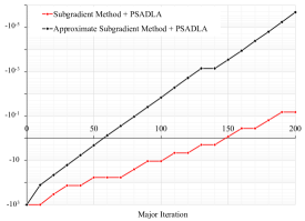
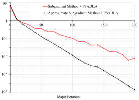
Figure 2: $L_{1}$ approximation problem: Comparison of subgradient and surrogate subgradient methods with PSADLA

4.2 Dual Problems of Generalized Assignment Problems

In this example, the dual problem of the generalized assignment problem [7] is optimized. The generalized assignment problem is to assign a set of jobs to a set of machines to minimize the total assignment cost $\sum_{i=1}^{I}\sum_{n=1}^{N}g_{i,n}y_{i,n}$, subject to $\sum_{n=1}^{N}y_{i,n}=1,\forall i=1,\ldots,I$ and $\sum_{i=1}^{I}c_{i,n}y_{i,n}\leq C_{n},\forall n=1,\ldots,N$, where $\{y_{i,n}\}$ are binary decision variables, $g_{i,n}$ is the cost of assigning job $i$ on machine $n$, $c_{i,n}$ is the time required to process job $i$ on machine $n$, and $C_{n}$ is the capacity of machine $n$. The dual problem to be optimized is

$$\underset{x\in\mathbb{R}^{n}}{\text{maximize}} f(x), x\geq 0,$$ subject to (94)

where $f(x)=\sup_{\left\{y_{i,n}\right\}\in\Omega_{1}}L(y,x)$ is the dual function with

$$L(y,x)=\sum_{i=1}^{I}\sum_{n=1}^{N}g_{i,n}y_{i,n}+\sum_{n=1}^{N}x_{n}\left(\sum_{i=1}^{I}c_{i,n}y_{i,n}-C_{n}\right)$$ (95)

being Lagrangian function and $\Omega_{1}=\left\{\left\{y_{i,n}\right\}\mid y_{i,n}\in\{0,1\},\sum_{n=1}^{N}y_{i,n}=1\right\}$. The dual function $f(\cdot)$ is a piece-wise linear non-smooth function. To calculate a subgradient of $f(\cdot)$ at a point $x^{k}$, $L(y,x^{k})$ is exactly optimized subject to $\Omega_{1}$. In previous sections, the minimization problem is considered.

Note: When solving maximization problems, the corresponding solution updating formula becomes $x^{k+1}=[x^{k}+s^{k}\cdot g^{k}]^{+}$, a level value $\bar{f}_{k}$ becomes an over-estimate of $f^{*}$, the stepsize becomes calculated as $s^{k}=\gamma\cdot\frac{\bar{f}_{k}-L\left(\tilde{y}^{k},x^{k}\right)}{\left\|g^{k}\right\|^{2}}$ and the Surrogate Optimality Condition (83) becomes $L\left(\tilde{y}^{k},x^{k}\right)<L\left(\tilde{y}^{k-1},x^{k}\right).$

Standard test instances from the OR library [1] are considered. The first problem instance is d201600 with 1600 jobs and 20 machines. The initial level value and solutions are chosen far from their optimal values to stress-test the method. Specifically, the initial level is set as 500,000, and the initial solution $x^{0}$ is randomly sampled from the uniform distribution U[0, 100]. The algorithm stops after 500 major iterations.

Comparison of Gaps. The level values $\bar{f}_{k}$ are upper bounds to $f^{*}$ whereas $f(x^{k})$ are lower bounds; the difference between $f(x^{k})$ and $\bar{f}_{k}$ – a gap – can be used to quantify the quality of $x^{k}$. In Figure 3 (left), the reduction of the gaps within subgradient methods (with PSADLA and SDD) is shown.

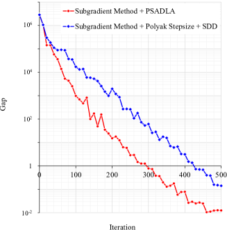
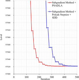
Figure 3: Reduction of gaps (left) and level values (right) for the dual problem (94) within subgradient methods (with PSADLA and SDD)

Comparison of Level Values. The level values are also shown in Figure 3 (right). With the PSADLA approach of this paper, the level value (shown in red) is adjusted fast. For comparison purposes, level adjustment through SDD [5] is also tested, and the results are shown in blue; the PSADLA approach leads to faster convergence.

Comparison of $f(x^{k})$ Values. The Simple Subgradient-Level Method of [10] is also tested for comparison. The function values versus iterations are shown in Figure 4, significantly lagging behind the two decision-based level-adjustment approaches.

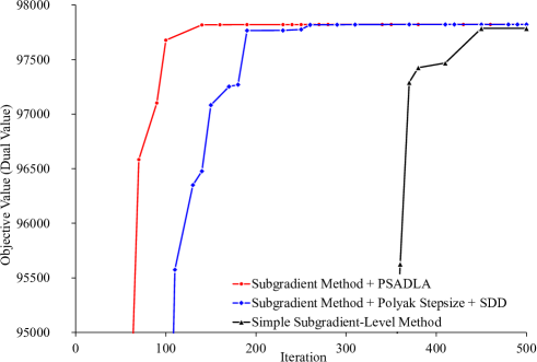
Figure 4: Optimizing the dual problem (94) of GAP d201600: Convergence of dual values within subgradient methods with PSADLA (this paper), SDD ([5]), and within the Simple Subgradient-Level Method ([10])

The hyperparameters of the simple subgradient level method $\delta^{0}$ and $B$ need to be fine-tuned. Performance of the method is tested by using a combination of the values $\delta^{0}\in\{5\times 10^{4},1\times 10^{5},5\times 10^{5},1\times 10^{6}\}$ and $B\in\{1,5,10,50,100\}$. The highest values of $f(x^{k})$ obtained across iterations before stopping under each choice of hyperparameters are listed in the second column of Table 1. The performance is significantly affected by the choice of the hyperparameters. The best value of 97790.55 is obtained for $\delta^{0}=1\times 10^{6},B=5$.

Table 1: Optimizing Generalized Assignment Problems: Comparison with the Simple Subgradient-Level (SL) Method

Method	$d201600$	$d401600$	$d801600$
Our (Initial level = $5\times 10^{5}$)	97,821.35	97,105.00	97,034.00
SL ($\delta^{0}=5\times 10^{4},B=1$)	26,706.02	72,668.02	30,200.96
SL ($\delta^{0}=5\times 10^{4},B=5$)	97,585.64	97,062.39	9,3525.12
SL ($\delta^{0}=5\times 10^{4},B=10$)	97,690.25	97,062.98	96,885.12
SL ($\delta^{0}=5\times 10^{4},B=50$)	97,018.37	96,850.18	96,855.04
SL ($\delta^{0}=5\times 10^{4},B=100$)	94,370.76	96,192.75	96,545.99
SL ($\delta^{0}=1\times 10^{5},B=1$)	49,828.70	80,999.68	33,745.26
SL ($\delta^{0}=1\times 10^{5},B=5$)	97,749.26	97,067.28	93,850.89
SL ($\delta^{0}=1\times 10^{5},B=10$)	97,772.69	97,048.22	96,875.47
SL ($\delta^{0}=1\times 10^{5},B=50$)	96,906.32	96,737.94	96,725.06
SL ($\delta^{0}=1\times 10^{5},B=100$)	94,705.43	96,135.46	96,654.81
SL ($\delta^{0}=5\times 10^{5},B=1$)	77,724.62	91,885.73	43,192.58
SL ($\delta^{0}=5\times 10^{5},B=5$)	97,773.52	$$97,080.50$$	94,788.83
SL ($\delta^{0}=5\times 10^{5},B=10$)	97,767.97	97,042.94	$$96,962.92$$
SL ($\delta^{0}=5\times 10^{5},B=50$)	97,108.43	96,948.04	96,638.00
SL ($\delta^{0}=5\times 10^{5},B=100$)	96,628.42	96,674.95	96,229.54
SL ($\delta^{0}=1\times 10^{6},B=1$)	82,047.64	92,414.48	41,396.42
SL ($\delta^{0}=1\times 10^{6},B=5$)	$$97,790.55$$	97,064.48	94,836.61
SL ($\delta^{0}=1\times 10^{6},B=10$)	97,760.81	97,041.48	96,915.84
SL ($\delta^{0}=1\times 10^{6},B=50$)	97,026.54	96,886.25	96,661.95
SL ($\delta^{0}=1\times 10^{6},B=100$)	96,118.86	96,686.40	96,547.11

The scalability of the method is demonstrated by considering larger instances. The results for both the 40-machine (d401600) and 80-machine (d801600) instances show a consistent level of accuracy, indicating good scalability: For d401600, the process is stopped at 1000 iterations, achieving a best function value of 97,104.99998 and a level value of 97,105.00007. For d801600, the process is stopped at 1500 iterations, achieving a best function value of 97,033.9998 and a level value of 97,034.0007. The method maintains a “razor-thin” accuracy in larger instances, showcasing its effectiveness in handling increased complexity.

In contrast, the Simple Subgradient-Level Method [10] exhibited high sensitivity to hyperparameter variations – the best results boxed in Table 1 correspond to different hyperparameter values.

4.3 Dual Problems of Job Assignment Problems with Transportation Time

In this example, a dual problem of another assignment problem is considered and the approximate subgradient of subsection 3.2.2 is tested. Before formulating the dual problem to be optimized, the assignment problem is first introduced briefly. If the $j^{th}$ operation of job $i$ is assigned to machine $n$, then $\{y_{i,j,n}\}$ equals 1. Otherwise, it is zero. Each operation needs to be assigned to a unique machine:

$$\sum_{n\in\Phi_{(i,j)}}y_{i,j,n}=1,\forall i=1,\ldots,I,j=1,\ldots,J_{i},$$ (96)

where $\Phi_{(i,j)}$ is the set of machines eligible to process the $j^{th}$ operation of job $i$. Following [9, 21], jobs need to go through a sequence of operations on multiple machines, and moving a job from one machine to another incurs transportation costs. The transportation cost for operation $(i,j)$, which is denoted as $z_{i,j}$ can be formulated as

$$t_{i,n_{1},n_{2}}\cdot\left(y_{i,j,n_{1}}+y_{i,j+1,n_{2}}-1\right)\leq z_{i,j},$$ (97)

$$\forall i=1,\ldots,I,j=1,\ldots,J_{i}-1,n_{1}\in\Phi_{(i,j)},n_{2}\in\Phi_{(i,j+1)},$$

where $t_{i,n_{1},n_{2}}$ denotes the transportation cost required to move job $i$ from machine $n_{1}$ to $n_{2}$. Each machine has a limited capacity, i.e.,

$$\sum_{(i,j)\in\Psi_{n}}c_{i,j,n}y_{i,j,n}\leq C_{n},\forall n=1,\ldots,N,$$ (98)

where $\Psi_{n}$ denotes the set of operations that can be processed by machine $n$, $c_{i,j,n}$ denotes the capacity required by machine $n$ to process ($i,j$), and $C_{n}$ denotes the capacity of machine $n$. The objective is to minimize assignment and transportation costs:

$$\min\sum_{i=1}^{I}\sum_{j=1}^{J_{i}}\sum_{n=1}^{N}g_{i,j,n}y_{i,j,n}+\sum_{i=1}^{I}\sum_{j=1}^{J_{i}-1}z_{i,j},$$ (99)

where $g_{i,j,n}$ is the cost of processing ($i,j$) on machine $n$. After relaxing the capacity constraints (98) by using Lagrangian multipliers $x\in\mathbb{R}^{n}$, the relaxed problem can be written as

$$\underset{y,z}{\text{minimize}}\quad L(y,z,x),\quad\text{subject to}\quad\eqref{GAP_withtransportation_assignmentconstraints},\eqref{GAP_withtransportation_transcost},$$ (100)

with

$$L(y,z,x)=\sum_{i=1}^{I}\sum_{j=1}^{J_{i}}\sum_{n=1}^{N}g_{i,j,n}y_{i,j,n}+\sum_{i=1}^{I}\sum_{j=1}^{J_{i}-1}z_{i,j}+\sum_{n=1}^{N}x_{n}\left(\sum_{(i,j)\in\Psi_{n}}c_{i,j,n}y_{i,j,n}-C_{n}\right).$$ (101)

The dual problem then becomes

$$\underset{x}{\text{maximize}} q(x)\equiv\inf_{\left\{y_{i,j,n},z_{i,j}\right\}\in\Omega_{2}}L(y,z,x),\quad\text{subject to} x\geq 0,$$ (102)

where $\Omega_{2}=\left\{\left\{y_{i,j,n},z_{i,j}\right\}\mid y_{i,j,n}\in\{0,1\},z_{i,j}\geq 0,s.t.\eqref{GAP_withtransportation_assignmentconstraints},\eqref{GAP_withtransportation_transcost}\right\}$. The instance data with 40 machines and 40 jobs is generated randomly, and each job has 10 operations. For simplicity, we assume that each machine is eligible to process all operations. The assignment costs $\{g_{i,j,n}\}$, the capacities $\{c_{i,j,n}\}$ required by operations, the machine capacities $\{c_{n}\}$, and transportation costs $\{t_{i,n_{1},n_{2}}\}$ are sampled from uniform distributions. Since the relaxed problem is an ILP problem, Branch-and-Cut implemented by IBM CPLEX is used to solve it to calculate subgradients and approximate subgradients.

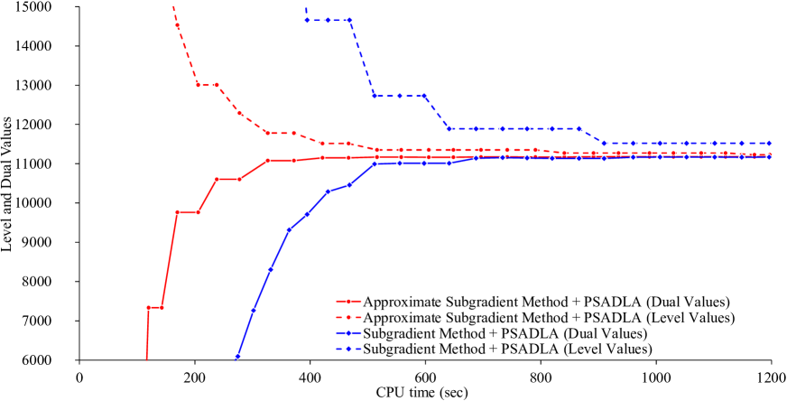
Figure 5: Optimizing the dual problem (102) by subgradient methods and surrogate subgradient methods with PSADLA

The Lagrangian function within (100) is additive in terms of jobs. Every 10 jobs are grouped to form a subproblem, which is solved to satisfy the surrogate optimality condition (83). The initial level value is set as 20,000 – much larger than $f^{\star}$. The initial decision variable $x^{0}$ is sampled from $U[0,100]$. The stopping criterion is 1200 sec., which includes initialization, subgradient, and solution calculations, as well as level adjustment times. The results are shown in Figure 5. Before stopping, subproblem solutions are updated 305 times requiring 3.82 sec. to obtain approximate subgradients, on average. Because of the linearity of the PSVD problem (51), checking its feasibility requires only 0.06 sec. on average. High-quality solutions are thus obtained in a computationally efficient manner. For comparison, the subgradient approach with PSADLA is also tested, and the results are also shown in Figure. 5. Since the relaxed problem (100) needs to be optimally solved to obtain a subgradient, before stopping, the solution is only updated 78 times. As a result, the subgradient approach is slower than the approximate subgradient approach.

5 Conclusions

In this paper, a Polyak Stepsize with Accelerated Decision-guided Level Adjustment (PSADLA) is developed for subgradient optimization. Convergence is rigorously established, and the results are extended to approximate subgradients, leading to significant CPU time savings. Testing results across various convex problems with distinct characteristics show that the level value is efficiently adjusted, leading to fast convergence. The approach holds promise for discrete programs and machine learning applications.

References

- [1] J. E. Beasley. Or-library: distributing test problems by electronic mail. Journal of the operational research society, 41(11):1069–1072, 1990.
- [2] D. P. Bertsekas. Nonlinear programming 3rd edition. Journal of the Operational Research Society, 48(3):334–334, 1997.
- [3] S. P. Boyd and L. Vandenberghe. Convex optimization. Cambridge university press, 2004.
- [4] M. A. Bragin, P. B. Luh, J. H. Yan, N. Yu, and G. A. Stern. Convergence of the surrogate lagrangian relaxation method. Journal of Optimization Theory and Applications, 164(1):173–201, 2015.
- [5] M. A. Bragin and E. L. Tucker. Surrogate “level-based” lagrangian relaxation for mixed-integer linear programming. Scientific Reports, 12(1):22417, 2022.
- [6] U. Brannlund. On relaxation methods for nonsmooth convex optimization. 1995.
- [7] D. G. Cattrysse and L. N. Van Wassenhove. A survey of algorithms for the generalized assignment problem. European journal of operational research, 60(3):260–272, 1992.
- [8] I. I. Cplex. Ibm ilog cplex optimization studio cplex user’s manual. Armonk, NY, USA: IBM, 2011.
- [9] L. Deroussi, M. Gourgand, and N. Tchernev. A simple metaheuristic approach to the simultaneous scheduling of machines and automated guided vehicles. International Journal of Production Research, 46(8):2143–2164, 2008.
- [10] J.-L. Goffin and K. C. Kiwiel. Convergence of a simple subgradient level method. Mathematical Programming, 85(1):207–211, 1999.
- [11] E. Lim and P. W. Glynn. Consistency of multidimensional convex regression. Operations Research, 60(1):196–208, 2012.
- [12] N. Loizou, S. Vaswani, I. H. Laradji, and S. Lacoste-Julien. Stochastic polyak step-size for sgd: An adaptive learning rate for fast convergence. In International Conference on Artificial Intelligence and Statistics, pages 1306–1314. PMLR, 2021.
- [13] K. Mao, Q.-K. Pan, T. Chai, and P. B. Luh. An effective subgradient method for scheduling a steelmaking-continuous casting process. IEEE Transactions on Automation Science and Engineering, 12(3):1140–1152, 2014.
- [14] A. Nedic and D. P. Bertsekas. Incremental subgradient methods for nondifferentiable optimization. SIAM Journal on Optimization, 12(1):109–138, 2001.
- [15] A. Orvieto, S. Lacoste-Julien, and N. Loizou. Dynamics of sgd with stochastic polyak stepsizes: Truly adaptive variants and convergence to exact solution. Advances in Neural Information Processing Systems, 35:26943–26954, 2022.
- [16] M. R. Osborne, B. Presnell, and B. A. Turlach. On the lasso and its dual. Journal of Computational and Graphical statistics, 9(2):319–337, 2000.
- [17] D. A. Pisner and D. M. Schnyer. Support vector machine. In Machine learning, pages 101–121. Elsevier, 2020.
- [18] B. T. Polyak. Minimization of unsmooth functionals. USSR Computational Mathematics and Mathematical Physics, 9(3):14–29, 1969.
- [19] B. T. Polyak. Subgradient methods: a survey of soviet research. Nonsmooth optimization, 3:5–29, 1978.
- [20] T. Sun, Q. Zhao, and P. Luh. On the surrogate gradient algorithm for lagrangian relaxation. Journal of optimization theory and applications, 133(3):413–416, 2007.
- [21] Q. Zhang, H. Manier, and M.-A. Manier. A genetic algorithm with tabu search procedure for flexible job shop scheduling with transportation constraints and bounded processing times. Computers & Operations Research, 39(7):1713–1723, 2012.
- [22] X. Zhao, P. B. Luh, and J. Wang. Surrogate gradient algorithm for lagrangian relaxation. Journal of optimization Theory and Applications, 100(3):699–712, 1999.