Algorithmic Persuasion Through Simulation

Abstract

We study a Bayesian persuasion problem where a sender wants to persuade a receiver to take a binary action, such as purchasing a product. The sender is informed about the (binary) state of the world, such as whether the quality of the product is high or low, but only has limited information about the receiver’s beliefs and utilities. Motivated by customer surveys, user studies, and recent advances in generative AI, we allow the sender to learn more about the receiver by querying an oracle that simulates the receiver’s behavior. After a fixed number of queries, the sender commits to a messaging policy and the receiver takes the action that maximizes her expected utility given the message she receives. We characterize the sender’s optimal messaging policy given any distribution over receiver types. We then design a polynomial-time querying algorithm that optimizes the sender’s expected utility in this Bayesian persuasion game. We also consider approximate oracles, more general query structures, and costly queries.

1 Introduction

Information design is a canonical branch of theoretical economics that analyzes how provision of information by an informed designer influences the strategic behavior of agents in a game. We initiate the study of information design with oracle access. This oracle is endowed with information about the agents and can be queried by the designer in order to refine her beliefs and thus improve her decision of what information to convey to the agents.

We focus on Bayesian persuasion [Kamenica and Gentzkow, 2011, Kamenica, 2019], a paradigmatic setting in information design. Bayesian persuasion is an information design game between two players: an informed sender (i.e. designer), who observes the state of the world, and an uninformed receiver (i.e. agent), who does not see the state but takes an action. The payoffs of both players depend on both the world’s state and the receiver’s action. The game proceeds as follows: The sender commits to a messaging policy, i.e. a mechanism for revealing information to the receiver about the state of the world, before the state is realized. Once the state is realized, the sender sends a message to the receiver according to their messaging policy. Upon receiving the message, the receiver updates her belief about the state of the world, and takes an action.

The sender’s payoff-maximizing messaging policy often depends on information about the receiver; for example, the receiver’s utility function or her belief about the state of the world. The standard setting assumes the sender has full information about the receiver, but this may not always be the case. The line of work on robust Bayesian persuasion (e.g. Dworczak and Pavan [2022], Parakhonyak and Sobolev [2022], Hu and Weng [2021]) and Bayesian persuasion with an informed receiver (e.g. Kolotilin et al. [2017]) takes the other extreme, assuming the sender must determine the messaging policy with limited information about the receiver. Such message policies are applicable in a wider range of settings when compared to methods which require full information about the receiver, but extract less utility for the sender.

Our model of Bayesian persuasion with agent-informed oracle access posits that many settings lie between these extremes. The sender may acquire additional information about the receiver through external sources. Our main focus is on oracles that simulate the receiver’s action in different settings. The sender may be able to acquire this type of information through one of the following processes:

1. Receiver simulation using AI. Given sufficient data about the receiver, the sender could attempt to predict the receiver’s action using machine learning. Suppose the sender is an online marketplace who wants to bring a new product to market and the buyer is a marketplace user. While the sender may initially be unsure about how the new product will be received, they may be able to use a user’s purchase history on the platform to predict how positively the user would respond to a sales pitch for the new product. Recent research demonstrates that generative AI can also help obtain insights about how humans may behave in real-world strategic scenarios (e.g. Horton [2023], Fish et al. [2023]). Notably, in experiments, this technology often makes consumer choices that track with those of humans. They exhibit downward-sloping demand curves, diminishing marginal utility of wealth, and state dependence, and further match the stated willingness-to-pay of consumers in a recent market survey [Brand et al., 2023]. They even exhibit (sometimes non-strategic) behaviors consistent with particular demographics given appropriate framing, such as libertarians in the context of pricing [Horton, 2023] or women in the context of ultimatum games [Aher et al., 2023]. Finally, if the receiver is itself an AI agent or relies heavily on one, e.g., in online markets, ad auctions, or gaming, it may be possible to simulate them directly through access to (or knowledge of) the AI agent. In each of these cases, the sender must incur some cost to query the oracle.

2. Simulation as a metaphor for exploration. An agent-informed oracle can also be a metaphor for market research that the sender performs before interacting with the receiver. For example, a startup may test out its funding pitch on smaller venture capital firms before trying to persuade a larger firm to fund their business. A company may run a customer focus group before bringing a new product or service to market, or experiment on a fraction of users in online services (e.g. Kohavi et al. [2009], Kohavi and Longbotham [2017]). Again, the “queries” in these settings are expensive; a startup may have a limited number of venture capital firms that it can pitch to, and a company may be limited in the number of customers/users it can engage in advance without disrupting overall sales.

In each of these scenarios, an agent-informed oracle is potentially very useful to the sender but also costly to invoke. It is therefore important to understand how to employ them effectively and efficiently, and how to quantify their benefit. A sender with a generative AI query budget must understand which potential query (or queries) will produce the greatest benefit; a seller debating whether to commission more rounds of market research should calculate whether the expected benefits outweigh the costs. Complicating the situation, the space of potential queries can be enormous and the information provided by one query can complement revelations from previous queries. It is therefore crucial to understand the algorithmic problem of computing optimal (or near-optimal) adaptive query sequences for the sender.

We focus on a Bayesian persuasion setting in which both the state and action set are binary. We further assume the sender’s utility is state-independent. (Both assumptions are common special cases in economics, see, e.g., Parakhonyak and Sobolev [2022], Kosterina [2022], Hu and Weng [2021], Kolotilin et al. [2017].) One motivating example of this setting is the interaction between a seller of a product (the sender) and a potential buyer (the receiver). The state of the world is the quality of the product (e.g., high/low quality) and the message corresponds to the sales pitch presented to the buyer. The seller would always like to sell, but the buyer only wants to buy if the product is of sufficiently high quality. A buyer-informed oracle may help the seller optimize her sales pitch. In Bayesian persuasion, the seller must commit to this sales pitch before observing the product quality; this ability to commit may arise from, e.g. legal regulations or the seller’s desire to protect her reputation.

As in the traditional setting, we assume the sender has full knowledge of the utility structure. However, the receiver has private information about the state, yielding an information asymmetry advantaging the receiver. Specifically, we assume the receiver has a private signal correlated with the state. The sender knows the joint distribution of signal and state but does not know the specific signal that the receiver obtained. This might be the case if, for instance, the receiver has previously heard about the product from external sources.

The sender can query the oracle to gain additional information about the receiver’s belief. We focus on a particular type of oracle which we call a simulation oracle. Such an oracle inputs a messaging policy and a particular message realization, and outputs the action that would have been chosen by the receiver (given her belief) upon seeing this policy and this message. We assume the sender is subject to a query budget, i.e., she can make only a fixed number of queries to the oracle.

The timing of our game is as follows: the sender (i) queries the oracle according to some querying policy and (ii) computes a messaging policy using the information gained from the oracle; then (iii) the state is revealed to the sender and the message is communicated to the receiver, and (iv) the receiver chooses an action.

From an algorithmic perspective, our goal is to optimize the sender’s Bayesian-expected utility in the perfect Bayesian equilibrium of the game. Our technical analysis is mainly concerned with the problem of computing an optimal querying policy for step (i). In order to do so, we first characterize the sender’s optimal messaging policy from (ii) given an arbitrary set of beliefs about the receiver’s type induced by the oracle queries. Indeed, we show that receiver types can be totally ordered by a measure of how easily they can be convinced to take an action. Given any set of information revealed from oracle queries, we make use of a well-known encoding of the sender’s message optimization problem as a linear program; the geometry of its constraints under our total ordering of receivers implies that the sender’s optimal messaging policy is always supported on at most two messages, each corresponding to a threshold receiver type.

Given our characterization of optimal messaging given a set of queries, we show that an optimal querying policy can be found via dynamic programming in time polynomial in the size of the type space. Our algorithm takes advantage of a natural geometric interpretation of oracle queries induced by the binary setting. Namely, since receiver beliefs are totally ordered by the intensity of the message required to convince them to take an action, an oracle query corresponds to a threshold on the type space. We leverage this ordering to compute an optimal querying policy via dynamic programming. We also bound the sensitivity of the sender’s optimal querying policy to noise in the distribution over receiver beliefs, showing that performance degrades gracefully with small perturbations. This enables us to discretize the space of receiver types, resulting in an $\epsilon$-approximately optimal querying policy that can be constructed in time polynomial in $1/\epsilon$.

1.1 Related Work

Bayesian Persuasion (BP) was introduced by Kamenica and Gentzkow [2011], and has been extensively studied since then, see Kamenica [2019] for a recent survey. The most relevant direction is robust BP, which aims to relax the assumptions on the information the sender has about the receiver [Dworczak and Pavan, 2022, Hu and Weng, 2021, Parakhonyak and Sobolev, 2022, Kosterina, 2022, Zu et al., 2021]. This line of work typically focuses on characterizing the “minimax” messaging policy (i.e., one that is worst-case optimal over the sender’s uncertainty), while our focus is on using oracle queries to help the sender overcome her uncertainty. Our work is also related to online BP [Castiglioni et al., 2020, 2021, Bernasconi et al., 2023, Zu et al., 2021], where the sender interacts with a sequence of receivers. In prior work on this variant, the sequence of receivers is adversarially chosen, and the sender minimizes regret. Our model (with a simulation oracle) can be interpreted as a “pure exploration” variant of online BP. Indeed, all $K$ oracle calls simulate the same “real” receiver, and are provided for free.

Large Language Models (LLMs) in Economics. A rapidly growing line of work at the intersection of computer science and economics explores the use of LLMs in various economic contexts. Aside from LLM-simulated economic agents discussed in Section 1, this line of work studies LLM-simulated (human-driven) experiments in behavioral economics [Horton, 2023], LLM-generated persuasive messages [Matz et al., 2023], LLM-simulated human day-to-day behavior [Park et al., 2023], LLM-predicted opinions for nationally representative surveys [Kim and Lee, 2023], and auction mechanisms to combine LLM outputs [Duetting et al., 2023]. A growing body of work uses LLMs to make strategic decisions in various scenarios [Lorè and Heydari, 2023, Akata et al., 2023, Brookins and DeBacker, 2023, Chen et al., 2023, Guo, 2023, Tsuchihashi, 2023]. Finally, simultaneous work [Fish et al., 2023] adopts a conceptually similar approach with LLM-based oracles, focusing on social choice. Their framework combines social choice theory with LLMs’ ability to generate unforeseen alternatives and extrapolate preferences.

Simulation in Games. Kovarik et al. [2023] study a normal-form game setting in which one player can simulate the behavior of the other. In contrast, we study simulation in Bayesian persuasion games, which are a type of Stackelberg game [Von Stackelberg, 1934, Conitzer and Sandholm, 2006]. There is a line of work on learning the optimal strategy to commit to in Stackelberg games from query access [Letchford et al., 2009, Peng et al., 2019, Blum et al., 2014, Balcan et al., 2015]. However, the type of Stackelberg game considered in this line of work is different from ours. In this setting, the leader (the leader is analogous to the sender in our setting) specifies a mixed strategy over a finite set of actions. In contrast, in our setting the sender commits to a messaging policy which specifies a probability distribution over actions for every possible state realization.

2 Model

We study a Bayesian persuasion game with an informed receiver. There is a binary state of the world $\omega\in\Omega=\{0,1\}$. The receiver has a private signal about the state $s\in\mathcal{S}$. We assume $\mathcal{S}$ is finite and write $T=|\mathcal{S}|$. The state and signal are drawn from a joint distribution $F$. Given $s\in\mathcal{S}$, we write $F|_{s}$ for the marginal distribution over $\omega$ given $s$. The receiver can take one of two actions $a\in\mathcal{A}=\{0,1\}$. Sender and receiver utilities are given by utility functions $u_{S}:\Omega\times\mathcal{A}\rightarrow\mathbb{R}$ and $u_{R}:\Omega\times\mathcal{A}\rightarrow\mathbb{R}$ respectively. We assume the sender’s utility is state-independent and positive only if the receiver takes the action $a=1$, i.e., $u_{S}(\omega,a)=a$. The receiver’s utility depends on whether the action matches the state, i.e., $u_{R}(\omega,a)=\mathbf{1}(a=\omega)$. The joint distribution $F$ as well as the utility functions $u_{S}$ and $u_{R}$ are known to both the sender and the receiver; the signal $s$ is known only to the receiver. We refer to this setting as Binary Bayesian Persuasion.

The sender commits to a messaging policy which maps states to messages.

Definition 2.1 (Messaging Policy).

The sender’s messaging policy $\sigma:\Omega\rightarrow\mathcal{M}$ is a (randomized) mapping from states to messages $m\in\mathcal{M}$.

We will sometimes write $\sigma(m|\omega)$ to denote $\Pr[\sigma(\omega)=m]$ and $m\sim\sigma(\omega)$ to denote a message sampled from $\sigma$ when the state is $\omega\in\Omega$.

We depart from prior formulations of this problem in our assumption that the sender has access to a simulation oracle. This oracle simulates the receiver’s optimal actions and thus yields information about the receiver’s signal, $s$, which helps the sender improve its messaging policy.

Definition 2.2 (Simulation Oracle).

A simulation oracle inputs a query $q\in\mathcal{Q}$ consisting of a tuple $(\sigma_{q},m_{q})$, where $\sigma_{q}$ is a messaging policy and $m_{q}\in\mathcal{A}$ is a message. The oracle returns the receiver’s best-response given the joint distribution $F$ and private signal $s$, i.e., it returns $a_{q}$ where:

$$a_{q}=\arg\max_{a\in\mathcal{A}}\mathbb{E}_{\omega}[u_{R}(\omega,a)|m_{q},s].$$

We assume the sender can make up to $K$ queries and can do so adaptively. That is, the sender can sequentially make queries, choosing each next query based on the responses to the previous queries. Formally, a history is a finite (possibly empty) sequence of query-action pairs. We write $\mathcal{H}$ for the set of all histories. We denote the sender’s querying policy by the function $\pi\colon\mathcal{H}\to\mathcal{Q}$ that maps a sequence of past queries and responses to a next query. We will also abuse notation and write $\pi(s)$ to denote the history generated by the application of $\pi$ until its termination, where $s\in\mathcal{S}$ is the receiver’s signal.

Protocol: Bayesian Persuasion with Oracle Queries 1. the sender uses querying policy $\pi$ to query the simulation oracle up to $K$ times, resulting in query history $H$; 2. the sender commits to a messaging policy $\sigma_{H}$, which is visible to the receiver; 3. the state $\omega$ is revealed privately to the sender; 4. the message $m\sim\sigma_{H}(\omega)$ is sent to the receiver; 5. the receiver chooses an action $a=a(m)\in\mathcal{A}$.

Figure 1: Summary of our setting.

The timing of the game is summarized in Figure 1. We study perfect Bayesian equilibria (PBE) of this game. In our game, a strategy for the sender is a querying policy $\pi$, plus a messaging policy rule $\sigma$ that maps potential query histories to messaging policies (where we write $\sigma_{H}$ for the messaging policy corresponding to query history $H$). A strategy for the receiver is an action rule $a\colon\mathcal{M}\times\mathcal{S}\to\mathcal{A}$ mapping a message and a signal to an action.

Definition 2.3 (Perfect Bayesian Equilibrium).

A profile of strategies $(\pi^{*},\sigma^{*},a^{*})$, together with a belief rule $B_{S}\colon\mathcal{H}\to\Delta(\mathcal{S})$ for the sender mapping query histories to distributions over receiver signals, plus a belief rule $B_{R}\colon\mathcal{M}\times\mathcal{S}\to\Delta(\Omega)$ for the receiver mapping messages and signals to distributions over the state of the world, is a perfect Bayesian equilibrium if:

1. For each $m\in\mathcal{M}$ and $s\in\mathcal{S}$, action $a^{*}(m,s)$ maximizes the receiver’s expected utility given belief $B_{R}(m,s)$:

   $$a^{*}(m)\in\arg\max_{a}\{\mathbb{E}_{\omega\sim B_{R}(m)}[u_{R}(\omega,a)]\}$$

2. Belief $B_{R}(m,s)$ is the correct posterior distribution over $\omega$ given $s$, $\sigma^{*}_{H}$, and the fact that $\sigma^{*}_{H}(\omega)=m$.

3. For each $H\in\mathcal{H}$, messaging policy $\sigma^{*}_{H}$ maximizes the sender’s expected utility given belief $B_{S}(H)$:

   $$\sigma^{*}_{H}\in\arg\max_{\sigma}\{\mathbb{E}_{s\sim B_{S}(H),\omega\sim F|_{s}}[u_{S}(\omega,a^{*}(\sigma(\omega),s))]$$

4. Belief $B_{S}(H)$ is a correct posterior distribution over $s$, given $\pi^{*}$ and the fact that $\pi^{*}$ generates history $H$.

5. Sender’s querying policy $\pi^{*}$ maximizes the sender’s expected utility given $\sigma^{*}$ and $a^{*}$:

   $$\pi^{*}\in\arg\max_{\pi}\{\mathbb{E}_{(\omega,s)\sim F,H\sim\pi}[u_{S}(\omega,a^{*}(\sigma^{*}_{H}(\omega),s))]\}$$

A few notes are in order. We emphasize that the state $\omega$ is revealed to the sender only after the messaging policy $\sigma_{H}$ is announced, so the query history has no dependency on $\omega$ after conditioning on $s$. In particular, this means that since the messaging policy $\sigma^{*}_{H}$ is observable by the receiver, the query history $H$ has no further bearing on the receiver’s beliefs, utility, or choice of action.

We also note that optimality of the querying policy $\pi^{*}$ implies that, given any partial history $H$ of fewer than $K$ queries, the subsequently chosen query $\pi^{*}(H)$ must also be utility-optimizing for the sender given the posterior over $s$ induced by $H$. And while we do not impose the restriction explicitly, we note that since the generation of histories $H$ is mechanical given the choice of $\pi^{*}$ and the realization of $s$, any history $H$ that is inconsistent with any realization of $s$ will have probability $0$ of being observed, even off the equilibrium path of play.

Finally, we note that we assumed the receiver has a private signal correlated with the state and thus knows something about the state that the sender does not at the beginning of the game. This (rather standard) setting is sometimes motivated by scenarios where the receiver might have access to news that the sender does not have access to when designing her messaging policy. It can be interesting to consider what happens if the receiver has “fake” news but acts as if her news is true. One way to model this is to assume that two pairs of world state and signal are drawn independently from $F$, say $(\omega,s),(\omega^{\prime},s^{\prime})\sim F$, where $\omega$ is the true state but the receiver observes signal $s^{\prime}$ and (incorrectly) infers that $\omega$ is distributed as $F|_{s^{\prime}}$. All of our results carry through to this setting with minor modifications to the algorithms.

3 Preliminaries

We begin with structural results which showcase intuition and will be useful later. We first show that any messaging policy is outcome-equivalent to one with just $T+1$ messages (recall that $T=|\mathcal{S}|$). We then use the underlying arguments of this proposition to derive a useful geometric property of simulation queries. Namely, we argue any simulation query is equivalent to a threshold that separates receivers into those whose belief in state $\omega=1$ is greater than a threshold $p\in[0,1]$ and those for whom it is less than $p$.

3.1 Optimal Persuasion Under Uncertainty

Our binary setting exhibits a particularly clean structure. In particular, as the action space is binary, for any messaging policy and any message sent according to that policy, the receiver beliefs are partitioned into two sets: those that induce action $a=1$ in response to the message and those that induce action $a=0$. Furthermore, since the state is binary, the heterogenity among possible receiver beliefs is single-dimensional and totally-ordered by the weight the belief places on a high state $\omega=1$. Therefore, the partition of beliefs induced by a message can be represented by a single threshold: beliefs higher than the threshold induce the action $a=1$ and those lower induce action $a=0$. These observations imply that the sender’s optimal messaging policy has size $T+1$.

To formalize this, note first that each signal $s\in\mathcal{S}$ induces a distribution $F|_{s}$ over $\Omega=\{0,1\}$, which can be described by a probability $p\in[0,1]$ that $\omega=1$. We can therefore equivalently describe each receiver’s private information as a (prior) belief $p\in[0,1]$, rather than a signal $s\in\mathcal{S}$. We will write $\mathcal{T}\subset[0,1]$ for the set of probabilities induced by signals in $\mathcal{S}$, which we can assume without loss of generality are distinct so that $T=|\mathcal{T}|$. We refer to $\mathcal{T}$ as the set of receiver beliefs, which we denote $\mathcal{T}=\{p_{1},p_{2},\dotsc,p_{T}\}$ where $p_{1}>p_{2}>\dotsc>p_{T}$, and write $\mathcal{P}(p_{i})$ for the probability (over the realization of signal $s$) that the receiver’s belief is $p_{i}$.

We say two messaging policies $\sigma$ and $\sigma^{\prime}$ are outcome equivalent if for all $\omega$, $m\in\sigma(\omega)$, $m^{\prime}\in\sigma^{\prime}(\omega)$ and receiver prior $p$, the receiver-optimal action $a$ upon seeing $m$ equals the receiver-optimal action $a^{\prime}$ upon seeing $m^{\prime}$. The following “revelation principle” is well-known in the literature on persuasion with multiple receivers; we prove it here for completeness.

Proposition 3.1.

In Binary BP, for any messaging policy $\sigma$, there is an outcome-equivalent policy $\sigma^{\prime}$ with just $M=T+1$. Moreover, these messages can be written as $\{m_{0},m_{1},\dotsc,m_{T}\}$, where a receiver with prior $p_{i}$ will take action $a=1$ upon receiving message $m_{j}$ if and only if $j\geq i$.

Proof.

A receiver with prior $p$ takes action $a=1$ after seeing message $m$ if and only if $p\geq\frac{\sigma(m|0)}{\sigma(m|1)+\sigma(m|0)}$. Therefore if a receiver with prior $p$ takes action $1$ after seeing a message $m$, any receiver with belief $p^{\prime}\geq p$ will also take action $a=1$. There are therefore at most $T+1$ distinct subsets of receiver beliefs that are induced to take action $a=1$ on any message $m$ of signaling policy $\sigma$, each corresponding to a minimal belief $p_{i}\in\mathcal{T}$ that takes the action (plus one more to denote no receiver taking the action).

Let $\sigma^{\prime}$ be the messaging policy with messages $m_{0},m_{1},\dotsc,m_{T}$, such that $\sigma^{\prime}(\omega)=m_{i}$ whenever $\sigma(\omega)$ would induce receivers with beliefs $\{p_{1},\dotsc,p_{i}\}$ to act (or $m_{0}$ if it induces no receiver to act). Then $\sigma$ and $\sigma^{\prime}$ are outcome equivalent by construction, and $\sigma^{\prime}$ has the required structure of $T+1$ messages. ∎

We note that $T+1$ messages may be necessary. For example, suppose there are two equally-likely receiver beliefs, $\{0.25,0.75\}$. In this case, a messaging policy with message space $\mathcal{M}=\{m_{0},m_{1},m_{2}\}$ that uniformly randomizes between messages $m_{0}$ and $m_{1}$ when $\omega=0$, and uniformly randomizes between messages $m_{1}$ and $m_{2}$ when $\omega=1$, induces unique behaviors on each message. Indeed, any receiver that receives message $m_{0}$ can infer that $\omega=0$ so they choose action $a=0$, and any receiver that receives message $m_{2}$ can infer that $\omega=1$ so they choose action $a=1$. However, upon receiving message $m_{1}$, an agent with belief $p_{i}$ will have posterior belief $p_{i}$ as well, so an agent of type $p_{1}=0.75$ would take action $a=1$ upon receiving message $m_{1}$, whereas an agent of type $p_{2}=0.25$ would not.

In Section 4.1 we show that there always exists a sender-optimal messaging policy that uses just $2$ messages. Nevertheless, we describe the structure of all (possibly suboptimal) messaging policies as it will be useful both as a stepping-stone toward that optimality characterization, and as a way to describe the geometry of simulation queries, which we explore next.

3.2 The Geometry of Simulation Queries

Another implication of the argument in Proposition 3.1 is that in Binary BP, there is a one-to-one correspondence between simulation queries and thresholds in $(0,1)$.

Proposition 3.2.

Given a simulation query $q=(\sigma,m)$ in Binary BP, the response $a_{q}$ is equal to $1$ if and only if the belief $p=Pr[\omega=1|s]$ of the receiver conditional on the private signal $s$ satisfies $p\geq\theta_{q}$, where

$$\theta_{q}=\frac{\sigma(m|\omega=1)}{\sigma(m|\omega=1)+\sigma(m|\omega=0)}.$$

This result implies that in Binary BP, there always exists a simulation query $q$ that can distinguish between any two receiver beliefs $p_{i}$, $p_{j}$ such that $p_{i}\neq p_{j}$. Furthermore, any simulation query implies a partition on beliefs defined by a threshold. We will use this in Section 4 to argue that the optimal querying policy of the sender can be characterized as choosing a set of thresholds.

4 Equilibrium Computation

In this section, we develop an algorithm that computes a sender-optimal equilibrium in time polynomial in the number of signals $T$. Fixing the actions of the sender, the receiver’s best response is simply a Bayesian update and hence computable in constant time. Fixing the querying policy, and so the posterior beliefs of the sender, we note using fairly standard techniques that the sender’s optimal message policy can be computed in quadratic time in Section 4.1. Thus the main challenge, discussed in Section 4.2, is computing the querying policy.

4.1 Optimal Messaging Policy

We first characterize the sender’s optimal messaging policy whenever she has uncertainty about the receiver’s belief. The optimal messaging policy has at most two messages, with the following interpretation. First, there is a message $m*$ with a threshold receiver belief $p^{*}$ such that a receiver with that belief is indifferent between action and inaction. All receivers with a posterior belief $p:=Pr[\omega=1|s]$ such that $p\geq p^{*}$ should take action $a=1$ upon receiving message $m^{*}$, and all those for which $p<p^{*}$ should take action $a=0$. There is at most one other message, and there are two cases for the behavior it induces: it either indicates that all receivers should take action $a=1$, or that no receivers should take action $a=1$.

Proposition 4.1.

[Optimal Messaging Policy] In Binary BP, for a given set of receiver beliefs $p_{L}>p_{L+1}>\dotsc>p_{H}$, the sender’s optimal messaging policy can be computed in time $\mathcal{O}((T^{\prime})^{2})$. The optimal policy is described by an index $i^{*}$ where

$$i^{*}:=\arg\max_{i^{\prime}\in[L,H]}\;\left\{\min\left\{1,\frac{1-p_{i^{\prime}}}{p_{i^{\prime}}}\right\}\sum_{i=L}^{i^{\prime}}\mathcal{P}(p_{i})\cdot\left(p_{i}+(1-p_{i})\cdot\frac{p_{i^{\prime}}}{1-p_{i^{\prime}}}\right)\right\}.$$

If $p_{i^{*}}\leq 1/2$, the optimal policy is given by $\sigma(m_{i^{*}}|1)=1$, $\sigma(m_{i^{*}}|0)=\frac{p_{i^{*}}}{1-p_{i^{*}}}$, and $\sigma(m_{0}|0)=1-\frac{p_{i^{*}}}{1-p_{i^{*}}}$; if $p_{i^{*}}>1/2$, the optimal policy is given by $\sigma(m_{i^{*}}|0)=1$, $\sigma(m_{i^{*}}|1)=\frac{1-p_{i^{*}}}{p_{i^{*}}}$, and $\sigma(m_{H}|1)=1-\frac{1-p_{i^{*}}}{p_{i^{*}}}$.

Proof.

By Proposition 3.2, it suffices to consider policies with messages $m_{0},m_{L},m_{L+1},\dotsc,m_{H}$, such that a receiver of belief $p_{i}$ chooses action $a=1$ on message $m_{j}$ if and only if $i\leq j$. We claim that the sender’s optimization can therefore be written as

$$\max_{\sigma}\;\sum_{i=L}^{H}\mathcal{P}(p_{i})\cdot\sum_{j=i}^{H}p_{i}\cdot\sigma(m_{j}|1) +(1-p_{i})\cdot\sigma(m_{j}|0)$$

$$\text{s.t. }\forall i\in[L,H],\;\;\sigma(m_{i}|0) \leq\frac{p_{i}}{1-p_{i}}\cdot\sigma(m_{i}|1)\quad\text{(IC)}$$

$$\sum_{i=L}^{H}\sigma(m_{i}|1) \leq 1$$

$$\sum_{i=L}^{H}\sigma(m_{i}|0) \leq 1.$$

To see why, note that the objective iterates over all possible realizations of receiver belief $p_{i}$, and for each one we sum over all messages $m_{j}$ that would induce a receiver of that type to take action $1$. The probability of receiving message $m_{j}$, given that the receiver’s belief is $p_{i}$, is then precisely $p_{i}\cdot\sigma(m_{j}|1)$ (the total probability that $\omega=1$ and message $m_{j}$ is sent) plus $(1-p_{i})\cdot\sigma(m_{j}|0)$ (the total probability that $\omega=0$ and message $m_{j}$ is sent). The first constraint is incentive compatibility of the receiver types following the recommendation of the messages: a receiver with belief $p_{i}$ will take action $a=1$ on message $m_{j}$ precisely if $\sigma(m_{j}|0)\leq\frac{p_{i}}{1-p_{i}}\sigma(m_{j}|1)$, and by monotonicity of the beliefs $p_{i}$ the inequalities bind only when $j=i$. The last two constraints simply require that $\sigma$ is a well-defined messaging policy, where message $m_{0}$ receives all probability mass not attributed to any $m_{i}$ for $L\leq i\leq H$.

We next note that in an optimal solution, all IC constraints must bind with equality except possibly for message $m_{H}$ (and, implicitly, message $m_{0}$). The reason being that if there is a message $m_{i}$ with $i<H$ whose IC constraint does not bind, one can shift mass from $\sigma(m_{i}|1)$ to $\sigma(m_{H}|1)$ which would increase the objective value. Also, we must have $\sum_{i=L}^{H}\sigma(m_{i}|1)=1$, as otherwise we could increase $\sigma(m_{H}|1)$ and increase the objective value with no violation of constraints.

Notice that if the IC constraint is tight for message $m_{j}$, then the contribution of all $m_{j}$ terms to the objective can be written as $\sigma(m_{j}|1)\sum_{i=L}^{j}\mathcal{P}(p_{i})\cdot\left(p_{i}+(1-p_{i})\cdot\frac{p_{j}}{1-p_{j}}\right)$. Let $i^{*}$ be the maximizer of $\sum_{i=L}^{i^{\prime}}\mathcal{P}(p_{i})\cdot\left(p_{i}+(1-p_{i})\cdot\frac{p_{i^{\prime}}}{1-p_{i^{\prime}}}\right)$ described in the proposition statement. Then since $\sum_{i=L}^{H}\sigma(m_{i}|1)=1$, the objective value of the optimal policy can be at most $\sum_{i=L}^{i^{*}}\mathcal{P}(p_{i})\cdot\left(p_{i}+(1-p_{i})\cdot\frac{p_{i^{*}}}{1-p_{i^{*}}}\right)$. If $p_{i^{*}}\leq 1/2$, then this value can be achieved by setting $\sigma(m_{i^{*}}|1)=1$, then choosing $\sigma(m_{i^{*}}|0)=p_{i^{*}}/(1-p_{i^{*}})$ to make the corresponding IC constraint tight (which, since $p_{i^{*}}\leq 1/2$, is a valid solution). We conclude that this must be the optimal solution, under the assumption that $p_{i^{*}}\leq 1/2$.

Alternatively, if the IC constraint is tight for message $m_{j}$, we can write the contribution of $m_{j}$ to the objective as $\sigma(m_{j}|0)\sum_{i=L}^{j}\mathcal{P}(p_{i})\cdot\left(p_{i}\cdot\frac{1-p_{j}}{p_{j}}+(1-p_{i})\right)$. Thus, if $\sum_{j=L}^{H}\sigma(m_{j}|0)=0$, and if $i^{*}$ is the maximizer of $\sum_{i=L}^{i^{\prime}}\mathcal{P}(p_{i})\cdot\left(p_{i}\cdot\frac{1-p_{i^{\prime}}}{p_{i^{\prime}}}+(1-p_{i})\right)$, then the objective value of the optimal policy, from messages with non-zero chance of occurrence when $\omega=0$, can be at most $\sum_{i=L}^{i^{*}}\mathcal{P}(p_{i})\cdot\left(p_{i}\cdot\frac{1-p_{i^{*}}}{p_{i^{*}}}+(1-p_{i})\right)$. This value is achieved by setting $\sigma(m_{i^{*}}|0)=1$, then choosing $\sigma(m_{i^{*}}|0)=(1-p_{i^{*}})/p_{i^{*}}$ to make the corresponding IC constraint tight (which, since $p_{i^{*}}>1/2$, is a valid solution). Finally, as $\sigma(m_{i}|1)>\sigma(m_{i}|0)=0$ implies that $m_{i}=m_{H}$ (as all receiver types would want to purchase upon receiving such a message), any residual probability from the event $\omega=1$ will maximize the objective value when assigned to message $m_{H}$. This yields the desired solution, which must be optimal under the assumption that $p_{i^{*}}>1/2$.

Finally, combining the two cases, note that taking $i^{*}$ to be the maximizer of $\min\{1,(1-p_{i^{\prime}})/p_{i^{\prime}}\}\cdot\sum_{i=L}^{i^{\prime}}\mathcal{P}(p_{i})\cdot\left(p_{i}+(1-p_{i})\cdot\frac{p_{i^{\prime}}}{1-p_{i^{\prime}}}\right)$ yields the appropriate expression in each of the scenarios described above, by considering separately the cases of $p_{i^{*}}\geq 1/2$ and $p_{i^{*}}<1/2$. ∎

We demonstrate the optimal messaging policy on an example in Figure 2. In this example there are five potential beliefs $p_{1}=0.5$, $p_{2}=0.4$, $p_{3}=0.3$, $p_{4}=0.2$, and $p_{5}=0.1$. The marginal distribution of these beliefs is $0.2,0.01,0.39,0.2$, and $0.2$, respectively. The blue solid line represents sender’s utility as a function of the cutoff index when they make no queries. Note this is not monotone. As the sender targets a higher belief $p_{i}$, the total mass of targeted receiver beliefs $p\geq p_{i}$ decreases, hurting the sender’s utility. However, the probability the messaging policy can induce the receiver to take action $a=1$, conditional on the belief exceeding the target $p$, increases, improving the sender utility. This means the sender’s optimal utility might be achieved by an intermediate target (as indicated by the blue dashed line in the figure), and further complicates the problem of identifying the optimal querying policy, which we address next.

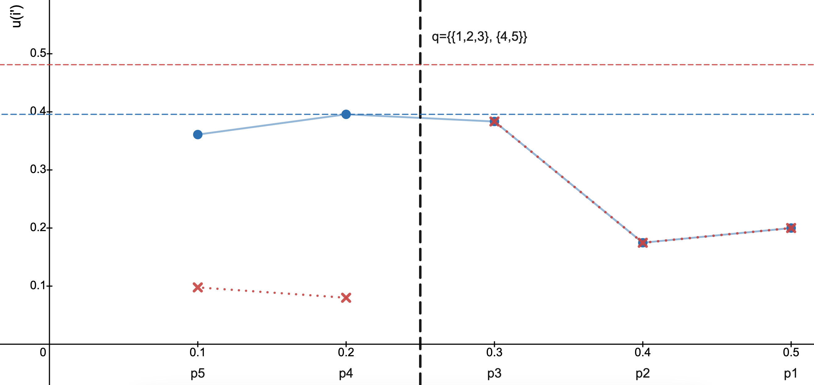
Figure 2: Sender’s expected utility $u(i)$ as a function of the cutoff belief $p_{i}$. The blue solid line represents sender’s utility as a function of the cutoff index when they make no queries. The sender’s optimal utility is given by the blue dashed line. The red dotted line represents sender’s utility as a function of cutoff index when they make the simulation query $q$ which separates the three highest beliefs from the two lowest beliefs. The red dashed line denotes the sender’s ex-ante expected utility from messaging optimally after making query $q$.

4.2 Optimal Querying Policy

Our goal is to identify an optimal querying policy. Queries are helpful for the sender because they refine her information about the beliefs of the receiver. Thus she can target her messaging policy to the receiver she actually faces. Figure 2 demonstrates the impact of a single sender query separating the three highest beliefs from the two lowest ones. The red dotted line represents the sender’s utility as a function of the threshold belief in each resulting information set. This can be weakly less than the sender’s utility before making the query for each individual threshold. However, since the sender’s targeting ability improves, she is able to extract extra utility from low beliefs, improving her overall expected utility ex ante, as represented by the red dashed line.

Recall from Proposition 3.2 that every simulation query corresponds to a threshold query over the space of beliefs. Thus, after any (partial) history of simulation queries and responses, what is revealed to the sender is that the receiver’s belief $p$ lies in some interval $[\theta_{L},\theta_{H}]$. In other words, there are indices $L$ and $H$ such that the receiver’s belief is $p_{i}$ for some $L\leq i\leq H$.

Given a partial history of queries, a simple brute-force algorithm can find the myopically optimal next query in time $O(T^{3})$. Indeed, one can check each possible threshold query that separates beliefs in the range $[L,H]$ (of which there are at most $H-L-1=O(T)$ distinct options), then use the algorithm in Proposition 4.1 to calculate the sender’s optimal messaging policy given each of the two potential responses. This method could be used to greedily construct a sequence of queries one by one, but this may not be optimal. The optimal querying policy might need to make suboptimal queries in some steps to optimize the overall information at the end of the query process. For example, consider an instance of Binary BP with four possible receiver types and $K=2$ simulation queries. In this scenario, it will always be optimal to use the first query to separate the smallest two receiver beliefs from the largest two beliefs, regardless of the immediate utility gain from doing so or any other parameters of the problem instance, since this allows the second query to fully separate all receiver beliefs. Any other initial query is always strictly suboptimal.

In this section, we show that the optimal adaptive querying policy can be computed via dynamic programming. We do this by leveraging the fact that there is a total ordering over receiver beliefs when there are two states. Therefore, we can compute offline an optimal collection of up to $\min\{T,2^{K}-1\}$ possible queries, and thereafter use binary search to construct an adaptive procedure to select the next query given any history of responses. This implies a reduction from the optimal adaptive querying policy to the optimal non-adaptive one.

Definition 4.2 (Non-Adaptive Querying Policy).

A non-adaptive querying policy $\pi$ is described by a set $Q\subset\mathcal{Q}$ of up to $K$ queries (where recall that $K$ is the number of rounds of querying). Policy $\pi$ poses each of the queries in $Q$ in sequence, independently of the history of responses. We call $Q$ the support of policy $\pi$.

Theorem 4.3.

Fix $K\geq 1$ and suppose that $\pi$ is the sender-optimal non-adaptive querying policy with $\min\{T,2^{K}-1\}$ queries. Then there exists a sender-optimal (adaptive) querying policy $\pi^{\prime}$ with $K$ queries that only makes queries in the support of $\pi$. Moreover, $\pi^{\prime}$ can be simulated in time $O(\min\{T,2^{K}\})$ given access to $\pi$.

Proof.

First note that if $2^{K}\geq T$ then the result follows trivially by taking the support of the non-adaptive querying policy to be the set of all possible queries (up to action equivalence). So we will assume that $2^{K}<T$.

Any (adaptive) querying policy $\pi^{\prime}$ with $K$ queries can generate at most $2^{K}$ potential histories, each corresponding to a disjoint subinterval of receiver beliefs implied by the history of responses. These subintervals are described by the at most $2^{K}-1$ thresholds that separate them. One can therefore construct a non-adaptive querying policy $\pi$ with support $Q$ consisting of queries corresponding to each of these thresholds. Querying policy $\pi$ (which makes $2^{K}-1$ queries) would reveal which subinterval contains the receiver’s belief, which is equivalent to the information revealed by policy $\pi^{\prime}$.

We conclude that the optimal non-adaptive policy of length $2^{K}-1$ is at least as informative as the optimal adaptive policy of length $K$. Given the optimal non-adaptive policy $\pi$ of length $2^{K}-1$, its information can be simulated by an adaptive policy $\pi^{\prime}$ of length $K$ via binary search: at each round, $\pi^{\prime}$ selects the query from $Q$ corresponding to the midpoint threshold among all queries in $Q$ that separate types not yet excluded by the history. As this policy results in a distinct subinterval of types for every possible history, it reveals which of the $2^{K}$ subintervals defined by $Q$ contain the receiver’s belief, and is therefore as informative as $\pi$. We conclude that $\pi^{\prime}$ must be optimal among all adaptive policies. ∎

Our problem therefore reduces to finding the best (non-adaptive) set of $\min\{T,2^{K}\}$ queries. We do this using dynamic programming, iteratively building solutions for larger sets of receiver beliefs. We overload notation and use $q$ to index the receiver belief with the smallest prior which takes action $a=1$ in response to simulation query $q\in\mathcal{Q}$. Given a set of $T$ receiver types $\{1,\ldots,T\}$ where $p_{1}>p_{2}>\cdots>p_{T}$, Algorithm 1 keeps track of the optimal sender utility achievable with $k$ queries when in receiver subset $\{1,\ldots,i\}$ for all $1\leq i\leq T$. Due to the structure induced by non-adaptivity in this setting, we are able to write the sender’s expected utility for $k+1$ queries in receiver subset $\{1,\ldots,i+1\}$ as a function of the optimal solution for $k$ queries in subset $\{1,\ldots,i\}$.

Algorithm 1 Computing the Optimal Non-Adaptive Querying Policy: Binary BP, $K$ Queries

Query budget $K\in\mathbb{N}$

• Set

  $$V[i,j]:=\mathbb{E}_{p\sim\mathcal{P}(i,j)}\mathbb{E}_{\omega\sim p}\mathbb{E}_{m\sim\sigma^{*}_{\mathcal{P}(i,j)}(\omega)}\left[u_{S}(\omega,m)\right]$$

  for all $1\leq i\leq j\leq T$, where $\sigma^{*}_{\mathcal{P}(i,j)}$ is the optimal messaging policy of Proposition 4.1 under second-order prior $\mathcal{P}(i,j)$, and $i,j$ is shorthand for types $\{i,\ldots,j\}$.

• For every $1\leq j\leq T$, set $M[j,0]:=V[1,j]$

• For every $1\leq k\leq K$ and $1\leq j\leq T$, compute

  $$M[j,k]:=\max_{q\in\mathcal{Q}}V[q+1,j]+M[q,k-1]$$

• The optimal policy then makes the $K$ queries that obtain value $M[T,K]$.

Theorem 4.4.

In Binary BP with simulation queries, Algorithm 1 computes the sender’s optimal non-adaptive querying policy in $\mathcal{O}(T^{2}K)$ time.

Proof.

The algorithm begins by using Proposition 4.1 to precompute, for each range of receiver beliefs indexed by $[i,j]$ with $i\leq j$, the value of the optimal sender’s messaging policy conditional on the receiver’s belief lying in the given range. These values are stored as $V[i,j]$. We note that this can be done in total time $O(T^{2})$: for each choice of $i$, one can take $L=i$ in the statement of Proposition 4.1, iterate over all $i^{\prime}\geq L$, and evaluate the expression in the argmax of the statement of Proposition 4.1 in update time $O(1)$ per entry. the optimal policy for each $[i=L,j]$ is then determined by the maximum value achieved over all $i^{\prime}\leq j$.

The algorithm next computes $M[j,q]$, for $1\leq j\leq T$ and $0\leq q\leq K$, to be the maximum sender value achievable when the receiver’s belief is known to lie in the index range $[1,j]$ and there are $q$ queries remaining to make. When $q=0$ there are no further queries, so $M[j,0]=V[1,j]$. For $q>0$, we determine $M[j,q]$ by enumerating all possibilities for informative queries (of which there are at most $j\leq T$). As there are $TK$ total entries in $M$, each of which takes $O(T)$ time to compute, our total runtime is $O(T^{2}K)$. ∎

Theorems 4.3 and 4.4 together imply that we can compute the optimal adaptive querying policy in time $O(T^{2}\min\{T,2^{K}\})$.

4.3 Approximately Optimal Querying Policies

Our algorithms for computing the optimal messaging policy (Proposition 3.2) and optimal querying policy (Theorem 4.4) both run in time polynomial in $T$, the number of possible receiver beliefs generated by the signals in $\mathcal{S}$. In this section we show that we can eliminate this dependency on $T$ and instead, for any $\epsilon>0$, compute an $O(\epsilon)$-approximately optimal querying and messaging policy for the sender in time polynomial in $1/\epsilon$. Our approximation will be additive: the sender’s expected payoff under the calculated policies will be at least the optimal expected payoff minus $O(\epsilon)$.

Our approach will be to discretize the space of potential receiver beliefs. To this end, we first study the sensitivity of our policies to errors in receiver beliefs. Let $\mathcal{P}$ be some (possibly continuous) second-order distribution over receiver beliefs. Given any signaling policy $\sigma$, write $V(\sigma,\mathcal{P})$ for the sender’s expected payoff when using signaling policy $\sigma$ for a receiver with belief distributed as $\mathcal{P}$, and let $V^{*}(\mathcal{P})=\max_{\sigma}V(\sigma,\mathcal{P})$. Fixing $\mathcal{P}$, let $\mathcal{P}^{\prime}$ be another second-order belief distribution obtained by “increasing” each receiver belief under $\mathcal{P}$ by up to $\epsilon$, additively. That is, there is a mapping $\eta\colon[0,1]\to[0,1]$ such that (a) $\mathcal{P}^{\prime}$ is the distribution over $\eta(p)$ for $p\sim\mathcal{P}$, and (b) $p\leq\eta(p)\leq p+\epsilon$ for all $p$. Then we claim that changing the distribution of receiver beliefs from $\mathcal{P}$ to $\mathcal{P}^{\prime}$ can only improve the sender’s optimal value, and not by more than $2\epsilon$.

Proposition 4.5.

Let $\mathcal{P}$ and $\mathcal{P}^{\prime}$ be as described above. Then for any messaging policy $\sigma$, $V(\sigma,\mathcal{P})\leq V(\sigma,\mathcal{P}^{\prime})$. Furthermore, $V^{*}(\mathcal{P})\leq V^{*}(\mathcal{P}^{\prime})\leq V^{*}(\mathcal{P})+2\epsilon$.

Proof.

Recall that any policy $\sigma$ is equivalent to one in which each message denotes a threshold belief, above which the receiver should take action $a=1$. A receiver with belief $p_{i}$ that takes action $a=1$ upon receiving a message $m$ will likewise do so if their belief is $p^{\prime}_{i}\geq p_{i}$. Message policy $\sigma$ therefore induces the same distribution over actions taken, conditional on the realization of the state of the world $\omega$. Since $\mathcal{P}^{\prime}$ places weakly more probability on $\omega=1$ for any realization of the receiver’s belief, we conclude that the total probability with which the receiver takes action $a=1$ will only ever increase.

For the second half of the proposition, note that the first half already implies $V^{*}(\mathcal{P})\leq V^{*}(\mathcal{P}^{\prime})$, so it suffices to show that $V^{*}(\mathcal{P}^{\prime})\leq V^{*}(\mathcal{P})+\epsilon$. Let $\sigma^{\prime}$ denote the sender’s optimal messaging policy for $\mathcal{P}^{\prime}$, as characterized by Proposition 4.1, and let $\sigma$ denote the messaging policy for $\mathcal{P}$ under the same choice of $i^{*}$ (from the statement of Proposition 4.1). Then since $p_{i^{*}}$ and $p^{\prime}_{i^{*}}$ differ by at most $\epsilon$, as does the probability of $\omega=1$ under $\mathcal{P}$ and $\mathcal{P}^{\prime}$, we conclude that $V(\sigma,\mathcal{P})\geq V(\sigma^{\prime},\mathcal{P}^{\prime})-\epsilon=V^{*}(\mathcal{P}^{\prime})-2\epsilon$. As $V^{*}(\mathcal{P})\geq V(\sigma,\mathcal{P})$, the result follows. ∎

Proposition 4.5 shows that small perturbations to receiver beliefs cannot influence the sender’s payoff too much at equilibrium. Given second-order belief distribution $\mathcal{P}$ with (possibly continuous) support $\mathcal{T}$, let $\tilde{\mathcal{T}}$ denote a discretized support in which each $p_{i}\in\mathcal{T}$ is rounded down to the nearest multiple of $\epsilon$, and let $\tilde{\mathcal{P}}$ denote the corresponding distribution over these rounded values. Then $|\tilde{\mathcal{T}}|\leq 1/\epsilon$, and by Proposition 4.5 the sender-optimal payoff under $\tilde{\mathcal{P}}$ and under $\mathcal{P}$ differ by at most $2\epsilon$. Applying our algorithms to this discretization of the receiver beliefs yields the following approximate version of our algorithmic results.

Theorem 4.6.

Choose any $\epsilon>0$. In Binary BP with simulation queries, one can compute a querying policy in $O(K\epsilon^{-2})$ time and a messaging policy in $O(\epsilon^{-2})$ time, for which the sender’s expected utility is at least $OPT-\epsilon$, where $OPT$ is the sender’s optimal expected utility at equilibrium.

5 Extensions

5.1 Approximate Oracles

Our baseline model assumes that the query oracle has perfect access to the receiver signal $s$, which it uses to simulate the receiver’s beliefs. However, our results also extend to scenarios where the oracle’s access to the receiver’s belief is imperfect and subject to noise. We show that the sender’s utility will degrade smoothly with the amount of noise in the oracle.

Specifically, suppose that there are constants $\delta,\gamma>0$ such that the following is true. If the receiver has belief $p$, then the query oracle is endowed with a belief $p^{\prime}$ such that $|p^{\prime}-p|<\delta$ with probability at least $1-\gamma$. In this case, we can consider a sender who uses an optimal (or approximately optimal) querying policy as in Theorem 4.4, resulting in a posterior that includes probability $p^{\prime}$. The sender can then reduce each receiver belief in the support of their posterior by $\delta$ before constructing a messaging policy. With probability at least $1-\gamma$, this perturbed posterior will only under-estimate the receiver’s true belief, and only by at most $2\delta$. Thus, by Proposition 4.5, their resulting querying policy generates at most $O(\delta)$ less utility than the optimal policy (i.e., the policy they would have constructed for a perfect oracle), again with probability at least $1-\gamma$. Since the sender’s utility is unconditionally always at least $0$, we obtain the following result.

Proposition 5.1.

Suppose that the receiver’s belief is $p$ and the query oracle simulates a receiver with belief $p^{\prime}$, where $\Pr[|p^{\prime}-p|>\delta]<\gamma$ for some $\delta,\gamma>0$. Then we can compute querying and messaging policies for the sender that obtain expected payoff $(1-\gamma)OPT-O(\delta)$, where $OPT$ is the expected payoff of the optimal policies given access to an oracle for which $p^{\prime}=p$ with probability $1$.

5.2 Partition Queries

The key idea behind Algorithm 1 is that in Binary BP with simulation queries, there is always a “total ordering” over both receiver beliefs and queries, and thus one can use dynamic programming in order to iteratively construct an optimal solution. But simulations, while well-motivated, are a limited type of query. More generally, an oracle might be able to provide information about subsets of beliefs. Specifically, in the most general query model, the sender presents a partition of the belief space and the oracle returns the piece of the partition in which the (true) belief lies. We call such an oracle a partition oracle. With general partition queries, there is no total ordering over beliefs and queries, and so our dynamic program does not extend. In fact, in this section, we show the corresponding decision problem is NP-Complete.

A partition oracle is characterized by the set of allowable queries $\mathcal{Q}$ where each $Q=\{q_{1},\ldots,q_{k}\}\in\mathcal{Q}$ is a partition of the possible receiver beliefs (i.e., $\cup_{i}q_{i}=[0,1]$).

Definition 5.2 (Partition Oracle).

A partition oracle with query space $\mathcal{Q}$ inputs a query $Q\in\mathcal{Q}$ and returns the subset $q\in Q$ such that the receiver’s belief $p\in q$.

The decision problem for finding the optimal querying policy with $K$ rounds is as follows. Given $(\mathcal{T},\mathcal{P},\mathcal{Q},K,u)$ where $\mathcal{T}$ is a set of receiver beliefs, $\mathcal{P}$ is a distribution over receiver beliefs, $\mathcal{Q}$ is a set of allowable queries, $K\in\mathbb{N}$, and $u\in\mathbb{R}_{+}$, does there exist a querying policy $\pi$ such that, after $K$ rounds of interaction with $\pi$, the sender achieves expected utility at least $u$?

To prove NP-Hardness, we reduce from Set Cover. Given a universe of elements $U$, a collection of subsets $S$, and a number $K$, the set cover decision problem asks if there exists a collection of subsets $S^{\prime}\subseteq S$ such that $|S^{\prime}|\leq K$ and $\bigcup_{s\in S^{\prime}}s=U$. Our reduction proceeds by creating a receiver belief for every element in $U$ and a partition query for every subset in $S$. We will define $u$ and $\mathcal{T}=\{p_{i}\}$ in such a way that the sender can only achieve expected utility $u$ if she can distinguish between every pair of receivers; i.e., only if after executing policy $\pi$, the sender knows the receiver’s belief exactly. Finally, we show that under this construction the answer to the set cover decision problem is yes if and only if the answer to the corresponding decision problem is also yes.

Theorem 5.3.

Finding the optimal querying policy is NP-Complete in Binary BP with partition queries.

The following definitions will be useful for the proof of Theorem 5.3.

Definition 5.4 (Belief Partition).

A querying policy $\pi$ induces a partition $\Gamma_{\pi}$ over receiver belief space such that $\bigcup_{\eta\in\Gamma_{\pi}}\eta=\mathcal{T}$. Receiver belief $p$ belongs to the subset $\eta_{\pi}[p]\in\Gamma_{\pi}$ of all receiver beliefs consistent with the history generated by $\pi$ for belief $p$.

Definition 5.5 (Complete Separation).

We say that a querying policy $\pi$ completely separates the set of receiver types $\mathcal{T}$ if, for every receiver belief $p\in\mathcal{T}$,

$$\eta_{\pi}[p]\cap\mathcal{T}=\{p\},$$

where $\eta_{\pi}[p]$ is defined as in Definition 5.4.

We use the shorthand $\texttt{set\_cover}(U,S,K)$ and $\texttt{non-adaptive}(\mathcal{T},\mathcal{P},\mathcal{Q},K,u)$ to refer to the Set Cover and Query decision problems respectively. See 5.3

Proof.

Observe that given a candidate solution $\pi$ and the set of corresponding BIC signaling policies for each receiver subset, we can check whether the sender’s expected utility is at least $u$ in polynomial time, by computing the expectation. This establishes that the problem is in NP. To prove NP-Hardness, we proceed via a reduction from Set Cover. Given an arbitrary Set Cover decision problem $\texttt{set\_cover}(U,S,K)$,

1. Create a set of receiver beliefs $\mathcal{T}(U)$. Specifically, add belief $p_{\varnothing}$ to $\mathcal{T}(U)$, and add a belief $p_{e}$ to $\mathcal{T}(U)$ for every element $e\in U$, where these beliefs will be specified below.

2. For each subset $s\in S$, create a query $q_{s}$ that separates the receiver beliefs $\{p_{e}\}_{e\in s}$ from each other and from all other types $\mathcal{T}(U)\backslash\{p_{e}\}_{e\in s}$. For example if $s=\{1,2,3\}$, then $q_{s}=\{\{p_{1}\},\{p_{2}\},\{p_{3}\},\mathcal{T}(U)\backslash\{p_{1},p_{2},p_{3}\}\}$. Denote the resulting set of queries by $\mathcal{Q}(S)$. Note that each query in $\mathcal{Q}(S)$ has a unique non-singleton set in the partition it induces.

3. Let $\mathcal{P}$ be the uniform prior over $\mathcal{T}(U)$. Set the values $p_{i}$ such that each receiver belief has a different optimal signaling policy. Set $u=\mathbb{E}_{p\sim\mathcal{P}}\mathbb{E}_{\omega\sim p}\mathbb{E}_{m\sim\sigma_{p}^{*}(\omega)}[u_{S}(\omega,a)]$, where $\sigma_{p}^{*}$ is the optimal signaling policy when the receiver is known to have belief $p$.

Part 1:

Suppose $\texttt{set\_cover}(U,S,K)=\texttt{yes}$. Let $S^{\prime}$ denote the set of subsets that covers $S$, and let $\pi$ denote the querying policy that poses queries $\{q_{s}\}_{s\in S^{\prime}}$, in sequence, regardless of the history of responses. Let us consider each $p\in\mathcal{T}$ on a case-by-case basis.

Case 1.1: $p\in\mathcal{T}\backslash\{p_{\varnothing}\}$.

Since $S^{\prime}$ covers $S$, $\{p\}$ is a partition induced by at least one query $q$ made by $\pi$ (by construction), and so $\eta_{\pi}[p]=\{p\}$.

Case 1.2: $p=p_{\varnothing}$.

Likewise, since $S^{\prime}$ covers $S$, for every $p\in\mathcal{T}\backslash\{p_{\varnothing}\}$ there is at least one query $q$ for which $\{p\}$ is a partition induced by $q$. Therefore $p_{\varnothing}$ and $p$ are separated by $q$, which implies $p\not\in\eta_{\pi}[p_{\varnothing}]$. We conclude that $\eta_{\pi}[p_{\varnothing}]=\{p_{\varnothing}\}$.

Putting the two cases together, we see that $\pi$ completely separates $\mathcal{T}(U)$ according to Definition 5.5, and so the sender will be able to determine the receiver’s type and achieve optimal utility. Therefore $\texttt{non-adaptive}(\mathcal{T}(U),\mathcal{P},\mathcal{Q}(S),K,u)=\texttt{yes}$.

Part 2:

Suppose $\texttt{set\_cover}(U,S,K)=\texttt{no}$. Recall that, by construction, for each query $q\in\mathcal{Q}(S)$ there is exactly one response corresponding to a non-singleton set. Fix any querying policy $\pi$ and consider the (unique) history $H$ of queries that is generated by $\pi$ when the response from each query is its unique non-singleton set. Let $\mathcal{Q}^{\prime}$ be the set of $K$ queries posed to the oracle in history $H$. Note that there is a one-to-one mapping between queries in $\mathcal{Q}(S)$ and subsets in $S$, and so we can denote the set of subsets corresponding to $\mathcal{Q}^{\prime}$ by $S^{\prime}:=\{s\}_{q_{s}\in\mathcal{Q}^{\prime}}$. Since $S^{\prime}$ does not cover $S$, there must be at least one element $e_{S^{\prime}}\in S\backslash(\bigcup_{z\in S^{\prime}}z)$. If there are multiple such elements, pick one arbitrarily. Then if the receiver has belief $p_{e_{S^{\prime}}}$, querying policy $\pi$ will generate history $H$. Moreover, by the construction of $\mathcal{Q}$, we know that $p_{e_{S^{\prime}}}$ falls in the same partition as $p_{\varnothing}$ for every $q\in\mathcal{Q}^{\prime}$. Therefore $\eta_{\pi}[p_{\varnothing}]\neq\{p_{\varnothing}\}$, and so $\pi$ does not completely separate $\mathcal{T}(U)$ according to Definition 5.5. Since the sender cannot perfectly distinguish between all receiver types and our choice of $\mathcal{Q}^{\prime}$ was arbitrary, this implies that $\texttt{non-adaptive}(\mathcal{T}(U),\mathcal{P},\mathcal{Q}(S),K,u)=\texttt{no}$. ∎

5.3 Generalized Receiver Utility and Private Types

In our baseline model the receiver’s signal $s$ is private but the receiver’s utility function $u_{R}\colon\Omega\times\mathcal{A}\to\mathbb{R}$ is publicly known. However, our model and results extend to settings where the receiver’s utility is of a more general form that is private knowledge. Specifically, let us assume only that the receiver strictly prefers action $a=\omega$ to action $a\neq\omega$, so that $u_{R}(1,1)>u_{R}(1,0)$ and $u_{R}(0,0)>u_{R}(0,1)$. Then if we write $\mathcal{U}$ for the space of all such utility functions, we can extend our model so that the tuple $(\omega,s,u_{R})$ is drawn from publicly-known distribution $F$ over $\Omega\times\mathcal{S}\times\mathcal{U}$, where only the receiver knows the revelation of $s$ and $u_{R}$. The sender’s simulation oracle will generate responses consistent with both $s$ and $u_{R}$, and therefore reveals information about the tuple $(s,u_{R})$ to the sender. The notion of perfect Bayesian equilibrium in our game is then unchanged, except that the sender forms beliefs over the pair $(s,u_{R})$ rather than over $s$ only.

Under this extension, we can think of a realized pair $(s,u_{R})$ as the type of the receiver. We claim that, just as in our baseline model, any messaging policy is outcome-equivalent to one with at most $T+1$ messages (as in Proposition 3.1), where $T$ is the number of possible receiver types. Moreover, there is a total ordering over the receiver types such that each simulation query is equivalent to a threshold partition query over the space of types with respect to that ordering. To see why, note that the realization of $(s,u_{R})$ induces for the receiver a (prior) belief $p\in[0,1]$ that $\omega=1$. Given a messaging policy $\sigma$ and a realized message $m$, the receiver with prior $p$ will have posterior belief $q=\frac{p\cdot\sigma(m|1)}{p\cdot\sigma(m|1)+(1-p)\cdot\sigma(m|0)}$. The receiver will then take action $a=1$ after seeing message $m$ if and only if

$$q\cdot u_{R}(1,1)+(1-q)\cdot u_{R}(0,1)\geq q\cdot u_{R}(0,1)+(1-q)\cdot u_{R}(0,0)$$

or, equivalently, if and only if

$$\frac{p\cdot\sigma(m|1)}{p\cdot\sigma(m|1)+(1-p)\cdot\sigma(m|0)}=q\geq\frac{u_{R}(0,0)-u_{R}(1,0)}{(u_{R}(1,1)-u_{R}(0,1))+(u_{R}(0,0)-u_{R}(1,0))}$$

which is the same as

$$\sigma(m|0)\leq\sigma(m|1)\cdot\left(\frac{p}{1-p}\cdot\frac{u_{R}(1,1)-u_{R}(0,1)}{u_{R}(0,0)-u_{R}(1,0)}\right).$$

Thus, if we write $\beta=\left(\frac{p}{1-p}\cdot\frac{u_{R}(1,1)-u_{R}(0,1)}{u_{R}(0,0)-u_{R}(1,0)}\right)$, we can associate each receiver with a pair $(p,\beta)$, and write $\mathcal{T}=\{(p_{i},\beta_{i})\}$ for the set of receiver types, ordered so that $\beta_{1}\geq\beta_{2}\geq\dotsc\geq\beta_{T}$. A message $m$ from messaging policy $\sigma$ will induce precisely those receivers with sufficiently high $\beta$ to take action $a=1$. Thus, just as in our baseline model, a simulation query implements a threshold partition query over the space of receiver types, where now the possible receivers are totally ordered by $\beta_{i}$. We note that in our baseline model of receiver utility we have $\beta_{i}=\frac{p_{i}}{1-p_{i}}$, so this is consistent with ordering receivers by their prior belief and with the threshold interpretation of messages from Proposition 3.2.

With this interpretation of messaging policies in hand, we can extend our characterization of the sender’s optimal messaging policy to this scenario with uncertain receiver utilities. The following is the corresponding version of Proposition 4.1 for this extended model.

Proposition 5.6.

[Optimal Messaging Policy] In Binary BP, for a given set of receiver types $\{(p_{i},\beta_{i})\}_{i\in[L,H]}$ with $\beta_{L}>\beta_{L+1}\geq\dotsc\geq\beta_{H}$, the sender’s optimal messaging policy can be computed in time $\mathcal{O}((T^{\prime})^{2})$. The optimal policy is described by an index $i^{*}$ where

$$i^{*}:=\arg\max_{i^{\prime}\in[L,H]}\;\left\{\min\left\{1,\frac{1}{\beta_{i^{\prime}}}\right\}\sum_{i=L}^{i^{\prime}}\mathcal{P}(p_{i})\cdot\left(p_{i}+(1-p_{i})\beta_{i^{\prime}}\right)\right\}.$$

If $\beta_{i^{*}}\leq 1$, the optimal policy is given by $\sigma(m_{i^{*}}|1)=1$, $\sigma(m_{i^{*}}|0)=\beta_{i^{*}}$, and $\sigma(m_{0}|0)=1-\beta_{i^{*}}$; if $\beta_{i^{*}}>1$, the optimal policy is given by $\sigma(m_{i^{*}}|0)=1$, $\sigma(m_{i^{*}}|1)=\frac{1}{\beta_{i^{*}}}$, and $\sigma(m_{H}|1)=1-\frac{1}{\beta_{i^{*}}}$.

The proof of Proposition 5.6 is nearly identical to the proof of Proposition 4.1; the only change is that the incentive constraint for a messaging policy $\sigma$ changes to $\sigma(m_{i}|0)\leq\beta_{i}\sigma(m_{i}|1)$ for each $i$, from the definition of $\beta_{i}$. Note that in our baseline model we have $\beta_{i}=\frac{p_{i}}{1-p_{i}}$ for each $i$, so the policy described above specializes to the one described in Proposition 4.1.

With Proposition 5.6 in hand, one can compute optimal querying policies in precisely the same manner as our baseline model, with receiver types sorted by $\beta_{i}$ rather than $p_{i}$ in the corresponding dynamic program. This leads to the following theorem.

Theorem 5.7.

In Binary BP with simulation queries and uncertain receiver utilities, the sender’s optimal non-adaptive querying policy can be computed in $\mathcal{O}(T^{2}K)$ time.

5.4 Costly Queries

Our model thus far imposed a query budget on the sender. Another natural model would be that the sender can make an unlimited number of queries, but each query comes at a cost to the sender. We note that our main results all extend to this cost model. Extending them requires us to slightly modify the sender’s utility function and the definition of the Bayesian perfect equilibrium. Specifically, if the sender makes queries $q_{1},\ldots,q_{K}$ (for some $K$ chosen by the sender) and the receiver takes action $a$, the sender’s utility is reduced by $\sum_{i}c_{q_{i}}$ where $c_{q_{i}}<1$ is the cost of query $q_{i}$. For any history $H$ of queries and responses observed by the sender, we can write $c(H)$ for the sum of costs of the queries posed in history $H$. The definition of Bayesian perfect equilibrium must change slightly to reflect this utility function, since the sender must account for costs when selecting an optimal query rule. This adds a cost term to the equilibrium condition for query policies. For completeness, we describe the modified equilibrium definition in Appendix A.2.

A dynamic programming algorithm similar to Algorithm 1 may be used to compute the optimal non-adaptive querying policy for the costly setting by (1) setting $K=T-1$, and (2) using the following modified update step:

$$M[j,k]:=\max\{V[1,j],\max_{q\in\mathcal{Q}}V[q+1,j]+M[q,k-1]-c_{q}\}$$

where taking $V[1,j]$ as the maximizer for $M[j,k]$ corresponds to terminating the sequence of queries.

Corollary 5.8.

In the Binary BP setting with costly simulation queries, the above modification to Algorithm 1 computes the sender’s non-adaptive querying policy in $\mathcal{O}(T^{3})$ time.

For the optimal adaptive (i.e., general) querying policy, we note that our reduction to the non-adaptive problem does not directly extend to the costly setting. For example, if the median threshold in the optimal non-adaptive querying policy corresponds to a query with very high cost, it might be suboptimal to make that query first; one might instead begin with a less-balanced but cheaper query and only make the expensive query later in the sequence if necessary.

Nevertheless, another dynamic programming algorithm similar to Algorithm 1 may be used to compute the optimal adaptive querying policy for the costly setting. See Algorithm 2. The primary change relative to Algorithm 1 is that it will maintain a table with entries $M[i,j]$, rather than $M[j,k]$, where $M[i,j]$ denotes the payoff of the sender-optimal querying policy starting from the information that the sender’s belief lies between $p_{i}$ and $p_{j}$. As before, the update step for $M[i,j]$ includes an option to take the maximizer to be $V[i,j]$, which corresponds to the choice to terminate the sequence of queries.

Algorithm 2 Computing the Optimal Adaptive Querying Policy: Binary BP, Costly Queries

Query costs $c_{q}\geq 0$

• Set

  $$V[i,j]:=\mathbb{E}_{p\sim\mathcal{P}(i,j)}\mathbb{E}_{\omega\sim p}\mathbb{E}_{m\sim\sigma^{*}_{\mathcal{P}(i,j)}(\omega)}\left[u_{S}(\omega,m)\right]$$

  for all $1\leq i\leq j\leq T$, where $\sigma^{*}_{\mathcal{P}(i,j)}$ is the optimal messaging policy of Proposition 4.1 under second-order prior $\mathcal{P}(i,j)$, and $i,j$ is shorthand for types $\{i,\ldots,j\}$.

• For every $1\leq i\leq T$, set $M[i,i]:=V[i,i]$

• For every $1\leq i<j\leq T$, compute

  $$M[i,j]:=\max\left\{V[i,j],\max_{q\in\mathcal{Q}}M[i,q]+M[q+1,j]-c_{q}\right\}$$

• The optimal policy then makes the sequence of queries that obtain value $M[1,T]$.

Corollary 5.9.

In the Binary BP setting with costly simulation queries, Algorithm 2 computes the sender’s adaptive querying policy in $\mathcal{O}(T^{3})$ time.

6 Conclusion and Future Work

We initiate the study of information design with an oracle, motivated by recent advances in large language models and generative AI, as well as more traditional settings such as experimentation on a small number of users. We study a setting in which the sender in a Bayesian persuasion problem can interact with an oracle before trying to persuade the receiver, and show how to compute the sender’s optimal adaptive querying policy and subsequent messaging policy. Our algorithm runs in time polynomial in the number of potential receiver beliefs, but can be improved to polynomial in $1/\epsilon$ at the cost of an additive loss of $O(\epsilon)$ for the sender.

There are several exciting directions for future research. First, at a high level, it would be interesting to explore other information design settings in which players have oracle access. While we focus on Bayesian persuasion for its simplicity and ubiquity, it would be natural to ask these same algorithmic design questions in settings such as cheap talk [Crawford and Sobel, 1982] or verifiable disclosure [Grossman and Hart, 1980]. Next, throughout this work, we assumed that the oracle simulates receivers and noted in Section 5.2 that relaxing this to arbitrary partition oracles results in an NP-Complete problem. However, there might be natural subclasses of partition queries, such as interval queries or partitions into few sets, that circumvent this hardness result and are of practical interest. Finally, in this paper, we focused on a Bayesian persuasion setting in which both the state space and action space were binary. Our model extends naturally to settings with multiple states and actions, as described in Section A.1. Simulation queries, rather than being thresholds as in the binary case, become separation oracles as shown in Proposition A.1. However, the outcome of a query is substantially more complex in non-binary settings. In particular, while in the binary case any single query partitions the receiver beliefs into two sets, Example A.2 shows that a single query in the non-binary setting might be sufficient to completely determine the receiver’s belief. It would be interesting to design (approximation) algorithms for this non-binary world.

Appendix A Appendix

A.1 Non-Binary Settings

Suppose there are $|\Omega|>2$ states and $|\mathcal{A}|>2$ actions. By making a simulation query $q=(\sigma_{q},m_{q})$, the sender is specifying a convex polytope $\mathcal{R}_{q}\subseteq\Delta^{d}$ for which we have a separation oracle, a concept from optimization which can be used to describe a convex set. In particular, given a point $\mathbf{x}\in\mathbb{R}^{d}$, a separation oracle for a convex body $\mathcal{K}\subseteq\mathbb{R}^{d}$ will either (1) assert that $\mathbf{x}\in\mathcal{K}$ or (2) return a hyperplane $\boldsymbol{\theta}\in\mathbb{R}^{d}$ which separates $\mathbf{x}$ from $\mathcal{K}$, i.e. $\boldsymbol{\theta}$ is such that $\langle\boldsymbol{\theta},\mathbf{y}\rangle>\langle\boldsymbol{\theta},\mathbf{x}\rangle$ for all $\mathbf{y}\in\mathcal{K}$. Formally, we have the following equivalent characterization of the oracle’s response to a simulation query:

Proposition A.1.

[Relationship between simulation queries and separation oracles] Let

$$\alpha(\mathbf{p}):=\sum_{\omega\in\Omega}(u_{R}(\omega,m_{q})-u_{R}(\omega,a))\cdot\sigma_{q}(m_{q}|\omega)\cdot\mathbf{p}[\omega].$$

By making a simulation query $q=(\sigma_{q},m_{q})$, the sender is specifying a polytope

$$\mathcal{R}_{q}:=\{\mathbf{p}\in\Delta^{d}\;:\;\alpha(\mathbf{p})\geq 0,\forall a\in\mathcal{A}\}$$

and the oracle returns either (i) $\mathbf{p}_{\tau^{*}}\in\mathcal{R}_{q}$ or (ii) $\mathbf{p}_{\tau^{*}}\not\in\mathcal{R}_{q}$ and for some $a^{\prime}\in\mathcal{A}$ for all $\mathbf{p}^{\prime}\in\mathcal{R}_{q}$, $\alpha(\mathbf{p}^{\prime}-\mathbf{p}_{\tau^{*}})>0$.

This is a natural extension of the threshold characterization of simulation queries in the binary setting. However, unlike the binary setting, in this general setting it may be possible to distinguish between three or more beliefs using a single simulation query. Hence the natural generalization of our dynamic program is no longer polynomial time. The following is an example of a setting in which it is possible to distinguish between up to $d$ different beliefs using a single simulation query.

Example A.2.

Suppose that there are $d$ states and $d$ actions, where $u_{R}(\omega,a)=\mathbbm{1}\{\omega=a\}$. Consider $d$ receiver beliefs $\mathbf{p}_{1},\ldots,\mathbf{p}_{d}$ and let $\mathbf{p}_{i}[\omega_{i}]=\frac{2}{d+1}$, $\forall i\in[d]$ and $\mathbf{p}_{i}[\omega_{j}]=\frac{1}{d+1}$ for $j\neq i$. Under this setting, receiver type $i$ will take action $a_{i}$ when $m=a_{1}$ if for all $j\neq 1$,

$$\sigma(a_{1}|\omega_{1})\cdot\frac{2}{d+1}\geq\sigma(a_{1}|\omega_{j})\cdot\frac{1}{d+1}.$$

Therefore, $\mathbf{p}_{1}$ will take action $a_{1}$ when $m=a_{i}$ if for all $j\neq 1$, $\sigma(a_{1}|\omega_{j})=2\sigma(a_{1}|\omega_{1})$. Now let us consider another receiver type $i\neq 1$. Type $i$ will default to taking action $i$ under this messaging policy whenever $m=a_{1}$, since

$$\sigma(m|\omega_{1})\cdot\frac{1}{d+1} <2\sigma(m|\omega_{1})\cdot\frac{2}{d+1}$$

$$\sigma(m|\omega_{1})\cdot\frac{1}{d+1} <2\sigma(m|\omega_{1})\cdot\frac{1}{d+1}$$

where the first line is proportional to how much the receiver loses in expectation by not taking action $i\neq 1$ when recommended action $1$, and the second line is proportional to how much she loses in expectation by not taking action $j\neq i\neq 1$ when recommended action $1$.

A.2 Equilibrium Definition for Costly Queries

In Section 5.4 we described an extension of our model in which the sender must pay to make queries to the receiver simulation oracle. Below we formally define perfect Bayesian equilibrium in this modified model.

Definition A.3.

A profile of strategies $(\pi^{*},\sigma^{*},a^{*})$, together with a belief rule $B_{S}\colon\mathcal{H}\to\Delta(\mathcal{S})$ for the sender mapping query histories to distributions over receiver signals, plus a belief rule $B_{R}\colon\mathcal{M}\times\mathcal{S}\to\Delta(\Omega)$ for the receiver mapping messages and signals to distributions over the state of the world, is a perfect Bayesian equilibrium if:

1. For each $m\in\mathcal{M}$ and $s\in\mathcal{S}$, action $a^{*}(m,s)$ maximizes the receiver’s expected utility given belief $B_{R}(m,s)$:

   $$a^{*}(m)\in\arg\max_{a}\{\mathbb{E}_{\omega\sim B_{R}(m)}[u_{R}(\omega,a)]\}$$

2. Belief $B_{R}(m,s)$ is the correct posterior distribution over $\omega$ given $s$, $\sigma^{*}_{H}$, and the fact that $\sigma^{*}_{H}(\omega)=m$.

3. For each $H\in\mathcal{H}$, messaging policy $\sigma^{*}_{H}$ maximizes the sender’s expected utility given belief $B_{S}(H)$:

   $$\sigma^{*}_{H}\in\arg\max_{\sigma}\{\mathbb{E}_{s\sim B_{S}(H),\omega\sim F|_{s}}[u_{S}(\omega,a^{*}(\sigma(\omega),s))]$$

4. Belief $B_{S}(H)$ is a correct posterior distribution over $s$, given $\pi^{*}$ and the fact that $\pi^{*}$ generates history $H$.

5. Sender’s querying policy $\pi^{*}$ maximizes the sender’s expected utility given $\sigma^{*}$ and $a^{*}$:

   $$\pi^{*}\in\arg\max_{\pi}\{\mathbb{E}_{(\omega,s)\sim F,H\sim\pi}[u_{S}(\omega,a^{*}(\sigma^{*}_{H}(\omega),s))-c(H)]\}$$

References

- [1]
- Aher et al. [2023] Gati Aher, Rosa I. Arriaga, and Adam Tauman Kalai. 2023. Using Large Language Models to Simulate Multiple Humans and Replicate Human Subject Studies. In Proceedings of the 40th International Conference on Machine Learning (Honolulu, Hawaii, USA) (ICML’23). JMLR.org, Article 17, 35 pages.
- Akata et al. [2023] Elif Akata, Lion Schulz, Julian Coda-Forno, Seong Joon Oh, Matthias Bethge, and Eric Schulz. 2023. Playing repeated games with Large Language Models. arXiv preprint arXiv:2305.16867 (2023).
- Audibert et al. [2010] Jean-Yves Audibert, Sébastien Bubeck, and Rémi Munos. 2010. Best Arm Identification in Multi-Armed Bandits. In 23rd Conf. on Learning Theory (COLT). 41–53.
- Balcan et al. [2015] Maria-Florina Balcan, Avrim Blum, Nika Haghtalab, and Ariel D Procaccia. 2015. Commitment without regrets: Online learning in stackelberg security games. In Proceedings of the sixteenth ACM conference on economics and computation. 61–78.
- Bergemann and Morris [2019] Dirk Bergemann and Stephen Morris. 2019. Information Design: A Unified Perspective. Journal of Economic Literature 57, 1 (March 2019), 44–95.
- Bernasconi et al. [2023] Martino Bernasconi, Matteo Castiglioni, Andrea Celli, Alberto Marchesi, Francesco Trovò, and Nicola Gatti. 2023. Optimal rates and efficient algorithms for online Bayesian persuasion. In International Conference on Machine Learning. PMLR, 2164–2183.
- Blum et al. [2014] Avrim Blum, Nika Haghtalab, and Ariel D Procaccia. 2014. Learning optimal commitment to overcome insecurity. Advances in Neural Information Processing Systems 27 (2014).
- Brand et al. [2023] James Brand, Ayelet Israeli, and Donald Ngwe. 2023. Using gpt for market research. Available at SSRN 4395751 (2023).
- Brookins and DeBacker [2023] Philip Brookins and Jason Matthew DeBacker. 2023. Playing Games With GPT: What Can We Learn About a Large Language Model From Canonical Strategic Games? Available at SSRN 4493398 (2023).
- Bubeck et al. [2011] Sébastien Bubeck, Rémi Munos, and Gilles Stoltz. 2011. Pure Exploration in Multi-Armed Bandit Problems. Theoretical Computer Science 412, 19 (2011), 1832–1852.
- Castiglioni et al. [2020] Matteo Castiglioni, Andrea Celli, Alberto Marchesi, and Nicola Gatti. 2020. Online bayesian persuasion. Advances in Neural Information Processing Systems 33 (2020), 16188–16198.
- Castiglioni et al. [2021] Matteo Castiglioni, Alberto Marchesi, Andrea Celli, and Nicola Gatti. 2021. Multi-receiver online bayesian persuasion. In International Conference on Machine Learning. PMLR, 1314–1323.
- Chen et al. [2023] Yiting Chen, Tracy Xiao Liu, You Shan, and Songfa Zhong. 2023. The Emergence of Economic Rationality of GPT. arXiv preprint arXiv:2305.12763 (2023).
- Conitzer and Sandholm [2006] Vincent Conitzer and Tuomas Sandholm. 2006. Computing the optimal strategy to commit to. In Proceedings of the 7th ACM conference on Electronic commerce. 82–90.
- Crawford and Sobel [1982] Vincent P Crawford and Joel Sobel. 1982. Strategic information transmission. Econometrica: Journal of the Econometric Society (1982), 1431–1451.
- Duetting et al. [2023] Paul Duetting, Vahab Mirrokni, Renato Paes Leme, Haifeng Xu, and Song Zuo. 2023. Mechanism Design for Large Language Models. arXiv preprint arXiv:2310.10826 (2023).
- Dworczak and Pavan [2022] Piotr Dworczak and Alessandro Pavan. 2022. Preparing for the worst but hoping for the best: Robust (Bayesian) persuasion. Econometrica 90, 5 (2022), 2017–2051.
- Even-Dar et al. [2006] Eyal Even-Dar, Shie Mannor, and Yishay Mansour. 2006. Action Elimination and Stopping Conditions for the Multi-Armed Bandit and Reinforcement Learning Problems. J. of Machine Learning Research (JMLR) 7 (2006), 1079–1105.
- Fish et al. [2023] Sara Fish, Paul Gölz, David C Parkes, Ariel D Procaccia, Gili Rusak, Itai Shapira, and Manuel Wüthrich. 2023. Generative Social Choice. arXiv preprint arXiv:2309.01291 (2023).
- Grossman and Hart [1980] Sanford J Grossman and Oliver D Hart. 1980. Disclosure laws and takeover bids. The Journal of Finance 35, 2 (1980), 323–334.
- Guo [2023] Fulin Guo. 2023. GPT Agents in Game Theory Experiments. arXiv preprint arXiv:2305.05516 (2023).
- Horton [2023] John J Horton. 2023. Large Language Models as Simulated Economic Agents: What Can We Learn from Homo Silicus? arXiv preprint arXiv:2301.07543 (2023).
- Hu and Weng [2021] Ju Hu and Xi Weng. 2021. Robust persuasion of a privately informed receiver. Economic Theory 72 (2021), 909–953.
- Kamenica [2019] Emir Kamenica. 2019. Bayesian persuasion and information design. Annual Review of Economics 11 (2019), 249–272.
- Kamenica and Gentzkow [2011] Emir Kamenica and Matthew Gentzkow. 2011. Bayesian persuasion. American Economic Review 101, 6 (2011), 2590–2615.
- Kim and Lee [2023] Junsol Kim and Byungkyu Lee. 2023. AI-Augmented Surveys: Leveraging Large Language Models for Opinion Prediction in Nationally Representative Surveys. arXiv preprint arXiv:2305.09620 (2023).
- Kohavi and Longbotham [2017] Ron Kohavi and Roger Longbotham. 2017. Online Controlled Experiments and A/B Testing. In Encyclopedia of Machine Learning and Data Mining, Claude Sammut and Geoffrey I. Webb (Eds.). Springer, Boston, MA, 922–929.
- Kohavi et al. [2009] Ron Kohavi, Roger Longbotham, Dan Sommerfield, and Randal M. Henne. 2009. Controlled experiments on the web: survey and practical guide. Data Min. Knowl. Discov. 18, 1 (2009), 140–181.
- Kolotilin et al. [2017] Anton Kolotilin, Tymofiy Mylovanov, Andriy Zapechelnyuk, and Ming Li. 2017. Persuasion of a privately informed receiver. Econometrica 85, 6 (2017), 1949–1964.
- Kosterina [2022] Svetlana Kosterina. 2022. Persuasion with unknown beliefs. Theoretical Economics 17, 3 (2022), 1075–1107.
- Kovarik et al. [2023] Vojtech Kovarik, Caspar Oesterheld, and Vincent Conitzer. 2023. Game theory with simulation of other players. arXiv preprint arXiv:2305.11261 (2023).
- Letchford et al. [2009] Joshua Letchford, Vincent Conitzer, and Kamesh Munagala. 2009. Learning and approximating the optimal strategy to commit to. In Algorithmic Game Theory: Second International Symposium, SAGT 2009, Paphos, Cyprus, October 18-20, 2009. Proceedings 2. Springer, 250–262.
- Lorè and Heydari [2023] Nunzio Lorè and Babak Heydari. 2023. Strategic Behavior of Large Language Models: Game Structure vs. Contextual Framing. arXiv preprint arXiv:2309.05898 (2023).
- Mannor and Tsitsiklis [2004] Shie Mannor and John N. Tsitsiklis. 2004. The sample complexity of exploration in the multi-armed bandit problem. J. of Machine Learning Research (JMLR) 5 (2004), 623–648.
- Matz et al. [2023] Sandra Matz, Jake Teeny, Sumer S Vaid, Gabriella M Harari, and Moran Cerf. 2023. The Potential of Generative AI for Personalized Persuasion at Scale. PsyArXiv (2023).
- Parakhonyak and Sobolev [2022] Alexei Parakhonyak and Anton Sobolev. 2022. Persuasion without Priors. Available at SSRN 4377557 (2022).
- Park et al. [2023] Joon Sung Park, Joseph C O’Brien, Carrie J Cai, Meredith Ringel Morris, Percy Liang, and Michael S Bernstein. 2023. Generative agents: Interactive simulacra of human behavior. arXiv preprint arXiv:2304.03442 (2023).
- Peng et al. [2019] Binghui Peng, Weiran Shen, Pingzhong Tang, and Song Zuo. 2019. Learning optimal strategies to commit to. In Proceedings of the AAAI Conference on Artificial Intelligence, Vol. 33. 2149–2156.
- Tsuchihashi [2023] Toshihiro Tsuchihashi. 2023. How much do you bid? Answers from ChatGPT in first-price and second-price auctions. Journal of Digital Life 3 (2023).
- Von Stackelberg [1934] Heinrich Von Stackelberg. 1934. Market structure and equilibrium. Springer Science & Business Media.
- Zu et al. [2021] You Zu, Krishnamurthy Iyer, and Haifeng Xu. 2021. Learning to persuade on the fly: Robustness against ignorance. In Proceedings of the 22nd ACM Conference on Economics and Computation. 927–928.