Dynamic Scheduling of a Multiclass Queue in the Halfin-Whitt Regime: A Computational Approach for High-Dimensional Problems
Abstract
We consider a multi-class queueing model of a telephone call center, in which a system manager dynamically allocates available servers to customer calls. Calls can terminate through either service completion or customer abandonment, and the manager strives to minimize the expected total of holding costs plus abandonment costs over a finite horizon. Focusing on the Halfin-Whitt heavy traffic regime, we derive an approximating diffusion control problem, and building on earlier work by Han et al., (2018), develop a simulation-based computational method for solution of such problems, one that relies heavily on deep neural network technology. Using this computational method, we propose a policy for the original (pre-limit) call center scheduling problem. Finally, the performance of this policy is assessed using test problems based on publicly available call center data. For the test problems considered so far, our policy does as well as the best benchmark we could find. Moreover, our method is computationally feasible at least up to dimension 100, that is, for call centers with 100 or more distinct customer classes.
1 Introduction
Motivated by call center operations, this paper considers a dynamic scheduling problem for a multiclass queueing system with a single pool of servers. We focus attention on a finite-horizon, nonstationary formulation in order to model the call center operations over a day and develop an effective computational method to solve it in high-dimensional settings, i.e., for systems with many customer classes. To illustrate the effectiveness of our method, we take a data-driven approach whereby we calibrate our model using data from a large US Bank (see Section 6.1). More specifically, the test problems we study to illustrate the effectiveness of our method are designed and calibrated using the US Bank data set111Our data set is provided by the Service Engineering Enterprise (SEE) Lab at the Technion, and it is publicly available at https://see-center.iem.technion.ac.il/databases/USBank/. Accessed on August 9, 2023..
Call center operations have attracted a significant amount of research attention over the last three decades. The survey papers by Gans et al., (2003) and Aksin et al., (2007) provide an overview through circa 2007; also see Koole and Li, (2023) for a more recent overview. In addition to call center operations, our work blends ideas from three other streams of literature: i) diffusion approximations for queueing systems, ii) stochastic control, and iii) deep learning.
In what follows, we first derive a diffusion approximation of our dynamic scheduling problem. In doing so, we follow the literature that was initiated by the seminal paper Halfin and Whitt, (1981), later extended by Garnett et al., (2002). Halfin and Whitt, (1981) consider a single-class queue with many servers in heavy traffic, where the arrival rate and the number of servers grow large, and the traffic intensity of the system approaches one. Garnett et al., (2002) extend Halfin and Whitt, (1981) to incorporate customer abandonments.
Two important antecedents of our paper in this stream of literature are Harrison and Zeevi, (2004) and Atar et al., (2004). Harrison and Zeevi, (2004) is a multiclass extension of Garnett et al., (2002), where a system manager makes dynamic server allocation decisions to minimize infinite-horizon discounted costs of customer abandonments and holding costs. The authors consider linear holding and abandonment costs and study this problem in the Halfin-Whitt asymptotic regime. They show that the resulting Hamilton-Jacobi-Bellman (HJB) equation admits a smooth solution and numerically solve a two-dimensional example using the finite element method. Atar et al., (2004) follow a similar approach but consider more general cost structures. In addition to showing the existence and uniqueness of a smooth solution to the HJB equation, the authors prove an asymptotic optimality result for the policy they derive from the (formal) limiting control problem; also see Atar, (2005).
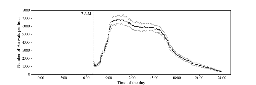
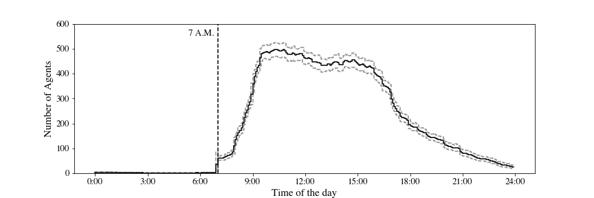
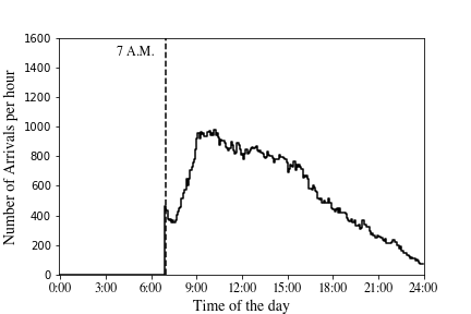
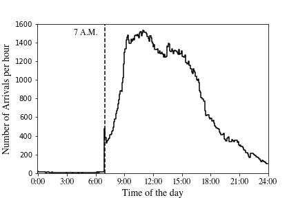
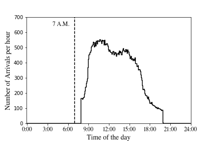
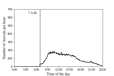
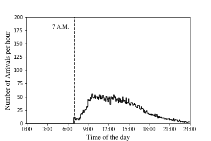
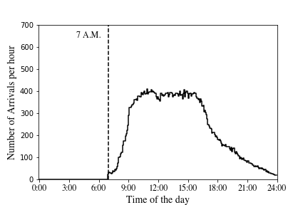
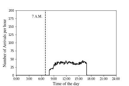
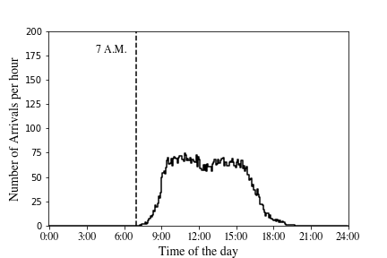
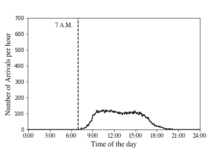
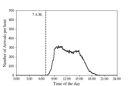
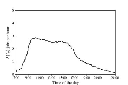
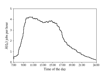
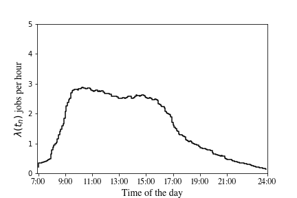
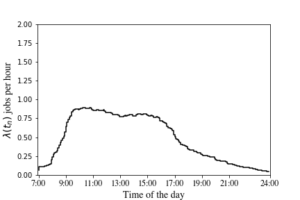
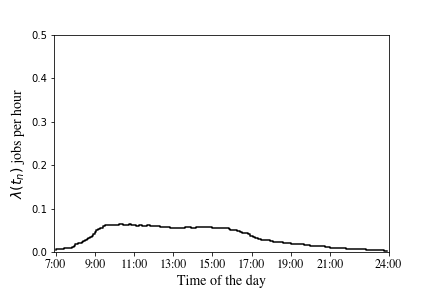
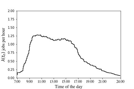
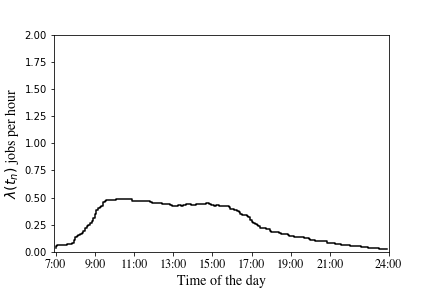
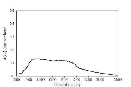
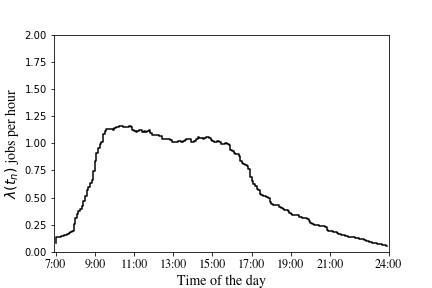
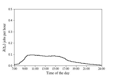
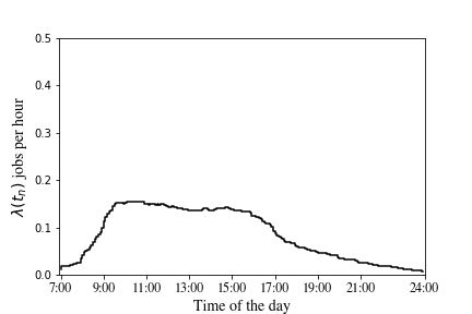
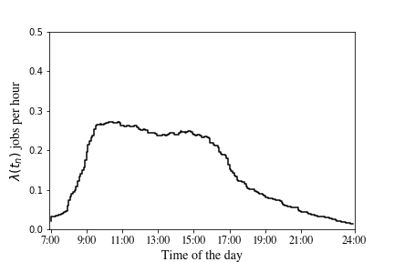
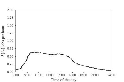
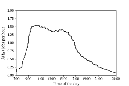
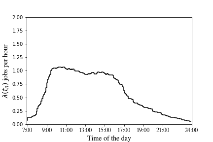
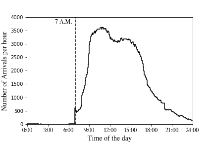
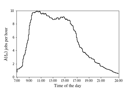
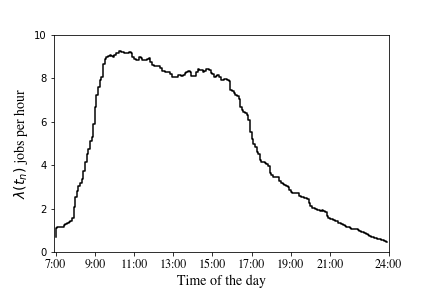
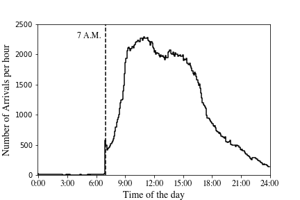
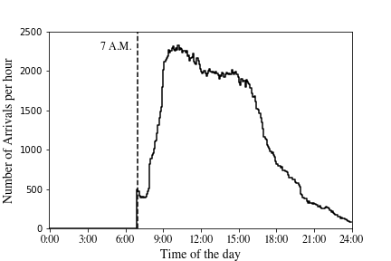
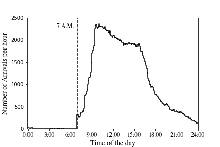
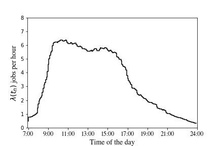
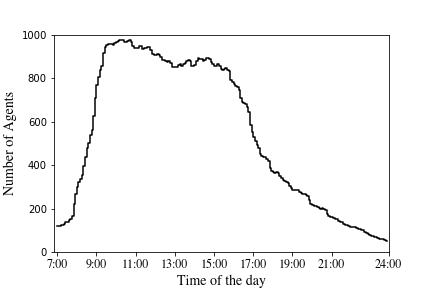
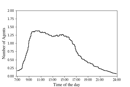
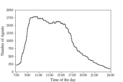
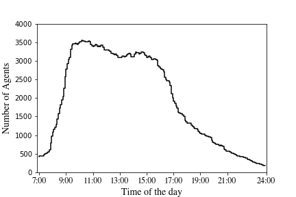
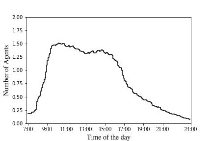
Our formulation is a variation of Harrison and Zeevi, (2004) and Atar et al., (2004) with the main difference being our focus on a finite-horizon formulation with nonstationary data. As mentioned above, all test problems we consider in our extensive numerical study are constructed using the US Bank data. As one would expect, we observe the following in the data: i) both the arrival rates of callers to various classes and the staffing level vary throughout the day, see Figure 1 for a plot of the arrival rate over a day; ii) the number of agents working is in the hundreds during most of the day, with the average number of agents being 273; and iii) the average load factor222The load factor is defined as the ratio of the average amount of work over a specified time to the maximum amount of work that would have been served if the call center had been continuously occupied and it is calculated using Equation (43). of the system is about 90%. These observations led us to choose a nonstationary, finite-horizon model and to study it in the Halfin-Whitt (many-server) asymptotic regime.
Our goal is to develop an effective computational method for solving this problem in high dimensions. To position our work relative to other stochastic systems research, one may recall the framework described by Harrison, (2003) for solving dynamic control problems via diffusion approximations, which we paraphrase as follows:
-
(a)
formulate a conventional stochastic system model with discrete flow units;
-
(b)
define a notion of heavy traffic and formally (that is, non-rigorously) derive a limiting diffusion control problem appropriate for that regime;
-
(c)
solve the diffusion control problem and propose a policy that implements that solution in the original (that is, pre-limit) problem context;
-
(d)
demonstrate the effectiveness of the proposed policy, either by a proof of asymptotic optimality or through a simulation study that compares it against benchmark policies.
Steps (a) and (b) have been successfully executed by Harrison (1988, 2000, 2003) for the conventional heavy traffic regime, and by Atar, (2005) for the Halfin-Whitt regime. Step (d) has also been successfully addressed for various important examples and special cases. For example, Ata and Kumar, (2005) provide asymptotic optimality proofs for policies they derive in the conventional heavy traffic regime, and Atar, (2005) does the same in the Halfin-Whitt regime. In addition, to illustrate the effectiveness of the policies they derived using diffusion approximations, several authors have used simulation studies; see, for example, Harrison and Wein, (1990), Wein, (1992), Chevalier and Wein, (1993) and Ata and Barjesteh, (2023).
In general, step (c) has been a major roadblock for successfully implementing the four-step procedure outlined above, because the HJB equation for the approximating diffusion control problem is a nonlinear partial differential equation (PDE) whose dimension can be high. Historically, the state-of-the-art computational method for solving such PDEs has been the finite-element method, which suffers from the curse of dimensionality. Therefore, solving the HJB equation has only been possible for low dimensional problems: for example, Harrison and Zeevi, (2004) solved a particular two-dimensional problem, while Kumar and Muthuraman, (2004) and Ata et al., (2020) successfully addressed other examples. In this paper, we solve our limiting diffusion control problem in high dimensions, resolving step (c) for our specific context. Using this solution, we propose a policy for the original call center scheduling problem, and show its effectiveness through a simulation study by comparing its performance to that of the best benchmark we could find (see Section 7).
Concurrently, Ata et al., (2023) study drift control of a high-dimensional reflected Brownian motion whose state space is an orthant. Those authors develop a computational method based on earlier research by Han et al., (2018), and while their work differs significantly from ours, it fills a similar gap in the literature. Specifically, by using their method one can execute step (c) of the four-step framework above for a number of dynamic control problems involving stochastic processing networks in the conventional heavy traffic regime.
In order to solve the limiting diffusion control problem, we first express it analytically by considering the associated HJB equation, following the approach that is standard in the stochastic control literature, see Fleming and Soner, (2006). Our HJB equation is a semilinear parabolic partial differential equation, see Gilbarg and Trudinger, (2001). To solve the HJB equation, we follow in the footsteps of Han et al., (2018), who developed a method for solving semilinear PDEs. In doing so, we modify their method, taking into account the special structure of our problem. Similar to Han et al., (2018), our method relies heavily on deep neural network technology; see Section 5. There have been many papers written on solving PDEs using deep neural networks in the last five years; see Beck et al., (2023) and E et al., (2021) for surveys of that literature.
We perform the aforementioned comparison of our proposed policy against benchmarks within the context of several (data-driven) test problems. The US Bank call center data naturally leads to a -dimensional test problem, but this problem is intractable because the associated Markov Decision Process (MDP) suffers from the curse of dimensionality. Additionally, we consider three test problems with dimensions and that are designed so that they have pathwise optimal solutions. Lastly, we consider a two-dimensional test problem as well as two additional test problems that are three-dimensional. Because they are low dimensional, we can solve the original problem by employing the standard techniques for solving the associated MDP.
To repeat, we consider seven test problems. Three of them have pathwise optimal solutions, and we can solve three others using standard techniques for solving MDPs because they are low dimensional. In each of these six cases, our proposed policy performs as well as the optimal policy in the sense that the difference in their performance is not statistically significant. In the 17-dimensional main test problem, the optimal solution is not available. Therefore, we consider a number of benchmark policies (see Section 6.5) and pick the best one. In this problem too, our policy does as well as the best benchmark policy we could find.
The rest of the paper is structured as follows: Section 2 presents the model. Section 3 derives a diffusion approximation in the Halfin-Whitt regime. Section 4 derives a key identity that motivates the loss function used in our learning problem. Section 5 describes our computational method. Section 6 describes the US Bank call center data (Section 6.1), introduces the test problems (Sections 6.2-6.4) and the benchmark policies we use (Section 6.5). All test problems are designed using the US Bank data. Section 7 presents the computational results, comparing the proposed policy against benchmark policies. Appendices A-C provide further details of data, the derivation of the benchmark policies and their computation, as well as how we tuned the neural networks.
2 Model
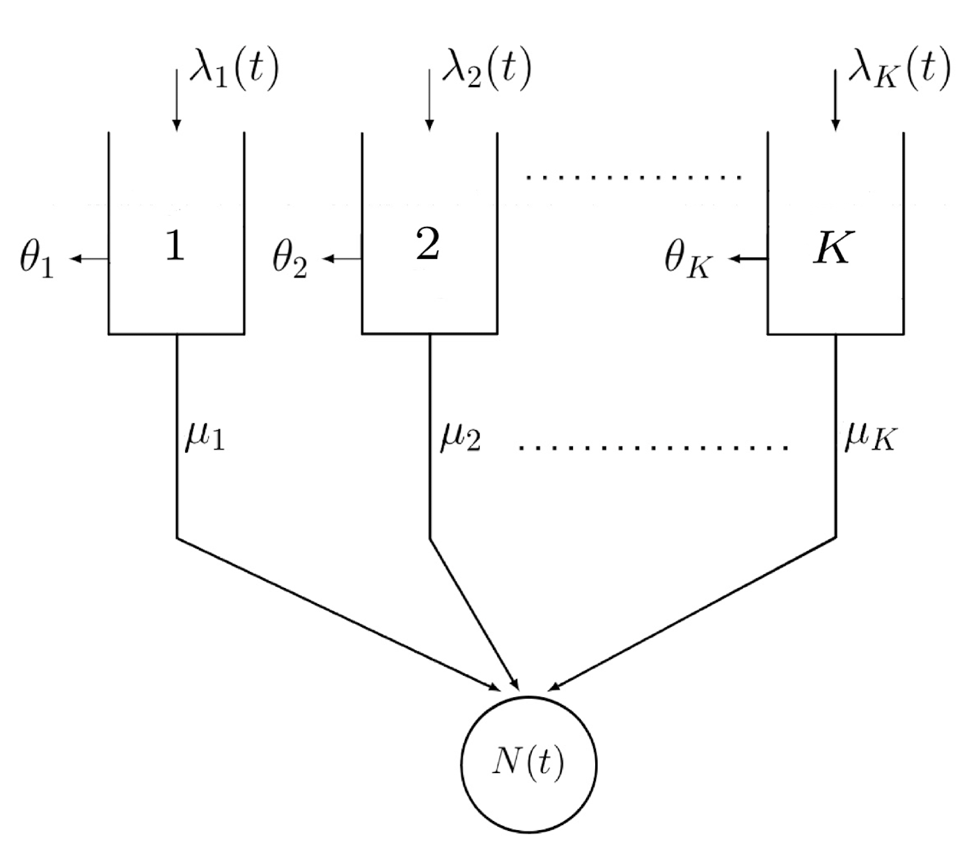
We consider a queueing model of a telephone call center serving classes of callers. Each day, the call center operates during , leading to a finite-horizon formulation. Class callers arrive according to a time-inhomogeneous Poisson process with intensity . They leave the system either by receiving service or by abandoning while they wait in the queue. Associated with each class caller are his service and abandonment times. For class , service times form an i.i.d. sequence of exponential random variables with mean . Similarly, abandonment times of class callers are i.i.d. exponential random variables with mean . The service times, abandonment times, and the caller arrival processes are mutually independent. A schematic description of the model is given in Figure 2.
The system state is denoted by , where denotes the number of class callers in the system. There is a single pool of homogenous agents answering calls. Given the nonstationary nature of arrivals to the call center, the number of agents working varies throughout the day. We let denote the number of agents working at time , and restrict attention to work-conserving policies. That is, an agent does not idle unless all queues are empty.
The system manager decides how to allocate the service effort to callers in the system dynamically. Her control is the -dimensional process , where denotes the number of class callers in service at time . Given system state , the control must satisfy , where
and is the -vector of ones. The requirement follows because the number of class callers in service cannot exceed that in the system for The second requirement ensures that the control is work-conserving. That is, the total number of callers in service is the minimum of the number of servers and the total number of callers in the system.
To facilitate the analysis, we also define two auxiliary processes and as follows: For
| (1) | |||
| (2) |
In words, denotes the number of class callers waiting in the queue at time . Similarly, denotes the number of idle servers at time . The work conservation requirement of an admissible policy can equivalently be expressed as follows:
| (3) |
The system manager strives to minimize the total expected cost that involves holding and abandonment costs incurred during as well as the terminal cost To be more specific, each class caller waiting in queue results in a holding cost rate per unit of time. Similarly, each abandoning class caller costs the system . We define the total cost rate for a class caller in the queue as follows:
| (4) |
Given a control , we characterize the system’s status at time by the triple (. The instantaneous cost rate at time is . Therefore, the total expected cost under policy over the interval , given that , is
| (5) |
where denotes the conditional expectation starting in state under policy . The terminal cost corresponds to the overtime pay associated with serving the callers in the queue at the end of the day. We model it as follows:
| (6) |
where is the overtime pay for an agent to serve a caller in the queue.
The problem described in this section is a continuous-time MDP. In principle, it can be solved using standard dynamic programming techniques. However, that approach is not computationally tractable for problems with high-dimensional state vectors, which is our focus. Therefore, we take a different approach. As a preliminary, we first derive a diffusion approximation to this problem formally (i.e., nonrigorously). We then study the resulting Brownian control problem using a novel computational approach that uses deep neural network approximations.
3 A Brownian control problem in the Halfin-Whitt regime
We consider a sequence of systems, each having the structure described in Section 2, indexed by A superscript of is attached to various quantities of interest to emphasize their dependence on To be specific, we assume the arrival, service, and abandonment rates vary with as follows: For ,
| (7) | |||
| (8) |
where and are given functions. We estimate them from data in Section 6.1 for our test problems. Similarly, the number of agents varies with as follows:
| (9) |
Crucially, we assume that the system primitives satisfy the following heavy traffic assumption:
| (10) |
Combining (7) and (10), the difference between the arriving work and service capacity at each time determines the drift rates for . Under the foregoing assumptions, the system is a balanced, high-volume system. Defining the nominal number of class callers in service (on the fluid scale) as
we now introduce the scaled state, control, queue length, and idleness processes , respectively, as follows: For , and
The scaled control satisfies
The first inequality follows from the natural requirement that and Equations (9) and (10), whereas the second inequality is immediate from , which holds because is admissible for the system. Similarly, Equations (11) - (12) below follow from Equations (1) - (2):
| (11) | |||
| (12) |
In addition, the scaled queue length and idleness processes inherit the following work conservation property from Equation (3):
| (13) |
In what follows, we restrict attention to control policies that satisfy the following:
| (14) |
The leading term on the right-hand side reflects a flow-balance condition. Without it, the system manager incurs costs of order However, for policies that satisfy (14), we expect the costs to be of order The scaling of the second term on the right-hand side is natural under the diffusion scaling we consider.
For such policies, we now derive the infinitesimal drift and covariance of the scaled state process to facilitate our formal derivation of its diffusion limit. In particular, for , , and small , the following holds:
| (15) | |||
| (16) | |||
| (17) |
Passing to the limit formally as and denoting the weak limit of by we deduce from Equations (15) - (17) that the limiting state process satisfies the following: For and
| (18) |
where is a -dimensional standard Brownian motion.
Also, the limiting control, queue length, and idleness processes, , and , respectively, satisfy the following:
| (19) | |||
| (20) | |||
| (21) |
To minimize technical complexity, we restrict attention to Markov controls. Moreover, following Atar et al., (2004), we adopt a choice of control that is more convenient mathematically. To be specific, letting , the system manager chooses a policy , where denotes the fraction of total backlog kept in class at time when the system state is . We let denote the state process under policy . Similarly, the superscript will be attached to various processes to emphasize their dependence on policy as needed for clarity.
Given a policy , one can represent the corresponding (limiting) queue length and idleness processes as follows:
| (22) | |||
| (23) |
Combining Equations (19) and (22) yields
Then for defining
| (24) | |||
| (25) |
and letting and , the following controlled diffusion process describes the limiting state process:
| (26) |
Given a control and the limiting system state , the instantaneous expected cost rate at time is
| (27) |
Therefore, the total expected cost under a policy starting in state at time , denoted by , is given as follows333One can show that is the formal limit of the scaled cost process .:
| (28) |
where and denotes the conditional expectation starting in state under policy . We now define the optimal value function as
where the infimum is taken over the class of admissible policies.
Next, we derive the HJB equation to characterize an optimal Markov policy; see Fleming and Soner, (2006). As a preliminary, we define the differential operator and the function as follows:
Then the HJB equation involves finding a sufficiently smooth function that solves the following partial differential equation: For
where denotes the gradient operator with respect to variable . Rewriting the function more explicitly yields the form of the HJB equation that we will work with: For ,
| (29) | ||||
| (30) | ||||
Similarly, to solve for the total expected cost under an arbitrary policy , a standard argument gives the following PDE: For ,
| (31) |
with the terminal condition
| (32) |
3.1 Optimal policy and its interpretation in the pre-limit system
To characterize the optimal policy, we define the effective holding cost function for class as follows: For ,
| (33) |
Then we define a permutation of such that444Ties are broken by maintaining the order induced by the original class indices.
Class is the most expensive class whereas class is the cheapest one to keep the backlog in at time when the system state is . Thus, the optimal policy, denoted by , keeps the backlog in the cheapest class at all times. That is, for each , it satisfies
Implementing this policy in the pre-limit system literally is not possible. Thus, we propose a natural modification of it. The proposed policy keeps the backlog in the cheapest buffers, that is, the higher indexed classes under permutation , as much as possible. Because we restrict attention to work-conserving policies, this is equivalent to prioritizing lower-indexed classes when assigning servers to callers. To be specific, servers are first assigned to class , then class and so on. That is, given the system state at time , we determine the number of class jobs in service as follows:
4 An equivalent characterization of the value function
In this section, we prove a key identity, Equation (36), which serves as an alternative characterization of the value function . We will later use this identity in Section 5 to define the loss function of our computational method. This identity is closely related to the results of Han et al., (2018), which they use to justify their approach for solving semilinear PDEs. While that earlier work provided inspiration for our study, we include detailed derivations below to ensure that our treatment is self-contained.
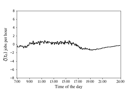
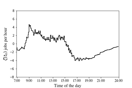
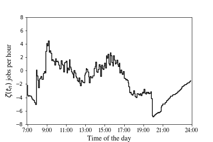
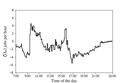
To begin, we specify a reference policy to generate sample paths of the system state. Loosely speaking, we aim to choose a reference policy so that its paths tend to occupy the parts of the state space that we expect the optimal policy to visit frequently. We denote our reference policy by . In our computational study, we consider the following reference policies: i) evenly split, ii) weighted split, iii) minimal, iv) random split, and v) static priority; see Section 5 for details.
The corresponding reference process, denoted by , satisfies the following:
| (34) |
To facilitate the definition of the key identity, let for
| (35) |
Proposition 1.
Proof.
Applying Ito’s formula to on yields
| (37) |
Furthermore, HJB equation (29) yields the following for :
| (38) |
By substituting (38) into (37), employing the terminal condition (30) along with the definition of (Equation (35)) and by writing the integrand of the stochastic integral term in (37) in vector notation, we arrive at the identity (36).
In order to prove the converse, note that taking the expectation of both sides of Equation (36) conditional on gives the following:
In words, can be viewed as the expected total cost associated with the reference process starting in state at time , where the state-cost is at time and the terminal cost is . In other words, corresponds to defined in Equation (28) with in place of . Thus, because satisfies (31) - (32), we conclude that satisfies
| (39) |
for with the terminal condition
| (40) |
Substituting the expressions for (Equation (24)) and (Equation (35)) into Equation (39) implies that solves the following PDE:
| (41) |
for with the terminal condition (40). That is, solves the HJB equation (29) - (30) as desired. ∎
5 Computational method
Our computational method builds on Han et al., (2018), who study a backward stochastic differential equation (BSDE) to motivate the loss function the authors use in their learning problem under a certain neural network approximation. Similarly, we focus on the identity (36) to define our loss function. Given a reference policy, our method first simulates discretized sample paths of the corresponding reference process. To do so, we fix a partition of the time horizon , and simulate discretized sample paths of the reference process at times , see Subroutine 1.
In our numerical study, we consider the following five reference policies: i) evenly split, ii) weighted split, iii) minimal, iv) randomly split, and v) static priority. The evenly split reference policy distributes the backlog evenly across classes. That is, we set for all . The weighted-split reference policy generalizes the evenly-split reference policy slightly. It divides the classes into two sets: and . Then it sets
where and satisfy . If , then the weighted-split reference policy reduces to the evenly-split reference policy. Appendix C describes another particular weighted-split reference policy, where set and weights and are chosen by taking into consideration the call volume of each class. The minimal reference policy sets for all . Under the randomly split reference policy, the backlog is distributed uniformly over the unit simplex. To be more specific, we let be a sequence of i.i.d. Dirichlet () random vectors for and . Lastly, the static priority reference policy puts all backlog in one class. Namely, we pick a class, say and for all and , set the control as follows:
We also considered multiplying the diffusion coefficient by a constant for . This helps the reference policy visit a larger set of states but also increases the training time; see Pham et al., (2021) for further discussion. Not only the choice of the partition is important for simulating discretized sample paths of the reference process, but it affects our neural network approximation crucially. More specifically, we approximate the value function at time zero by a deep neural network with associated parameter vector . Similarly, for , we approximate each gradient function by a deep neural network with parameter vector In particular, the partition of the time horizon determines the number of neural networks we use to approximate the gradient function
We let . Given the neural network parameters , we use a discretized version of the identity (36) to define our loss function, denoted by , as follows:
| (42) | ||||
where and is a Gaussian random vector with zero mean and covariance matrix for . Our method computes the loss, summing over the sampled paths to approximate the expectation, and minimizes it using stochastic gradient descent; see Algorithm 2.
Given the optimal neural network parameters , we use for to approximate the gradient function in defining the proposed policy that we use in our numerical study. More specifically, we approximate the partial derivative with for , and . This leads to the following approximation of the effective holding cost function defined in Equation (33): For , and , we let
Following the approach detailed in Section 3.1, we use the approximate effective holding cost function to order classes from the most expensive to the cheapest. Given this ordering, we propose keeping the backlog in the cheapest buffers as much as possible, as described in Section 3.1. Equivalently, this corresponds to assigning the servers to the “most expensive” class first, then to the second most expensive class, and so on.
6 Data, test problems, and benchmark policies
6.1 Data
We use the publicly available data set of a US bank call center that is provided by the Service Enterprise Engineering Lab at the Technion555Available at https://see-center.iem.technion.ac.il/databases/USBank/. Accessed on August 9, 2023. . The data contains records of agent activities and individual calls between March 2001 and October 2003. The call center operates 24 hours a day, seven days a week, across four sites located in New York, Pennsylvania, Rhode Island, and Massachusetts. Agents are divided into six groups that are referred to as nodes. There isn’t a one-to-one correspondence between nodes and sites. In particular, each node may include agents who are housed in different sites. Similarly, a site may house agents who belong to different nodes. The six nodes are numbered 1, 2, 3, 5, 6, and 7. The call center receives up to 330,000-350,000 calls a day on weekdays and 170,000-190,000 calls a day on weekends. Over a thousand agents work on weekdays and a few hundred on weekends, unevenly distributed among the six different nodes.
Customers enter the system through the voice response unit (VRU), an automated system allowing them to complete transactions independently. Most customers leave the system after performing some self-service transaction via the VRU, but around 55,000-65,000 calls, about 20% of daily arrivals, speak with an agent. We only focus on these callers for our analysis. The VRU forwards these calls to the agents capable of performing the desired service. Over time, the call center stopped some of its services offered in 2001 and started additional services after November 2002. Thus, to focus on the calls that show similar arrival patterns and request the same services, we restrict our analysis to the calls arriving between May and July 2003. During this period, the call center serves 15 different types of customers; see Table 2.
Each call is divided into one or more subcalls that trace its activities in the system from entry to exit. Table 1 lists call characteristics observed in the data. To remove outliers, we focus our analysis on the calls having normal termination, transfer, short abandonment, and abandonment as an outcome, consisting of more than 99% of the observations. Also, we restrict attention to the first subcall, which starts when the customer first joins the queue to speak with an agent and ends when the first service is completed. The total duration of the first subcalls accounts for about 70% of the total talk time of all calls.
| Call ID and ID and the service group of the agent who answered the call |
| Type of service received by the caller |
| Date and time (in seconds) of entering and exiting the queue |
| Date and time (in seconds) of entering and exiting the service |
| The outcome of the call (handled/transferred/abandoned/disconnected/error) |
| Queue time - time a call spends in the queue before entering the service |
| Node - the identifier of the site where the call is being processed |
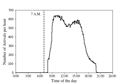
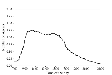
The call volume is significantly higher on weekdays than it is on weekends. We focus attention on weekday calls between 7 A.M. and midnight. Figure 1 shows the call arrival rate during a weekday. The data provides codes for the state of agents for every second of a shift (see Table 11 in Appendix A.1.1). We divide the day into five-minute intervals to find the number of active agents in each interval using this information. We consider an agent to be available in an interval if she is already logged in and has not yet logged out or taken a break. This allows us to determine the number of agents working throughout the day. Since we focus on the first subcalls, we adjust the service capacity allocated to those subcalls according to the time spent on them relative to the total duration of the calls. Figure 3 displays the average number of agents over a day after this adjustment.
As alluded to above, customers who cannot be served immediately after exiting VRU are placed in a queue. These customers can abandon the queue before entering the service. The time to abandon is observed for the callers who abandon. For other callers, the time to abandon is censored by their wait time until they enter service. Only 2% of the callers abandon, leading to heavy censoring of the abandonment times. Such heavy censoring can lead to biased estimates; see Brown et al., (2005) and Akşin et al., (2013). Therefore, we use the bias-corrected Kaplan-Meier estimator proposed by Stute and Wang, (1994) to find the average abandonment times for each service class; see the last column of Table 2.
Finally, to further eliminate outliers, we focus our analysis on the calls with a service time shorter than 30 minutes and a waiting time shorter than 15 minutes, constituting 99.5% of our observations. The Retail class calls that have arrived at nodes 5, 6, and 7 to be served by an agent consist of less than 0.01% of all calls. Thus, we remove these observations from our analysis. Consequently, we focus on three nodes, numbered 1, 2, and 3 for Retail calls. Because the Retail class alone constitutes more than half of all calls, we split it into three different classes corresponding to nodes 1, 2, and 3, where the calls are handled; see the first column of Table 2.
In summary, we focus on 4,016,560 calls from any of the 15 service classes offered by the call center, received on weekdays during May-July 2003, excluding holidays, between 7 A.M. and midnight, having joined the queue to speak with an agent. To repeat, we further restrict attention to their first subcalls. The summary statistics for those calls are given in Table 2.
We supplement the US Bank data by estimating the holding and abandonment costs using other data sources; see Table 3. To do so, we assume the opportunity cost of an hour spent waiting equals the foregone hourly wage of the caller. US Bureau of Labor Statistics666Available at https://www.bls.gov/news.release/empsit.t19.htm. Accessed on August 11, 2023. reports $24 as the average hourly wage for the retail industry. Thus, we set the hourly holding cost rate of the Retail class as $24. Then, we divide the remaining classes into two groups based on their perceived importance/priority relative to the Retail class. Namely, we put classes Premier, Business, Platinum, and Priority Service into one group, and the rest in another group. We further divide the lower priority group into two according to their call volume. For those classes whose arrival rate is less than 1% of the total arrival rate, we set their holding cost rate as $20, the lowest value we use. For the rest of the classes in that group, we set their hourly holding cost rate as $22. Lastly, for those classes in the higher priority group, we set their hourly holding cost rates as shown777Note that the weighted average of the holding cost rates is about $24, the holding cost rate of the Retail class. in Table 3 with Priority Service and Platinum classes having the highest value whereas the Premier class having the lowest value within that group.
| Class | Number of | Arrival | Average service | Average abandonment | ||
|---|---|---|---|---|---|---|
| observations | percentage (%) | time (sec.) | time (sec.) | (per hr.) | (per hr.) | |
| Retail (Node: 1) | 618,077 | 15.39 | 209.04 | 594.30 | 17.22 | 6.06 |
| Retail (Node: 2) | 916,473 | 22.82 | 208.67 | 460.94 | 17.25 | 7.81 |
| Retail (Node: 3) | 622,495 | 15.50 | 208.69 | 689.63 | 17.25 | 5.22 |
| Premier | 138,815 | 3.46 | 273.70 | 367.66 | 13.15 | 9.79 |
| Business | 193,564 | 4.82 | 217.35 | 419.41 | 16.56 | 8.58 |
| Platinum | 13,784 | 0.34 | 209.32 | 480.31 | 17.20 | 7.50 |
| Consumer Loans | 277,930 | 6.92 | 236.95 | 739.10 | 15.19 | 4.87 |
| Online Banking | 106,145 | 2.64 | 339.75 | 644.75 | 10.60 | 5.58 |
| EBO | 28,730 | 0.72 | 364.59 | 437.02 | 9.87 | 8.24 |
| Telesales | 251,513 | 6.26 | 374.20 | 400.25 | 9.62 | 8.99 |
| Subanco | 20,576 | 0.51 | 305.24 | 563.06 | 11.79 | 6.39 |
| Case Quality | 33,652 | 0.84 | 362.71 | 388.48 | 9.93 | 9.27 |
| Priority Service | 58,991 | 1.47 | 347.94 | 393.99 | 10.35 | 9.14 |
| AST | 137,437 | 3.42 | 287.47 | 480.11 | 12.52 | 7.50 |
| CCO | 335,051 | 8.34 | 236.79 | 506.98 | 15.20 | 7.10 |
| Brokerage | 232,338 | 5.78 | 285.30 | 522.39 | 12.62 | 6.89 |
| BPS | 30,989 | 0.77 | 265.27 | 608.49 | 13.57 | 5.92 |
To set the abandonment penalties, we view a caller’s value from service as a proxy for his abandonment penalty. We use the caller’s value of the time spent in service as a proxy for his value for the service. This, in turn, corresponds to his hourly waiting cost divided by 12, because the servers can handle about 12 calls per hour. While admittedly a crude approach, it results in abandonment penalties that are ordered in the same way as the holding costs are ordered, e.g., abandonment penalty for the Platinum class is higher than that for the Retail class.
ZipRecruiter, a popular job listing platform, tracks thousands of salary reports across different industrial sectors. According to their data888Available at https://www.ziprecruiter.com/Salaries/Call-Center-Salary-per-Hour. Accessed on August 12, 2023., the average hourly salary of a call center representative in the U.S. is about $17. Therefore, we use an overtime rate per hour, which corresponds to an overtime rate of per call.
| Class | Arrival | |||
|---|---|---|---|---|
| percentage (%) | (per job) | (per hour) | ||
| Subanco | 0.51 | $1.667 | $20 | |
| EBO | 0.72 | $1.667 | $20 | |
| BPS | 0.77 | $1.667 | $20 | |
| Case Quality | 0.84 | $1.667 | $20 | |
| Online Banking | 2.64 | $1.833 | $22 | |
| AST | 3.42 | $1.833 | $22 | |
| Brokerage | 5.78 | $1.833 | $22 | |
| Telesales | 6.26 | $1.833 | $22 | |
| Consumer Loans | 6.92 | $1.833 | $22 | |
| CCO | 8.34 | $1.833 | $22 | |
| Retail (Node: 1, 2, 3) | 53.71 | $2.000 | $24 | |
| Premier | 3.46 | $2.167 | $26 | |
| Business | 4.82 | $2.500 | $30 | |
| Platinum | 0.34 | $2.667 | $32 | |
| Priority Service | 1.47 | $2.667 | $32 |
6.2 Main test problem
For the main test problem, we set the values of the problem primitives using the US Bank data. Recall that the call center offers 15 different classes of service. Moreover, we split the Retail class into three different classes based on the nodes where the calls are served. Thus, we set the number of classes to and the length of the planning horizon to hours.
Recall that time horizon is partitioned as . We let denote the arrival rate of class during the time interval for , which we estimate from the data; see Figures 11 - 26 of Appendix A.1. We also estimate the mean service and abandonment times, denoted by and respectively, directly from the data; see fourth and fifth columns of Table 2. These yield the limiting service and abandonment rates; see Equation (8). The number of agents working throughout the day estimated from data for each period , denoted by , are displayed in Figure 3. Then we calculate the utilization of the system, denoted by , as follows999For simplicity, we set = for , and the terms in the following equation cancel out.:
| (43) |
Additionally, we set the system parameter , reflecting the order of magnitude for the staffing level, and use it to calculate various limiting parameters that are used crucially in our computational method. To be specific, having determined the system parameter , we define the limiting staffing levels as follows:
| (44) |
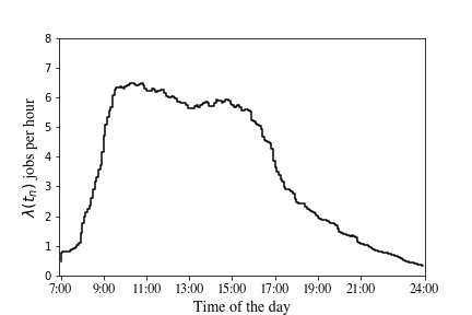
see Figure 61 in Appendix A.1 for the limiting staffing levels throughout the day. In addition, we set the limiting arrival rate for (see Figures 28 - 43 in Appendix A.1) as follows:
| (45) |
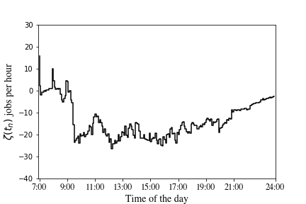
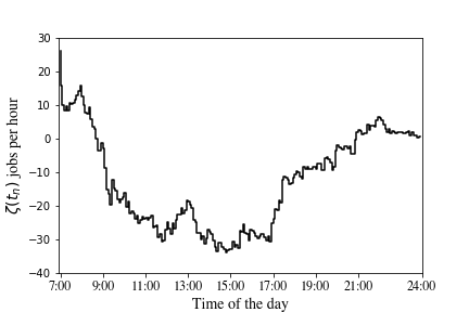
where denotes the fraction of class customers (see the third column of Table 2, also see Equation (10)). We then set the second-order terms using Equation (7) as follows:
| (46) |
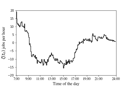
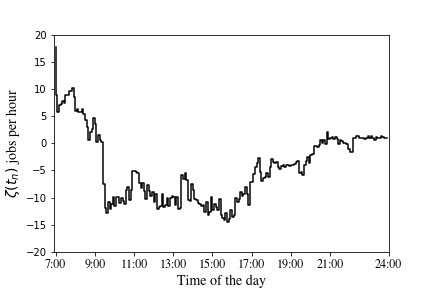
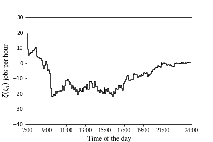
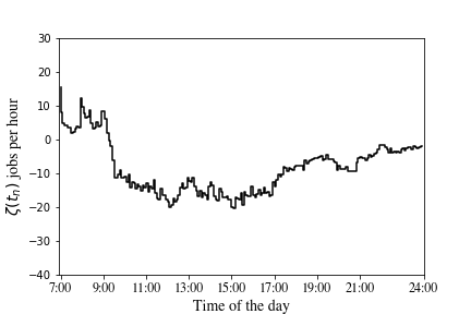
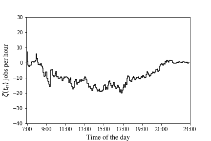
see Figures 45 - 60 in Appendix A.1 for the resulting functions for
Given these primitives of the Brownian control problem, we compute the proposed policy using our method and compare its performance against the benchmark policies introduced in Section 6.5. In doing so, we observed that the rule performs very well among the benchmark policies we considered. Of course, the rule does not always perform well. For example, for the 3-dimensional problem, whose parameters are shown in Table 7, the rule is suboptimal. To be specific, the 95% confidence interval for the cost under the rule for that example is 1684.89 6.36. This corresponds to an optimality gap of 3.65% 0.52%; see the middle column of Table 8 for comparison. In contrast, the performance of our proposed policy is on par with the optimal policy.
6.3 Low dimensional test problems
This section introduces test problems of dimensions . It is computationally feasible to solve such problems using standard MDP techniques. As such, their optimal policies provide natural benchmarks for our proposed policy. To design these test problems, we simply partition the 17 classes into and combine the classes in each group to define a new class; see Table 4 for and Table 5 for for details.
The resulting arrival rates are given in Figure 62 of Appendix A.2.1 for the 2-dimensional test problem and in Figure 65 of Appendix A.2.2 for the 3-dimensional test problem. The mean service and abandonment rates are calculated by taking the weighted average101010The weight of a class is the percentage of arrivals to that class within its group when combining the classes of the main test example. of the rates associated with corresponding classes in the main test example; see Tables 6 - 7. Similarly, we set the hourly holding cost rates , the abandonment cost rates , and the total cost rates by taking the weighted average of the cost rates corresponding classes in the main test example; see the last three columns of the Tables 6 - 7. Also, we use an overtime rate of $2.12 per call, as done in the main test example.
| Class | Names of the Combined Classes | |
|---|---|---|
| 1 | Retail (Node: 2), Business, Telesales, Consumer Loans, | |
| Online Banking, CCO | ||
| 2 | Retail (Node: 1, 3), Premier, Platinum, EBO, Subanco, Case Quality, | |
| Priority Service, AST, Brokerage, BPS |
| Class | Names of the Combined Classes | |
|---|---|---|
| 1 | Retail (Node: 2), Business, Telesales | |
| 2 | Retail (Node: 1), Consumer Loans, Online Banking, CCO | |
| 3 | Retail (Node: 3), Premier, Platinum, EBO, Subanco, Case Quality, | |
| Priority Service, AST, Brokerage, BPS |
The derivation of the limiting quantities follows the same steps as in Section 6.1; see the second columns of Tables 6 - 7 for the updated arrival percentages . Figure 63 in Appendix A.2.1 and Figure 66 in Appendix A.2.2 display the limiting arrival rates for the 2 and 3-dimensional test problems, respectively. Similarly, Figure 64 in Appendix A.2.1 and Figure 67 in Appendix A.2.2 display functions of the 2 and 3-dimensional test problems, respectively.
| Class | Arrival | |||||
|---|---|---|---|---|---|---|
| percentage (%) | (per hr) | (per hr) | (per job) | (per hr) | (per hr) | |
| 1 | 51.80 | 15.32 | 7.40 | $1.97 | $23.63 | $38.20 |
| 2 | 48.20 | 15.49 | 6.45 | $1.99 | $23.83 | $36.64 |
| Class | Arrival | |||||
|---|---|---|---|---|---|---|
| percentage (%) | (per hr) | (per hr) | (per job) | (per hr) | (per hr) | |
| 1 | 33.90 | 15.74 | 8.14 | $2.04 | $24.48 | $41.09 |
| 2 | 33.29 | 15.77 | 6.03 | $1.91 | $22.92 | $34.45 |
| 3 | 32.81 | 14.68 | 6.64 | $1.98 | $23.75 | $36.88 |
A simulation study that considered the six possible static priority policies for the 3-dimensional example revealed that the performance difference between the best and worst static policies was modest (8.07%). Thus, we consider an additional 3-dimensional test example to demonstrate the robustness of our proposed algorithm when the range of expected costs for different policies is larger. Specifically, for the new test problem, all problem primitives of the main 3-dimensional test example remain the same, except for the abandonment penalty , the holding cost rate , and the cost rate for Class 2. As shown in the last three columns of Table 13 in Appendix A.3, these are half of those in the main 3-dimensional test example, cf. Table 7.
6.4 High dimensional test problems
To illustrate the scalability of our method, we introduce three additional test problems of dimensions 30, 50, and 100. We use to distinguish the number of classes of the higher dimensional test problems from that of the main test problem. We also put a on various quantities associated with the new system with classes. To be specific, for each class , we set the arrival rate process by drawing randomly with replacement from the original arrival rate processes ; see Figures 11 - 26 of Appendix A.1 for the latter. The original classes used to determine the arrival rate process are shown in the second column of Tables 14, 15, and 16 in Appendix A.4 for the test problems of dimensions 30, 50, and 100, respectively. Then we use the resulting arrival rate processes to calculate the fraction of class customers in the new system, denoted by , as follows:
| (47) |
Similarly, we set the mean service times and abandonment rates of our test problem, by randomly drawing samples with replacement from the mean service times and abandonment rates independently; see Table 2 for and for .
Recall that denotes the staffing levels throughout the day, estimated directly from the data as shown in Figure 3. In order to determine the staffing levels for the -dimensional problem, we first set the new system parameter as
| (48) |
Then, we set the utilization of the new system denoted by The rationale for this choice is that the larger the system is, the larger the utilization can be without sacrificing system performance due to the statistical economies of scale. In particular, this choice of the system utilization for the large system leads to drift terms of similar magnitudes in the approximating Brownian control problems for the two systems. Given , we then set the staffing levels for the -dimensional problem as follows:
| (49) |
Specifically, to ensure that the staffing level is always integer valued, we round up the calculated values to the nearest whole number by replacing with for . Substituting the system parameter and the estimates of into Equation (44) yields the limiting staffing levels . We set the limiting arrival rate for each class as follows:
so that the heavy traffic condition given in Equation (10) is satisfied. Then we use Equation (46) to estimate the second order terms for each class .
Lastly, we generate a uniform grid of hourly holding cost rates between $14 and $34 with a fixed grid size . The grid size is determined so that the number of possible hourly holding cost rates within this range is greater than or equal to the dimension of the test example111111To be specific, we use values of 0.5, 0.25, and 0.125 for values of 30, 50, and 100, respectively.. Then we randomly draw samples without replacement from this range to determine the hourly holding cost rates .
Crucially, we design these high-dimensional test problems so that they admit pathwise optimal policies. By construction, the classes of these test examples vary from each other only by their arrival, holding cost, and total cost rates. The remaining problem primitives, that is, service times, abandonment rates, and abandonment penalties are the same across different classes121212To determine the common service times, abandonment rates, and abandonment penalties, we take a weighted average of the randomly drawn service times , abandonment rates and holding cost rates .. Further details are provided in Appendix A.4, where Tables 14, 15, and 16 display the system parameters used for the and -dimensional test examples, respectively.
6.5 Benchmark policies
This section introduces the benchmark policies we consider to assess the performance of the proposed policy in each of the seven test problems; see Section 7 for the computational results.
Policies that are pathwise optimal. Recall that three of the seven test problems admit pathwise optimal solutions. Specifically, the three high dimensional cases described in Section 6.4 have pathwise optimal solutions. For these test problems, the optimal policy is the static priority policy that prioritizes classes based on their total cost rates.
Optimal policies for MDP formulations in the low dimensional cases. For the three low dimensional test cases, introduced in Section 6.3, it is computationally feasible to find the optimal policies using standard dynamic programming techniques, which constitute natural benchmarks; see Appendix B.1 for further details.
6.5.1 Benchmark policies for the main test problem
We consider the following benchmark policies for the main test problem: five static priority policies listed below, a policy derived from an auxiliary 3-dimensional MDP that focuses on “low priority” classes described in Appendix B.2.2, and three heuristic dynamic index policies described in Appendix B.2.3.
Static priority rules. Because it is infeasible to search over all possible (17!) static priority policies, we focus on the following subset:
-
1.
The rule proposed by Atar et al., (2010),
-
2.
The rule proposed by Cox and Smith, (1961),
-
3.
The static priority rule based on cost rates ,
-
4.
The static priority rule based on ,
-
5.
The static priority rule based on .
The and rules are well-studied policies and optimal for different models; see Atar et al., (2010) and Cox and Smith, (1961), respectively. The static priority rule based on the cost rates is the pathwise optimal policy for three of our test problems. The last two static priority policies are derived using the definition of the effective holding cost function in Equation (33). To be specific, because we expect /, the higher , the higher the effective holding cost is. Thus, we prioritize the classes with higher overlooking the fact that their cost rate and differs across different classes. The last static rule above also considers the cost rate and ranks classes according to the combined effect, i.e., See Appendix B.2.1 for the performance comparison of the benchmark policies.
7 Computational results
This section compares our proposed policy derived using our computational method (see Section 5) with the benchmark policies introduced in Section 6.5. The performance of our proposed policy is on par with that of the best benchmark in all test problems.
7.1 Results for the low dimensional test problems
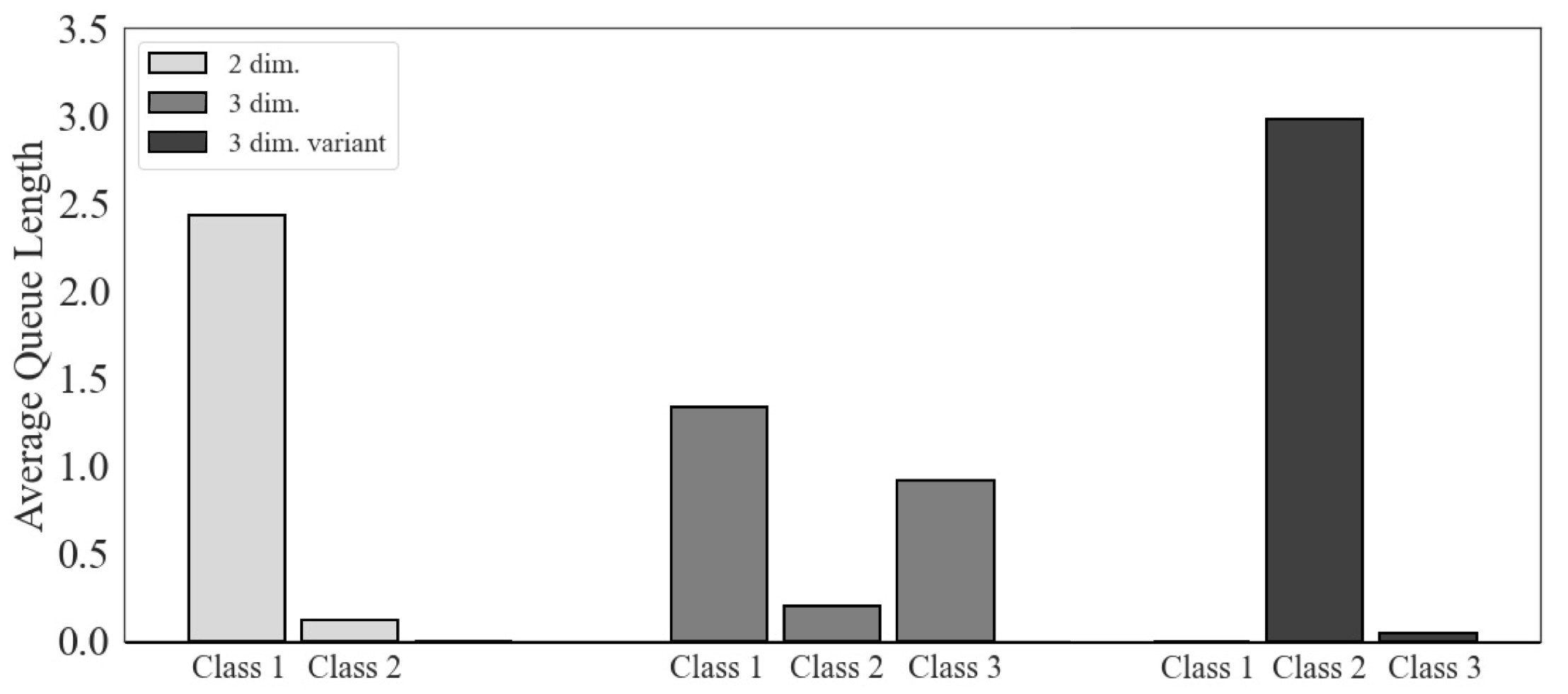
For the low dimensional test problems (), the benchmark policy is the optimal policy computed using standard dynamic programming techniques; see Appendix B.1 for details. Table 8 reports the average total costs obtained in a simulation study131313We use the same random seed for each simulation study with 10,000 replications. All the performance figures reported are subject to simulation and discretization errors. along with the percentage optimality gap between the optimal policy and our proposed policy. They have similar performance. For the last test problem shown in Table 8 (the 3-dimensional variant), the optimal policy is a static priority policy that ranks class 1 highest, class 3 second, and class 2 lowest. Our computational method learns this policy. Because we use common random numbers for comparison, our proposed policy and the benchmark policy have the same performance in all simulation runs done for this test problem.
| Method | 2-Dimensional | 3-Dimensional | 3-Dimensional variant | ||||||||||||
|---|---|---|---|---|---|---|---|---|---|---|---|---|---|---|---|
| Our Policy | 1650.91 6.22 | 1619.95 6.17 | 902.28 3.57 | ||||||||||||
| Benchmark | 1657.96 6.20 | 1623.42 6.18 | 902.28 3.57 | ||||||||||||
| Optimality Gap | -0.43% 0.53% | -0.21% 0.54% | 0% 0.56% |
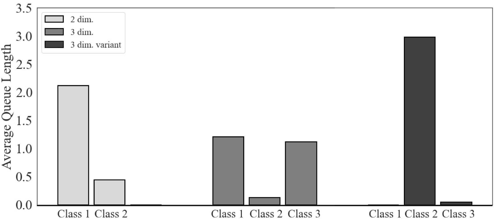
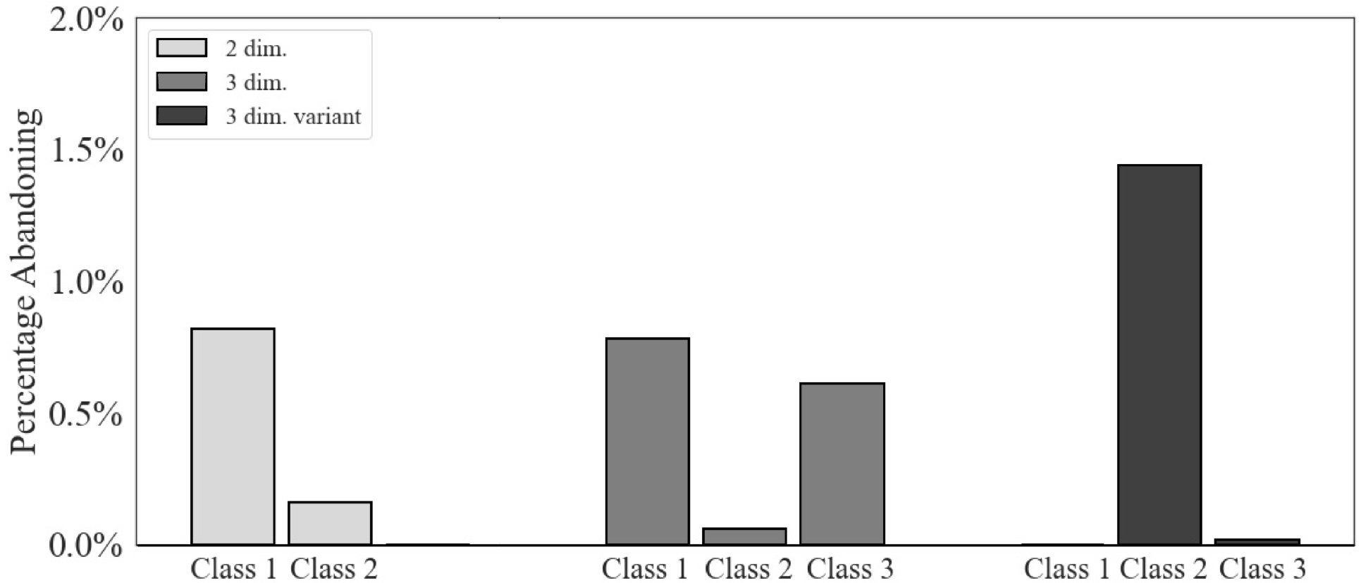
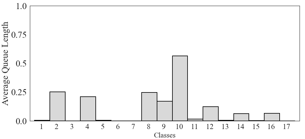
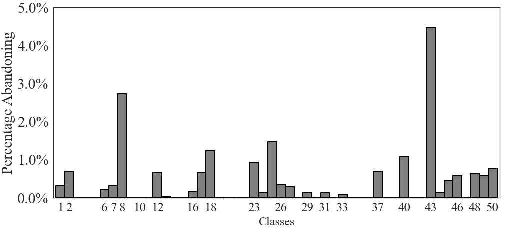
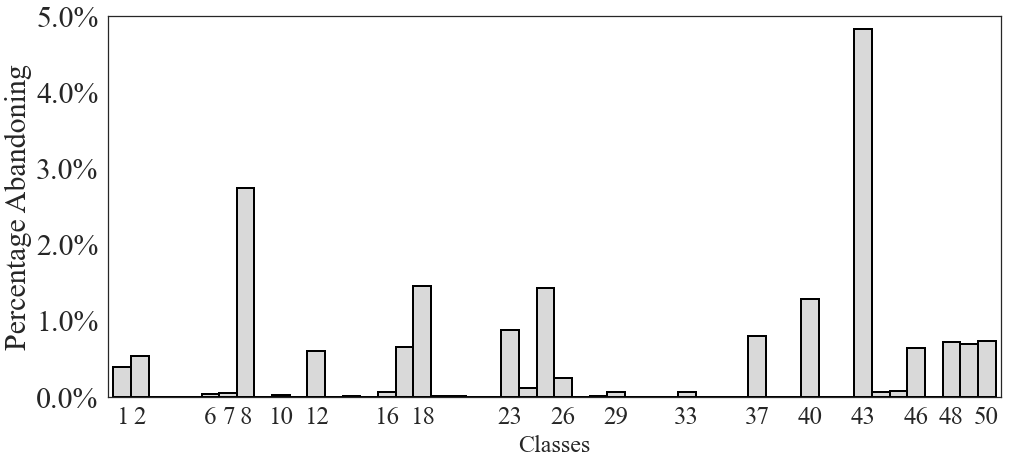
Figures 4 - 5 display how the backlog and the percentage of arrivals that abandon, respectively, are distributed across different classes for the two policies. They show that our proposed policy is similar to the benchmark policy141414Because the abandonment rates are low, the allocation of the service effort is nearly proportional to the offered load of that class under both the benchmark and proposed policies. Thus, the two policies allocate the service effort across different classes similarly..
7.2 Results for the main test problem
For our main test problem (see Section 6.2), the optimal policy is not known, but we consider various benchmark policies (see Section 6.5) and pick the best one to assess the performance of our proposed policy. Table 9 presents the average total costs derived from a simulation study151515We use the same random seed for each simulation study with 10,000 replications. All the performance figures reported are subject to simulation and discretization errors., alongside the percentage optimality gap between the best benchmark policy and our proposed policy.
| Our Policy | Benchmark | Optimality Gap | ||||||||
|---|---|---|---|---|---|---|---|---|---|---|
| 1110.55 4.39 | 1113.93 4.37 | -0.30% 0.56% |
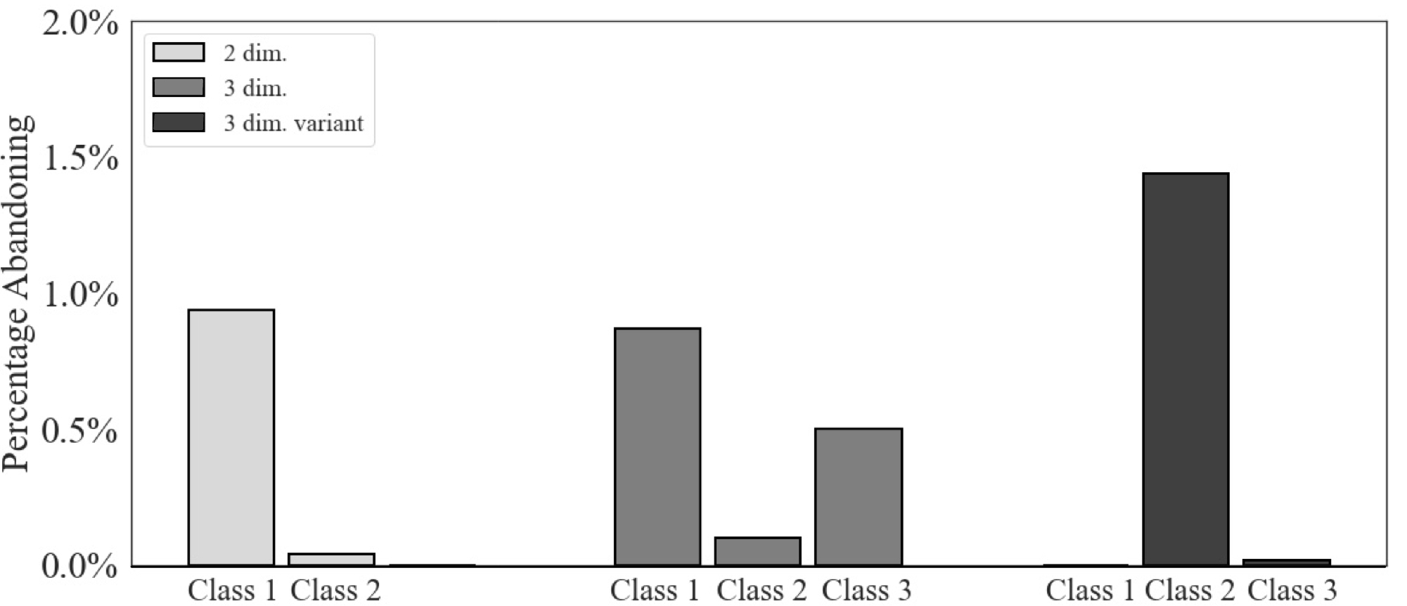
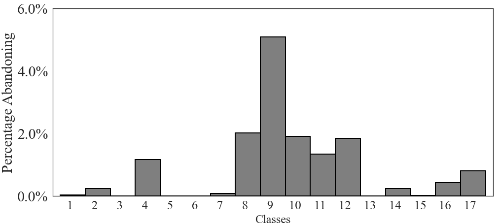
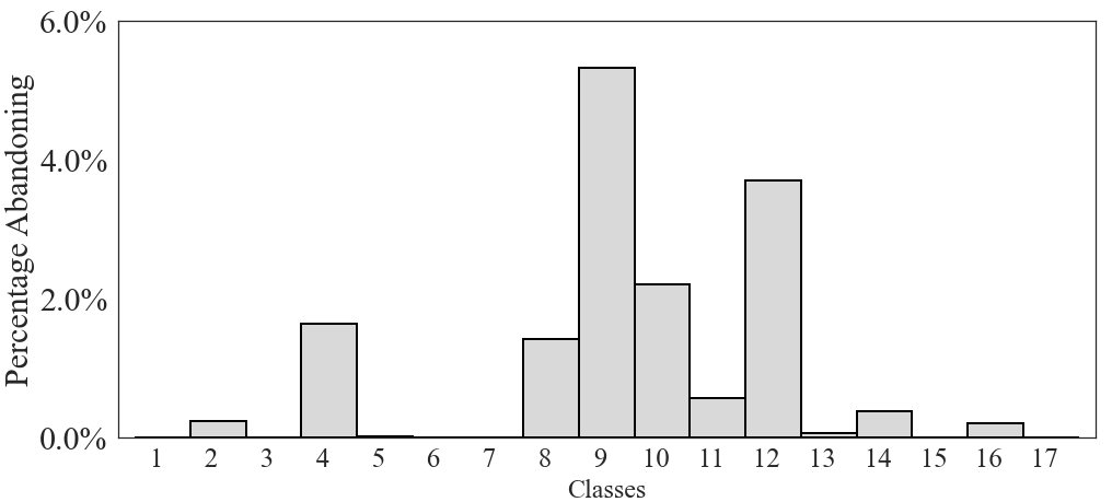
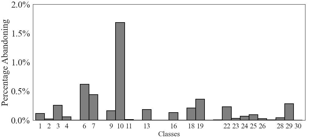
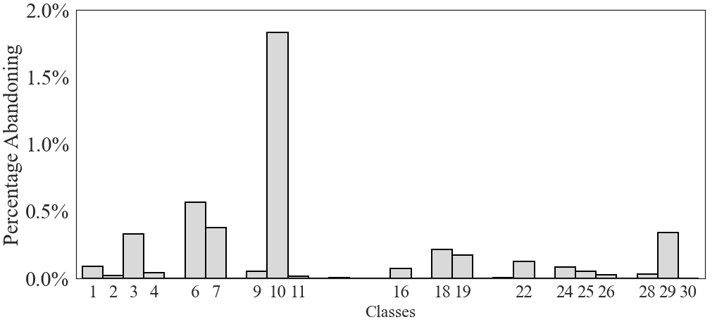
Figures 6 - 7 display how the queue lengths and the percentage of arrivals that abandon, respectively, vary across different classes for the two policies. The numerical results and the figures show that our proposed policy is similar to the benchmark policy for the main test problem.
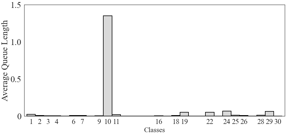
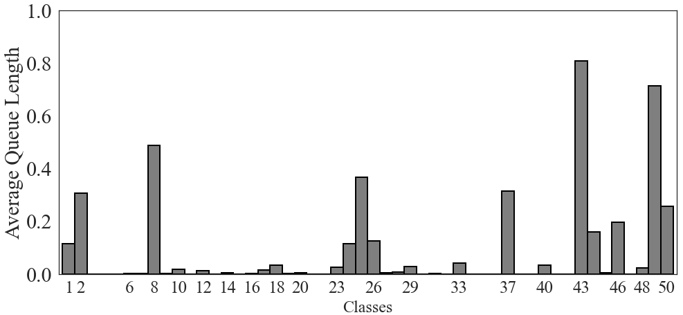
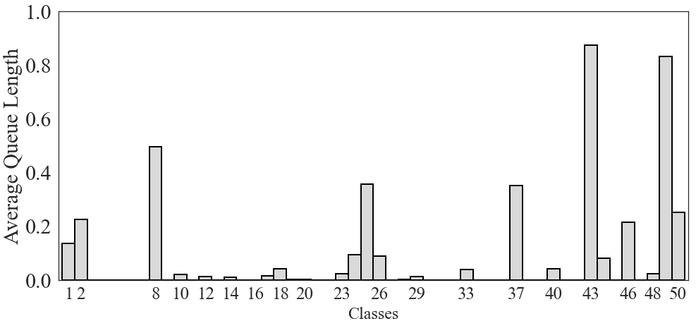
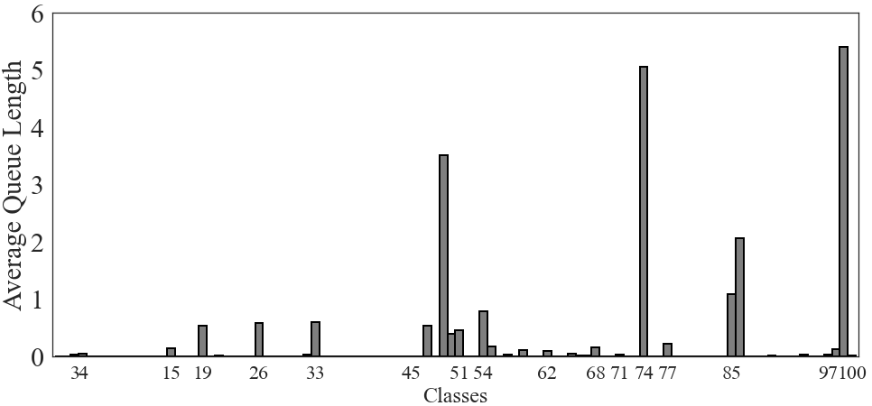
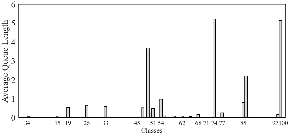
7.3 Results for the high dimensional test problems
The high dimensional test problems introduced in Section 6.4 ( and ) admit pathwise optimal solutions. To be specific, the optimal policy is a static priority policy in each case, and we use it as the benchmark policy. Table 10 reports the simulated performance (average total costs) of our proposed policy and the benchmark policy along with the percentage optimality gap between the two policies. The results show our proposed policy is near optimal. To be more specific, its performance difference from the optimal policy is not statistically significant at the 95% confidence level.
| Method | 30-Dimensional | 50-Dimensional | 100-Dimensional | ||||||||||||
|---|---|---|---|---|---|---|---|---|---|---|---|---|---|---|---|
| Our Policy | 902.03 4.85 | 2386.53 9.22 | 10983.32 16.30 | ||||||||||||
| Benchmark | 896.89 4.78 | 2384.01 9.18 | 10979.24 16.32 | ||||||||||||
| Optimality Gap | 0.57% 0.76% | 0.11% 0.54% | 0.04% 0.21% |
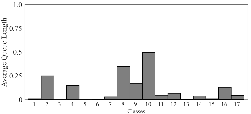
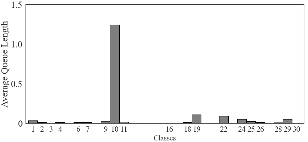
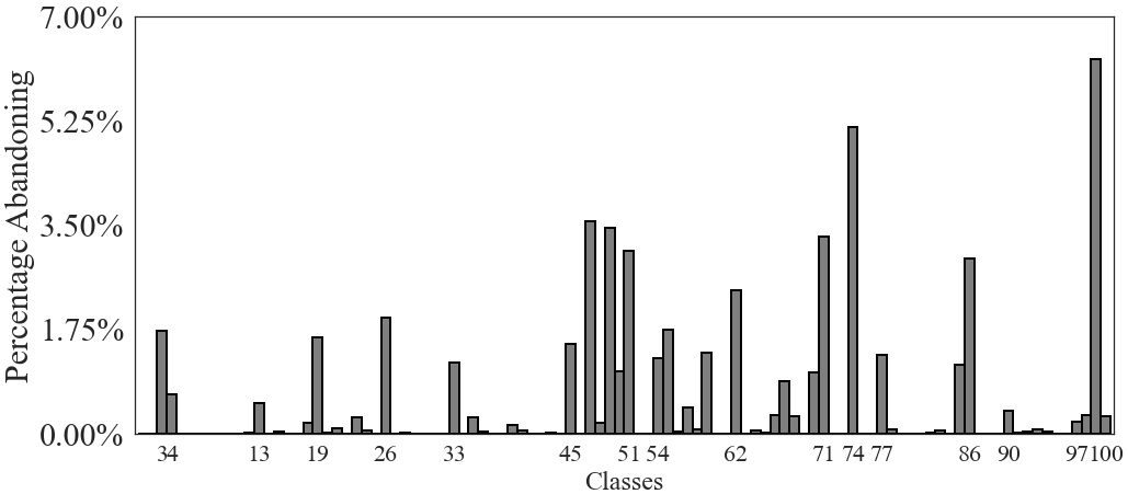
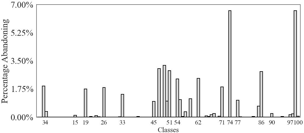
Figures 8 - 9 display how the queue lengths and the percentage of calls that abandon, respectively, vary across different classes for the two policies. They show that our proposed policy is similar to the benchmark policy for each of the test problems considered here.
References
- Abadi et al., (2016) Abadi, M., Barham, P., Chen, J., Chen, Z., Davis, A., Dean, J., Devin, M., Ghemawat, S., Irving, G., Isard, M., and et al. (2016). Tensorflow: A system for large-scale machine learning. In OSDI, volume 16, pages 265–283. Savannah, GA, USA.
- Aksin et al., (2007) Aksin, Z., Armony, M., and Mehrotra, V. (2007). The modern call center: A multi-disciplinary perspective on operations management research. Production and Operations Management, 16(6):665–688.
- Akşin et al., (2013) Akşin, Z., Ata, B., Emadi, S. M., and Su, C.-L. (2013). Structural estimation of callers’ delay sensitivity in call centers. Management Science, 59(12):2727–2746.
- Ata and Barjesteh, (2023) Ata, B. and Barjesteh, N. (2023). An approximate analysis of dynamic pricing, outsourcing, and scheduling policies for a multiclass make-to-stock queue in the heavy traffic regime. Operations Research, 71(1):341–357.
- Ata et al., (2020) Ata, B., Barjesteh, N., and Kumar, S. (2020). Dynamic dispatch and centralized relocation of cars in ride-hailing platforms. Available at SSRN 3675888.
- Ata et al., (2023) Ata, B., Harrison, J. M., and Si, N. (2023). Drift Control of High-Dimensional RBM: A Computational Method Based on Neural Networks. Working Paper, University of Chicago, Booth School of Business.
- Ata and Kumar, (2005) Ata, B. and Kumar, S. (2005). Heavy traffic analysis of open processing networks with complete resource pooling: Asymptotic optimality of discrete review policies. Annals of Applied Probability, 15(1A):331–391.
- Atar, (2005) Atar, R. (2005). Scheduling control for queueing systems with many servers: Asymptotic optimality in heavy traffic. Annals of Applied Probability, 15(4):2606–2650.
- Atar et al., (2010) Atar, R., Giat, C., and Shimkin, N. (2010). The c/ rule for many-server queues with abandonment. Operations Research, 58(5):1427–1439.
- Atar et al., (2004) Atar, R., Mandelbaum, A., and Reiman, M. I. (2004). Scheduling a multi class queue with many exponential servers: Asymptotic optimality in heavy traffic. Annals of Applied Probability, 14(3):1084–1134.
- Atkinson, (1991) Atkinson, K. (1991). An Introduction to Numerical Analysis. 2nd ed. (John Wiley & Sons, New York).
- Beck et al., (2023) Beck, C., Hutzenthaler, M., Jentzen, A., and Kuckuck, B. (2023). An overview on deep learning-based approximation methods for partial differential equations. Discrete and Continuous Dynamical Systems - B, 28(6):3697–3746.
- Bezanson et al., (2017) Bezanson, J., Edelman, A., Karpinski, S., and Shah, V. B. (2017). Julia: A fresh approach to numerical computing. SIAM review, 59(1):65–98.
- Brown et al., (2005) Brown, L., Gans, N., Mandelbaum, A., Sakov, A., Shen, H., Zeltyn, S., and Zhao, L. (2005). Statistical analysis of a telephone call center: A queueing-science perspective. Journal of the American Statistical Association, 100(469):36–50.
- Chevalier and Wein, (1993) Chevalier, P. B. and Wein, L. M. (1993). Scheduling networks of queues: heavy traffic analysis of a multistation closed network. Operations Research, 41(4):743–758.
- Clevert et al., (2016) Clevert, D.-A., Unterthiner, T., and Hochreiter, S. (2016). Fast and Accurate Deep Network Learning by Exponential Linear Units (ELUs). In 4th International Conference on Learning Representations, ICLR 2016 - Conference Track Proceedings.
- Cox and Smith, (1961) Cox, D. R. and Smith, W. (1961). Queues. (Methuen & Co. Ltd, London).
- E et al., (2021) E, W., Han, J., and Jentzen, A. (2021). Algorithms for solving high dimensional PDEs: From nonlinear Monte Carlo to machine learning. Nonlinearity, 35(1):278.
- Fleming and Soner, (2006) Fleming, W. H. and Soner, H. M. (2006). Controlled Markov Processes and Viscosity Solutions. Volume 25. (Springer Science & Business Media, New York).
- Gans et al., (2003) Gans, N., Koole, G., and Mandelbaum, A. (2003). Telephone call centers: Tutorial, review, and research prospects. Manufacturing & Service Operations Management, 5(2):79–141.
- Garnett et al., (2002) Garnett, O., Mandelbaum, A., and Reiman, M. (2002). Designing a call center with impatient customers. Manufacturing & Service Operations Management, 4(3):208–227.
- Gilbarg and Trudinger, (2001) Gilbarg, D. and Trudinger, N. S. (2001). Elliptic Partial Differential Equations of Second Order. 2nd ed., rev. 3rd printing. (Springer, New York).
- Halfin and Whitt, (1981) Halfin, S. and Whitt, W. (1981). Heavy-traffic limits for queues with many exponential servers. Operations Research, 29(3):567–588.
- Han et al., (2018) Han, J., Jentzen, A., and E, W. (2018). Solving high-dimensional partial differential equations using deep learning. Proceedings of the National Academy of Sciences, 115(34):8505–8510.
- Harrison, (1988) Harrison, J. M. (1988). Brownian models of queueing networks with heterogeneous customer populations. In Stochastic Differential Systems, Stochastic Control Theory and Applications, pages 147–186. Springer, New York.
- Harrison, (2000) Harrison, J. M. (2000). Brownian models of open processing networks: Canonical representation of workload. Annals of Applied Probability, 10(1):75–103.
- Harrison, (2003) Harrison, J. M. (2003). A broader view of brownian networks. Annals of Applied Probability, 13(3):1119–1150.
- Harrison and Wein, (1990) Harrison, J. M. and Wein, L. M. (1990). Scheduling networks of queues: Heavy traffic analysis of a two-station closed network. Operations Research, 38(6):1052–1064.
- Harrison and Zeevi, (2004) Harrison, J. M. and Zeevi, A. (2004). Dynamic scheduling of a multiclass queue in the halfin-whitt heavy traffic regime. Operations Research, 52(2):243–257.
- Hochreiter, (1998) Hochreiter, S. (1998). The vanishing gradient problem during learning recurrent neural nets and problem solutions. International Journal of Uncertainty, Fuzziness and Knowledge-Based Systems, 6(02):107–116.
- Innes, (2018) Innes, M. (2018). Flux: Elegant machine learning with julia. Journal of Open Source Software, 3(25):602.
- Koole and Li, (2023) Koole, G. M. and Li, S. (2023). A practice-oriented overview of call center workforce planning. Stochastic Systems, 0(0).
- Kumar and Muthuraman, (2004) Kumar, S. and Muthuraman, K. (2004). A numerical method for solving singular stochastic control problems. Operations Research, 52(4):563–582.
- Pham et al., (2021) Pham, H., Warin, X., and Germain, M. (2021). Neural networks-based backward scheme for fully nonlinear pdes. SN Partial Differential Equations and Applications, 2(1):16.
- Rasamoelina et al., (2020) Rasamoelina, A. D., Adjailia, F., and Sinčák, P. (2020). A review of activation functions for artificial neural networks. In 2020 IEEE 18th World Symposium on Applied Machine Intelligence and Informatics (SAMI), pages 281–286. IEEE.
- Stute and Wang, (1994) Stute, W. and Wang, J.-L. (1994). The jackknife estimate of a kaplan—meier integral. Biometrika, 81(3):602–606.
- Wein, (1992) Wein, L. M. (1992). Dynamic scheduling of a multiclass make-to-stock queue. Operations Research, 40(4):724–735.
Appendix Appendix A Data used for the test problems
For the graphs shown in this section, the resolution of the horizontal axis is 5 minutes. For the main test problem, the graphs follow the order of the class names listed in the first column of Table 2.
Appendix A.1 Main test problem
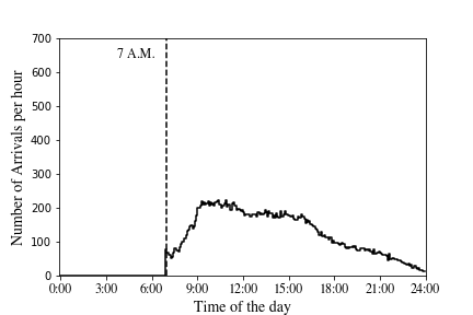
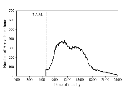
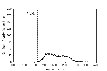
Graphs of the prelimit arrival rates . Figures 11 - 26 display the average hourly arrival pattern for weekday calls of each class during May - July 2003. To improve visibility, we scale the vertical axes of the graphs according to the call volumes161616Using the arrival percentages shown in Table 2, we observe that Retail is the class with the largest call volume. Thus, we set the -axis of Retail class arrivals from 0 to 1600 for each node. For the classes with a medium call volume, we set the -axes from 0 to 700. Lastly, for the classes with the smallest call volume, i.e., the classes with less than 1% aggregate arrival percentage, we set the -axes of the graphs from 0 to 200..
Graphs of the limiting arrival rates . Figures 28 - 43 display the hourly limiting arrival rates for each class , denoted by , which are calculated using Equation (45). To improve visibility, the vertical axes have been scaled relative to the magnitude of the limiting arrival rates171717Specifically, for classes with the highest limiting arrival rates, the y-axes range from 0 to 5. For those with the lowest limiting arrival rates, we set the y-axes from 0 to 0.5. Lastly, for the remaining classes, the y-axes of the graphs are set between 0 and 2..


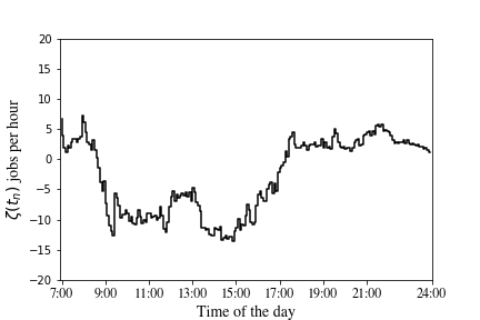
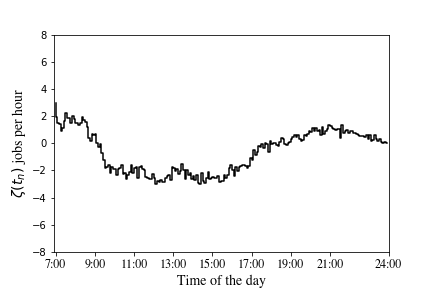
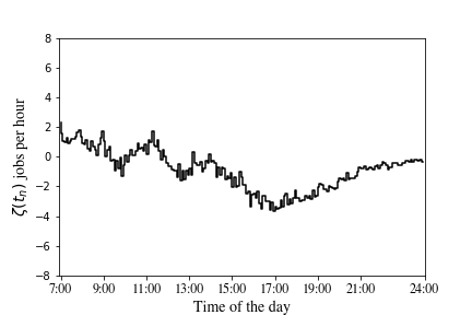
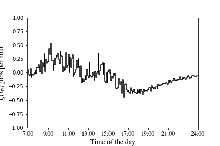
Graphs of the second-order terms . Figures 45 - 60 show the hourly second-order terms , which are calculated using Equation (46). To improve visibility, the vertical axes have been adjusted to reflect the magnitude of the variance of the terms181818To be specific, for the classes with the largest variance in the second-order terms , we set the y-axes from -20 to 20. For those with the smallest variance in the second-order terms , the y-axes of the graphs are set from -8 to 8. For graphs of the remaining classes, the y-axes are set between -1 to 1..


The limiting staffing levels . Substituting the system parameter , and the number of agents , shown in Figure 3, into Equation (44), we find the limiting staffing levels as shown in Figure 61.
Appendix A.1.1 Possible agent states observed in the US Bank call center data
| Code | State | |||
|---|---|---|---|---|
| 1 | Incoming Call | |||
| 2 | Outgoing Call | |||
| 20-21 | Sign-on | |||
| 30-31 | Sign-off | |||
| 40-49 | Idle | |||
| 50 | Available | |||
| 60-62 | Break |
Appendix A.1.2 Data used for the main test problem
| Class | Arrival | |||||
|---|---|---|---|---|---|---|
| percentage (%) | (per hr) | (per hr) | (per job) | (per hr) | (per hr) | |
| Retail (Node: 1) | 15.39 | 17.22 | 6.06 | $2.000 | $24.00 | $36.12 |
| Retail (Node: 2) | 22.82 | 17.25 | 7.81 | $2.000 | $24.00 | $39.62 |
| Retail (Node: 3) | 15.50 | 17.25 | 5.22 | $2.000 | $24.00 | $34.44 |
| Premier | 3.46 | 13.15 | 9.79 | $2.167 | $26.00 | $47.22 |
| Business | 4.82 | 16.56 | 8.58 | $2.500 | $30.00 | $51.46 |
| Platinum | 0.34 | 17.20 | 7.50 | $2.667 | $32.00 | $51.99 |
| Consumer Loans | 6.92 | 15.19 | 4.87 | $1.833 | $22.00 | $30.93 |
| Online Banking | 2.64 | 10.60 | 5.58 | $1.833 | $22.00 | $32.24 |
| EBO | 0.72 | 9.87 | 8.24 | $1.667 | $20.00 | $33.73 |
| Telesales | 6.26 | 9.62 | 8.99 | $1.833 | $22.00 | $38.49 |
| Subanco | 0.51 | 11.79 | 6.39 | $1.667 | $20.00 | $30.66 |
| Case Quality | 0.84 | 9.93 | 9.27 | $1.667 | $20.00 | $35.44 |
| Priority Service | 1.47 | 10.35 | 9.14 | $2.667 | $32.00 | $56.37 |
| AST | 3.42 | 12.52 | 7.50 | $1.833 | $22.00 | $35.75 |
| CCO | 8.34 | 15.20 | 7.10 | $1.833 | $22.00 | $35.02 |
| Brokerage | 5.78 | 12.62 | 6.89 | $1.833 | $22.00 | $34.63 |
| BPS | 0.77 | 13.57 | 5.92 | $1.667 | $20.00 | $29.86 |
Appendix A.2 Low dimensional test problems
Appendix A.2.1 The 2-dimensional test problem
Graphs of the prelimit arrival rates . To determine the hourly arrival rates for the classes of the 2-dimensional test problem, we aggregate the hourly arrival rates of the classes of the main test problem combined into the two new classes as shown in Table 4. Figure 62 displays the hourly arrival pattern for each of the two classes.
Graphs of the limiting arrival rates . Figure 63 shows the hourly limiting arrival rates for each class , denoted by , calculated using Equation (45).
Graphs of the second-order terms . Figure 64 shows the hourly second-order terms, denoted by , which are calculated using Equation (46).
Appendix A.2.2 3-dimensional test problems
Recall that the two test problems we consider (that are three-dimensional) differ only in their cost parameters.
Graphs of the prelimit arrival rates . To set the hourly arrival rates of the classes for the 3-dimensional test problem, we aggregate the hourly arrival rates of the classes of the main test problem according to the class definitions provided in Table 5. Figure 65 illustrates the hourly arrival patterns for each of these three classes.
Graphs of the limiting arrival rates . Figure 66 shows the hourly limiting arrival rates for each class , denoted by , calculated using Equation (45).

Graphs of the second-order terms . Figure 67 shows the hourly second-order terms, denoted by , which are calculated using Equation (46).
Appendix A.3 Data used for 3-dimensional variant test problem
| Class | Arrival | |||||
|---|---|---|---|---|---|---|
| percentage (%) | (per hr) | (per hr) | (per job) | (per hr) | (per hr) | |
| 1 | 33.90 | 15.74 | 8.14 | $2.04 | $24.48 | $41.09 |
| 2 | 33.29 | 15.77 | 6.03 | $0.96 | $11.46 | $17.23 |
| 3 | 32.81 | 14.68 | 6.64 | $1.98 | $23.75 | $36.88 |
Appendix A.4 Data used for the high dimensional test problems
Tables 14, 15, and 16 describe the system parameters used for the test problems of dimensions of 30, 50, and 100, respectively. The second column of the tables lists the names of the classes from the main test problem that are used to set the arrival rate process . Additionally, the tables provide information on the arrival percentages, denoted by , common hourly service and abandonment rates, and abandonment penalty, denoted by , and , respectively. These common problem primitives are determined by taking a weighted average of randomly drawn service rates, abandonment rates, and abandonment penalties from the main test problem. The last two columns in each table present the hourly holding cost rates and total hourly cost rates for each class . As explained in Section 6.4, the classes differ from each other only by their arrival, holding cost, and total cost rates. The holding cost rates are randomly drawn from a uniform grid between $14 and $34, with mesh sizes of and for test problems of size and , respectively.
Appendix A.4.1 The 30-dimensional test problem
The prelimit staffing levels and the limiting staffing levels . We use Equation (49) to find the prelimit staffing levels for the 30-dimensional problem. Substituting the prelimit staffing levels and the system parameter into Equation (44), we find the limiting staffing levels . Figure 68 displays the prelimit staffing levels and the limiting staffing levels throughout the day.
| Class | Arrivals | Arrival | |||||
|---|---|---|---|---|---|---|---|
| sourced from | percentage (%) | (per hr) | (per hr) | (per job) | (per hr) | (per hr) | |
| 1 | Consumer Loans | 3.77 | 14.07 | 7.80 | $1.97 | $15.50 | $30.86 |
| 2 | CCO | 4.54 | 14.07 | 7.80 | $1.97 | $20.50 | $35.86 |
| 3 | Subanco | 0.28 | 14.07 | 7.80 | $1.97 | $21.50 | $36.86 |
| 4 | Online Banking | 1.44 | 14.07 | 7.80 | $1.97 | $24.00 | $39.36 |
| 5 | Consumer Loans | 3.77 | 14.07 | 7.80 | $1.97 | $30.50 | $45.86 |
| 6 | Subanco | 0.28 | 14.07 | 7.80 | $1.97 | $16.50 | $31.86 |
| 7 | Subanco | 0.28 | 14.07 | 7.80 | $1.97 | $20.00 | $35.36 |
| 8 | Premier | 1.88 | 14.07 | 7.80 | $1.97 | $33.00 | $48.36 |
| 9 | Online Banking | 1.44 | 14.07 | 7.80 | $1.97 | $23.50 | $38.86 |
| 10 | Retail (Node: 3) | 8.44 | 14.07 | 7.80 | $1.97 | $14.50 | $29.86 |
| 11 | Retail (Node: 2) | 12.38 | 14.07 | 7.80 | $1.97 | $25.00 | $40.36 |
| 12 | Case Quality | 0.46 | 14.07 | 7.80 | $1.97 | $31.50 | $46.86 |
| 13 | Platinum | 0.19 | 14.07 | 7.80 | $1.97 | $27.00 | $42.36 |
| 14 | Retail (Node: 2) | 12.38 | 14.07 | 7.80 | $1.97 | $32.00 | $47.36 |
| 15 | Retail (Node: 1) | 8.38 | 14.07 | 7.80 | $1.97 | $29.50 | $44.86 |
| 16 | Case Quality | 0.46 | 14.07 | 7.80 | $1.97 | $22.50 | $37.86 |
| 17 | Case Quality | 0.46 | 14.07 | 7.80 | $1.97 | $30.00 | $45.36 |
| 18 | BPS | 0.42 | 14.07 | 7.80 | $1.97 | $18.50 | $33.86 |
| 19 | Telesales | 3.41 | 14.07 | 7.80 | $1.97 | $16.00 | $31.36 |
| 20 | Brokerage | 3.09 | 14.07 | 7.80 | $1.97 | $28.50 | $43.86 |
| 21 | CCO | 4.54 | 14.07 | 7.80 | $1.97 | $24.50 | $39.86 |
| 22 | CCO | 4.54 | 14.07 | 7.80 | $1.97 | $15.00 | $30.36 |
| 23 | Case Quality | 0.46 | 14.07 | 7.80 | $1.97 | $27.50 | $42.86 |
| 24 | Retail (Node: 3) | 8.44 | 14.07 | 7.80 | $1.97 | $22.00 | $37.36 |
| 25 | Business | 2.62 | 14.07 | 7.80 | $1.97 | $23.00 | $38.36 |
| 26 | Consumer Loans | 3.77 | 14.07 | 7.80 | $1.97 | $19.00 | $34.36 |
| 27 | EBO | 0.39 | 14.07 | 7.80 | $1.97 | $29.00 | $44.36 |
| 28 | Consumer Loans | 3.77 | 14.07 | 7.80 | $1.97 | $17.50 | $32.86 |
| 29 | Premier | 1.88 | 14.07 | 7.80 | $1.97 | $19.50 | $34.86 |
| 30 | AST | 1.86 | 14.07 | 7.80 | $1.97 | $31.00 | $46.36 |
Appendix A.4.2 The 50-dimensional test problem
The prelimit staffing levels and the limiting staffing levels . We use Equation (49) to find the prelimit staffing levels for the 50-dimensional problem. Substituting the prelimit staffing levels and system parameter into Equation (44), we find the limiting staffing levels . The prelimit staffing levels and the limiting staffing levels throughout the day are shown in Figure 69.

Appendix A.4.3 The 100-dimensional test problem
The prelimit staffing levels and the limiting staffing levels . We use Equation (49) to find the prelimit staffing levels for the 100-dimensional problem. Substituting the prelimit staffing levels and system parameter into Equation (44), we find the limiting staffing levels . The prelimit staffing levels and the limiting staffing levels throughout the day are shown in Figure 70.
| Class | Arrivals | Arrival | |||||
|---|---|---|---|---|---|---|---|
| sourced from | percentage (%) | (per hr) | (per hr) | (per job) | (per hr) | (per hr) | |
| 1 | Consumer Loans | 2.12 | 13.69 | 7.14 | $2.08 | $17.75 | $32.58 |
| 2 | CCO | 2.56 | 13.69 | 7.14 | $2.08 | $16.25 | $31.08 |
| 3 | Subanco | 0.16 | 13.69 | 7.14 | $2.08 | $31.75 | $46.58 |
| 4 | Online Banking | 0.81 | 13.69 | 7.14 | $2.08 | $33.75 | $48.58 |
| 5 | Consumer Loans | 2.12 | 13.69 | 7.14 | $2.08 | $30.75 | $45.58 |
| 6 | Subanco | 0.16 | 13.69 | 7.14 | $2.08 | $25.50 | $40.33 |
| 7 | Subanco | 0.16 | 13.69 | 7.14 | $2.08 | $24.00 | $38.83 |
| 8 | Premier | 1.06 | 13.69 | 7.14 | $2.08 | $18.25 | $33.08 |
| 9 | Online Banking | 0.81 | 13.69 | 7.14 | $2.08 | $26.00 | $40.83 |
| 10 | Retail (Node: 3) | 4.75 | 13.69 | 7.14 | $2.08 | $23.25 | $38.08 |
| 11 | Retail (Node: 2) | 6.97 | 13.69 | 7.14 | $2.08 | $31.50 | $46.33 |
| 12 | Case Quality | 0.26 | 13.69 | 7.14 | $2.08 | $19.00 | $33.83 |
| 13 | Platinum | 0.11 | 13.69 | 7.14 | $2.08 | $30.00 | $44.83 |
| 14 | Retail (Node: 2) | 6.97 | 13.69 | 7.14 | $2.08 | $25.75 | $40.58 |
| 15 | Retail (Node: 1) | 4.72 | 13.69 | 7.14 | $2.08 | $31.00 | $45.83 |
| 16 | Case Quality | 0.26 | 13.69 | 7.14 | $2.08 | $23.00 | $37.83 |
| 17 | Case Quality | 0.26 | 13.69 | 7.14 | $2.08 | $18.50 | $33.33 |
| 18 | BPS | 0.24 | 13.69 | 7.14 | $2.08 | $15.00 | $29.83 |
| 19 | Telesales | 1.92 | 13.69 | 7.14 | $2.08 | $25.25 | $40.08 |
| 20 | Brokerage | 1.74 | 13.69 | 7.14 | $2.08 | $23.75 | $38.58 |
| 21 | CCO | 2.56 | 13.69 | 7.14 | $2.08 | $32.25 | $47.08 |
| 22 | CCO | 2.56 | 13.69 | 7.14 | $2.08 | $29.75 | $44.58 |
| 23 | Case Quality | 0.26 | 13.69 | 7.14 | $2.08 | $16.75 | $31.58 |
| 24 | Retail (Node: 3) | 4.75 | 13.69 | 7.14 | $2.08 | $21.50 | $36.33 |
| 25 | Business | 1.48 | 13.69 | 7.14 | $2.08 | $20.25 | $35.08 |
| 26 | Consumer Loans | 2.12 | 13.69 | 7.14 | $2.08 | $18.00 | $32.83 |
| 27 | EBO | 0.22 | 13.69 | 7.14 | $2.08 | $26.25 | $41.08 |
| 28 | Consumer Loans | 2.12 | 13.69 | 7.14 | $2.08 | $22.50 | $37.33 |
| 29 | Premier | 1.06 | 13.69 | 7.14 | $2.08 | $22.25 | $37.08 |
| 30 | AST | 1.05 | 13.69 | 7.14 | $2.08 | $29.00 | $43.83 |
| 31 | EBO | 0.22 | 13.69 | 7.14 | $2.08 | $30.50 | $45.33 |
| 32 | Retail (Node: 2) | 6.97 | 13.69 | 7.14 | $2.08 | $31.25 | $46.08 |
| 33 | CCO | 2.56 | 13.69 | 7.14 | $2.08 | $19.75 | $34.58 |
| 34 | Consumer Loans | 2.12 | 13.69 | 7.14 | $2.08 | $29.25 | $44.08 |
| 35 | Case Quality | 0.26 | 13.69 | 7.14 | $2.08 | $33.25 | $48.08 |
| 36 | Online Banking | 0.81 | 13.69 | 7.14 | $2.08 | $28.25 | $43.08 |
| 37 | CCO | 2.56 | 13.69 | 7.14 | $2.08 | $15.75 | $30.58 |
| 38 | Retail (Node: 3) | 4.75 | 13.69 | 7.14 | $2.08 | $27.50 | $42.33 |
| 39 | AST | 1.05 | 13.69 | 7.14 | $2.08 | $28.00 | $42.83 |
| 40 | BPS | 0.24 | 13.69 | 7.14 | $2.08 | $14.50 | $29.33 |
| 41 | Premier | 1.06 | 13.69 | 7.14 | $2.08 | $30.25 | $45.08 |
| 42 | Online Banking | 0.81 | 13.69 | 7.14 | $2.08 | $33.50 | $48.33 |
| 43 | Premier | 1.06 | 13.69 | 7.14 | $2.08 | $14.00 | $28.33 |
| 44 | Retail (Node: 2) | 6.97 | 13.69 | 7.14 | $2.08 | $22.00 | $36.83 |
| 45 | Platinum | 0.11 | 13.69 | 7.14 | $2.08 | $23.50 | $38.33 |
| 46 | Telesales | 1.92 | 13.69 | 7.14 | $2.08 | $20.00 | $34.83 |
| 47 | Premier | 1.06 | 13.69 | 7.14 | $2.08 | $27.75 | $42.58 |
| 48 | Case Quality | 0.26 | 13.69 | 7.14 | $2.08 | $16.50 | $31.33 |
| 49 | Retail (Node: 2) | 6.97 | 13.69 | 7.14 | $2.08 | $21.25 | $36.08 |
| 50 | Telesales | 1.92 | 13.69 | 7.14 | $2.08 | $18.75 | $33.58 |
| Class | Arrivals | Arrival | |||||
|---|---|---|---|---|---|---|---|
| sourced from | percentage (%) | (per hr) | (per hr) | (per job) | (per hr) | (per hr) | |
| 1 | Consumer Loans | 1.03 | 13.86 | 7.35 | $1.86 | $26.75 | $40.39 |
| 2 | CCO | 1.24 | 13.86 | 7.35 | $1.86 | $23.38 | $37.02 |
| 3 | Subanco | 0.08 | 13.86 | 7.35 | $1.86 | $15.25 | $28.89 |
| 4 | Online Banking | 0.39 | 13.86 | 7.35 | $1.86 | $17.75 | $31.39 |
| 5 | Consumer Loans | 1.03 | 13.86 | 7.35 | $1.86 | $27.12 | $40.77 |
| 6 | Subanco | 0.08 | 13.86 | 7.35 | $1.86 | $30.62 | $44.27 |
| 7 | Subanco | 0.08 | 13.86 | 7.35 | $1.86 | $32.50 | $46.14 |
| 8 | Premier | 0.51 | 13.86 | 7.35 | $1.86 | $33.12 | $46.77 |
| 9 | Online Banking | 0.39 | 13.86 | 7.35 | $1.86 | $30.00 | $43.64 |
| 10 | Retail (Node: 3) | 2.31 | 13.86 | 7.35 | $1.86 | $33.50 | $47.14 |
| 11 | Retail (Node: 2) | 3.39 | 13.86 | 7.35 | $1.86 | $32.75 | $46.39 |
| 12 | Case Quality | 0.12 | 13.86 | 7.35 | $1.86 | $22.75 | $36.39 |
| 13 | Platinum | 0.05 | 13.86 | 7.35 | $1.86 | $22.62 | $36.27 |
| 14 | Retail (Node: 2) | 3.39 | 13.86 | 7.35 | $1.86 | $22.00 | $35.64 |
| 15 | Retail (Node: 1) | 2.29 | 13.86 | 7.35 | $1.86 | $18.88 | $32.52 |
| 16 | Case Quality | 0.12 | 13.86 | 7.35 | $1.86 | $31.75 | $45.39 |
| 17 | Case Quality | 0.12 | 13.86 | 7.35 | $1.86 | $27.38 | $41.02 |
| 18 | BPS | 0.11 | 13.86 | 7.35 | $1.86 | $23.00 | $36.64 |
| 19 | Telesales | 0.93 | 13.86 | 7.35 | $1.86 | $15.12 | $28.77 |
| 20 | Brokerage | 0.84 | 13.86 | 7.35 | $1.86 | $24.62 | $38.27 |
| 21 | CCO | 1.24 | 13.86 | 7.35 | $1.86 | $17.50 | $31.14 |
| 22 | CCO | 1.24 | 13.86 | 7.35 | $1.86 | $29.62 | $43.27 |
| 23 | Case Quality | 0.12 | 13.86 | 7.35 | $1.86 | $20.38 | $34.02 |
| 24 | Retail (Node: 3) | 2.31 | 13.86 | 7.35 | $1.86 | $20.88 | $34.52 |
| 25 | Business | 0.72 | 13.86 | 7.35 | $1.86 | $31.62 | $45.27 |
| 26 | Consumer Loans | 1.03 | 13.86 | 7.35 | $1.86 | $14.25 | $27.89 |
| 27 | EBO | 0.11 | 13.86 | 7.35 | $1.86 | $33.88 | $47.52 |
| 28 | Consumer Loans | 1.03 | 13.86 | 7.35 | $1.86 | $20.75 | $34.39 |
| 29 | Premier | 0.51 | 13.86 | 7.35 | $1.86 | $21.62 | $35.27 |
| 30 | AST | 0.51 | 13.86 | 7.35 | $1.86 | $29.00 | $42.64 |
| 31 | EBO | 0.11 | 13.86 | 7.35 | $1.86 | $29.75 | $43.39 |
| 32 | Retail (Node: 2) | 3.39 | 13.86 | 7.35 | $1.86 | $21.25 | $34.89 |
| 33 | CCO | 1.24 | 13.86 | 7.35 | $1.86 | $14.50 | $28.14 |
| 34 | Consumer Loans | 1.03 | 13.86 | 7.35 | $1.86 | $25.62 | $39.27 |
| 35 | Case Quality | 0.12 | 13.86 | 7.35 | $1.86 | $22.88 | $36.52 |
| 36 | Online Banking | 0.39 | 13.86 | 7.35 | $1.86 | $23.62 | $37.27 |
| 37 | CCO | 1.24 | 13.86 | 7.35 | $1.86 | $32.12 | $45.77 |
| 38 | Retail (Node: 3) | 2.31 | 13.86 | 7.35 | $1.86 | $31.38 | $45.02 |
| 39 | AST | 0.51 | 13.86 | 7.35 | $1.86 | $19.00 | $32.64 |
| 40 | BPS | 0.11 | 13.86 | 7.35 | $1.86 | $27.25 | $40.89 |
| 41 | Premier | 0.51 | 13.86 | 7.35 | $1.86 | $30.12 | $43.77 |
| 42 | Online Banking | 0.39 | 13.86 | 7.35 | $1.86 | $32.62 | $46.27 |
| 43 | Premier | 0.51 | 13.86 | 7.35 | $1.86 | $23.75 | $37.39 |
| 44 | Retail (Node: 2) | 3.39 | 13.86 | 7.35 | $1.86 | $23.12 | $36.77 |
| 45 | Platinum | 0.05 | 13.86 | 7.35 | $1.86 | $18.12 | $31.77 |
| 46 | Telesales | 0.93 | 13.86 | 7.35 | $1.86 | $28.50 | $42.14 |
| 47 | Premier | 0.51 | 13.86 | 7.35 | $1.86 | $15.75 | $29.39 |
| 48 | Case Quality | 0.12 | 13.86 | 7.35 | $1.86 | $23.50 | $37.14 |
| 49 | Retail (Node: 2) | 3.39 | 13.86 | 7.35 | $1.86 | $15.38 | $29.02 |
| 50 | Telesales | 0.93 | 13.86 | 7.35 | $1.86 | $15.62 | $29.27 |
| 51 | Premier | 0.51 | 13.86 | 7.35 | $1.86 | $15.88 | $29.52 |
|---|---|---|---|---|---|---|---|
| 52 | AST | 0.51 | 13.86 | 7.35 | $1.86 | $24.00 | $37.64 |
| 53 | Brokerage | 0.84 | 13.86 | 7.35 | $1.86 | $29.38 | $43.02 |
| 54 | CCO | 1.24 | 13.86 | 7.35 | $1.86 | $14.00 | $27.64 |
| 55 | Online Banking | 0.39 | 13.86 | 7.35 | $1.86 | $16.38 | $30.02 |
| 56 | AST | 0.51 | 13.86 | 7.35 | $1.86 | $19.50 | $33.14 |
| 57 | Online Banking | 0.39 | 13.86 | 7.35 | $1.86 | $18.38 | $32.02 |
| 58 | Brokerage | 0.84 | 13.86 | 7.35 | $1.86 | $21.00 | $34.64 |
| 59 | Priority Service | 0.22 | 13.86 | 7.35 | $1.86 | $14.75 | $28.39 |
| 60 | CCO | 1.24 | 13.86 | 7.35 | $1.86 | $24.25 | $37.89 |
| 61 | Priority Service | 0.22 | 13.86 | 7.35 | $1.86 | $25.88 | $39.52 |
| 62 | EBO | 0.11 | 13.86 | 7.35 | $1.86 | $15.50 | $29.14 |
| 63 | CCO | 1.24 | 13.86 | 7.35 | $1.86 | $23.88 | $37.52 |
| 64 | Priority Service | 0.22 | 13.86 | 7.35 | $1.86 | $25.25 | $38.89 |
| 65 | Retail (Node: 1) | 2.29 | 13.86 | 7.35 | $1.86 | $20.12 | $33.77 |
| 66 | Consumer Loans | 1.03 | 13.86 | 7.35 | $1.86 | $17.12 | $30.77 |
| 67 | EBO | 0.11 | 13.86 | 7.35 | $1.86 | $19.12 | $32.77 |
| 68 | Retail (Node: 1) | 2.29 | 13.86 | 7.35 | $1.86 | $18.75 | $32.39 |
| 69 | Case Quality | 0.12 | 13.86 | 7.35 | $1.86 | $33.00 | $46.64 |
| 70 | Online Banking | 0.39 | 13.86 | 7.35 | $1.86 | $19.25 | $32.89 |
| 71 | Subanco | 0.08 | 13.86 | 7.35 | $1.86 | $15.00 | $28.64 |
| 72 | BPS | 0.11 | 13.86 | 7.35 | $1.86 | $24.88 | $38.52 |
| 73 | Online Banking | 0.39 | 13.86 | 7.35 | $1.86 | $27.00 | $40.64 |
| 74 | Retail (Node: 3) | 2.31 | 13.86 | 7.35 | $1.86 | $14.12 | $27.77 |
| 75 | Retail (Node: 3) | 2.31 | 13.86 | 7.35 | $1.86 | $29.12 | $42.77 |
| 76 | Retail (Node: 1) | 2.29 | 13.86 | 7.35 | $1.86 | $22.12 | $35.77 |
| 77 | Business | 0.72 | 13.86 | 7.35 | $1.86 | $16.75 | $30.39 |
| 78 | Telesales | 0.93 | 13.86 | 7.35 | $1.86 | $19.75 | $33.39 |
| 79 | Consumer Loans | 1.03 | 13.86 | 7.35 | $1.86 | $25.12 | $38.77 |
| 80 | EBO | 0.11 | 13.86 | 7.35 | $1.86 | $28.12 | $41.77 |
| 81 | Consumer Loans | 1.03 | 13.86 | 7.35 | $1.86 | $25.75 | $39.39 |
| 82 | EBO | 0.11 | 13.86 | 7.35 | $1.86 | $25.00 | $38.64 |
| 83 | Online Banking | 0.39 | 13.86 | 7.35 | $1.86 | $21.12 | $34.77 |
| 84 | Case Quality | 0.12 | 13.86 | 7.35 | $1.86 | $29.50 | $43.14 |
| 85 | Retail (Node: 2) | 3.39 | 13.86 | 7.35 | $1.86 | $17.00 | $30.64 |
| 86 | Retail (Node: 1) | 2.29 | 13.86 | 7.35 | $1.86 | $16.12 | $29.77 |
| 87 | Brokerage | 0.84 | 13.86 | 7.35 | $1.86 | $22.25 | $35.89 |
| 88 | Business | 0.72 | 13.86 | 7.35 | $1.86 | $30.50 | $44.14 |
| 89 | Retail (Node: 3) | 2.31 | 13.86 | 7.35 | $1.86 | $24.75 | $38.39 |
| 90 | Case Quality | 0.12 | 13.86 | 7.35 | $1.86 | $17.88 | $31.52 |
| 91 | Online Banking | 0.39 | 13.86 | 7.35 | $1.86 | $24.50 | $38.14 |
| 92 | Retail (Node: 3) | 2.31 | 13.86 | 7.35 | $1.86 | $21.75 | $35.39 |
| 93 | Retail (Node: 1) | 2.29 | 13.86 | 7.35 | $1.86 | $21.38 | $35.02 |
| 94 | Retail (Node: 3) | 2.31 | 13.86 | 7.35 | $1.86 | $20.50 | $34.14 |
| 95 | Business | 0.72 | 13.86 | 7.35 | $1.86 | $26.38 | $40.02 |
| 96 | CCO | 1.24 | 13.86 | 7.35 | $1.86 | $26.50 | $40.14 |
| 97 | AST | 0.51 | 13.86 | 7.35 | $1.86 | $16.88 | $30.52 |
| 98 | Retail (Node: 3) | 2.31 | 13.86 | 7.35 | $1.86 | $18.50 | $32.14 |
| 99 | Retail (Node: 1) | 2.29 | 13.86 | 7.35 | $1.86 | $14.62 | $28.27 |
| 100 | Business | 0.72 | 13.86 | 7.35 | $1.86 | $19.62 | $33.27 |
Appendix Appendix B Computational benchmarks (for the pre-limit model)
Appendix B.1 Optimal policies for MDP formulations of the low dimensional test problems
The state process is a continuous-time Markov chain (CTMC) on . The control is the -dimensional process , where and is the fraction of the total backlog kept in class at time in state .
The transition rate matrix under policy is defined as follows191919The case where for requires special attention, as falls outside the bounds of the state space. However, the reader can verify that all transitions from to , which result in the process leaving the state space, occur with a rate of zero.: For ,
| (50) | ||||
| (51) | ||||
| (52) | ||||
| (53) |
Using Equation (5), we define the optimal value function of the cost-minimization problem in Section 2 as follows:
| (54) |
where the terminal cost is for and the infimum is taken over feasible policies. The associated Bellman equation, which helps us characterize the optimal value function and the corresponding optimal policy is given as follows: For and ,
| (55) |
Substituting the definition of from Equations (50) - (53) into Equation (55) gives the following more explicit form:
| (56) |
where is an auxiliary function (used for notational simplicity) defined as follows: For , and ,
| (57) |
In light of Equation (56), the optimal policy is as follows202020Choosing a control is consequential only when because there are no customers waiting in the queue when .:
| (58) |
The optimal policy can be characterized equivalently using an effective holding cost function to prioritize different classes, cf. Section 3.1. For and , we let
| (59) |
We then use the effective holding cost function to order classes from the most expensive to the cheapest. When assigning servers to calls, the system manager prioritizes classes with respect to their effective holding costs, where the classes with higher effective holding cost have higher priority. In other words, the system manager strives to keep the backlog in the buffers with lower effective holding costs.
Computational Method. To numerically solve the Bellman equation, we consider a temporal discretization of Equation (56). Given a partition of the time interval : , we let and for simplicity set for . Then we use the Euler method (see Atkinson, (1991)) as follows: For and
| (60) | |||
| (61) |
We define an auxiliary function to denote the right-hand side of Equation (60) and use Algorithm 3 to recursively solve the value function for .
Discretization step-size. To ensure a close approximation of the continuous-time formulation by our discretization, we seek to ensure that is sufficiently small so that the probability of two or more arrivals during an interval of length is negligible, i.e., . Similarly, we also want to ensure the probability of more than one service completion over such an interval is negligible. In doing so, we focus on the peak staffing level and assume all agents are busy. Ultimately, we set seconds, for which the probability of more than one arrival or service completion is negligible, as shown in Table 17. Therefore, given hours and , the number of intervals is With our choice of seconds, it takes about 6 days to solve the 3-dimensional test problems on a computer equipped with an AMD EPYC 7502 32c/64t CPU with 80 GB RAM using OpenMP to enable parallelization on the multicore CPU. Although one may consider an even smaller , that would be even more time-consuming212121Storing the optimal policy for every 0.1 seconds using double-precision floating-point numbers requires approximately 11 TB of storage space. In addition, simulating the pre-limit problem with optimal policies saved at 0.1-second intervals is not feasible due to memory constraints. Thus, we use OpenMP to parallelize our simulation code across 10 CPU cores and allocate 500 GB of memory to simulate the pre-limit system with optimal policies saved at one-minute intervals..
| Number of | Probability | Probability | ||
|---|---|---|---|---|
| Events | of Arrivals | of Service Completions | ||
| 0 | 0.8311 | 0.7912 | ||
| 1 | 0.1557 | 0.1822 | ||
| 2 | 0.0125 | 0.0249 | ||
| 3 | 0.0007 | 0.0017 |
Truncating the state space. For computational feasibility, we truncate the state space by replacing it with defined as follows:
To define the behavior of the Markov chain at the boundary states, we modify the transition rate matrix . To be specific, when , we define the vertical boundary of the state space as . Similarly, we define the horizontal boundary of the state space as as shown in Figure 71.
Then, we set
Similarly, for , we let
and set
To set the upper bound vector for the state space , we conduct a simulation study, considering all possible static priority policies for the lower-dimensional test cases . We observe the distribution of the maximum number of calls in the system for each class and set the 99 percentile of the observations as the upper bounds of the state space. To be specific, we establish for the 2-dimensional test problem and for the 3-dimensional test problem.
Appendix B.2 Performance and further description of benchmark policies for the main test problem
Appendix B.2.1 Summary of Benchmark Policy Performance
Table 18 reports the simulated performance of the benchmark policies discussed in Section 6.5 for the main test problem, including those of the aforementioned static priority policies. To be specific, we report the total cost for each policy222222We simulate the policies with 10,000 replications, using the same seed for each policy.. The rule performs the best for the main test problem among the benchmark policies we consider.
| Benchmark Policies | Total Cost | |
|---|---|---|
| rule | 1113.93 | |
| 95% CI | (1109.56, 1118.30) | |
| rule | 1206.86 | |
| 95% CI | (1201.84, 1211.88) | |
| rule | 1535.64 | |
| 95% CI | (1528.70, 1542.58) | |
| rule | 1150.45 | |
| 95% CI | (1146.00, 1154.89) | |
| rule | 1137.82 | |
| 95% CI | (1133.40, 1142.23) | |
| Auxiliary MDP solution | 1116.87 | |
| 95% CI | (1112.52, 1121.21) | |
| Dynamic index heuristic 1 | 1132.71 | |
| 95% CI | (1128.18, 1137.25) | |
| Dynamic index heuristic 2 | 1119.87 | |
| 95% CI | (1115.43, 1124.31) | |
| Dynamic index heuristic 3 | 1135.08 | |
| 95% CI | (1130.53, 1139.63) |
Next, we describe the benchmarks, whose performance are shown in the last four rows of Table 18, and how we derived them.
Appendix B.2.2 The benchmark policy derived from an auxiliary 3-dimensional MDP
We design an auxiliary, low-dimensional MDP, focusing on the classes, which we expect to occupy the buffer frequently. We first divide the classes into two groups: high priority, denoted by , and low priority232323We divide classes into high priority and low priority groups such that the classes in the low priority group constitute a significant fraction of the total call volume (25.09% for the main test example)., denoted by , based on their ranking using a static priority rule (the rule for the main test problem). We further divide the low priority group into subgroups, denoted by for , as shown in Table 19. We set for our test problems.
| Group | Classes |
|---|---|
| Retail (Node: 1,2,3), Platinum, Business | |
| Consumer Loans, CCO, BPS | |
| Priority Service, Brokerage, Premier | |
| Online Banking, AST, Subanco | |
| Telesales, EBO, Case Quality |
The mean service, abandonment, and cost rates of the low priority subgroups for are calculated by taking the weighted averages of the rates associated with the corresponding classes within the subgroups; see Table 20.
| Group | Arrival | |||
|---|---|---|---|---|
| percentage(%) | (per hr) | (per hr) | (per hr) | |
| 1 | 10.71 | 12.48 | 8.14 | $41.68 |
| 2 | 6.57 | 11.69 | 6.64 | $33.94 |
| 3 | 7.81 | 9.68 | 8.95 | $37.73 |
We define the system state of the auxiliary low-dimensional MDP at time as , where denotes the number of calls from the subgroup in the system. The high priority classes of the original problem are deleted from the system of low-dimensional problem, assuming they rarely occupy the queue. We also remove the service capacity needed to serve them. Given the total number of agents serving all classes is , we define the number of agents serving only high priority classes, denoted by as follows (assuming high priority calls are always in service): For
Then the number of agents serving only low priority classes is defined as
Lastly, the control is where is the fraction of the total backlog kept in subgroup at time in state . The associated Bellman equation is as follows:
| (62) |
where is the cost rate, is the service rate and is the abandonment rate of subgroup for as shown in Table 20.
Given the solution to the Bellman equation (62), we define the approximate effective holding cost function for each subgroup as follows:
As in Section 3.1, we use the effective holding cost function to order the subgroups from the most expensive to the cheapest. Specifically, the benchmark policy we propose is as follows: When assigning servers to callers, the system manager gives the highest priority to the high priority group . Within that group, classes are further prioritized according to the rule. Then if there is remaining service capacity, she prioritizes subgroups in the order induced by the approximate effective holding costs . While the (low priority) subgroups are prioritized dynamically using the optimal policy given by the MDP solution, the classes within each subgroup are prioritized using the rule.
Truncating the state space. To numerically solve the optimal policy for the low dimensional subgroups, we take the computational approach introduced in Appendix B.1. Therefore, to determine a suitable state-space truncation, we ran a simulation study similar to the one described in Appendix B.1 and chose and as the truncated state spaces for the main test problem.
Appendix B.2.3 Dynamic index policies
Building on the intuition behind the policy proposed in Section 3.1, we propose three additional heuristics that approximate the effective holding cost function defined in Equation (33).
Dynamic index heuristic 1. We start by defining a partition of the time horizon . For simplicity, we set for , where we take , corresponding to 5-minute intervals. We then simulate the system using the best static priority rule considered in Appendix B.2.1242424We use the rule for the main test problem and simulate this static policy with 10,000 replications. and generate discretized sample paths of the state process for and .
Letting , we approximate the gradient of the value function as follows: For , and
| (63) |
where is the number of simulation replications using the best static priority rule that had the best performance in the earlier experiments and is the total cost starting in state at time for the simulation replication. Equation (63) provides an estimation of the gradient vector for and . Given the discretized sample paths and the estimates of the gradient vector , we approximate each gradient function using a deep neural network with parameter vector for . The hyperparameters used to train the deep neural network for are shown in Table 21. The loss function for each neural network is defined as follows:
However, in order to avoid negative gradient approximations, we modify our loss function by adding a penalty term as shown in Algorithm 4; also see Appendix C.2.2. Given the neural network approximations for , we approximate the effective holding cost function as follows: For , , and ,
| (64) |
As done in Section 3.1, we use the approximate effective holding cost function to order the classes, giving priority to classes with higher effective holding cost.
Dynamic index heuristic 2. Using the samples and estimates of the gradient function for and that are calculated for the preceding dynamic index heuristic, we have a total of paired observations of time and state and denote them by for . Using them, we train a deep neural network parameterized by to approximate the gradient function . We train the deep neural network using the hyperparameters listed in Table 21. Our loss function is defined as follows:
| (65) |
However, to avoid negative gradient approximations, we add a penalty term as shown in Algorithm 5. Given the optimal neural network parameters , we approximate the effective holding cost function as follows: For and ,
As in Section 3.1, we then use the approximate effective holding cost function to order classes from the most expensive to the cheapest.
Implementation details of dynamic index heuristic 1 and 2.
Data generation. To generate input for training the deep neural networks used in dynamic index heuristics 1 and 2, we set the number of intervals to and generate discretized sample paths of the state process for and . The generation of the state process for and takes approximately one hour on an AMD EPYC 7502 32c/64t CPU with 80GB RAM.
Gradient estimations. To generate estimates of the gradient of the value function, denoted by , we use Equation (63) while setting the number of simulation replications to . In total, this step requires discrete event simulations252525The simulation runs are distributed across 5 CPUs., which take approximately 6 days to complete using 5 AMD EPYC 7502 32c/64t CPUs, each equipped with 80 GB RAM.
Neural network architecture. We implement the deep neural networks for dynamic index heuristics 1 and 2 with ReLU activation function (see Rasamoelina et al., (2020)) and Adam optimizer in Tensorflow 2 (see Abadi et al., (2016)). For dynamic index heuristic 1, we have 200 observations for each time interval . We use 95% of the observations to train the deep neural network for and reserve 5% of the observations to calculate the validation loss after every iteration. Similarly, for dynamic index heuristic 2, we have 40,800 observations. Of these, 95% are used for training the deep neural network , and the remaining 5% are reserved for validation loss calculations after each iteration. The training of the neural networks takes about 5 hours for the dynamic index heuristic 1 and about 30 minutes for the dynamic index heuristic 2 using an AMD EPYC 7502 32c/64t CPU with 80 GB RAM. Hyperparameters Dynamic index heuristic 1 Dynamic index heuristic 2 Number of hidden layers262626We observe overfitting when considering three- and four-layer neural networks. 2 2 Number of neurons per layer 100 100 Number of networks 204 1 Batch size 190 38760 Number of iterations 5000 10000 Number of epochs 5000 10000 Learning rate (iteration range) 1e-3 (0, 200) 1e-3 (0,1000) 1e-4 (200, 1000) 1e-4 (1000, 4000) 5e-5 (1000, 3000) 1e-5 (4000, 5000) 1e-5 (3000, 5000) 5e-6 (5000, 8000) 1e-6 (8000, 10000) Negative gradient penalty272727We perform a brute-force search over the grid [0, 2] with increments of 0.5 and choose based on the lowest final training loss values. 0.5 0.5 Runtime about 5 hours about 30 minutes Table 21: Summary of the hyperparameters used for dynamic index heuristics 1 and 2.
Dynamic index heuristic 3. We divide the classes into subgroups282828The classes are divided into 5 subgroups such that each subgroup has at least three classes. Specifically, we have the three subgroups of the low-priority classes as shown in Table 19. In addition, we divide the high-priority classes into two subgroups., denoted by for ; see Table 23. We use a weighted average of the service, abandonment, and cost rates of the classes within each subgroup to find the rates associated with the corresponding subgroups; see Table 24 for the main test problem. For each subgroup, we approximate the value function gradient as follows:
Using this approximation, we further approximate the effective holding cost function defined in Equation (33) as follows: For ,
| (66) |
Then we use the approximate effective holding cost function to define a dynamic index policy, giving priority to classes with higher effective holding cost. Using the estimates of the gradient function given by Equation (63), we search for values over a grid . Specifically, we let , where
Let and denote the 10 and 90 percentiles of the values in set . We use these percentiles to calculate the bounds of the search grid we use as follows: For ,
| (67) |
The resulting bounds are shown in Table 22. Using them, we conduct a brute-force grid search on the 5-dimensional set via simulation. Specifically, we choose five equidistant points within the bounds and for . These points are defined as for and . For the simulation, while we prioritize each of the five groups using the approximate effective holding cost function in (66), to further prioritize classes within each group we use the rule for the main test problem. This search takes about a day on an AMD EPYC 7502 32c/64t CPU with 80GB RAM. We use OpenMP to enable parallelization on the multicore CPU.
| Grids | Bounds | |
|---|---|---|
| [0.000109, 0.311413] | ||
| [0.000082, 0.094491] | ||
| [0.000186, 0.499766] | ||
| [0.000236, 0.356866] | ||
| [0.000145, 0.323169] |
| Group | Classes in each group |
|---|---|
| 1 | Platinum, Retail (Node: 3), Retail (Node: 1), Business |
| 2 | Consumer Loans, Retail (Node: 2), CCO, BPS |
| 3 | Priority Service, Brokerage, Premier |
| 4 | Online Banking, AST, Subanco |
| 5 | Telesales, EBO, Case Quality |
| Groups | Arrival | ||||
|---|---|---|---|---|---|
| percentage (%) | (per hr) | (per hr) | (per hr) | ||
| Group 1 | 36.65 | 17.14 | 6.05 | $37.60 | |
| Group 2 | 38.85 | 16.37 | 7.10 | $36.89 | |
| Group 3 | 10.71 | 12.48 | 8.14 | $41.68 | |
| Group 4 | 6.57 | 11.69 | 6.64 | $33.94 | |
| Group 5 | 7.81 | 9.68 | 8.95 | $37.73 |
Appendix Appendix C Implementation details of our computational method
We implement our method using a deep neural network, consisting of four (hidden)-layer subnetworks. The number of subnetworks varies between 204 and 3060, depending on the specific test instance and the level of discretization required for training of the subnetworks. We use the leaky ReLU activation function and the code adapted from the work of Han et al. (2018), carrying out the implementation using the Flux package (see Innes, (2018)) in the Julia computing language (see Bezanson et al., (2017)).
Neural network architecture. Four-layer fully-connected neural networks with 100 neurons in each layer; one input batch normalization layer with and momentum = 0.99.
Common Hyperparameters. Initial state ; Batch size = 256; activation function = leaky ReLU with ; time horizon ; the number of epochs is 1 and the number of iteration steps varies across different test cases, please see below for further detail.
Optimizer. Adam with gradient clipping with max norm292929We observe that the norm of the gradient of the loss function is generally less than 15 during a stable training horizon. Therefore, we choose 15 as the maximum norm at which we clip the gradient values. 15.
Weighted-split reference policy. For the main test problem, we use the weighted-split reference policy as follows: We let which constitutes of all incoming calls. To reflect this percentage, we set . In particular, total weight given to classes in equals . On the other hand, setting corresponds to the evenly split reference policy. In addition to these two, we consider four additional weight vectors defined as their convex combinations:
Multiplier of the diffusion coefficient. We also explored scaling the diffusion coefficient by a constant for . Such scaling allows the reference policy to explore a broader range of states, although it leads to a longer training time. For more details, please refer to Pham et al., (2021).
Appendix C.1 Hyperparameters used for the test problems
All the neural networks in this subsection were executed on a computer equipped with an NVIDIA A100 SXM4 GPU with 80 GB memory and an AMD EPYC 7763 64c/128t CPU with 32 GB RAM.
| Hyperparameters | 2-Dimensional | 3-Dimensional | 3-Dimensional variant | |||
| Number of hidden layers | 4 | 4 | 4 | |||
| Number of neurons per layer | 100 | 100 | 100 | |||
| Number of networks | 3060 | 3060 | 3060 | |||
| 20 seconds | 20 seconds | 20 seconds | ||||
| Batch size | 256 | 256 | 256 | |||
| Number of iterations | 5000 | 7500 | 5000 | |||
| Decision frequency | 20 seconds | 20 seconds | 20 seconds | |||
| Reference policy | evenly split | static priority | static priority | |||
| Learning rate (iteration range) | 1e-2 (0, 3750) | 1e-2 (0, 3750) | 1e-2 (0, 3750) | |||
| 1e-3 (3750, 5000) | 1e-3 (3750, 5200) | 1e-3 (3750, 5000) | ||||
| 5e-4 (5200, 6500) | ||||||
| 1e-4 (6500, 7500) | ||||||
| Negative gradient penalty | 0.5 | 2 | 0 | |||
| 1 | 1 | 1 | ||||
| Runtime | less than a day | about 1.5 days | less than a day |
| Hyperparameters | Main Test | 30-Dimensional | 50-Dimensional | 100-Dimensional |
|---|---|---|---|---|
| Number of hidden layers | 4 | 4 | 4 | 4 |
| Number of neurons per layer | 100 | 100 | 100 | 100 |
| Number of networks | 3060 | 3060 | 204 | 204 |
| 20 seconds | 20 seconds | 5 minutes | 5 minutes | |
| Batch size | 256 | 256 | 256 | 256 |
| Number of iterations | 20000 | 8000 | 10000 | 50000 |
| Decision frequency | 20 seconds | 5 minutes | 5 minutes | 5 minutes |
| Reference policy | weighted split | minimal | minimal | minimal |
| Learning rate (iteration range) | 1e-2 (0, 3750) | 1e-2 (0, 3750) | 1e-2 (0, 3750) | 1e-2 (0, 3750) |
| 1e-3 (3750, 6000) | 1e-3 (3750, 5500) | 1e-3 (3750, 6000) | 1e-3 (3750, 10000) | |
| 5e-4 (6000, 8000) | 5e-4 (5500, 6500) | 5e-4 (6000, 7500) | 5e-4 (10000, 20000) | |
| 1e-4 (8000, 11000) | 1e-4 (6500, 7500) | 1e-4 (7500, 9500) | 1e-4 (20000, 30000) | |
| 5e-5 (11000, 15000) | 5e-5 (7500, 8000) | 5e-5 (9500, 10000) | 5e-5 (30000, 50000) | |
| 1e-5 (15000, 20000) | ||||
| Negative gradient penalty | 0.5 | 0.5 | 0.5 | 0.5 |
| 1 | 1 | 1 | 3 | |
| Runtime | about 6 days | about 3 days | about 5 hours | about 1 day |
Appendix C.2 Technical modifications
Our code follows the structure outlined by Han et al., (2018). Additionally, we implemented two features discussed in the following two subsections.
Appendix C.2.1 Decay loss
Recall from Section 5 that we define the loss function as follows:
where
| (68) |
Note that if , we have for
which may cause the vanishing gradient problem (see Hochreiter, (1998)). To overcome this problem, we replace the term in Equation (68) with the following term, inspired by the structure of the eLU function (see Clevert et al., (2016)):
where is a decaying function with respect to the training iteration, defined as follows:
Appendix C.2.2 Penalty function for enforcing nonnegative gradients
To avoid negative neural network approximations of and for , we introduce the following two penalty terms:
We then redefine the loss function as follows:
for some positive constant 303030We consider a uniform grid from 0 to 2 with increments of 0.5 and pick based on the best policy performance..