Optimizing COVID-19 vaccine distribution adding spatio-temporal criteria

Abstract

Massive vaccination against pandemics such as Coronavirus SARS-CoV-2 presents several complexities. The criteria to assess public health policies are fundamental to distribute vaccines in an effective way in order to avoid as many infections and deaths as possible. Usually these policies are focused on determining socio-demographic groups of people and establishing a vaccination order among these groups.

This work focuses on optimizing the way of distributing vaccines among the different populations of a region for a period of time once established the priority socio-demographic groups. For this aim we use a SEIR model which takes into account vaccination. Also, for this model we prove theoretical results concerning the convergence of solutions on the long-term and the stability of fixed points and analyze the impact of an hypothetical vaccination during the COVID-19 pandemics in Spain.

After that, we introduce a heuristic approach in order to minimize the COVID-19 spreading by planning effective vaccine distributions among the populations of a region over a period of time. As an application, the impact of distributing vaccines in the Valencian Community (Spain) according to this method is computed in terms of the number of saved infected individuals.

AMS Subject Classification (2010): 90-08, 34D05, 92D30

Keywords: COVID-19, coronavirus disease, vaccine distribution, SIR model, SEIR model, epidemic

1 Introduction

The development of effective vaccines is a solution to the public health crisis originated by an epidemic. This has been indeed the case of the coronavirus disease COVID-19. The impact of the pandemic around the world motivated an unprecedented massive and urgent vaccination. For this, it was important to set up vaccination strategies that consider different aspects, rules and policies. At this respect, the President of the European Commission, Ursula von der Leyen, said: ”With our Vaccination Strategy, we are helping EU countries prepare their vaccination campaigns: who should be vaccinated first, how to have a fair distribution and how to protect the most vulnerable. If we want our vaccination to be successful, we need to prepare now” EUCommission, 2020a . The European vaccination strategy was based on establishing priority groups for accessing to the COVID-19 vaccines. According to EUCommission, 2020b , these groups had been setted up by two criteria: to protect the most vulnerable groups and individuals, and to slow down and eventually stop the spread of the disease. The priority groups finally established in European Community were:

• Health care and long-term care facility workers.

• People above 60 years of age.

• Vulnerable population due to chronic diseases, co-morbidities and other underlying conditions.

• Essential workers outside the health sector.

• Communities unable to physically distance.

• Workers unable to physically distance.

• Vulnerable socio-economic groups and other groups at higher risk.

The main purposes of this work are:

• to analyze from a theoretical point of view a SEIR epidemic model taking into account vaccination;

• to simulate the hypothetical impact of vaccination during the first wave of the COVID-19 spreading in Spain;

• to add the spatio-temporal component to these policies in order to analyse the influence of different spatio-temporal vaccine distributions;

• to develop a method to provide optimal spatio-temporal vaccine distributions simultaneously respecting the priority groups that policies had established.

In Sainz-Pardo and Valero, (2021) we studied a modified SEIR model in which we distinguished between detected and undetected infected people, as it is known that at least during the first wave of the COVID-19 spreading there was a high number of undetected infected people, and they had a huge impact on the evolution of the pandemic. It is assumed for simplicity that infected people who are detected are posed in quarantine and then they cannot infect other people any more, so only undetected infected individuals are able to spread the epidemic. It is of course more realistic to consider that the rate of infection of those who are detected is lower, as given in Li et al., (2020). In Sainz-Pardo and Valero, (2021) we analyzed the impact of random testing on the spreading of the epidemic. Now, we intend to analyze the impact of vaccination. There are lots of models in the literature in which vaccination has been taken into account (see e.g. Bai et al., (2021), Brauer and Castillo-Chávez, (2012), Chauhan et al., (2014), Kribs-Zaleta and Velasco-Hernández, (2000), Zhao et al., (2017)).

In Section 2, we introduce our SEIR model with vaccination on the base of the modified SEIR model given in Sainz-Pardo and Valero, (2021) considering the situation when vaccination consists of two doses and that there is a given percentage of immunity achieved after each dose is shotted.

In Section 3, we analyse the asymptotic behaviour of the solutions of our model in the particular case where the coefficients are constant. The system of equations is nevertheless non-autonomous due to the fact that the number of dosis per day is time-dependent. However, if we assume that the number of people which are vaccinated per day goes to zero as time goes to infinity, then the system is asymptotically autonomous and the limit system is just the SEIR model without vaccination. We prove that all the solutions converges as time goes to infinity to a fixed point of the limit system.

In Section 4, we modify the model by taking into account births and natural deaths of the population. This is a more realistic model when we consider a large period of time. In this case, there exist two possible equilibria (the disease-free one and the endemic one). We analyze the local and global stabilty of these fixed points in term of the so-called reproductive number. This kind of analysis has been done in different SEIR and SIR models (see e.g. Brauer and Castillo-Chávez, (2012), Chauhan et al., (2014), Li and Muldowney, (1995), Li and Wang, (2001), Wangari, (2020), Wei and Xue, (2020), Xue, (2022), Xua et al., (2010) among many others).

In Sections 5 and 6, we perform numerical simulations which show the effect of an hypothetical vacunation during the first wave of the COVID-19 pandemic in Spain and in the Spanish region called the Valencian Community in 2020. For this aim, the parameters of the model are estimated by means of a genetic algorithm called Differential Evolution. This technique was firstly exposed in Storn, (1996) as an evolutionary method for optimizing nonlinear functions. It has also been employed for estimating parameters of infectious diseases models as SIR, SIS, SEIR, SEIS and others in Kotyrba et al., (2015). Several versions of the technique can be found in the literature. We use the one given in Iorio and Li, (2006).

In Section 7 a heuristic approach based on the proposed modified SEIR model is introduced in order to optimize vaccine distributions adding spatio-temporal criteria to the priority groups policies.

The aim of Section 8 is to measure the effectiveness of the distribution method. It is reported the effectiveness of the proposed heuristic approach by an extensive computational experience on the Spanish region called Valencian Community. At this regard, the distribution for several total number of vaccines during the period from the 1st of Juny to the 31th of December of 2020 is simulated. Our approach select individuals to be vaccinated within each priority group according to spatio-temporal criteria. The obtained results are compared with the random selection of individuals within each priority group.

2 The model

The classical SEIR model is the following

$$\left\{\begin{array}[c]{c}\dfrac{dS}{dt}=-\dfrac{\beta}{N}SI,\\ \dfrac{dE}{dt}=\dfrac{\beta}{N}SI-\sigma E,\\ \dfrac{dI}{dt}=\sigma E-\gamma I,\\ \dfrac{dR}{dt}=\gamma I,\end{array}\right.$$ (1)

where $N$ is the size of the population, $S\left(t\right)$ is the number of the susceptible individuals to the disease, $E(t)$ is the number of exposed people assuming that in the incubation period they do not infect anyone, $I\left(t\right)$ is the number of currently infected individuals which are able to infect other people, $R(t)$ is the number of individuals that have been infected and then removed from the possibility of being infected again or of spreading infection (which includes dead, recovered people and those in quarantine or with immunity to the disease). The constant $\beta$ is the the average number of contacts per person per time, $\gamma$ is the rate of removal ($1/\gamma$ is the average time after which an infected individual is removed), and $1/\sigma$ is the average time of incubation of the disease. All these parameters are non-negative.

For our purposes we need to modify system (1) in several ways.

First, in a real situation the coefficients of the model are not constants but functions of time. Moreover, these functions should not be continuous in general, because in an epidemic outburst the goberments impose restrictive measures to the population leading to a sudden change of the rate of transmission.

Second, the variable $I\left(t\right)$ will consist of all currently infected individuals (not only of those able to infect) and a new variable $D\left(t\right)$, the number of currectly infected people which are detected, will be introduced. We will assume the ideal situation in which any detected individual is placed in quarantine, so this person is not able to infect anyone from that moment. Thus, the number of people with the capacity to infect others is $I\left(t\right)-D\left(t\right).$ Also, we do not take into account that there could be people which are inmune, so the variable $R\left(t\right)$ will contain only dead and recovered individuals but neither those in quarantine nor immune ones.

Third, we aim to estimate dead and recovered people among the detected ones separately, so $R\left(t\right)$ is splitted into three variables:

• $F_{1}\left(t\right)$: number of dead individuals among the detected ones;

• $R_{1}\left(t\right)$: number of recovered individuals among the detected ones;

• $L\left(t\right):$ number of removed individuals among the undetected ones.

As a first step, we consider the situation where people with symptoms and their direct contacts are detected, but there is no a plan for massive vaccination. The rate of detection is given by the variable $\rho\left(t\right)$ ($0<\rho\left(t\right)<1$) and, therefore, $D\left(t\right)=\rho(t)I(t).$

With these new variables at hand system (1) becomes:

$$\dfrac{dS}{dt} =-\dfrac{\beta\left(t\right)}{N}S\left(t\right)(1-\rho\left(t\right))I\left(t\right),$$

$$\dfrac{dE}{dt} =\dfrac{\beta\left(t\right)}{N}S\left(t\right)(1-\rho\left(t\right))I\left(t\right)-\sigma E\left(t\right),$$

$$\dfrac{dI}{dt} =\sigma E(t)-\rho\left(t\right)\left(\gamma_{1}(t)+\gamma_{2}(t)+(1-\rho\left(t\right))\overline{\gamma}\left(t\right)\right)I\left(t\right),$$

$$\frac{dF_{1}}{dt} =\gamma_{1}(t)\rho\left(t\right)I(t),$$

$$\frac{dR_{1}}{dt} =\gamma_{2}\left(t\right)\rho\left(t\right)I(t),$$

$$\frac{dL}{dt} =\overline{\gamma}(t)(1-\rho\left(t\right))I(t),$$ (2)

and the currently detected individuals are given by

$$D(t)=\rho\left(t\right)I\left(t\right).$$ (3)

Here, $\gamma_{1}\left(t\right)$ is the rate of mortality of detected people at moment $t$, $\gamma_{2}\left(t\right)$ stands for the rate of recovery of detected people at moment $t$, whereas $\overline{\gamma}\left(t\right)$ is the rate of removal among those undetected.

In a second step, we describe the situation where a vaccination strategy is planned in order to slow down the pandemic. For this aim we define two new variables $\Delta_{1}\left(t\right)$ and $\Delta_{2}\left(t\right),$ respectively standing for the number of people that is vaccinated with the first and the second dose at time $t$. We denote by $\pi_{1}$ and $\pi_{2}$ the percentage of immunity achieved after each dose is shotted. Then we need to rest from the first equation the number of susceptible people that are immunized at moment $t$. We denote by $V(t)$ the total number of people that have been immunized due to the vaccination until the moment $t$.

We need to approximate the probability of being already immunized by natural ways when a vaccine is applied, so people that have been immunized naturally and after that vaccinated are not counted twice. If we choose at moment $t$ an arbitrary person among the whole population, then the probability of being susceptible is $S(t)/N$. If we choose an arbitrary individual among the ones that have not been vaccinated yet, then the probability of being susceptible is given approximately by

$$\frac{S(t)-\overline{V}_{1}(t)+V(t)}{N-\overline{V}_{1}(t)},$$

where $\overline{V}_{1}(t)$ stands for the number of people that have received at least the first dose until the moment $t$. That is, this probability is the proportion of people that are susceptible but have not been vaccinated among the total number of non-vaccinated individuals. When the number of vaccinated people is low, then this probability can be approximated by $S(t)/N$. Also, this approximation is fair if we assume that the proportion of susceptible people among the non-vaccinated individuals is similar to the proportion of susceptible people in the whole population. For the second dose, we choose an arbitrary individual among people who have received the first dose but not the second. Then the probability of being susceptible in this case is the proportion of susceptible people among those who have received the first dose of the vaccine but not the second. Again, we assume that this proportion is similar to the proportion of susceptible people in the whole population, so it is approximated by $S(t)/N$. With these assumptions the number of susceptible people that are immunized at moment $t$ is given by

$$\frac{S(t)}{N}\left(\Delta_{1}(t)\pi_{1}+\Delta_{2}(t)(\pi_{2}-\pi_{1})\right)$$

and the derivative of the function $V$ by

$$\frac{dV}{dt}=\frac{S(t)}{N}\left(\Delta_{1}(t)\pi_{1}+\Delta_{2}(t)(\pi_{2}-\pi_{1})\right).$$

Hence, system (2) becomes:

$$\dfrac{dS}{dt} =-\frac{\beta\left(t\right)}{N}S\left(t\right)\left((1-\rho\left(t\right))I\left(t\right)\right)-\frac{S(t)}{N}\left(\Delta_{1}(t)\pi_{1}+\Delta_{2}(t)(\pi_{2}-\pi_{1})\right),$$

$$\frac{dE}{dt} =\frac{\beta\left(t\right)}{N}S\left(t\right)\left((1-\rho\left(t\right))I\left(t\right)\right)-\sigma E\left(t\right),$$

$$\frac{dI}{dt} =\sigma E(t)-\rho\left(t\right)\left(\gamma_{1}(t)+\gamma_{2}(t)+(1-\rho\left(t\right))\overline{\gamma}\left(t\right)\right)I\left(t\right),$$

$$\frac{dF_{1}}{dt} =\gamma_{1}(t)\rho\left(t\right)I(t),$$

$$\frac{dR_{1}}{dt} =\gamma_{2}\left(t\right)\rho\left(t\right)I(t),$$

$$\frac{dL}{dt} =\overline{\gamma}(t)(1-\rho\left(t\right))I(t),$$ (4)

$$\frac{dV}{dt} =\frac{S(t)}{N}\left(\Delta_{1}(t)\pi_{1}+\Delta_{2}(t)(\pi_{2}-\pi_{1})\right).$$

For simplicity we could assume that the rates of death and recovery are the same among the detected and the undetected infected people. In such a case, $\overline{\gamma}(t)=\gamma_{1}\left(t\right)+\gamma_{2}\left(t\right)$, and $\widetilde{\gamma}_{1}\left(t\right)=\gamma_{1}\left(t\right),\ \widetilde{\gamma}_{2}\left(t\right)=\gamma_{2}\left(t\right)$. Thus, model (4) would be the following:

$$\dfrac{dS}{dt} =-\frac{\beta\left(t\right)}{N}S\left(t\right)\left((1-\rho\left(t\right))I\left(t\right)\right)-\frac{S(t)}{N}\left(\Delta_{1}(t)\pi_{1}+\Delta_{2}(t)(\pi_{2}-\pi_{1})\right),$$

$$\frac{dE}{dt} =\frac{\beta\left(t\right)}{N}S\left(t\right)\left((1-\rho\left(t\right))I\left(t\right)\right)-\sigma E\left(t\right),$$

$$\frac{dI}{dt} =\sigma E(t)-\left(\gamma_{1}(t)+\gamma_{2}(t)\right)I\left(t\right),$$

$$\frac{dF_{1}}{dt} =\gamma_{1}(t)\left(\rho\left(t\right)I(t)\right),$$

$$\frac{dR_{1}}{dt} =\gamma_{2}\left(t\right)\left(\rho\left(t\right)I(t)\right),$$

$$\frac{dL}{dt} =(\gamma_{1}\left(t\right)+\gamma_{2}\left(t\right))\left((1-\rho\left(t\right))I(t)\right),$$ (5)

$$\frac{dV}{dt} =\frac{S}{N}\left(\Delta_{1}(t)\pi_{1}+\Delta_{2}(t)(\pi_{2}-\pi_{1})\right).$$

We can generalize this model to the case where $n$ doses of the vaccine are given. In this case, we would have:

$$\dfrac{dS}{dt} =-\frac{\beta\left(t\right)}{N}S\left(t\right)\left((1-\rho\left(t\right))I\left(t\right)\right)-\frac{S(t)}{N}\left(\Delta_{1}(t)\pi_{1}+\sum_{i=2}^{n}\Delta_{i}(t)(\pi_{i}-\pi_{i-1})\right),$$

$$\frac{dE}{dt} =\frac{\beta\left(t\right)}{N}S\left(t\right)\left((1-\rho\left(t\right))I\left(t\right)\right)-\sigma E\left(t\right),$$

$$\frac{dI}{dt} =\sigma E(t)-\left(\gamma_{1}(t)+\gamma_{2}(t)\right)I\left(t\right),$$

$$\frac{dF_{1}}{dt} =\gamma_{1}(t)\left(\rho\left(t\right)I(t)\right),$$

$$\frac{dR_{1}}{dt} =\gamma_{2}\left(t\right)\left(\rho\left(t\right)I(t)\right),$$

$$\frac{dL}{dt} =(\gamma_{1}\left(t\right)+\gamma_{2}\left(t\right))\left((1-\rho\left(t\right))I(t)\right),$$ (6)

$$\frac{dV}{dt} =\frac{S}{N}\left(\Delta_{1}(t)\pi_{1}+\sum_{i=2}^{n}\Delta_{i}(t)(\pi_{i}-\pi_{i-1})\right).$$

3 Qualitative analysis in the case of constant coefficients

In this section, we will carry out a qualitative analysis of the behaviour of the solutions of system (5) when the coefficients $\beta,\rho,\gamma_{1},\gamma_{2}$ are constant. With this assumption and putting together the variables $F_{1},\ R_{1},\ L$ system (5) reads as

$$\dfrac{dS}{dt} =-\dfrac{\beta}{N}S(1-\rho)I-\frac{S}{N}\left(\Delta_{1}(t)\pi_{1}+\Delta_{2}(t)(\pi_{2}-\pi_{1})\right),$$

$$\dfrac{dE}{dt} =\dfrac{\beta}{N}S(1-\rho)I-\sigma E,$$

$$\dfrac{dI}{dt} =\sigma E-\gamma I,$$

$$\dfrac{dR}{dt} =\gamma I,$$ (7)

$$\frac{dV}{dt} =\frac{S(t)}{N}\left(\Delta_{1}(t)\pi_{1}+\Delta_{2}(t)(\pi_{2}-\pi_{1})\right),$$

where $\gamma=\gamma_{1}+\gamma_{2}.$

This system is non-autonomous and we will assume that

$$\Delta_{i}(t)\rightarrow 0\text{ as }t\rightarrow+\infty\text{, }i=1,2.$$

Hence, the system is asymptotically autonomous and the limit system is the following:

$$\dfrac{dS}{dt} =-\dfrac{\beta}{N}S(1-\rho)I,$$

$$\dfrac{dE}{dt} =\dfrac{\beta}{N}S(1-\rho)I-\sigma E,$$

$$\dfrac{dI}{dt} =\sigma E-\gamma I,$$

$$\dfrac{dR}{dt} =\gamma I,$$ (8)

$$\frac{dV}{dt} =0.$$

This system has an infinite number of fixed points given by

$$\left(S_{\infty},0,0,N-S_{\infty}-V_{\infty},V_{\infty}\right),\$$

where $0\leq S_{\infty}+V_{\infty}\leq N$, $S_{\infty},V_{\infty}\geq 0$. We will prove that every non-negative solution of system (7) converges as $t\rightarrow+\infty$ to a fixed point of system (8).

We are interested only in considering non-negative solutions, so, first, we will prove that is the initial datum is non-negative, then the solution remains non-negative for every forward moment of time.

Lemma 1

If $S_{0},\ E_{0},\ I_{0},\ R_{0},V_{0}\geq 0,\$then $S\left(t\right),\ E\left(t\right),\ I\left(t\right),\ R\left(t\right),\ V\left(t\right)\geq 0$ for all $t\geq 0.$ Also:

• $S\left(t\right)>0$, for $t\geq 0$, if $S_{0}>0$, whereas $S\left(t\right)\equiv 0$ if $S_{0}=0.$

• If either $S_{0}>0$ or $V_{0}>0$, then $V\left(t\right)>0$ for $t>0$. If $S_{0}=V_{0}=0$, then $V\left(t\right)\equiv 0.$

• If $E_{0}>0$, then $E(t),I(t),R(t)>0$ for $t>0.$

• If $I_{0}>0$, then $I(t),R(t)>0$ for $t>0.$ If, moreover, $S_{0}=0$, then $E(t)\equiv 0$, whereas $S_{0}>0$ implies $E(t)>0$ for $t>0.$

• If $R_{0}>0$, then $R(t)>0$ for $t\geq 0.$

Proof. It is easy to see by a simple integration that $S\left(t\right)\geq 0$ if $S_{0}\geq 0$ and that $S\left(t\right)>0$, for $t\geq 0$, if $S_{0}>0$, whereas $S\left(t\right)\equiv 0$ if $S_{0}=0.$ By integrating the last equation we obtain that $V(t)\geq 0$ if $S_{0},V_{0}\geq 0$ and the statement b) follows as well.

If $E_{0}=I_{0}=0$, then $I(t)=E(t)=0$ for all $t\geq 0$.

Assume that $E_{0}>0$. Integrating the third equation we have

$$I(t)=I_{0}e^{-\gamma t}+\sigma\int_{0}^{t}e^{-\gamma\left(t-s\right)}E(s)ds.$$ (9)

Let us prove that $E(t)>0$ for all $t\geq 0$. If not, there is $t_{0}>0$ such that $E(t_{0})=0$ and $E(t)>0$ for $t\in[0,t_{0})$. Then equality (9) implies that $I(t)>0$ for $t\in(0,t_{0}]$, and from the second equation in (7) we obtain

$$E(t)=E_{0}e^{-\sigma t}+\dfrac{\beta}{N}(1-\rho)\int_{0}^{t}e^{-\sigma(t-s)}S(s)I(s)ds>0,\text{ for }t\in[0,t_{0}],$$ (10)

which is a contradiction. Using (9) again we obtain that $I(t)>0$ for all $t>0$. From the fourth equation in (7) we have $R(t)>0$ for $t>0.$

Let now $I_{0}>0$ and $E_{0}=0$. Then a similar argument as before entails that $I(t),R(t)>0$ for $t>0$. If $S_{0}=0$, the equality in (10) implies that $E(t)\equiv 0$. If $S_{0}>0$, then $S(t)>0$, for $t\geq 0$, and the equality in (10) give that $E(t)>0$ for $t>0.$

Finally, if $R_{0}>0$, then

$$R(t)=R_{0}+\gamma\int_{0}^{t}I(s)ds>0\text{ for }t\geq 0.$$

 

Lemma 2

If $S_{0},\ E_{0},\ I_{0},\ R_{0},V_{0}\geq 0,\$then any solution of system (7) converges as $t\rightarrow+\infty$ to a fixed point of system (8).

Proof. We state first that $I(t)\rightarrow 0$ as $t\rightarrow+\infty$. Summimg up the first three equations and the last one we get

$$\frac{dW}{dt}=-\gamma I,$$ (11)

where $W(t)=S(t)+E(t)+I(t)+V(t)$. Then $W(t)$ is a non-negative, continuous, non-increasing function, so it has a limit $W_{\infty}$ as $t\rightarrow+\infty$. Also,

$$W^{\prime\prime}(t)=-\gamma I^{\prime}(t)=-\gamma(\sigma E(t)-\gamma I(t))\geq-\gamma\sigma N=-K,$$

where $K>0$. Arguing as in (Sainz-Pardo and Valero,, 2021, Theorem 2) we obtain that $W^{\prime}(t)\rightarrow 0,$ as $t\rightarrow+\infty$, which in turn implies that $I(t)\rightarrow 0,$ as $t\rightarrow+\infty.$

Further, we prove that $E(t)\rightarrow 0$. Since $S\left(t\right)$ is non-increasing and bounded from below by $0$ and $V(t)$ is non-decreasing and bounded from above by $N$, it follows that $S(t)\rightarrow S_{\infty}$, $V(t)\rightarrow V_{\infty}$. By all these convergences we have

$$E(t)=W(t)-I(t)-V(t)-S(t)\rightarrow W_{\infty}-V_{\infty}-S_{\infty}.$$

We need to check that $W_{\infty}-V_{\infty}-S_{\infty}=0$. If not, then there would be a $t_{0}>0$ such that

$$E(t)\geq\frac{W_{\infty}-S_{\infty}-V_{\infty}}{2}>0\text{ for all }t\geq t_{0}.$$

In such a case, $I(t)\rightarrow 0$ implies the existence of $t_{1}\geq t_{0}$ for which

$$\frac{dE}{dt}\leq-\sigma\frac{W_{\infty}-S_{\infty}-V_{\infty}}{4}\text{ for }t\geq t_{1},$$

so

$$E(t)\leq E(t_{1})-\sigma\frac{W_{\infty}-S_{\infty}-V_{\infty}}{4}\left(t-t_{1}\right)\rightarrow-\infty,\text{ as }t\rightarrow+\infty,$$

which is not possible as $E(t)\geq 0.$   

For any $T>0$ the integrals

$$\int_{0}^{T}\Delta_{1}(t)dt,\ \int_{0}^{T}\Delta_{2}(t)dt$$

give the number of vaccinated people at moment $T$ with the first and second dose, respectively. Since $\int_{0}^{T}\Delta_{1}(t)dt\leq N,\ \int_{0}^{T}\Delta_{2}(t)dt\leq N,$ these integrals are convergent over $\left(0,\infty\right)$. Denote

$$\overline{\Delta}_{1}=\int_{0}^{\infty}\Delta_{1}(t)dt,\ \overline{\Delta}_{2}=\int_{0}^{\infty}\Delta_{2}(t)dt.$$

Then $\overline{\Delta}_{1}$ stand for the total number of people vaccinated with at least the first dose and $\overline{\Delta}_{2}$ for the total number of people vaccinated with the second dose.

Lemma 3

The limit values $\left(S_{\infty},0,0,N-S_{\infty}-V_{\infty},V_{\infty}\right)$ have to satisfy the following equation

$$\frac{\beta(1-\rho)}{\gamma N}S_{\infty}-\log S_{\infty}+\frac{\beta(1-\rho)}{\gamma N}V_{\infty}$$

$$=\frac{1}{N}(\pi_{1}\overline{\Delta}_{1}+(\pi_{2}-\pi_{1})\overline{\Delta}_{2})+\frac{\beta(1-\rho)}{\gamma N}(N-R_{0})-\log S_{0}.$$ (12)

Proof. Integrating in (11) we have

$$-\gamma\int_{0}^{\infty}I(t)dt =S_{\infty}+V_{\infty}-\left(S_{0}+E_{0}+I_{0}+V_{0}\right)$$

$$=S_{\infty}+V_{\infty}-N+R_{0}.$$

Also, from the first equation in (7) we obtain

$$\log S_{\infty}-\log S_{0} =-\frac{\beta(1-\rho)}{N}\int_{0}^{\infty}I(t)dt-\frac{1}{N}\left(\pi_{1}\int_{0}^{\infty}\Delta_{1}(t)dt+(\pi_{2}-\pi_{1})\int_{0}^{\infty}\Delta_{1}(t)dt\right)$$

$$=\frac{\beta(1-\rho)}{\gamma N}(S_{\infty}+V_{\infty}-N+R_{0})-\frac{1}{N}(\pi_{1}\overline{\Delta}_{1}+(\pi_{2}-\pi_{1})\overline{\Delta}_{2}),$$

so (12) follows.   

4 Qualitative analysis of a model with birth and death rates

Model (7) is good enough when we study a epidemy in a short period of time. However, if the period is large (it spans for a lot of years), then we need to take into account the birth and death rates of the population. In this case, there is no an upper bound for the total number of vaccinated people.

For simplicity, we will assume now that the number of vaccinated people per day is constant, that is, $\Delta_{1}\left(t\right)\equiv\Delta_{1},\ \Delta_{2}\left(t\right)\equiv\Delta_{2}$. We consider then the following model

$$\dfrac{dS}{dt} =\mu N-\dfrac{\beta}{N}S(1-\rho)I-\frac{S}{N}\left(\Delta_{1}\pi_{1}+\Delta_{2}(\pi_{2}-\pi_{1})\right)-\mu S,$$

$$\dfrac{dE}{dt} =\dfrac{\beta}{N}S(1-\rho)I-\sigma E-\mu E,$$

$$\dfrac{dI}{dt} =\sigma E-\gamma I-\mu I,$$

$$\dfrac{dR}{dt} =\gamma I-\mu R,$$ (13)

$$\frac{dV}{dt} =\frac{S}{N}\left(\Delta_{1}\pi_{1}+\Delta_{2}(\pi_{2}-\pi_{1})\right)-\mu V,$$

and denote

$$p=\Delta_{1}\pi_{1}+\Delta_{2}(\pi_{2}-\pi_{1}).$$

Since we have chosen the constant $\mu$ to be equal for the birth and death rates, the total amount of population remains constant and equal to $N.$

This system has two equilibria. The first one is the disease-free equilibrium given by

$$P^{\ast} =\left(S^{\ast},E^{\ast},I^{\ast},R^{\ast},V^{\ast}\right)$$

$$=\left(\frac{\mu N^{2}}{p+\mu N},0,0,0,\frac{pN}{p+\mu N}\right).$$

The second one is the endemic equilibrium given by

$$P^{e}=\left(S^{e},E^{e},I^{e},R^{e},V^{e}\right),$$

where

$$S^{e}=\frac{(\sigma+\mu)(\gamma+\mu)N}{\sigma\beta(1-\rho)},$$

$$I^{e} =\frac{\mu N^{2}-S^{e}(p+\mu N)}{\beta(1-\rho)S^{e}}$$

$$=\frac{\mu N\sigma\beta(1-\rho)-(\sigma+\mu)(\gamma+\mu)(p+\mu N)}{(\sigma+\mu)(\gamma+\mu)\beta(1-\rho)},$$

$$E^{e}=\frac{\gamma+\mu}{\sigma}I^{e},\ R^{e}=\frac{\gamma}{\mu}I^{e},\ V^{e}=\frac{p}{\mu N}S^{e}.$$

The endemic equilibrium exists when $I^{e}>0$, which happens if and only if

$$R_{0}:=\frac{\mu N\sigma\beta(1-\rho)}{(\sigma+\mu)(\gamma+\mu)(p+\mu N)}>1.$$

The value $R_{0}$ is called the reproductive number.

Lemma 4

If $S_{0},\ E_{0},\ I_{0},\ R_{0},V_{0}\geq 0,\$then $S\left(t\right),\ E\left(t\right),\ I\left(t\right),\ R\left(t\right),\ V\left(t\right)\geq 0$ for all $t\geq 0.$ Also:

• $S\left(t\right),V(t)>0$, for $t>0.$

• If either $E_{0}>0$ or $I_{0}>0$, then $E(t),I(t),R(t)>0$ for $t>0.$

• If $R_{0}>0$, then $R(t)>0$ for $t\geq 0.$

Proof. From the first and last equations in (13) we have

$$S(t)=S_{0}e^{-\int_{0}^{t}(\beta(1-\rho)I(r)/N+p/N+\mu)dr}+\mu N\int_{0}^{t}e^{-\int_{s}^{t}(\beta(1-\rho)I(r)/N+p/N+\mu)dr}ds>0\text{ for }t>0,$$

$$V(t)=V_{0}e^{-\mu t}+\frac{p}{N}\int_{0}^{t}e^{-\mu(t-r)}S(r)dr>0\text{ for }t>0.$$

If $E_{0}=I_{0}=0$, then $E(t)\equiv I(t)\equiv 0$.

Integrating we have

$$I(t)=I_{0}e^{-(\gamma+\mu)t}+\sigma\int_{0}^{t}e^{-(\gamma+\mu)\left(t-s\right)}E(s)ds,$$ (14)

$$E(t)=E_{0}e^{-(\sigma+\mu)t}+\dfrac{\beta}{N}(1-\rho)\int_{0}^{t}e^{-(\sigma+\mu)(t-s)}S(s)I(s)ds,$$ (15)

$$R(t)=e^{-\mu t}R_{0}+\gamma\int_{0}^{t}e^{-\mu\left(t-s\right)}I(s)ds\text{ for }t\geq 0.$$ (16)

If $E_{0}>0$, then arguing as in the proof of Lemma 1 we obtain that $E(t),I(t),R(t)>0$ for $t>0.$ If $I_{0}>0$ and $E_{0}=0$, then using $S(t)>0$ we obtain in the same way that $I(t),E(t),R(t)>0$ for $t>0.$

Finally, from (16) we have that $R(t)>0$ if $R_{0}>0.$   

Let us analyze first the local stability of the equilibria in terms of $R_{0}.$

Theorem 5

If $R_{0}<1$, then the disease-free equilibrium $P^{\ast}$ is asymptotically stable.

Proof. We can take into account only the variables $S,E,I,V$, because $R=N-S-E-I-V$. The Jacobian matrix of the system for these four variables is

$$J(S,E,I,V)=\left(\begin{array}[c]{cccc}-\frac{\beta(1-\rho)}{N}I-\frac{p}{N}-\mu&0&-\frac{\beta(1-\rho)}{N}S&0\\ \frac{\beta(1-\rho)}{N}I&-\mu-\sigma&\frac{\beta(1-\rho)}{N}S&0\\ 0&\sigma&-\gamma-\mu&0\\ \frac{p}{N}&0&0&-\mu\end{array}\right)$$

and at $P^{\ast}$ we have

$$J(S^{\ast},0,0,V^{\ast})=\left(\begin{array}[c]{cccc}-\frac{p}{N}-\mu&0&-\beta(1-\rho)\frac{\mu N}{p+\mu N}&0\\ 0&-\mu-\sigma&\beta(1-\rho)\frac{\mu N}{p+\mu N}&0\\ 0&\sigma&-\gamma-\mu&0\\ \frac{p}{N}&0&0&-\mu\end{array}\right)$$

The eigenvalues of $J$ are given by

$$\lambda_{1}=-\frac{p}{N}-\mu,\ \lambda_{2}=-\mu,$$

$$\lambda^{2}+\left(2\mu+\sigma+\gamma\right)\lambda+(\mu+\sigma)(\mu+\gamma)-\frac{\sigma\beta(1-\rho)\mu N}{p+\mu N}.$$

The eigenvalues $\lambda_{3},\lambda_{4}$ have negative real parts if

$$(\mu+\sigma)(\mu+\gamma)-\frac{\sigma\beta(1-\rho)\mu N}{p+\mu N}>0,$$

that is, when $R_{0}<1$. Then $P^{\ast}$ is asymptotically stable.   

Theorem 6

If $R_{0}>1$, then the endemic equilibrium $P^{e}$ is asymptotically stable.

Proof. The Jacobian matrix at $P^{e}$ is

$$J(S^{e},E^{e},I^{e},V^{e})=\left(\begin{array}[c]{cccc}-\frac{\beta(1-\rho)}{N}I^{e}-\frac{p}{N}-\mu&0&-\frac{\beta(1-\rho)}{N}S^{e}&0\\ \frac{\beta(1-\rho)}{N}I^{e}&-\mu-\sigma&\frac{\beta(1-\rho)}{N}S^{e}&0\\ 0&\sigma&-\gamma-\mu&0\\ \frac{p}{N}&0&0&-\mu\end{array}\right).$$

The eigenvalues are $\lambda_{1}=-\mu$ and the roots of the equation

$$\lambda^{3}+a_{2}\lambda^{2}+a_{1}\lambda+a_{0}=0,$$

where

$$a_{0} =\frac{\beta(1-\rho)}{N}(\sigma+\mu)(\gamma+\mu)I^{e},$$

$$a_{1} =(\sigma+\gamma+2\mu)(\frac{\beta(1-\rho)}{N}I^{e}+\frac{p}{N}+\mu),$$

$$a_{2} =\frac{\beta(1-\rho)}{N}I^{e}+\sigma+\gamma+3\mu+\frac{p}{N}.$$

By the Routh-Hurwitz stability criterion, the roots have negative real part if and only if $a_{2},a_{0}>0$ and $a_{2}a_{1}-a_{0}>0$. The assumption $R_{0}>0$ implies that $a_{0},a_{2}>0$. Also,

$$a_{2}a_{1}-a_{0}$$

$$=\left(\frac{\beta(1-\rho)}{N}I^{e}+\sigma+\gamma+3\mu+\frac{p}{N}\right)\left((\sigma+\gamma+2\mu)(\frac{\beta(1-\rho)}{N}I^{e}+\frac{p}{N}+\mu)\right)$$

$$-\frac{\beta(1-\rho)}{N}(\sigma+\mu)(\gamma+\mu)I^{e}$$

$$>0.$$

Thus, the endemic equilibrum is asymptotically stable.   

Let us study now the global stability of the equilibria. We will consider the invariant region

$$\Sigma=\{(S,E,I,R,V)\in\mathbb{R}_{+}^{5}:S+E+I+R+V=N\}.$$

Theorem 7

If $R_{0}<1$, then the disease-free equilibrium $P^{\ast}$ is globally asymptotically stable in $\Sigma.$

Proof. We will study first the variables $S,E,I$, because the first three equations do not depend either on $R$ or $V.$

We consider first the compact positively invariant region

$$\Omega_{\varepsilon}=\{(S,E,I)\in\mathbb{R}_{+}^{3}:S+E+I\leq N,\ S\geq\varepsilon\},$$

for $\varepsilon>0$. We define the function $L$ given by

$$L(t)=S(t)-S^{\ast}\log\frac{S(t)}{S^{\ast}}+E(t)+\frac{\sigma+\mu}{\sigma}I(t).$$

The derivate of $L\left(t\right)$ is given by

$$L^{\prime}(t) =S^{\prime}(t)(1-\frac{S^{\ast}}{S(t)})+E^{\prime}(t)+\frac{\sigma+\mu}{\sigma}I^{\prime}(t)$$

$$=\left(\mu N-\dfrac{\beta}{N}S(t)(1-\rho)I(t)-S(t)\left(\frac{p}{N}+\mu\right)\right)\left(1-\frac{\mu N^{2}}{p+\mu N}\frac{1}{S(t)}\right)$$

$$+\dfrac{\beta}{N}S(t)(1-\rho)I(t)-\frac{1}{\sigma}(\sigma+\mu)(\gamma+\mu)I(t)$$

$$=-\frac{\left(\mu N^{2}-S(t)(p+\mu N)\right)^{2}}{S(t)N(p+\mu N)}+\frac{1}{\sigma}(\sigma+\mu)(\gamma+\mu)(R_{0}-1)I(t).$$

Hence, if $R_{0}<1$, then $L^{\prime}(t)\leq 0$ and $L^{\prime}(t)=0$ if and only if $S=S^{\ast},\ I=0$. By Lemma 4 we know that if $E_{0}>0$, then $I(t)>0$ for $t>0$. Hence, the point $\left(S^{\ast},0,0\right)$ is the largest positively invariant region in $\Omega_{\varepsilon}$ in which $L^{\prime}(t)=0$. By the Lasalle Invariance Principle (Wiggins,, 2003, Theorem 8.3.1) every solution starting at $\Omega_{\varepsilon}$ converges to the fixed point $\left(S^{\ast},0,0\right)$ as $t\rightarrow+\infty.$

Further, we consider the region

$$\Omega=\{(S,E,I)\in\mathbb{R}_{+}^{3}:S+E+I\leq N\},$$

Lemma 4 implies that any solution starting at $\Omega$ satisfies $S(t)>0$ for any $t>0$. Hence, for $t_{0}>0$ the solution belongs to $\Omega_{\varepsilon}$ for some $\varepsilon>0$ and applying the previous result we obtain that it converges to $\left(S^{\ast},0,0\right)$ as $t\rightarrow+\infty.$

It remains to prove that $R(t)\rightarrow 0$ and $V(t)\rightarrow V^{\ast}=pN/(p+\mu N).$

Integrating the fourth equation in (13) we have

$$R(t)=R_{0}e^{-\mu t}+\gamma\int_{0}^{t}e^{-\mu(t-s)}I(s)ds.$$

For $\varepsilon>0$ there is $T_{1}(\varepsilon)>0$ such that $I(s)\leq\varepsilon\mu/(2\gamma)$ for all $t\geq T_{1}$. Then for $t>T_{1}$ we have

$$R(t) \leq R_{0}e^{-\mu t}+\gamma N\int_{0}^{T_{1}}e^{-\mu(t-s)}ds+\frac{\varepsilon\mu}{2}\int_{T_{1}}^{t}e^{-\mu(t-s)}ds$$

$$\leq R_{0}e^{-\mu t}+\frac{\gamma N}{\mu}(e^{-\mu(t-T_{1})}-e^{-\mu t})+\frac{\varepsilon}{2}.$$

Thus, there is $T_{2}(\varepsilon)\geq T_{1}(\varepsilon)$ such that $R(t)\leq\varepsilon$ for $t\geq T_{2}$. Hence, $R(t)\rightarrow 0,$ as $t\rightarrow+\infty$, and

$$V(t)=N-S(t)-E(t)-I(t)-R(t)\rightarrow N-S^{\ast}=V^{\ast}.$$

 

In order to study the global asymptotic stability of the endemic equilibrium, we will follow the proof given in Li and Muldowney, (1995). As the first three equations do not depend on the variable $V$, we will study first the behaviour of the vector $\left(S(t),E(t),I(t)\right)$ in the region

$$\Omega=\{(S,E,I)\in\mathbb{R}_{+}^{3}:S+E+I\leq N\}.$$

For any solution $x\left(\text{\textperiodcentered}\right)$ the $\omega$-limit set is defined by

$$\omega(x(\text{\textperiodcentered}))=\{y:\exists t_{n}\rightarrow+\infty\text{ such that }x(t_{n})\rightarrow y\}.$$

Any $\omega$-limit set in the compact positively invariant set $\Omega$ is non-empty, compact, connected and invariant (Wiggins,, 2003, Proposition  8.1.3). The elements in $\omega(x($·$))$ are called $\omega$-limit points.

Lemma 8

The disease-free equilibrium $\left(\frac{\mu N^{2}}{p+\mu N},0,0\right)$ is the only $\omega$-limit point on the boundary of $\Omega.$

Proof. The points of the type $\left(0,E_{\infty},0\right)$, $E_{\infty}>0$, cannot be $\omega$-limit points. Indeed, let $\left(0,E_{\infty},0\right)$ belongs to the $\omega$-limit set $\omega(x\left(\text{\textperiodcentered}\right))$ of a solution . Since $\omega(x\left(\text{\textperiodcentered}\right))$ is invariant, for any $t_{0}>0$ there exists a solution $y\left(\text{\textperiodcentered}\right)$ such that $y\left(t_{0}\right)=\left(0,E_{\infty},0\right)$. The initial datum $y\left(0\right)=\left(S_{0},E_{0},I_{0}\right)$ has to satisfy that either $E_{0}$ or $I_{0}$ are positive (as, otherwise, $y(t_{0})=(S(t_{0}),0,0)$), so by Lemma 4 $I(t)>0$ for $t>0$. This contradicts that $y\left(t_{0}\right)=\left(0,E_{\infty},0\right)$. By the same argument the points $\left(0,0,I_{\infty}\right)$, $I_{\infty}>0$, cannot be $\omega$-limit points as well. If $\left(S_{\infty},E_{\infty},I_{\infty}\right)$ satisfy $S_{\infty}+E_{\infty}+I_{\infty}=N$ and $\left(S_{\infty},E_{\infty},I_{\infty}\right)\in\omega(x\left(\text{\textperiodcentered}\right))$, then for $t_{0}>0$ there is a solution $y\left(\text{\textperiodcentered}\right)$ such that $y(t_{0})=\left(S_{\infty},E_{\infty},I_{\infty}\right)$. Using again Lemma 4 we have that $V(t)>0,$ for $t>0$, so that $S(t_{0})+E(t_{0})+I(t_{0})=S_{\infty}+E_{\infty}+I_{\infty}<N$. Hence, $\left(S_{\infty},E_{\infty},I_{\infty}\right)$ is not an $\omega$-limit point. Finally, any orbit starting at a point $\left(S_{0},0,0\right)$ moves along the $S$-axis and $S(t)\rightarrow\frac{\mu N^{2}}{p+\mu N}.$ Hence, $\left(\frac{\mu N^{2}}{p+\mu N},0,0\right)$ is the only $\omega$-limit point on the boundary of $\Omega.$   

Lemma 9

If $R_{0}>1$, the disease-free equilibrium $\left(\frac{\mu N^{2}}{p+\mu N},0,0\right)$ cannot be the $\omega$-limit point of any orbit starting in the interior of $\Omega$.

Proof. Define the function $L(t)=E(t)+(\sigma+\mu)I(t)/\sigma$. Its derivative is

$$L^{\prime}(t) =\dfrac{\beta(1-\rho)}{N}S(t)I(t)-\sigma E(t)-\mu E(t)+\frac{\sigma+\mu}{\sigma}\left(\sigma E-\gamma I(t)-\mu I(t)\right)$$

$$=\frac{(\sigma+\mu)(\gamma+\mu)}{\sigma}\left(\dfrac{\sigma\beta(1-\rho)}{N(\sigma+\mu)(\gamma+\mu)}S(t)-1\right)I(t).$$

Let $\left|S(t)-\frac{\mu N^{2}}{p+\mu N}\right|<\epsilon,$ where $\epsilon>0$. Then

$$L^{\prime}(t)>\frac{(\sigma+\mu)(\gamma+\mu)}{\sigma}\left(R_{0}-\epsilon\dfrac{\sigma\beta(1-\rho)}{N(\sigma+\mu)(\gamma+\mu)}-1\right)I(t)>0,$$

if $I(t)>0$ and $\epsilon$ is small enough. By Lemma 4 $I(t)>0$ if either $E_{0}>0$ or $I_{0}>0$, so $\left(\frac{\mu N^{2}}{p+\mu N},0,0\right)$ can only be the $\omega$-limit point of an orbit starting at an initial point with $E_{0}=I_{0}=0$, which is in the boundary of $\Omega$.   

Further, we need to study the orbital stability of periodic solutions. Let us consider a periodic solution $q(t)=(S(t),E(t),I(t))$ with least period $\omega>0$ and denote $\xi=\{q(t):0\leq t\leq\omega\}$. It is called orbitally stable if for any $\varepsilon>0$ there is $\delta>0$ such that for any solution $x(t)$ the inequality $dist(x(0),\xi)<\delta$ implies that $dist(x(t),\xi)<\varepsilon$ for any $t\geq 0$. If, moreover, there is $b>0$ such that $dist(x(t),\xi)\underset{t\rightarrow+\infty}{\rightarrow}0$ whenever $dist(x(0),\xi)<b$, then it is said to be asymptotically orbitally stable. This orbit is asymptotically orbitally stable with asymptotic phase if it is asymptotically orbitally stable and there is $b>0$ such that $dist(x(0),\xi)<b$ implies the existence of $\tau$ for which $\left|x(t)-q(t-\tau)\right|\rightarrow 0$ as $t\rightarrow+\infty.$

Theorem 10

Any non-constant periodic solution $q\left(\text{\textperiodcentered}\right)$ (with least period $\omega$), if it exists, is asymptotically orbitally stable with asymptotic phase.

Proof. It is known Li and Muldowney, (1995) that a sufficient condition to get the result is the asymptotic stability of the linear system

$$\frac{dz}{dt}=J^{[2]}(q(t))z(t),$$ (17)

where $J^{[2]}$ is the second compound matrix of the Jacobian matrix $J=(J_{ij})_{i,j\in\{1,2,3\}}$ given by

$$J^{[2]} =\left(\begin{array}[c]{ccc}J_{11}+J_{22}&J_{23}&-J_{13}\\ J_{32}&J_{11}+J_{33}&J_{12}\\ -J_{31}&J_{21}&J_{22}+J_{33}\end{array}\right)$$

$$=\left(\begin{array}[c]{ccc}-\frac{\beta(1-\rho)}{N}I-\frac{p}{N}-\sigma-2\mu&\frac{\beta(1-\rho)}{N}S&\frac{\beta(1-\rho)}{N}S\\ \sigma&-\frac{\beta(1-\rho)}{N}I-\frac{p}{N}-\gamma-2\mu&0\\ 0&\frac{\beta(1-\rho)}{N}I&-2\mu-\gamma-\sigma\end{array}\right).$$

By Lemma 9 the orbit $\xi$ of the periodic solution $q\left(t\right)=(S(t),E(t),I(t))$ remains at a positive distance from the boundary of $\Omega$. Thus, the function

$$V(t)=\sup\{\left|X(t)\right|;\frac{E(t)}{I(t)}(\left|Y(t)\right|+\left|Z(t)\right|)\}$$

is well defined and continuous, where $\left(X(t),Y(t),Z(t)\right)$ is a solution to system (17). The right-hand derivative $D_{+}V(t)$ of $V(t)$ exists and a direct calculation shows that

$$D_{+}\left|X(t)\right| \leq-\left(\frac{\beta(1-\rho)}{N}I(t)+\frac{p}{N}+\sigma+2\mu\right)\left|X(t)\right|$$

$$+\frac{\beta(1-\rho)}{N}S(t)(\left|Y(t)\right|+\left|Z(t)\right|),$$

$$D_{+}\left|Y(t)\right|\leq\sigma\left|X(t)\right|-\left(\frac{\beta(1-\rho)}{N}I(t)+\frac{p}{N}+\gamma+2\mu\right)\left|Y(t)\right|,$$

$$D_{+}\left|Z(t)\right|\leq\frac{\beta(1-\rho)}{N}I(t)\left|Y(t)\right|-(\gamma+\sigma+2\mu)\left|Z(t)\right|,$$

so

$$D_{+}\frac{E(t)}{I(t)}(\left|Y(t)\right|+\left|Z(t)\right|) =\left(\frac{E^{\prime}(t)}{E(t)}-\frac{I^{\prime}(t)}{I(t)}\right)\frac{E(t)}{I(t)}(\left|Y(t)\right|+\left|Z(t)\right|)$$

$$+\frac{E(t)}{I(t)}D_{+}(\left|Y(t)\right|+\left|Z(t)\right|)$$

$$\leq\sigma\frac{E(t)}{I(t)}\left|X(t)\right|+\left(\frac{E^{\prime}(t)}{E(t)}-\frac{I^{\prime}(t)}{I(t)}-\gamma-2\mu\right)\frac{E(t)}{I(t)}(\left|Y(t)\right|+\left|Z(t)\right|).$$

It follows that

$$D_{+}V(t)\leq\max\{g_{1}(t),g_{2}(t)\}V(t),$$

where

$$g_{1}(t)=-\left(\frac{\beta(1-\rho)}{N}I(t)+\frac{p}{N}+\sigma+2\mu\right)+\frac{\beta(1-\rho)}{N}\frac{S(t)I(t)}{E(t)},$$

$$g_{2}(t)=\sigma\frac{E(t)}{I(t)}+\frac{E^{\prime}(t)}{E(t)}-\frac{I^{\prime}(t)}{I(t)}-\gamma-2\mu.$$

Since

$$\frac{\beta(1-\rho)}{N}\frac{S(t)I(t)}{E(t)}=\frac{E^{\prime}(t)}{E(t)}+\sigma+\mu,$$

we have

$$g_{1}(t)\leq\frac{E^{\prime}(t)}{E(t)}-\mu.$$

Also,

$$\sigma\frac{E(t)}{I(t)}=\frac{I^{\prime}(t)}{I(t)}+\gamma+\mu$$

gives

$$g_{2}(t)\leq\frac{E^{\prime}(t)}{E(t)}-\mu.$$

Thus,

$$\int_{0}^{\omega}\max\{g_{1}(t),g_{2}(t)\}dt\leq\log E(\omega)-\log E(0)-\mu\omega=-\mu\omega<0.$$

For any $t>0$ let $n(t)$ be the largest integer such that $n(t)\omega\leq t$. Hence, by the Gronwall lemma,

$$V(t)\leq V(0)e^{-\mu\omega^{2}n(t)}e^{\int_{n(t)\omega}^{t}\max\{g_{1}(t),g_{2}(t)\}dt}\rightarrow 0,\text{ as }t\rightarrow+\infty,$$

so $\left(X(t),Y(t),Z(t)\right)\rightarrow 0$. Therefore, the linear system (17) is asymptotically stable.   

Theorem 11

Any $\omega$-limit set in the interior of $\Omega$ is either a closed orbit or the endemic equilibrium.

Proof. Our system is competitive in the interior of $\Omega$, which means that for some diagonal matrix $H$ with values equal either to $1$ or $-1$, the matrix $HJ(S,E,I)H$ has non-positive off diagonal elements. Indeed, for $H=diag(-1,1,-1)$ we have

$$H\left(\begin{array}[c]{ccc}-\frac{\beta(1-\rho)}{N}I-\frac{p}{N}-\mu&0&-\frac{\beta(1-\rho)}{N}S\\ \frac{\beta(1-\rho)}{N}I&-\mu-\sigma&\frac{\beta(1-\rho)}{N}S\\ 0&\sigma&-\gamma-\mu\end{array}\right)H$$

$$=\left(\begin{array}[c]{ccc}-\frac{\beta(1-\rho)}{N}I-\frac{p}{N}-\mu&0&-\frac{\beta(1-\rho)}{N}S\\ -\frac{\beta(1-\rho)}{N}I&-\mu-\sigma&-\frac{\beta(1-\rho)}{N}S\\ 0&-\sigma&-\gamma-\mu\end{array}\right).$$

By a version of the Poincaré-Bendixson theorem (Li and Muldowney,, 1995, Theorem 4.1) if $L$ is a non-empty $\omega$-limit set in the interior of $\Omega$ and $L$ contains no equilibria, then $L$ is a closed orbit. Then if $L$ is an $\omega$-limit set in the interior of $\Omega$ which does contain the endemic equilibrium (which is the unique possible equilibrium in this region), then it is a closed orbit. On the other hand, if the endemic equilibrium $P_{1}^{e}=(S^{e},E^{e},I^{e})$ exists and $L$ contains it, as it is asymptotically stable by Theorem 6, then any solution that gets arbitraily close to $P^{e}$ has to converge to it. Thus, $L=\{P^{e}\}.$   

Theorem 12

If $R_{0}>1$, then the endemic equilibrium $P_{1}^{e}=(S^{e},E^{e},I^{e})$ is globally asymptotically stable in the interior of $\Omega.$

Proof. The proof is exactly the same as in (Li and Muldowney,, 1995, p.163).   

Theorem 13

If $R_{0}>1$ and the initial condition $\left(S_{0},E_{0},I_{0},R_{0},V_{0}\right)\in\Sigma$ is such that $\left(S_{0},E_{0},I_{0}\right)\in int\ \Omega$, then the solution converges to $P^{e}$ as $t\rightarrow+\infty.$

Proof. By Theorem 12 we know that $\left(S(t),E(t),I(t)\right)\rightarrow P_{1}^{e}$.

Let us prove that $R(t)\rightarrow R^{e}$. In view of (16) and $R_{0}e^{-\mu t}\rightarrow 0$, it is enough to show that

$$\gamma\int_{0}^{t}e^{-\mu\left(t-s\right)}I(s)ds\rightarrow R^{e}=\frac{\gamma}{\mu}I^{e}.$$

We note that

$$\int_{0}^{t}\mu e^{-\mu\left(t-s\right)}I(s)ds =\int_{0}^{t}\mu e^{-\mu\left(t-s\right)}I^{e}ds+\int_{0}^{t}\mu e^{-\mu\left(t-s\right)}\left(I(s)-I^{e}\right)ds$$

$$=I^{e}(1-e^{-\mu t})+\int_{0}^{t}\mu e^{-\mu\left(t-s\right)}\left(I(s)-I^{e}\right)ds,$$

so it is enough to check that $\int_{0}^{t}\mu e^{-\mu\left(t-s\right)}\left(I(s)-I^{e}\right)ds\rightarrow 0$. Since $I(t)\rightarrow I^{e}$, for any $\varepsilon>0$ there is $T_{1}(\varepsilon)$ such that $\left|I(t)-I^{e}\right|<\varepsilon/2$ for any $t\geq T_{1}$. Hence, there is $T_{2}(\varepsilon)\geq T_{1}(\varepsilon)$ such that

$$\left|\int_{0}^{t}\mu e^{-\mu\left(t-s\right)}\left(I(s)-I^{e}\right)ds\right|$$

$$\leq\left|\int_{0}^{T_{1}}\mu e^{-\mu\left(t-s\right)}\left(I(s)-I^{e}\right)ds\right|+\left|\int_{T_{1}}^{t}\mu e^{-\mu\left(t-s\right)}\left(I(s)-I^{e}\right)ds\right|$$

$$\leq 2N(e^{-\mu(t-T_{1})}-e^{-\mu t})+\frac{\varepsilon}{2}(1-e^{-\mu(t-T_{1})})\leq\varepsilon,$$

for $t\geq T_{2}$.

Finally,

$$V(t)=N-S(t)-E(t)-I(t)-R(t)\rightarrow N-S^{e}-E^{e}-I^{e}-R^{e}=V^{e}.$$

 

5 Application to the COVID-19 spread in Spain

In this section, we will study the effect of an hypothetical vacunation during the first wave of the COVID-19 pandemic in Spain in 2020.

For this aim, we will use model (5). First, we will estimate the parameters of the model when there is no vaccination, that is, $\Delta_{1}(t)\equiv\Delta_{2}(t)\equiv 0$. Following Gutierrez and Varona, (2020), Lin et al., (2020), Tang et al., (2020) the functions $\beta\left(t\right),\ \gamma_{1}\left(t\right),\ \gamma_{2}\left(t\right)$ will be piecewise continuous functions with a finite number of discontinuities such that in each interval of continuity they have the form:

$$\beta\left(t\right)=\beta_{0}-\beta_{1}\left(1-e^{-\alpha\left(t-t_{0}\right)}\right)$$ (18)

$$\gamma_{i}(t)=\gamma_{0,i}-\gamma_{1,i}\left(1-e^{-\alpha_{i}\left(t-t_{0}\right)}\right),\ i=1,2.$$ (19)

Also, the mean value of the incubation period of the virus is about five days (see Lauer et al., (2019), Rai et al., (2022)), so we take $\sigma=1/5$. On the other hand, by the study of seroprevalence in Spain during the first wave of the COVID-19 we know that at the end of May of 2020 5.2% of the population of Spain had been infected by the virus (which means that about 2,400,000 people had been infected as the population in Spain is 47 millions). Since 230,000 people were detected as having caugth the infection at that moment, the average rate of detection during the first wave of the pandemic in Spain was approximately equal to $0.1$. Thus, we take $\rho=0.1.$

We will estimate the parameters of the model in the period from February 20, 2020 to May 17, 2020. Taking into account the different restrictions of confinement, we split this interval into the following four subintervals: 1) 20/02-12/03; 2) 12/03-1/04; 3) 1/04-21/04; 4) 21/04-17/05.

Using the observed values of the variables $D\left(t\right),\ F_{1}\left(t\right),\ R_{1}\left(t\right)$, that is, the number of currently infected, dead and recovered people which were detected, we estimate the parameters of the functions $\beta\left(t\right),\ \gamma_{1}\left(t\right)$ and $\gamma_{2}\left(t\right)$ in each subinterval. These values are taken from data supplied by the Spanish Health Ministry, using only the number of infected people detected by means of a PCR test. The observed value at time $t_{i}$ are denoted by $D_{i},\ F_{1i}$ and $R_{1i}$, respectively. We optimize in each interval the square error given by

$$Error=\alpha_{1}\sqrt{\sum_{i=1}^{n}\left(D_{i}-D\left(t_{i}\right)\right)^{2}}+\alpha_{2}\sqrt{\sum_{i=1}^{n}\left(F_{1i}-F_{1}\left(t_{i}\right)\right)^{2}}+\alpha_{3}\sqrt{\sum_{i=1}^{n}\left(R_{1i}-R_{1}\left(t_{i}\right)\right)^{2}},$$ (20)

where $\alpha_{1}+\alpha_{2}+\alpha_{3}=1$. We have taken $\alpha_{1}=\alpha_{2}=0.35,\ \alpha_{3}=0.3.$

As on the 20th of February the number of detected active infected individuals was equal to $3$, the real number of infected subjects is given approximately by $3/\rho=30$. At that moment there were detected neither dead nor recovered people, and we assume that there were no removed subjects at all. Hence, the initial value of the problem is given by:

$$I_{0}=30\text{, }F_{0}=0,\ R_{0}=0,\ L_{0}=0,\ S_{0}=N-I_{0}-E_{0}-F_{0}-R_{0}-L_{0}.$$

The value of $E_{0}$ has to be estimated as well.

In order to make the estimation we use the genetic algorithm called the Differential Evolution algorithm Iorio and Li, (2006). In this method, a given array of numbers (or genes) containing the parameters to be estimated is called a chromosome. The initial population P₀ is a set of $N$ chromosomes, which is randomly generated. Algorithm 1 describes the procedure by which we generate a new population from the current population P_G, $G=0,1,2,...$ We denote by $x_{i,G}$, $i=1.,,,N,$ the chromosome $i$ in the population P_G. This sequence of chromosomes converges to the optimal values for the parameters.

1 for $i=1:N$ do

2       Randomly select $r_{1},r_{2},r_{3}\in\{1,2,...,N\}$ such that $r_{1}\neq r_{2}\neq r_{3}\neq i$

3       u${}_{i,G+1}=$x${}_{i,G}+K($ x${}_{r_{3},G}-$ x${}_{i,G})+F($ x${}_{r_{1},G}-$ x${}_{r_{2},G})$

4       if u_i,G+1 is better than x_i,G then x${}_{i,G+1}=$u_i,G+1 else x${}_{i,G+1}=$ x_i,G

5      

return P_G+1

Algorithm 1 New_Population(P_G)

The values $K,F\in(0,1]$ are constants that are selected randomly. Algorithm 1 generates one descendant for each chromosome belonging to the current population P_G. The selected chromosome is replaced by its descendant if it is better in the sense that the value of a fitness function is lower. The algorithm is repeated until no replacement happens within a maximal number of successive generations.

In our case, the fitness function is given by (20). Each chromosome $x_{G}$ of the current population P_G (we omit here the subindex $i$) is a vector containing the parameters of the problem. In the first period, we assume the functions $\beta\left(t\right),\ \gamma_{i}(t)$ to be constant, so $\beta_{1}=\alpha=\gamma_{1,1}=\alpha_{1}=\gamma_{1,2}=\alpha_{2}=0$. Also, $E_{0}$ needs to be estimated, so $x_{G}$ contains four parameters:

$$x_{G}=\left(E_{0,G},\beta_{0,G},\gamma_{0,1,G},\gamma_{0,2,G}\right).$$

In the other intervals, we estimate the nine parameters of the functions (18)-(19), that is,

$$x_{G}=\left(\beta_{0,G},\beta_{1,G},\alpha_{G},\gamma_{0,1,G},\gamma_{1,1,G},\alpha_{1,G}.\gamma_{0,2,G},\gamma_{1,2,G},\alpha_{2,G}\right).$$

The number of chromosomes $N$ is set to be $100$ in the first period and  $200$ in the other ones, whereas the maximal number of iterates is chosen to be $1000.$

The results in each interval of time are the following:

1. 20/02-12/03: $\beta\left(t\right)=\beta_{0}=1.03758,$ $\gamma_{1}\left(t\right)=\gamma_{0,1}=0.0066337,\ \gamma_{2}\left(t\right)=\gamma_{0,2}=0.014411,$ $E_{0}=162.36331.\$

2. 12/03-1/04: $\beta\left(t\right)=0.56457-0.56451(1-e^{-0.084346\left(t-21\right)}),$ $\gamma_{1}\left(t\right)=0.010016+0.0019473(1-e^{-0.11145\left(t-21\right)}),$ $\gamma_{2}\left(t\right)=0.0034428+0.082453(1-e^{-0.026258(t-21)}).$

3. 1/04-21/04: $\beta\left(t\right)=1.29274\ast 10^{-16}+0.035546(1-e^{-0.84439(t-41)}),$ $\gamma_{1}\left(t\right)=0.0091134-0.0038616(1-e^{-0.16832(t-41)}),$ $\gamma_{2}\left(t\right)=0.05408-0.022434(1-e^{-0.74667(t-41)}).$

4. 21/04-17/05: $\beta\left(t\right)=6.33755\ast 10^{-6}+0.031897(1-e^{-0.045468(t-61)}),$ $\gamma_{1}(t)=0.0040438-0.0024332(1-e^{-0.047868(t-61)}),$ $\gamma_{2}\left(t\right)=0.034796+0.0040778(1-e^{-0.032499(t-61)}).$

Further, we solve system (5) choosing a constant number of vaccinated people per day in each period. In particular, we choose $\Delta>0$ and put $\Delta_{1}(t)$ equal to $\Delta$ through the four intervals, that is, we assume the situation where each day during the whole first wave of the pandemic $\Delta$ people received the first dosis of the vaccine. Since there exists a temporal gap between the first and second dosis of the vaccine, we put $\Delta_{2}(t)$ to be equal to $0$ in the first period, whereas $\Delta_{2}(t)$ is equal to $\Delta$ as well in the next three periods, that is, we suppose that from the 12-th of March each day $\Delta$ people received the second dosis of the vaccine. Also, with resepect to the parameters $\pi_{1},\pi_{2}$, we have chosen $\pi_{1}=0.6$ and $\pi_{2}=0.9$, that is, 60% of people vaccinated with the first dosis become inmune, whereas after the second one 90% of people obtain inmunity.

In the following table we can see the predictions of the model concerning detected deaths at the end of the whole period (i.e. on the 17-th of May) and detected infected people at the peak of the pandemic (i.e. on the 12-th of April) with two values of the variable $\Delta$:

	Deaths	Infections
Observed values	$27693$	$98904$
$\Delta=50000$	$25865$	$90723$
$\Delta=100000$	$24107$	$84070$

In Figures 1, 2 we show the evolution of the number of detected dead people and detected infected people with and without vaccination in the case where $\Delta=100000$.

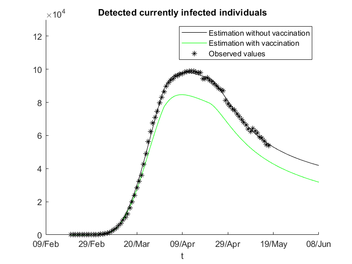
Figure 1: Detected currently infected individuals (Spain)

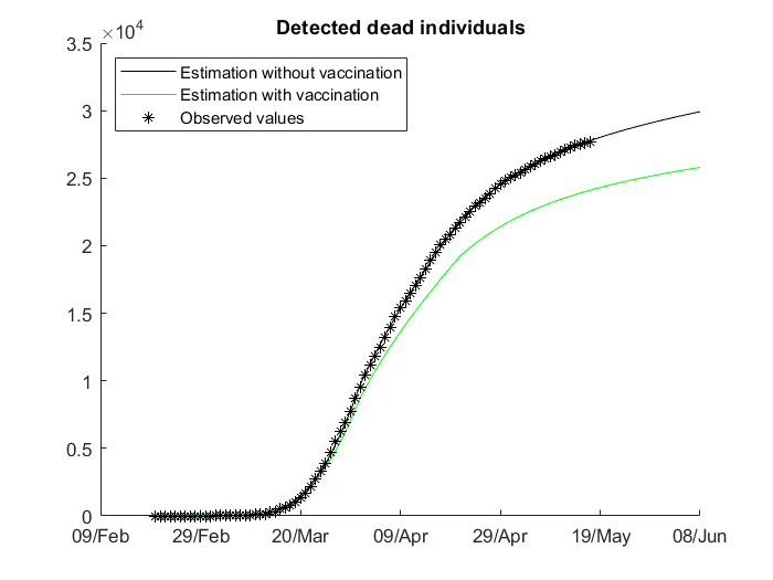
Figure 2: Detected dead individuals (Spain)

6 Application to the COVID-19 spread in the Valencian region

In this section, we will study the effect of an hypothetical vacunation during the first wave of the COVID-19 pandemic in the Spanish region called Valencian Community.

Again, we choose an average value for $\rho$ given by the study of seroprevalence in Spain Instituto de Salud Carlos III, (2020). According to it, at the end of May of 2020 2,8% of the population of the valencian region had been infected by the virus (which gives about 140,000 infected people as the population is 5 millions), whereas an approximate number of 11,000 people were detected by the COVID tests at that moment. Thus, the average rate of detection during the first wave of the pandemic in the valencian region was approximately equal to $0.08$.

As before, we set $\sigma=1/5.$

We estimate the parameters of the model in the period from February 25, 2020 to May 12, 2020, splitting this interval into the following five subintervals: 1) 25/02-13/03; 2) 13/03-31/03; 3) 31/03-8/04; 4) 8/04-5/05; 5) 5/05-12/05.

We proceed in the same way as in the previous section. In this case, on the 25th of February the number of detected detected active infected individuals was $1$, so the estimate of the real number of infected subjects is $1/\rho=13$, whereas the number of dead and recovered people, as in the case of Spain, are equal to $0$. Hence, the initial conditions are the following

$$I_{0}=13\text{, }F_{0}=0,\ R_{0}=0,\ L_{0}=0,\ S_{0}=N-I_{0}-E_{0}-F_{0}-R_{0}-L_{0}.$$

The estimate of the parameters in each interval is the following:

1. 25/02-13/03: $\beta\left(t\right)=\beta_{0}=0.45327,\ \gamma_{1}\left(t\right)=\gamma_{0,1}=0.0047971,\ \gamma_{2}\left(t\right)=\gamma_{0,2}=0.0035465,\ E_{0}=122.25849.$

2. 13/03-31/03: $\beta\left(t\right)=2.42072-2.29381\left(1-e^{-0.29565\left(t-17\right)}\right),$ $\gamma_{1}\left(t\right)=0.016886-0.015126(1-e^{-0.048468(t-17)}),$ $\gamma_{2}\left(t\right)=0.0014814+0.028856(1-e^{-0.014266(t-17)}).$

3. 31/03-8/04: $\beta\left(t\right)=7.20401\ast 10^{-7}-6.86704\ast 10^{-7}(1-e^{-29439.63489(t-35)}),$ $\gamma_{1}(t)=0.017352-0.010442(1-e^{-0.78599(t-35)}),$ $\gamma_{2}\left(t\right)=0.29292-0.26096(1-e^{-8.41998(t-35)}).$

4. 8/04-5/05: $\beta\left(t\right)=0.39963-0.38539(1-e^{-2.72216(t-43)}),$ $\gamma_{1}\left(t\right)=0.0023469+0.003184(1-e^{-1.3958(t-43)}),$ $\gamma_{2}\left(t\right)=0.033247+0.045749(1-e^{-0.11634(t-43)}).$

5. 5/05-12/05: $\beta\left(t\right)=\beta_{0}=1.834401-1.834398(1-e^{-30.03165(t-70)}),$ $\gamma_{1}(t)=0.0014464+0.02423(1-e^{-0.14298(t-70)}),$ $\gamma_{2}\left(t\right)=1.92157\ast 10^{-5}+0.34632(1-e^{-1.18519(t-70)}).$

We proceed in the same way as in the previous section by solving system (5) with a constant number of vaccinated people per day in each period. Also, the distribution of the vaccines will be exactly the same, varying only the number $\Delta$.

In the following table we can see the predictions of the model concerning detected deaths at the end of the whole period (i.e. on the 12-th of May) and detected infected people at the peak of the pandemic (i.e. on the 5-th of April) with two values of the variable $\Delta$:

	Deaths	Infections
Observed values	$1341$	$5767$
$\Delta=10000$	$1214$	$5237$
$\Delta=20000$	$1102$	$4747$

In Figures 3, 4 we can see the evolution of the number of detected dead people and detected infected people with and without vaccination in the case where $\Delta=20000$.

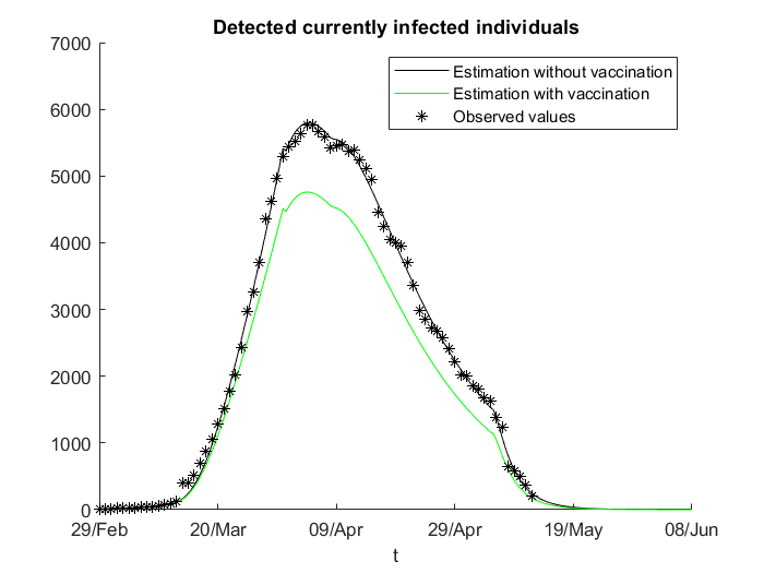
Figure 3: Detected currently infected individuals (Valencian Community)

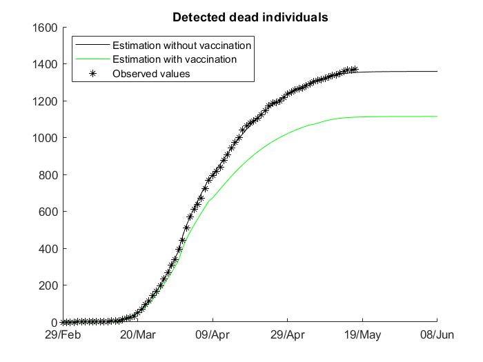
Figure 4: Detected dead individuals (Valencian Community)

7 Optimal distribution approach

The aim of the distribution method is to schedule the distribution of vaccines among the locations of a region over time within a temporal horizon but according to the established priority groups. So, even though the space-time component is added, no one will be vaccinated until all people belonging to the highest priority groups have been vaccinated regardless of their location. The addition of the spatio-temporal component is motivated by minimizing the total number of infected cases in the region during the considered temporal horizon. In other words, our objective is to maximize the number of saved infected cases. We note that the saved infected cases are not only the vaccinated people but also the people that could be infected by them in case of contracting the disease if they were not vaccinated. Then, if we distribute the same number of vaccines in two locations at the same instant of time, the total number of saved infected cases due to this distribution will be different.

The distribution method is based on forecasting the number of infected people which would be saved by vaccinating one person in one location from the first shot to the end of the period. Then, at each instant, as many doses as possible are assigned to the most advantageous location. However, there are other aspects that complicate the algorithm like vaccination by priority groups, the application of a second dose after a while, etc.

1 estimate parameters and state variables for $l$ from $data$ until $t-1$

2 $\bar{p}=$ forecasting of infected cases at $T$ without vaccination

3 $p=$ forecasting of infected cases at $T$ with $\Delta_{1}(t)=1$

return $\bar{p}-p$

Algorithm 2 gain($t$, $l$,$data$)

Algorithm 2 forecasts infection savings due to the application of the first shot to one person at location $l$ and instant $t$. Using the estimation of parameters from the observed data without vaccination and the applied vaccines until the moment of time $t-1$, we solve system (5) and simulate new observed values of our variables by taking into account the chosen hypothetical vaccination in this period. After that, with these new observed data, we estimate again the parameters of the system until the moment $t-1$ using Algorithm 1, because we need to perform now the estimation using the observed data that have been simulated taking into account vaccination. Then we solve first system (5) until the end of the period $T$ with none vaccination, forecasting $\bar{p}$ infected cases, and after that we solve systeml (5) with $\Delta_{1}(t)=1$, forecasting $p$ infected cases. We note that the day of the application of first doses can be chosen, but not the day of the application of the second ones. Then, the difference $\bar{p}-p$ estimates the number of infection savings at location $l$ for the rest of the period due to the assignation of one vaccine to location $l$ at instant $t$.

1 for each $s\in rows(S)$ do

2       if $S[s,2]+\delta=t$ then

3             $d_{S[s,0],S[s,1],2}=S[s,3]$

4             $\#vaccines=\#vaccines-S[s,3]$

5             delete $S[s,\cdot]$

6            

7      

8 while $\#vaccines>0$ do

9       $l^{*}=$ location with maximum value of $gain(t,l,data)$ $\forall l\in L$ such that $r_{l^{*},g}>0$

10       $d_{l^{*},g,1}=min\{r_{l^{*},g},\#vaccines\}$

11       $m=rows(S)+1$

12       $S[m,0]=l^{*}$; $S[m,1]=g$; $S[m,2]=t$; $S[m,3]=d_{l^{*},g,1}$;

13       $\#vaccines=\#vaccines-d_{l^{*},g,1}$

14       $r_{l^{*},g}=r_{l^{*},g}-d_{l^{*},g,1}$

15       if $r_{l,g}=0,$ $\forall l\in L$ then $g=g+1$

16      

return $D$

Algorithm 3 optimal_distribution($t$, $g$, $\#vaccines$, $data$)

Algorithm 3 returns the optimal matrix distribution $D=\{d_{l,g,i}\}$ which indicates the number of vaccines that will be distributed at the current instant $t$ for each location $l$ and group $g$. The subindex $i$ is equal to $1$ if we use our method of distribution of vaccines and equal to $2$ if we use a random distribution. Its input parameters are the current instant $t$, the target priority group $g$, the number of vaccines $\#vaccines$ to be assigned at instant $t$ and the historical data of the pandemic spread.

Since $\delta$ days after the first we must assign a second dose to the people vaccinated once, this algorithm manages a list that contains the number of first doses which have been already applied, in which location, to which group and at what time. That is the purpose of the list $S,$ representing its column $S[\cdot,0]$ the location in which a first vaccination has been carried out, whereas $S[\cdot,1]$ shows to which priority group, $S[\cdot,2]$ contains the data of this first vaccination and $S[\cdot,3]$ contains the number of vaccinated people. On the other hand, the matrix $\{r_{l,g}\}$ saves the number of unvaccinated people belonging to each location $l$ and priority each group $g$.

First of all, the vaccines are assigned to the people for whom their second vaccination deadline is $t$. We note that if the number of vaccines to be applied every day is constant, or at least the second doses are reserved, the distribution to this people is assured. Lines 3 to 3 describe this procedure. We go through the rows of list $S$ in order to locate which people are at the deadline date, that is, for each row $s$ such that $S[s,2]+\delta=t$, $S[s,3]$ vaccines are assigned to the group $S[s,1]$ and location $S[s,0]$ as second dose. Besides, the number of vaccines employed is subtracted from the remaining amount, and since these people are fully vaccinated, this row is removed from the list. If the number of diary disposable vaccines is constant, according to this procedure, a period of $\delta$ days where exclusively first doses are applied is followed by a period of $\delta$ days where exclusively second shots are applied.

In the rest of the algorithm first doses are distributed in order to achieve the greatest effectiveness. At the current instant $t$, we find the location $l^{\ast}$ with the highest profit after applying one first shot and such that there are some unvaccinated people belonging to the group $g$, that is, $r_{l^{\ast},g}>0$. Hence, we will schedule as many doses as possible to location $l^{\ast}$ and group $g$.

On the one hand, lines 3 - 3 of Algorithm 3 show how to assign as many first doses as possible. The minimum number between the vaccines available and the people of location $l^{\ast}$ and group $g$ pending for the first vaccination constitutes the maximum number of vaccines to be assigned to group $g$ and location $l^{\ast}$, so $d_{l^{\ast},g,1}=min\{r_{l^{\ast},g},\#vaccines\}$. Since these vaccinated people will require a second dose, we have to add a new row to the list $S$. This is done using the following lines of code, in which we add one row and write in its cells the values of the location, the group, the instant and the number of vaccines distributed. Finally, we have to subtract this number from the number of available vaccines and from the number of unvaccinated people. If all the people of group $g$ have already been vaccinated at all the locations then we move on to the next target group.

We also point out that, although it has only been shown how to obtain the distribution of vaccines for instant $t,$ if obtaining a schedule in advance for more instants is required, this can be obtained by successive projections doing $t=t+1$ and calling Algorithm 3 again.

8 Computational experience

In this section, we will analyse the computational results of the proposed distribution approach, comparing it with the random selection of individuals to be vaccinated regardless of their location, but both according to the established priority groups. First, we will explain the algorithm which is used to simulate the number of infections, detected cases, deaths and immunity level applying both distributions. Secondly, we will describe how the priority groups were parametrized as well as the different instances that were simulated. Finally, we will report the obtained results.

Algorithm 4 shows the procedure which is used in order to simulate the number of infections, detected cases, deaths and immunity level applying both distributions. Then we estimate all the parameters and state variables for the entire analysed period. We also set the initial instant $t_{0}$ at which the analysed period begins and we assign the priority group to $1$.

1 $\rho$ = estimate of parameters from the historical data

2 $t=t_{0}$

3 $g_{p}=1$

4 $data_{opt},data_{ran}$=historical data until $t_{0}-1$

5 while $t<|T|$ do

6       $O=optimal\_distribution(t,g_{p},\#vaccines,data_{opt})$

7       $R=$ random distribution of $\#vaccines$ between priority groups

8       $data_{opt}(t)$=simulation of data from $\rho$ at $t$ applying $O$

9       $data_{prop}(t)$=simulation of data from $\rho$ at $t$ applying $R$

10       $t=t+1$

11      

return $\#Infections(data_{prop})$ - $\#Infections(data_{opt})$

Algorithm 4 simulation

Since in reality there has been no vaccination during the analysed period, it is necessary to introduce two serial of data to simulate the effect of the two vaccine distributions for this period. Serial $data_{opt}$ will contain the simulated infections, deaths and distributed vaccines when we distribute the vaccines according to our approach. Serial $data_{ran}$ will be simulated by distributing the available vaccines every day randomly selecting the individuals of each group regardless of their location. These vaccines will be assigned first to people with second dose deadline and the remaining to people belonging to the priority group. Once everyone belonging to the priority group has received their first dose then we move on to the next priority group. Note that both serials are broken down by date and location in the same format as the historical data. Until the instant $t_{0}-1$ both lists are equal to the historical data.

Lines 4 to 4 constitute a loop in which the period is successively traversed obtaining for each instant two vaccine distributions: the distribution using our approach $O$ and the random distribution $R$. After that, for each instant the effect of both vaccine distributions is simulated, obtaining new infections and deaths for each location according to each distribution. We note that $data_{opt}$ and $data_{prop}$ are obtained applying model (5) with the parameters being estimated in the model without vaccination using the historical observed data. However, each time procedure gain is called from $optimal\_distribution$ a new estimate of all the parameters is carried out, as shown before in Algorithm 2. All the simulations are done using system (5) with constant coefficients.

As the conditions and parameters are different according to different circumstances as the lockdown phases, the use of masks, etc. the parameters are defined and estimated piecewise for each week. This is similar to what is done in Sections 5, 6 but now the intervals are chosen in periods of seven days because in this way it can be automatically fixed, avoiding thus the need to define the intervals depending on the government restrictions as lockdown or curfew.

Regarding the settings of the Differential Evolution technique which have been used in this application, a population of $N=100$ individuals has been established. The coefficients $K,F\in(0,1]$ were randomly generated at each iteration. Finally, the estimation is stopped when a maximum number of $10000$ iterations is achieved.

We have applied our method to the pandemic spread in the Spanish region called Valencian Community during the period from the 1st of Juny to the 31th of December of 2020. The data on detected infections and deaths have been collected from GVA, (2020). They are disaggregated by date and town. As it is said, our approach adds the spatio-temporal component to the priority group that has been established by the authorities. At this respect, in our computational experience, we have supposed for each group the priority and proportions which are indicated in Table 1.

Priority	Group	Population	Proportion
1	Residents of nursing homes and health workers	50,573	$2.00\%$
2	Over 90 years of age	49,307	$0.97\%$
3	People from 80 to 89 years of age	227,224	$4.49\%$
4	People from 70 to 79 years of age	437,862	$8.66\%$
5	People from 60 to 69 years of age	580,728	$11.48\%$
6	People from 50 to 59 years of age	752,334	$14.88\%$
7	People from 40 to 49 years of age	851,588	$16.84\%$
8	People from 30 to 39 years of age	648,759	$12.83\%$
9	People from 20 to 29 years of age	516,126	$10.21\%$
10	People from 12 to 19 years of age	424,531	$8.39\%$

Table 1: Priorities, size and proportions of each group

Table 1 indicates that people over 90 years of age cannot be vaccinated until residents of nursing homes and health workders have been vaccinated, people from 80 to 89 years of age cannot be vaccinated until residents of nursing homes and health workers and people over 90 have been vaccinated, and so on. But the decision maker has to choose the people to be vaccinated as long as they belong to the target group. Or more exactly, for the purposes of our study, the decision maker can choose the population of those who belong to the target group. Table 1 also shows the size and the proportion of each group. The proportion of residents of nursing homes and health workers has simply been assumed. However, the rest of sizes and percentages have been extracted from Instituto Nacional de Estadística, (2020). Children under 12 years of age are not considered to be vaccinated, being 5,057,353 the size of the entire population including them. Figure 5 shows the population pyramide of Valencian Community. For simplicity, we consider that these population proportions are identical for each town, which is clearly not a true fact. In practice, if they were known, they could be adjusted differently for each town. Nevertheless, setting identical proportions regardless of the place also constitutes a way for carrying out fair and equitable distributions among the populations, which is another of the principles exposed in EUCommission, 2020a .

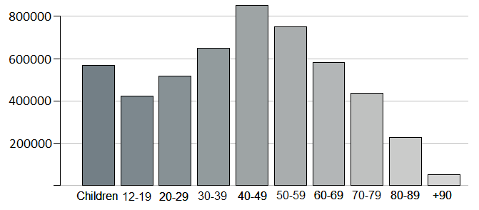
Figure 5: Population pyramid of Valencian Community

BNT162b2 is assumed to be the vaccine used for all injections. Its first dose reaches an effectiveness of 54% and, after the application of the second shot 21 days later, an effectiveness of 95%. These percentages and the recommended period between shots have been established according to Tartof et al., (2020). Regarding the recommended period, this has been strictly assumed, which means that a second shot is applied to each vaccinated person exactly 21 days after the first one.

In addition, to get a wide computational experience, we have prepared several examples with different number of distributed doses and percentage of people willing to be vaccinated. These instances are:

• one case in which no vaccine is shot;

• eleven cases with 10, 25, 50, 75, 100, 250, 500, 750, 1,000 thousands of doses;

We note that 1 million doses means that approximately 500 thousands people receive their full vaccination program. The reasons for analysing up to 1,000 thousand doses are as follows:

• these quantities of doses are feasible to apply in the period studied;

• a higher number than 1,000 thousand doses would imply an homogeneous distribution, even when attempting to prioritize the populations with higher impact, as it would require extrem mass distribution;

• the simplification that has been proposed for the probability of being susceptible (that is, $S(t)/N$) is valid for these quantities.

Table 2 summarizes the obtained results relative to the infected cases. Doses indentifies the case, Random and Approach show the estimated infected cases by using the random distribution and our approach, R. Saving and A. Saving contain the number of saved infections with both methods and, finally, Column Advantage shows the difference A. Saving minus R. Saving.

Doses	Random	Approach	R. Saving	A. Saving	Advantage
10,000	261,254	260,519	150	885	735
25,000	260,856	259,778	548	1,626	1,078
50,000	260,145	258,852	1,259	2,552	1,293
75,000	259,831	258,289	1,573	3,115	1,542
100,000	258,561	256,699	2,843	4,705	1,862
250,000	255,907	248,866	5,497	12,538	7,041
500,000	250,999	240,930	10,405	20,474	10,069
750,000	243,438	230,571	17,966	30,833	12,867
1,000,000	239,819	226,398	21,585	35,006	13,421

Table 2: Infected cases by both distribution methods

The number of infected people was estimated to be equal to $261,404$ in the studied period without vaccination. Hence, both saving columns are calculated by substracting from $261,404$ the estimated values by each method. Besides, these values are also represented in Figure 6 and Column Advantage. Finally, Figure 7 shows the difference between them. In both methods, it can also be seen that the more vaccines the less infected people and, therefore, the case in which $1$ million doses are applied is the more effective to slow down the pandemic. Besides, the proposed method always improves the random distribution.

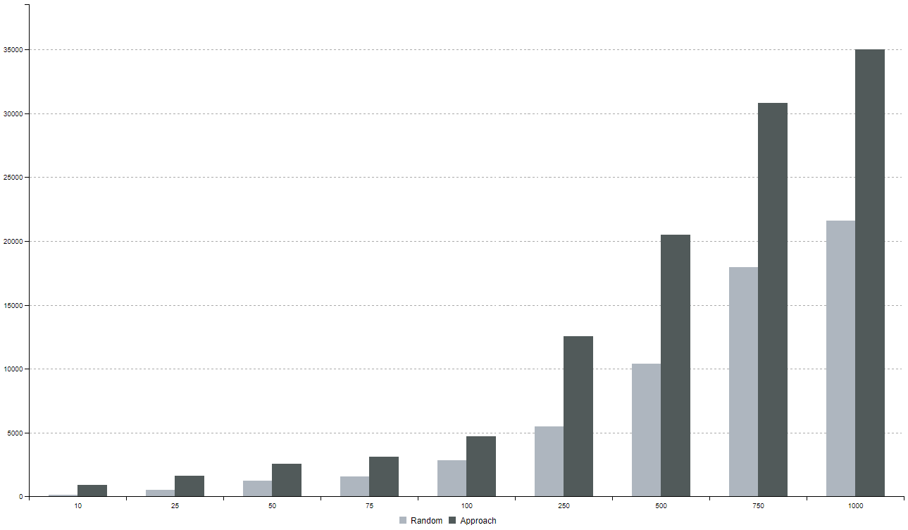
Figure 6: Infected cases by both distribution methods

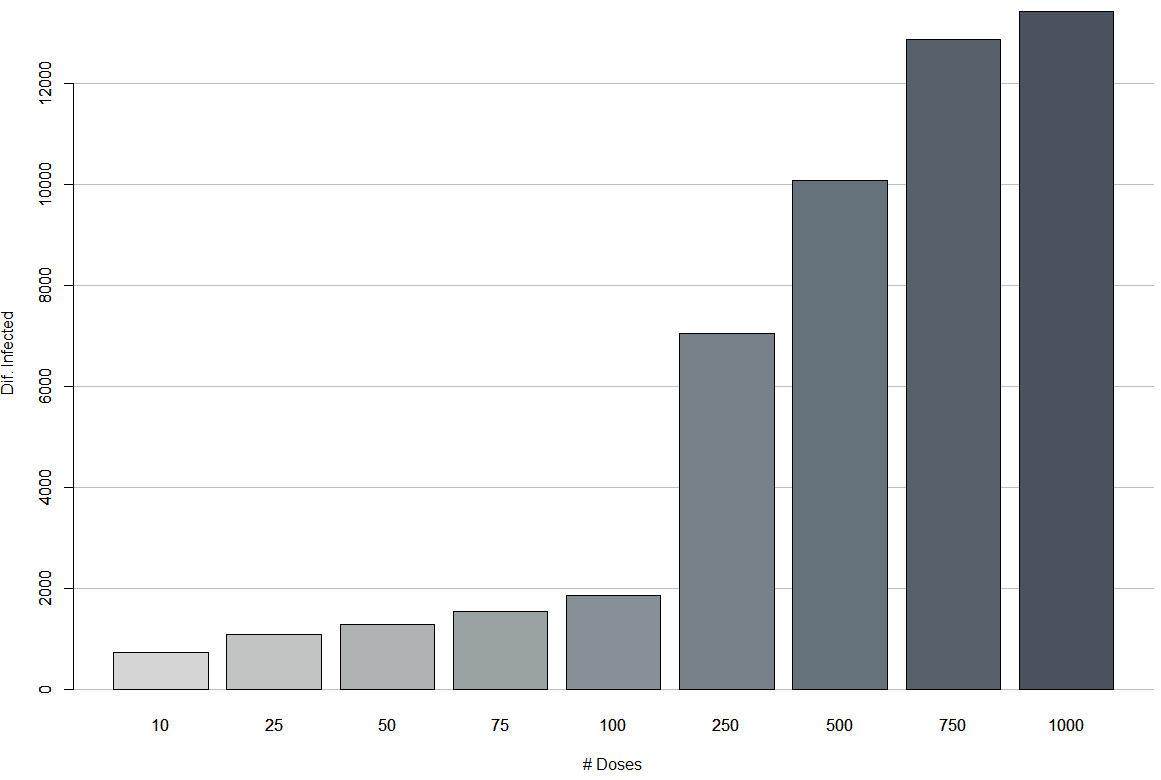
Figure 7: Difference of infected cases by both distribution methods

Table 3 and figures 8 and 9 are relative to the number of detected cases in the simulations. They are equivalent to the already commented table and figures of the infected cases and the savings are calculated from the estimation of $149,754$ detected cases for the period without vaccination. Regarding them, the results, figures and conclusions are similar to those of the infected cases. Then, the proposed method always improves the random distribution.

Doses	Random	Approach	R. Saving	A. Saving	Advantage
10,000	148,997	148,660	757	1,094	337
25,000	148,800	148,262	954	1,492	538
50,000	148,419	147,745	1,335	2,009	674
75,000	148,312	147,452	1,442	2,302	860
100,000	147,625	146,724	2,129	3,030	901
250,000	146,295	142,480	3,459	7,274	3,815
500,000	143,801	138,331	5,953	11,423	5,470
750,000	140,403	132,664	9,351	17,090	7,739
1,000,000	138,312	130,446	11,442	19,308	7,866

Table 3: Detected cases by both distribution methods

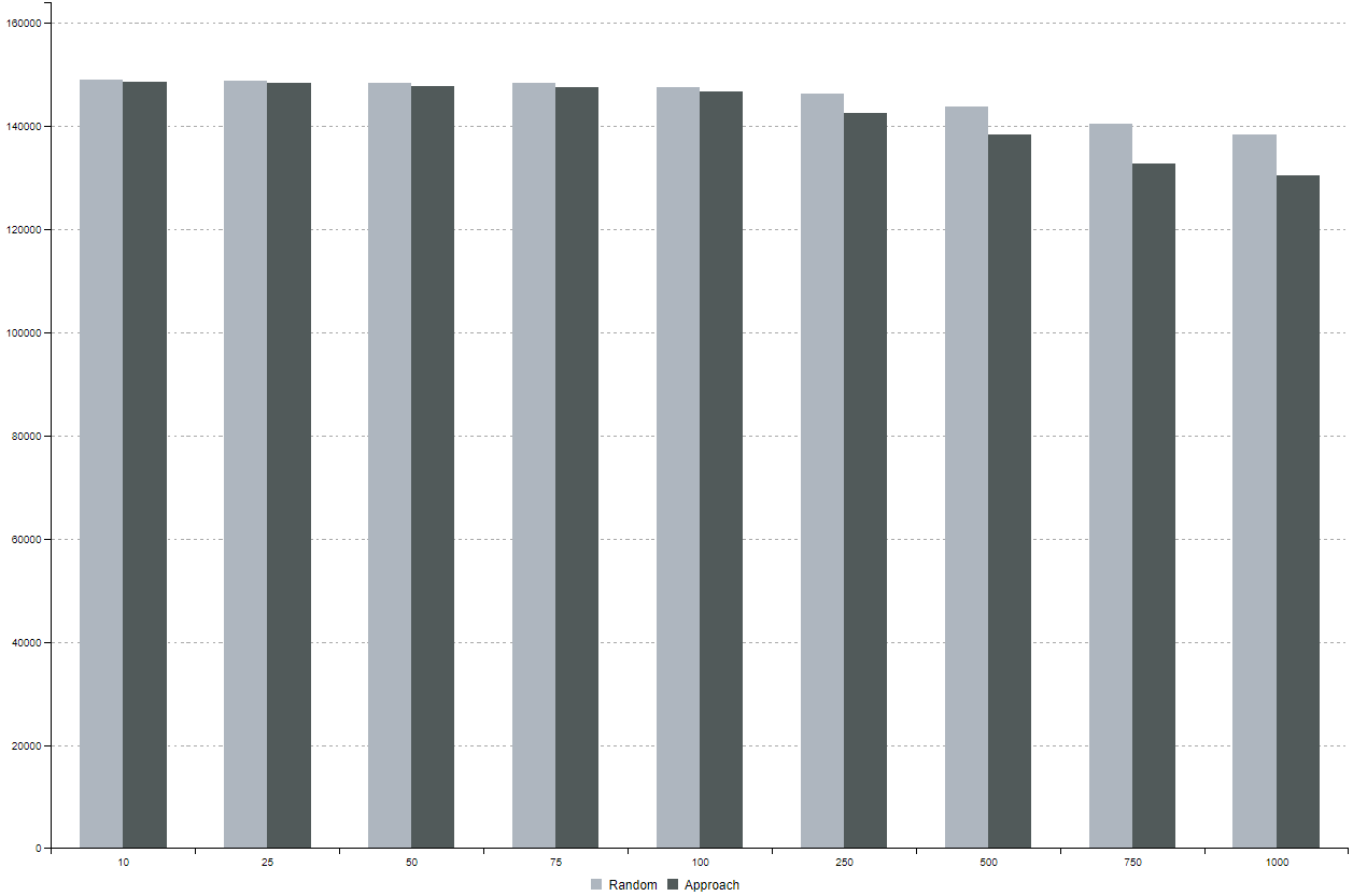
Figure 8: Detected cases by both distribution methods

Figure 9: Difference of detected cases by both distribution methods

Table 4 summarizes the obtained results relative to the number of detected deaths, and its columns and interpretation are the same as in the previous tables. We remember that model (5) only offers measures about deaths that can be detected. 4,001 detected deaths are estimated in the period without vaccination. Then, the estimated deaths are subtracted from this value in order to get both savings. Again, as it can be guessed, the more vaccines given, the lower the number of deaths. Besides, the proposed approach is more advantageous in general, although the random distribution has slightly better values in three cases with negative advantage, despite the fact that the number of infections is always lower when our approach is used. In this regard, it is necessary to note that the main objective of this method is to reduce the number of infections and, as a side effect, also the number of deaths; but the latter is not its priority.

Doses	Random	Approach	R. Saving	A. Saving	Advantage
10,000	4,000	3,993	1	8	7
25,000	3,998	3,971	3	30	27
50,000	3,964	3,966	37	35	-2
75,000	3,978	3,940	23	61	38
100,000	3,912	3,932	89	69	-20
250,000	3,914	3,824	87	177	90
500,000	3,531	3,556	470	445	-25
750,000	3,779	3,531	222	470	248
1,000,000	3,643	3,583	358	418	60

Table 4: Number of detected deaths by both distribution methods

Figures 10 and 11 illustrate, respectively, the number of deaths by both methods and its difference.

Figure 10: Detected deaths by both distribution methods

Figure 11: Difference of detected deaths by both distribution methods

Finally, Table 5 reports the percentage of population immunity achieved by both methods. Obviously, the more vaccination the higher percentage of immunity. It can be observed that both methods present similar values for the number of doses that are simulated, getting a percentage higher than 9 % of immunity when $1$ million vaccines are used. However, random distribution provides a slightly higher immunisation. The explanation of this is due to the fact that more people are infected if random distribution is used. Therefore, it is natural immunisation that contributes to this difference.

Doses	Random	Approach
10,000	8,4746 %	8,4631 %
25,000	8,4841 %	8,4675 %
50,000	8,5083 %	8,4806 %
75,000	8,5360 %	8,5034 %
10,0000	8,5489 %	8,5133 %
25,0000	8,6997 %	8,5632 %
500,000	9,0051 %	8,7607 %
750,000	9,2016 %	8,9051 %
100,0000	9,6375 %	9,1243 %

Table 5: Percentages of immunization by both distribution methods

9 Conclusions

In this work, a SEIR model for analysing the efficiency of vaccine distributions has been introduced. This model takes into account the presence of both detected and non-detected infected individuals as well as the lockdown of detected cases and, of course, vaccination. Since the values of the parameters of the model can change abruptly due to severe governments measures like lockdown, curfew, etc., the coefficients of the model are defined piecewise in given intervals of time and are functions of time. This model has been applied to the spread of the COVID pandemic in Spain and the Spanish region called Valencian Community. Besides, some theoretical results concerning convergence of solutions in the lon term and stability of stationary points haven been proved.

On the other hand, we describe the Differential Evolution technique, which is a genetic algorithm for the estimation of parameters, and develop a heuristic approach for optimising the distribution of vaccines in order to minimize the number of infected cases. This approach have been applied to the spreading of COVID-19 pandemic in the Valencian Community by an extensive computational experience showing the advantages of the proposed distribution method.

Acknowledgments

This work has been partially supported by the Generalitat Valenciana (Spain), project CIGE/2021/161. The first author has also been partially supported by the Spanish Ministry of Science, Innovation and Universities, project PID2021-122344NB-I00. The second author has also been partially supported by the Spanish Ministry of Science and Innovation, projects PID2019-108654GB-I00 and PDI2021-122991NB-C21.

References

- Bai et al., (2021) Bai, N., Song, C., and Xu, R. (2021). Mathematical analysis and application of a cholera transmission model with waning vaccine-induced immunity. Nonlinear Analysis: Real World Applications, 58.
- Brauer and Castillo-Chávez, (2012) Brauer, F. and Castillo-Chávez, C. (2012). Mathematical models in population biology and epidemiology. Springer, New-York.
- Chauhan et al., (2014) Chauhan, S., Misra, O., and Dhar, J. (2014). Stability analysis of SIR model with vaccination. American Journal of Computational and Applied Mathematics, 4:17–23.
- (4) EUCommission (2020a). Coronavirus: Commission lists key steps for effective vaccination strategies and vaccines deployment. Press corner: https://ec.europa.eu/commission/presscorner/detail/en/ip_20_1903.
- (5) EUCommission (2020b). Preparedness for COVID-19 vaccination strategies and vaccine deployment. Communication from the commission to the European parliament and the council.
- Gutierrez and Varona, (2020) Gutierrez, J. and Varona, J. (2020). Analisis de la posible evolución de la epidemia de coronavirus COVID-19 por medio de un modelo SEIR https://belenus.unirioja.es/jvarona/coronavirus/SEIR-coronavirus.pdf.
- GVA, (2020) GVA (2020). Valencian community, COVID-19 confirmed cases: http://www.pegv.gva.es/en/dbcv. Valencian Community opden data.
- Instituto de Salud Carlos III, (2020) Instituto de Salud Carlos III (2020). Estudio ENE-COVID: Informe final. estudio nacional de sero-epidemiología de la infección por SARS-COV-2 en españa: https://portalcne.isciii.es/enecovid19. Estudio Nacional de sero-epidemiología de la infección por SARS-COV-2 en España.
- Instituto Nacional de Estadística, (2020) Instituto Nacional de Estadística (2020). Población por comunidades, edad (grupos quinquenales), españoles/extranjeros, sexo y año: https://www.ine.es/dynt3/inebase/es/index.htm?type=pcaxis&path=/t20/e245/p08/&file=pcaxis&dh=0&capsel=1. Base de datos del Instituto Nacional de Estadística.
- Iorio and Li, (2006) Iorio, A. and Li, X. (2006). Incorporating directional information within a differential evolution algorithm for multi-objective optimization. Proceeding of the Genetic and Evolutionary Computation Conference 2006, pages 691–697.
- Kotyrba et al., (2015) Kotyrba, M., Volna, E., and Bujok, P. (2015). Unconventional modelling of complex system via cellular automata and differential evolution. Swarm and Evolutionary Computation, 25:52–62.
- Kribs-Zaleta and Velasco-Hernández, (2000) Kribs-Zaleta, C. and Velasco-Hernández, J. (2000). A simple vaccination model with multiple endemic states. Mathematical Biosciences, 164:183–201.
- Lauer et al., (2019) Lauer, S., Grantz, K., Q. Bi, F. J., Zheng, Q., and Meredith, H. (2019). The incubation period of coronavirus disease 2019 (COVID-19) from publicly reported confirmed cases: Estimation and application. Ann. Intern. Med., 172:577–582.
- Li and Muldowney, (1995) Li, M. and Muldowney, J. (1995). Global stability for the seir model in epidemiology. Mathematical Biosciencies, 125:155–164.
- Li and Wang, (2001) Li, M. and Wang, L. (2001). Global stability in some seir epidemic model. In Mathematical Approaches for Emerging and Reemerging Infectious Diseases Part II: Models, Methods and Theory (Castillo-Chavez et al., eds.), volume 126 of IMA Volumes in Mathematics and its Applications, pages 295–311. Springer-Verlag.
- Li et al., (2020) Li, R., Pei, S., Chen, B., Song, Y., Zhangf, T., Yang, W., and Shaman, J. (2020). Substantial undocumented infection facilitates the rapid dissemination of novel coronavirus (SARS-CoV-2). Science, 368:489–493.
- Lin et al., (2020) Lin, Q., Zhao, S., Gao, D., Lou, Y., Yang, S., Musa, S., Wang, M., Cai, Y., Wang, W., Yang, L., and He, D. (2020). A conceptual model for the coronavirus disease 2019 (COVID-19) outbreak in wuhan, china with individual reaction and governmental action. International Journal of Infectious Diseases, 93:211–216.
- Rai et al., (2022) Rai, B., Shukla, A., and Dwivedi, L. (2022). Incubation period for COVID-19: a systematic review and meta-analysis. J. Public Health: From Theory to Practice, 30:2649–2656.
- Sainz-Pardo and Valero, (2021) Sainz-Pardo, J. and Valero, J. (2021). COVID-19 and other viruses: Holding back its spreading by massive testing. Expert Systems with Applications, 186.
- Storn, (1996) Storn, R. (1996). On the usage of differential evolution for function optimization. Proceedings of the 1996 Biennial Conference of the North American Fuzzy Information Processing Society, pages 519–523.
- Tang et al., (2020) Tang, B., Bragazzi, N., Li, Q., Tang, S., Xiao, Y., and J. Wu, A. (2020). Updated estimation of the risk of transmission of the novel coronavirus (2019-ncov). Infectious Disease Modelling, 5:248–255.
- Tartof et al., (2020) Tartof, S., Slezak, J., Fischer, H., Hong, V., Ackerson, B., Ranasinghe, O., Frankland, T., Ogun, O., Zamparo, J., and Gray, S. (2020). Effectiveness of MRNA BNT162b2 COVID-19 vaccine up to 6 months in a large integrated health system in the usa: A retrospective cohort study. Lancet, 398:1407–1416.
- Wangari, (2020) Wangari, I. (2020). Condition for global stability for a seir model incorporating exogenous reinfection and primary infection mechanisms. Computational and Mathematical Methods in Medicine, 2020:Article ID 9435819.
- Wei and Xue, (2020) Wei, F. and Xue, R. (2020). Stability and extinction of SEIR epidemic models with generalized nonlinear incidence. Mathematics and Computers in Simulation, 170:1–15.
- Wiggins, (2003) Wiggins, S. (2003). Introduction to applied nonlinear dynamical systems and chaos. Springer, New-York.
- Xua et al., (2010) Xua, R., Mab, Z., and Wanga, Z. (2010). Global stability of a delayed SIRS epidemic model with saturation incidence and temporary immunity. Computers and Mathematics with Applications, 59:3211–3221.
- Xue, (2022) Xue, C. (2022). Study on the global stability for a generalized SEIR epidemic model. Computational Intelligence and Neuroscience, 2022:Article ID 8215214.
- Zhao et al., (2017) Zhao, Y., Jiang, D., and O’Regan, D. (2017). The extinction and persistence of the stochastic SIS epidemic model with vaccination. Physica A: Statistical Mechanics and its Applications, 392:4916–4927.