Meta Co-Training: Two Views are Better than One

Abstract

In many practical computer vision scenarios unlabeled data is plentiful, but labels are scarce and difficult to obtain. As a result, semi-supervised learning which leverages unlabeled data to boost the performance of supervised classifiers have received significant attention in recent literature. One major class of semi-supervised algorithms is co-training. In co-training two different models leverage different independent and sufficient “views” of the data to jointly make better predictions. During co-training each model creates pseudo labels on unlabeled points which are used to improve the other model. We show that in the common case when independent views are not available we can construct such views inexpensively using pre-trained models. Co-training on the constructed views yields a performance improvement over any of the individual views we construct and performance comparable with recent approaches in semi-supervised learning, but has some undesirable properties. To alleviate the issues present with co-training we present Meta Co-Training which is an extension of the successful Meta Pseudo Labels approach to two views. Our method achieves new state-of-the-art performance on ImageNet-10% with very few training resources, as well as outperforming prior semi-supervised work on several other fine-grained image classification datasets.

1 Introduction

In many practical machine learning scenarios we have access to a large amount of unlabeled data, and relatively few labeled data points for the task on which we would like to train. For generic computer vision (CV) tasks there are large well-known and open source datasets with hundreds of millions or even billions of unlabeled images [62, 63]. In contrast, labeled data is usually scarce and expensive to obtain requiring many human-hours to generate. Hence, in this context, semi-supervised learning (SSL) methods are becoming increasingly popular as they rely on training useful learning models by using small amounts of labeled data and large amounts of unlabeled data.

Not unrelated to, and not to be confused with the idea of semi-supervised learning, is self-supervised learning. In self-supervised learning a model is trained with an objective that does not require a label that is not evident from the data itself. Self-supervised learning was popularized by the BERT [32] model for generating word embeddings for natural language processing (NLP) tasks. BERT generates its embeddings by solving the pretext task of masked word prediction. Pretext tasks present unsupervised objectives that are not directly related to any particular supervised objective we might desire to solve, but rather are solved in the hope of learning a suitable representation to more easily solve a downstream task. Due to the foundational nature of these models to the success of many models in NLP, or perhaps the fact that they serve as a foundation for other models to be built upon, these pretext learners are often referred to as foundation models. Inspired by foundation models from NLP, several pretext tasks have been proposed for CV with associated foundation models that have been trained to solve them [8, 38, 20, 42, 23, 49, 19, 58, 24, 43]. Unlike NLP, the learned representations for images are often much smaller than the images themselves which yields the additional benefit of reduced computational effort when using the learned representations.

Typically, SSL requires the learner to make predictions on a large amount of unlabeled data as well as the labeled data during training. Furthermore, SSL often requires that the learner be re-trained [12, 76, 50, 72, 48, 55, 39, 70, 74, 40, 17] partially, or from scratch. Given the computational benefits of learning from a frozen representation, combining SSL and self-supervised learning is a natural idea. Additionally, the representation learner allows us to compress our data to a smaller size. This compression is beneficial not only because of the reduction in operations required that is associated with a smaller model, but also because it allows us to occupy less space on disk, in RAM, and in high bandwidth memory on hardware accelerators.

These benefits are particularly pronounced for co-training [12] in which two different “views” of the data must be obtained or constructed and then two different classifiers must be trained and re-trained iteratively. Seldom does a standard problem in machine learning present two independent and sufficient views of the problem to be leveraged for co-training. As a result, if one hopes to apply co-training one usually needs to construct two views from the view that they have. To take advantage of the computational advantages of representation learning, and the large body of self-supervised literature, we propose using the embeddings produced by foundation models trained on different pretext tasks as the views for co-training. To our knowledge we are the first to propose using frozen learned feature representations as views for co-training classification, though we think the idea is very natural. We show that views constructed in this way appear to satisfy the necessary conditions for the effectiveness of co-training.

Unfortunately, while we can boost performance by training different models on two views, co-training performs sub-optimally during its pseudo-labeling step. To more effectively leverage two views we propose a novel method for co-training based on Meta Pseudo Labels [59] called Meta Co-Training in which each model is trained to provide better pseudo labels to the other given only its view of the labeled data and the performance of the other model on the labeled set. We show that our approach provides an improvement over both co-training and the current state-of-the-art (SotA) on the ImageNet-10% dataset, as well as it establishes new SotA few-shot performance on several other fine-grained image classification tasks.

Summary of Contributions.   Our contributions are therefore summarized as follows.

1. Use of embeddings obtained from different pre-trained models as different views for co-training.

2. We boost the performance of standard co-training by proposing a method that relies on Meta Pseudo Labels [59], called Meta Co-Training.

3. We establish new state-of-the-art top-1 accuracy on ImageNet-10% [31] and new state-of-the-art top-1 few-shot accuracy on several other CV classification tasks.

4. We make our implementation publicly available:
   https://github.com/JayRothenberger/Meta-Co-Training

Outline of the Paper.   In Section 2 we discuss related work. In Section 3 we establish notation and provide more information on co-training and meta pseudo labels. In Section 4 we describe our proposed methods of view construction and of meta co-training. In Section 5 we present and discuss our experimental findings on ImageNet [31], Flowers102 [57], Food101 [14], FGVCAircraft [54], iNaturalist [44], and iNaturalist 2021 [45]. In Section 6 we conclude with a summary and ideas for future work.

2 Related Work

While SSL [21, 78, 67, 73] has become very relevant in recent years with the influx of the data collected by various sensors, the paradigm and its usefulness have been studied at least since the 1960’s; e.g., [41, 29, 64, 36]. Among the main approaches for SSL that are not directly related to our work, we find techniques that try to identify the maximum likelihood parameters for mixture models [30, 7], constrained clustering [9, 28, 69, 68, 18, 3], graph-based methods [11, 10, 53, 6], as well as purely theoretical probably approximately correct (PAC)-style results [4, 37, 25]. Below we discuss SSL approaches closer to our work.

Self-Training and Student-Teacher Frameworks.   One of the earliest ideas for SSL is that of self-training [64, 36]. This idea is still very popular with different student-teacher frameworks [79, 76, 59, 50, 72, 66, 55, 39, 17]. This technique is also frequently referred to as pseudo-labeling [48] as the student tries to improve its performance by making predictions on the unlabeled data, then integrating the most confident predictions to the labeled set, and subsequently retraining using the broader labeled set. In addition, one can combine ideas; e.g., self-training with clustering [46], or create ensembles via self-training [47], potentially using graph-based information [53]. An issue with these approaches is that of confirmation bias [2], where the student cannot improve a lot due to incorrect labeling that occurs either because of self-training, or due to a fallible teacher.

Co-Training.   Another paradigmatic family of SSL algorithms are co-training [12] algorithms, where instances have two different views for the same underlying phenomenon. Co-training has been very successful with wide applicability [34] and can outperform learning algorithms that use only single-view data [56]. Furthermore, the generalization ability of co-training is well-motivated theoretically [12, 27, 5, 26]. There are several natural extensions of the base idea, such as methods for constructing different views [71, 15, 22, 65, 16], including connections to active learning [33], methods that are specific to deep learning [60], and other natural extensions that exploit more than two views on data; e.g., [77].

3 Background

We briefly describe two important components of semi-supervised learning that are used jointly in order to devise our proposed new technique. However, before we do so, we also define basic notions so that we can eliminate ambiguity.

3.1 Notation

Supervised learning is based on the idea of learning a function, called a model, $f$ belonging to some model space $\mathcal{F}$, using training examples $(x,y)$ that exemplify some underlying phenomenon. Training examples are labeled instances; i.e., $x\in\mathcal{X}$ is an instance drawn from some instance space $\mathcal{X}$ and $y$ is a label from some label set $\mathcal{Y}$. This relationship between $\mathcal{X}$ and $\mathcal{Y}$ can be modeled with a probability distribution $D$ that governs $\mathcal{X}\times\mathcal{Y}$. We write $(x,y)\sim D$ to indicate that a training example $(x,y)$ is drawn from $\mathcal{X}\times\mathcal{Y}$ according to $D$. We use $\mathbf{1}\left\{\mathcal{A}\right\}$ as an indicator function of the event $\mathcal{A}$; that is, $\mathbf{1}\left\{\mathcal{A}\right\}$ is equal to 1 when $\mathcal{A}$ holds, otherwise 0. For vectors $\alpha,\beta\in\mathbb{R}^{d}$ we indicate their Hadamard (element-wise) product using $\otimes$; that is, $\gamma=\alpha\otimes\beta$, where $\gamma_{j}=\alpha_{j}\cdot\beta_{j}$ for $j\in\{1,\ldots,d\}$.

As is standard in classification problems, we let model $f$ be a function of the form $f\colon\mathcal{X}\rightarrow\Delta^{|\mathcal{Y}|}$ where $\Delta^{|\mathcal{Y}|}$ is the $|\mathcal{Y}|$-dimensional unit simplex. Equivalently $f$ can be understood as a probability distribution $\mathbf{Pr}(y\ |\ x)$. We use $f(x)|_{j}$ to denote the $j$-th value of $f$ in the output in such a case. It is common for $\mathcal{F}$ to be a parameterized family of functions (e.g. artificial neural networks). We use $\theta$ as a vector that holds such parameters, and we denote the function parameterized by $\theta$ as $f_{\theta}$. An individual prediction $f_{\theta}(x)$ for an instance $x$ is evaluated via the use of a loss function $\ell$ that determines the quality of the prediction $f_{\theta}(x)$ with respect to the actual value $y$ that should have been predicted. For classification problems a natural way of defining loss functions is of the form $\ell\colon\mathcal{Y}\times\Delta^{|\mathcal{Y}|}\rightarrow\mathbb{R}_{+}$. For the entirety of this text $\ell$ will refer to the cross-entropy loss which is defined as $\ell\left(y,f_{\theta}(x)\right)=-\sum_{\xi\in\mathcal{Y}}\mathbf{1}\left\{\xi=y\right\}\log\left(f_{\theta}(x)|_{\xi}\right)$.

We measure the performance of a model $f_{\theta}$ by its (true) risk $R_{D}\left(f_{\theta}\right)=\mathbf{E}_{(x,y)\sim D}\left[\ell\left(y,f_{\theta}(x)\right)\right]$. While we want to create a model $f_{\theta}$ that has low true risk, in principle we apply empirical risk minimization (ERM) which yields a model $f_{\theta}$ that minimizes the risk over a set of training examples. That is, we use empirical risk as a proxy for the true risk. Given a set $S=\left\{(x_{i},y_{i})\right\}_{i=1}^{\left\lvert S\right\rvert}$, we denote the empirical risk of $f_{\theta}$ on $S$ as $\widehat{R}_{S}\left(f_{\theta}\right)=\frac{1}{\left\lvert S\right\rvert}\sum_{i=1}^{\left\lvert S\right\rvert}\ell\left(y,f_{\theta}(x)\right)$. To ease notation, when the inputs to $\ell$ are a batch of examples $(X,Y)$, we denote $\widehat{R}_{(X,Y)}\left(f_{\theta}\right)$ as simply $\ell(Y,f_{\theta}(X))$. Similarly, when we write the arg max of a batch of vectors we refer to the batch of the arg max of the individual values. In general, ERM can be computationally hard (e.g., [13, 1]); hence, we often rely on gradient-based optimization techniques, such as stochastic gradient descent (SGD), that can take us to a local optimum efficiently. We use $\eta$ as the learning rate and $T$ as the maximum number of steps (or updates) in such a gradient-based optimization procedure.

Semi-Supervised Learning.   We are interested in situations where we have a large pool of unlabeled instances $U$ as well as a small portion $L$ of them that is labeled. That is, the learning algorithm has access to a dataset $S=L\cup U$, such that $L=\left\{(x_{i},y_{i})\right\}_{i=1}^{m}$ and $U=\left\{x_{j}\right\}_{j=1}^{u}$. In this setting, semi-supervised learning (SSL) methods attempt to first learn an initial model $f_{init}$ using the labeled data $L$ via a supervised learning algorithm, and in sequence, an attempt is being made in order to harness the information that is hidden in the unlabeled set $U$, so that a better model $f$ can be learnt.

3.2 Meta Pseudo Labels

In order to discuss Meta Pseudo Labels, first we need to discuss Pseudo Labels. Pseudo Labels (PL) [48] is a broad paradigm for SSL, which involves a teacher and a student in the learning process. The teacher looking at the unlabeled set $U$, selects a few instances and assigns pseudo-labels to them. Subsequently these pseudo-examples are shown to the student as if they were legitimate examples so that the student can learn a better model. In this context, the teacher $f_{\theta_{T}}$ is fixed and the student is trying to learn a better model by aligning its predictions to pseudo-labeled batches $(X_{u},f_{\theta_{T}}(X_{u}))$. Thus, on a pseudo-labeled batch, the student optimizes its parameters using

$$\theta_{S}^{\text{PL}}\in\operatorname*{arg\,min}_{\theta_{S}}\ell\left(\operatorname*{arg\,max}_{\xi}f_{\theta_{T}}(X_{u})|_{\xi},f_{\theta_{S}}(X_{u})\right)\,.$$ (1)

The hope is that updated student parameters $\theta_{S}^{\text{PL}}$ will behave well on the labeled data $L=(X_{L},Y_{L})=\left\{(x_{i},y_{i})\right\}_{i=1}^{m}$; that is, the loss $\mathcal{L}_{L}\left(\theta_{S}^{\text{PL}}\left(\theta_{T}\right)\right)=\ell\left(Y_{L},f_{\theta_{S}^{\text{PL}}}(X_{L})\right)$ is small, where $\mathcal{L}\left(\theta_{S}^{\text{PL}}\left(\theta_{T}\right)\right)$ is defined so that the dependence between $\theta_{S}$ and $\theta_{T}$ is explicit.

Meta Pseudo Labels (MPL) [59] is exploiting this dependence between $\theta_{S}$ and $\theta_{T}$. In other words, because the loss that the student suffers on $\mathcal{L}_{L}\left(\theta_{S}^{\text{PL}}\left(\theta_{T}\right)\right)$ is a function of $\theta_{T}$, and making a similar notational convention for the unlabeled batch $\mathcal{L}_{u}\left(\theta_{T},\theta_{S}\right)=\ell\left(\operatorname*{arg\,max}_{\xi}f_{\theta_{T}}(X_{u})|_{\xi},f_{\theta_{S}}(X_{u})\right)$, then one can further optimize $\theta_{T}$ as a function of the performance of $\theta_{S}$:

$$\left\{\begin{array}[]{rl}\displaystyle\min_{\theta_{T}}&\displaystyle\mathcal{L}_{L}\left(\theta_{S}^{\text{PL}}\left(\theta_{T}\right)\right)\,,\\[3.00003pt] \text{where}&\displaystyle\theta_{S}^{\text{PL}}(\theta_{T})\in\operatorname*{arg\,min}_{\theta_{S}}\mathcal{L}_{u}\left(\theta_{T},\theta_{S}\right)\,.\end{array}\right.$$ (2)

However, because the dependency between $\theta_{T}$ and $\theta_{S}$ is complicated, a practical approximation [51, 35] is obtained via $\theta_{S}^{\text{PL}}\approx\theta_{S}-\eta_{S}\cdot\nabla_{\theta_{S}}\mathcal{L}_{u}\left(\theta_{T},\theta_{S}\right)$ which leads to the practical teacher objective:

$$\min_{\theta_{T}}\mathcal{L}_{L}\left(\theta_{S}-\eta_{S}\cdot\nabla_{\theta_{S}}\mathcal{L}_{u}\left(\theta_{T},\theta_{S}\right)\right)\,.$$ (3)

For more information the interested reader can refer to [59].

3.3 Co-Training

Co-training relies on the existence of two different views of the instance space $\mathcal{X}$; that is, $\mathcal{X}=\mathcal{X}^{(1)}\times\mathcal{X}^{(2)}$. Hence, an instance $x\in\mathcal{X}$ has the form $x=(x^{(1)},x^{(2)})\in\mathcal{X}^{(1)}\times\mathcal{X}^{(2)}$. We say that the views $x^{(1)}$ and $x^{(2)}$ are complementary. Co-training requires two assumptions in order to work. First, it is assumed that, provided enough many examples, each separate view is enough for learning a meaningful model. The second is the conditional independence assumption [12], which states that $x^{(1)}$ and $x^{(2)}$ are conditionally independent given the label of the instance $x=(x^{(1)},x^{(2)})$. Thus, with co-training, two models $f^{(1)}$ and $f^{(2)}$ are learnt, which help each other using different information that they capture from the different views of each instance. More information is presented below.

Given a dataset $S=L\cup U$ (Section 3.1 has notation), we can have access to two different views of the dataset due to the natural partitioning of the instance space $\mathcal{X}$; that is, $S^{(1)}=L^{(1)}\cup U^{(1)}$ and $S^{(2)}=L^{(2)}\cup U^{(2)}$. Initially two models $f^{(1)}$ and $f^{(2)}$ are learnt using a supervised learning algorithm based on the labeled sets $L^{(1)}$ and $L^{(2)}$ respectively. Learning proceeds in iterations, where in each iteration a number of unlabeled instances are integrated with the labeled set by assigning pseudo-labels to them that are predicted by $f^{(1)}$ and $f^{(2)}$, so that improved models $f^{(1)}$ and $f^{(2)}$ can be learnt by retraining on the augmented labeled sets. In particular, in each iteration, each model $f^{(v)}$ predicts a label for each view $x^{(v)}\in U^{(v)}$. The top-$k$ most confident predictions by model $f^{(v)}$ are used to provide a pseudo label for the respective complementary instances and then these pseudo-labeled examples are integrated in to the labeled set for the complementary view. In the next iteration a new model is trained based on the augmented labeled set. Both views of the used instances are dropped from $U$ even if only one of the views may be used for augmenting the appropriate labeled set. This process repeats until the unlabeled sets $U^{(v)}$ are exhausted, yielding models $f^{(1)}$ and $f^{(2)}$ corresponding to the two views. Co-Training is evaluated using the joint prediction of these models which is the re-normalized element-wise product of the two predictions:

$$\frac{f^{(1)}\left(x^{(1)}\right)\otimes f^{(2)}\left(x^{(2)}\right)}{\left\lVert f^{(1)}\left(x^{(1)}\right)\otimes f^{(2)}\left(x^{(2)}\right)\right\rVert_{1}}\,.$$ (4)

Co-training was introduced by Blum and Mitchell [12] and their paradigmatic example was classifying web pages using two different views: (i) the bags of words based on the content that they had and (ii) the bag of words formed by the words that were used for hyperlinks pointing to these webpages. In our context the two different views are obtained via different embeddings that we obtain when we use images as inputs to different foundation models and observe the resulting embeddings.

4 Proposed Methods

4.1 View Construction

Past methods of view construction include manual feature subsetting [33], automatic feature subsetting [22, 65],

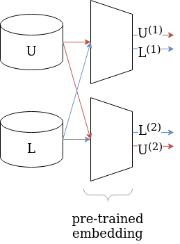
Figure 1: Using pre-trained models for constructing views.

random feature subsetting [15, 16], random subspace selection [16], and adversarial examples [60]. We propose a method of view construction which is motivated by modern approaches to SSL and representation learning in computer vision and natural language processing: pretext learning.

Given two pretext tasks we can train a model to accomplish each task, then use their learned embedding spaces as separate views for classification. If we have chosen our pretext tasks well, then the representations will be different, compressed, and capture sufficient information to perform the desired downstream task. Figure 1 demonstrates the idea of the method. Even if one does not have access to different views on a particular dataset, the use of different pre-trained models allows the creation of different views; as the transformation happens at the level of instances, it applies to both labeled and unlabeled batches alike as shown in Figure 1 with $L$ and $U$ respectively. However, if one has access to a dataset where the instances have two different views, then one can still obtain useful representations with this approach using even the same pre-trained model. Furthermore, one can also use multiple pre-trained models and concatenate the resulting embeddings so that two separate views with richer information content can be created and are still low-dimensional.

While our approach is more widely applicable, it is particularly well-suited to computer vision. There are a plethora [38, 23, 24, 19, 49, 20, 61, 58, 42] of competitive learned representations for images. Recently it has been popular to treat these representations as task-agnostic foundation models. We show that the existence of these models eliminates the need to train new models for pretext tasks to achieve state-of-the-art performance for SSL-classification. Furthermore, it is comparatively very cheap to use the foundation models instead as not only can we forego training on a pretext task, but we are able to completely bypass the need to train a large convolutional neural network (CNN) or vision transformer (ViT). In fact, we compute the embedding for each of the images in our dataset only one time (as opposed to applying some form of data augmentation during training and making use of the embedding process during training). So, at training time the only weights we need to use at all are those in the model we train on top of the learned representation. This makes our approach incredibly lightweight compared to traditional CNN/ViT training procedures.

4.2 Meta Co-Training

In addition to our method of view construction we propose a novel algorithm for co-training which is based on Meta Pseudo Labels [59], called Meta Co-Training (MCT), which is described below.

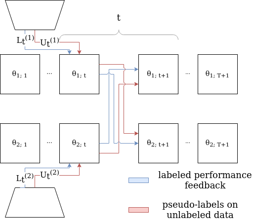
Figure 2: At each step $t\in\{1,\ldots,T\}$ of meta co-training the models that correspond to the so-far learnt parameters $\theta_{1;t}$ and $\theta_{2;t}$ play the role of the student and the teacher simultaneously using batches for their respective views. Pseudo-labeling occurs on complementary views so that the teacher can provide the student with labels on an unlabeled batch. Labeled batches may, or may not, use complementary views as the purpose that they serve is to calculate the risk of the student model on the labeled batch and this result signals the teacher model to update its weights accordingly.

1:  Input: $L^{(1)},L^{(2)},U^{(1)},U^{(2)},f^{(1)},f^{(2)},\theta_{1},\theta_{2},T,\ell,\eta$

2:  for step $t\in\{1\dots T\}$ do

3:     // Unlabeled views must be complementary

4:     $U_{t}^{(1)}\leftarrow SampleBatch(U^{(1)})$

5:     $U_{t}^{(2)}\leftarrow getOtherView(U_{t}^{(1)},2)$

6:     // Predict soft pseudo labels

7:     $\hat{y}^{(1)}\leftarrow f^{(1)}_{\theta_{1}}(U_{t}^{(1)})$

8:     $\hat{y}^{(2)}\leftarrow f^{(2)}_{\theta_{2}}(U_{t}^{(2)})$

9:     // Sample the pseudo labels from the discrete distribution over the classes

10:     $PL^{(1)}\sim\hat{y}^{(1)}$

11:     $PL^{(2)}\sim\hat{y}^{(2)}$

12:     // MPL student update applied to both models

13:     $\theta^{\prime}_{1}\leftarrow\theta_{1}-\eta\cdot\nabla_{\theta_{1}}\ell(PL^{(2)},\hat{y}^{(1)})$

14:     $\theta^{\prime}_{2}\leftarrow\theta_{2}-\eta\cdot\nabla_{\theta_{2}}\ell(PL^{(1)},\hat{y}^{(2)})$

15:     // Sample batches from $L$ for the teacher updates

16:     $X_{t}^{(1)},Y_{t}^{(1)}\leftarrow SampleBatch(L^{(1)})$

17:     $X_{t}^{(2)},Y_{t}^{(2)}\leftarrow SampleBatch(L^{(2)})$

18:     // MPL teacher update applied to both models

19:     $\hat{y}^{\prime(1)}\leftarrow f^{(1)}_{\theta^{\prime}_{1}}(X_{t}^{(1)})$

20:     $\hat{y}^{\prime(2)}\leftarrow f^{(2)}_{\theta^{\prime}_{2}}(X_{t}^{(2)})$

21:     $h^{(1)}\leftarrow\nabla_{\theta^{\prime}_{2}}\ell(Y_{t}^{(2)},\hat{y}^{\prime(2)})^{T}\cdot\nabla_{\theta_{2}}\ell(PL^{(1)},\hat{y}^{(2)})$

22:     $h^{(2)}\leftarrow\nabla_{\theta^{\prime}_{1}}\ell(Y_{t}^{(1)},\hat{y}^{\prime(1)})^{T}\cdot\nabla_{\theta_{1}}\ell(PL^{(2)},\hat{y}^{(1)})$

23:     // Weights to be used in the next step

24:     $\theta_{1}\leftarrow\theta^{\prime}_{1}-\eta\cdot h^{(1)}\cdot\nabla_{\theta_{1}}\ell(PL^{(1)},\hat{y}^{(1)})$

25:     $\theta_{2}\leftarrow\theta^{\prime}_{2}-\eta\cdot h^{(2)}\cdot\nabla_{\theta_{2}}\ell(PL^{(2)},\hat{y}^{(2)})$

26:  end for

Algorithm 1 Meta Co-Training (Section 3.1 has notation)

4.2.1 Overview of Meta Co-Training (MCT)

An overview of MCT is provided in Figure 2. At each step $t\in\{1,\ldots,T\}$ of meta co-training the models that correspond to the so-far learnt parameters $\theta_{1;t}$ and $\theta_{2;t}$ play the role of the student and the teacher simultaneously on batches from their respective views. The (low-dimensional) embeddings obtained from the view construction process of Section 4.1 form different views that are used by MCT.

When a student model predicts labels on an unlabeled batch it suffers loss based on the pseudo-labels that are provided by the teacher model (which uses the complementary view for the unlabeled instances) and the student weights are adjusted accordingly. Then the student model evaluates the performance of its new weights on separate labeled batches. This performance provides feedback to the teacher model. Geometrically, we can understand this as updating the parameters in the direction of increasing confidence on our pseudo labels if those labels helped the other model perform better on the labeled set, or in the opposite direction if it hurt the other model’s performance on the labeled set.

Finally, similar to MPL, we assume that at $t=1$ models have been pre-trained using supervised warmup period so that their predictions are not random. This is analogous to the fully-supervised iteration of co-training.

4.2.2 Algorithmic Details

Algorithm 1 presents the details in pseudocode. The function SampleBatch, is sampling a batch from the dataset. The function getOtherView returns the complementary view of the first argument; the second argument clarifies which view should be returned (“2” in line 5). At each step $t$ of the algorithm each model is first updated based on the pseudo labels the other has provided on a batch of unlabeled data (Lines 13-14). Then each model is updated to provide labels that encourage the other to predict more correctly on the labeled set based on the performance of the other (Lines 24-25). We refer the reader to Section 3.2 (resp. [59]) for a brief (resp. complete) discussion of the MPL approach. Note that contrary to traditional co-training, no new pseudo-labeled data are added to the labeled set, neither are any data removed from the unlabeled set after each step.

5 Experimental Evaluation

Towards evaluating the proposed method of view construction for co-training we first constructed views of the data utilizing five different learned representations. Our primary comparisons were on the widely-used ImageNet [31] classification task; however, Sections 5.4 and B provide experimental results on additional image classification tasks. To produce the views used to train the classifiers during co-training and meta co-training we used the embedding space of five representation learning architectures: The Masked Autoencoder (MAE) [42], DINOv2 [58], SwAV [19], EsViT [49], and CLIP [61]. We selected the models which produce the views as they have been learned in an unsupervised way, have been made available by the authors of their respective papers for use in PyTorch, and have been shown to produce representations that are appropriate for ImageNet classification.

5.1 Investigating the Co-Training Assumptions on the Constructed Views

Motivated by the analysis and experiments of [34] we made an effort to verify the sufficiency and independence of the representations learned by the aforementioned models.

On the Sufficiency of the Views.   Sufficiency is fairly easy to verify. If we choose a reasonable sufficiency threshold for the task, for ImageNet say close or above $70\%$ top-1 accuracy, then we can train simple models on the views of the dataset we have constructed and provide examples of functions which demonstrate the satisfaction of the property. We tested a single linear layer with softmax output, as well as a simple 3-layer multi-layer perceptron (MLP) with 1024 neurons per layer and dense skip connections (previous layer outputs were concatenated to input for subsequent layers) to provide a lower bound on the sufficiency of the views on the standard subsets of the ImageNet labels for semi-supervised classification.

Model	1%	10%	100%
MAE	1.9	3.2	73.5
DINOv2	78.1	82.9	86.3
SwAV	12.1	41.1	77.9
EsViT	69.1	74.4	81.3
CLIP	74.1	80.9	85.4

Table 1: Linear probe evaluation for views. Top-1 accuracy on different subsets of the ImageNet data are shown.

Model	1%	10%
MAE	23.4	48.5
DINOv2	78.4	82.7
SwAV	12.5	32.6
EsViT	71.3	75.8
CLIP	75.2	80.9

Table 2: MLP performance on individual views. Top-1 accuracy on different subsets of the ImageNet data are shown.

From these experiments, whose results are shown in Tables 1 and 2 resepectively, we can see that if we were to pick a threshold for top-1 accuracy around $70\%$, which we believe indicates considerable skill without presenting too high of a bar, then EsViT, CLIP, and DINOv2 provide sufficient views for both the $1\%$ and $10\%$ subsets.

On the Independence of the Views.   To test the independence of the views generated by the representation learning models, we trained an identical MLP architecture to predict each view from each other view; Table 3 presents our findings, explained below.

	MAE	DINOv2	SwAV	EsViT	CLIP
MAE	-	0.139	0.142	0.137	0.129
DINOv2	0.110	-	0.132	0.135	0.130
SwAV	0.116	0.147	-	0.137	0.126
EsViT	0.112	0.140	0.116	-	0.135
CLIP	0.110	0.146	0.136	0.156	-

Table 3: Pairwise translation performance of linear probe on the ImageNet dataset. A linear classifier is trained on the output of an MLP which is trained to predict one view (columns) from another view (rows) by minimizing MSE. The top-1 accuracy (%) of the linear classifier is reported. Both the MLP and the linear classifier have access to the entire embedded ImageNet training set.

Given as input the view to predict from (rows of Table 3) the MLPs were trained to reduce the mean squared error (MSE) between their output and the view to be predicted (columns of Table 3). We then trained a linear classifier on the outputs generated by the MLP given every training set embedding from each view. Had the model faithfully reconstructed the output view given only the input view then we would expect the linear classifier to perform similarly to the last column of Table 1. The linear classifiers never did much better than a random guess on the ImageNet class achieving at most 0.156% accuracy. Thus, while we cannot immediately conclude that the views are independent, it is clearly not trivial to predict one view given any other. We believe that this is compelling evidence for the independence of different representations.

5.2 Experimental Evaluation on ImageNet

Having constructed at least two strong views of the data, and suspecting that these views are independent we hypothesize that co-training will work on this data. In Table 4(a) we show the results of applying the standard co-training algorithm [12].

	DINOv2	SwAV	EsViT	CLIP
MAE	81.8 (75.5)	30.5 (11.4)	77.1 (66.2)	78.8 (66.8)
DINOv2		78.5 (74.5)	83.3 (78.9)	85.1 (80.1)
SwAV			70.6 ( 64.9)	75.5 (67.4)
EsViT				82.3 ( 76.9)

(a) Co-Training

	DINOv2	SwAV	EsViT	CLIP
MAE	81.2 (73.8)	37.6 (8.1)	73.6 ( 63.8)	78.6 (63.5)
DINOv2		77.3 ( 70.7)	83.4 (79.2)	85.2 (80.7)
SwAV			74.4 (67.3)	77.1 (67.4)
EsViT				82.4 (77.5)

(b) Meta Co-Training

Table 4: Co-training and meta co-training top-1 accuracy of view combinations on 10% (1%) of ImageNet labels. As co-training does not depend on the order of the views, we show only upper-diagonal entries of the pairwise comparison. Diagonal entries would correspond to views which are trivially dependent. All $\binom{5}{2}=10$ different combinations of views are shown in each table.

At each iteration of co-training the model made a prediction for all of the instances in $U$, following (4). We assigned labels to the 10% of the total original unlabeled data with most confident predictions for both models. When confident predictions conflicted on examples, we returned those instances to the unlabeled set, otherwise they entered the labeled set of the other model with the assigned pseudo-label.

Predicting according to (4) yielded better accuracy than the predictions of each individual model. In addition, in our experiments on ImageNet, as co-training iterations proceeded top-1 accuracy decreased. Later we show that this was not always the case (see Figure 11 in the appendix). The decrease was less pronounced when the views perform at a similar level; see Figure 3.

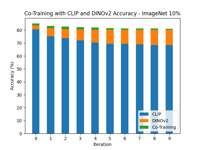
Figure 3: Top-1 accuracy of co-training iterations on the CLIP and DINOv2 views for the ImageNet 10% dataset.

However, meta co-training does not exhibit performance degradation - in fact this is an ideal case where the method performs best; see Figure 4.

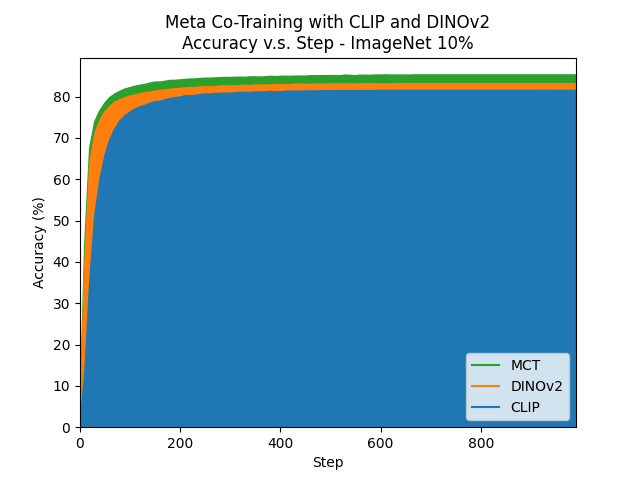
Figure 4: Meta co-training using the CLIP and DINOv2 views as a function of the training step. Models are trained on 10% of the ImageNet labels.

While Figures 3 and 4 correspond to ImageNet 10%, similar observations also hold for ImageNet 1%; please see the appendix.

Comparing co-training accuracy on ImageNet 10% (resp. 1%) shown in Table 4(a) compared to MLP accuracy shown in Table 2, we observe that co-training top-1 accuracy is on average 18.7% (resp. 16.8%) higher than MLP accuracy. Moreover, the best co-training top-1 accuracy is 2.4% (resp. 1.7%) higher compared to the best top-1 MLP accuracy. In other words, co-training resulted in a significant increase in prediction accuracy but not after the warmup iteration finished. Meta co-training, however, continues to improve after the warmup period has elapsed. See Figures 5 and 6 for a comparison in the case of ImageNet 10%; a similar comparison for ImageNet 1% is presented in the appendix.

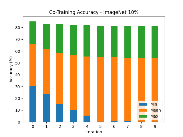
Figure 5: Top-1 accuracy of co-training iterations for the ImageNet 10% dataset. The average over all 10 pairs, the best pair, and the worst pair at each iteration are shown.

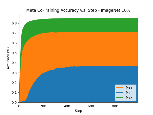
Figure 6: Aggregate statistics of meta co-training across all views. Models are trained on 10% of the ImageNet labels. The maximum performance of any pair, the minimum performance of any pair, and the average of all 10 pairs is shown.

Despite the poor performance of the pseudo-labeling during co-training, using the two best performing views in (4) performed as well as the previous SotA method for semi-supervised classification on the ImageNet-10%; see Co-Training in Table 5. The performance of co-training as a method was rather disappointing in that the algorithm is unable to leverage pseudo-labels to improve the accuracy on this task; however, the results do show that our view-construction method has merit. Given the difficulty of translating between the views, and the fact that the accuracy yielded by (4) is greater than its constituent views, we believe the poor performance of the pseudo-labeling step in co-training was due to low information content of at least one view rather than view-dependence.

Reference	Model	Method	ImageNet-1%	ImageNet-10%
[49]	EsViT (Swin-B, W=14)	Linear	69.1	74.4
[42]	MAE (ViT-L)	MLP	23.4	48.5
[61]	CLIP (ViT-L)	Fine-tuned	80.5	84.7
[58]	DINOv2 (ViT-L)	Linear	78.1	82.9
[24]	SimCLRv2 (ResNet152-w2)	Fine-tuned	74.2	79.4
[19]	SwAV (RN50-w4)	Fine-tuned	53.9	70.2
[60]	Deep Co-Training (ResNet-18)	Co-Training	-	53.5
[17]	Semi-ViT (ViT-L)	Self-trained	77.3	83.3
[52]	REACT (ViT-L)	REACT	81.6	85.1
[59]	MPL (EfficientNet-B6-Wide)	MPL	-	73.9
[12]	Co-Training (MLP)*	Co-Training	80.1	85.1
	MCT (MLP)* - ours	MCT	80.7	85.8

Table 5: Performance of different approaches on ImageNet dataset. An asterisk (*) indicates models that were trained on top of embeddings generated by much larger models. During training we do not need to alter the parameters of these larger models, and these larger models need not see data used for downstream classification during their training, however training of downstream models would not have been possible without the embeddings. Models on the lower half of the table use unlabeled data during classification training.

5.2.1 More on Meta Co-Training

To draw fair comparisons we fix the model architecture and view set from our experiments on co-training. As in MPL [59] a supervised loss is optimized jointly with a loss on pseudo-labels. Like MPL, we found that beginning with a warmup period in which the model trained in a strictly supervised way expedited training. This warmup period occurs for the same number of updates as the first training phase of co-training, so each method starts with the same number of supervised updates before pseudo-labeling. Unlike MPL, we did not use Unsupervised Data Augmentation [75], because we embedded the dataset only once, and due to the nature of the pretext tasks that were used to generate the views we did not believe data augmentation would have much of an effect. Details of our training recipe appear in Table 10.

Comparing the top-1 accuracy of MCT and co-training on ImageNet 10% (resp. 1%) shown in Table 5, we observe that MCTyielded a difference on average 0.7% (resp. -0.6%) compared to co-training. Moreover, MCT top-1 accuracy is 0.1% (resp. 0.6%) higher overall. Note that on all view pairs in which co-training beats MCT, apart from the $10\%$ (EsViT, MAE) pair, one of the views alone was better than co-training. The single DINOv2 view outperforms all such view pairs. These are all cases in which one of the views was significantly weaker than the other. For the experiments in which we had two strong (e.g., not SwAV or MAE) views, MCT always performed better than co-training.

5.3 Stronger Views by Concatenation

Finally, we take the four views which had the greatest performance and constructed two views out of them by concatenating them together. We constructed one view CLIP $|$ EsViT and the second DINOv2 $|$ SwAV and measured the performance of co-training and meta co-training on these views in Table 6. Interestingly, co-training does not benefit from these larger views; see Table 6.

Method	1%	10%
Co-Training	80.0	84.8
MCT	80.5	85.8

Table 6: Co-training and MCT evaluated on the ImageNet dataset using the CLIP $|$ EsViT and DINOv2 $|$ SwAV views.

The additional information may have allowed the individual models to overfit their training data quickly. During meta co-training we observed that after one model reaches 100% training accuracy, its validation accuracy can still improve by learning to label for the other model. Possibly due to the rapid overfitting due to the increased view size (and consequently increased parameter count) the 1% split did not show improvement for either model.

	Dataset
Method	Flowers102	Food101	FGVCAircraft
REACT (ViT-L)	97.0	85.6	57.1
Co-Training (MLP)	99.2	94.7	36.4
MCT (MLP)	99.6	94.8	40.1

Table 7: Additional Comparisons to REACT [52]. The authors include experiments for zero-shot performance and 10% of available labels. Results above are for 10% of labels. For Flowers102 this is 1-shot performance.

	Dataset
Method	iNaturalist	Food101
Semi-ViT (ViT-B)	67.7 (32.3)	84.5 (60.9)
Co-Training (MLP)	59.7 (29.5)	94.7 (83.9)
MCT (MLP)	76.0 (58.1)	94.8 (91.7)

Table 8: Additional Comparisons to Semi-ViT using 10% (1%) of the available labels for training. For the iNaturalist task we use only the 1010 most frequent classes as in [17].

5.4 Experiments on Additional Datasets

In Tables 7 and 8 we compare MCT and co-training to existing SotA approaches that leverage unlabeled data directly during training (e.g., not just part of a pretext task). These experiments support our hypothesis that the primary cause of the failure of co-training is that one or more views can be weak and do not suffice to learn a model that achieves reasonably high accuracy. The closer to equivalent in performance individual views are, the less the performance suffers. When the two views perform similarly and well, the performance improves. Section B in the appendix provides more information on these additional datasets; Figure 11 provides an example where co-training performs as expected and accuracy increases as co-training progresses. The main takeaway of these additional experiments, apart from establishing new SotA results in datasets beyond ImageNet, is that MCT is in general more robust to view imbalance and provides better results than co-training.

6 Conclusion and Future Work

We presented a novel method of view construction for co-training approaches based on pretext tasks. We showed that the constructed views likely contain independent information and that models trained on these views can complement each other to produce stronger classifiers. These views allowed co-training to match the SotA on ImageNet 10%. We proposed meta co-training, a novel co-training algorithm. We showed that our algorithm outperforms co-training in general, and establishes a new SotA top-1 classification accuracy on the ImageNet 10% as well as new SotA few-shot top-1 classification accuracy on other popular CV datasets.

For future work we expect that fine-tuning the representation learners that we used for co-training and MCT would yield better results; which should be in line to observations from papers proposing foundation models that report performance benefits of fine-tuning those models on downstream tasks. Furthermore, we did not make use of the large available unlabeled datasets for computer vision in this study. We suspect that giving our models access to a large repository of unlabeled data as well as the entirety of the labeled data for any dataset on which we performed experiments would result in a performance boost. Finally, our list of pretext tasks was not exhaustive. It is an interesting question for future work which other tasks and models might yield useful views.

Acknowledgements.   This material is based upon work supported by the National Science Foundation under Grant No. ICER-2019758. This work is part of the NSF AI Institute for Research on Trustworthy AI in Weather, Climate, and Coastal Oceanography (AI2ES).

Some of the computing for this project was performed at the OU Supercomputing Center for Education & Research (OSCER) at the University of Oklahoma (OU).

Appendix A Omitted Experimental Analysis on ImageNet 1%

In this section we provide some of the experimental results on ImageNet 1% that we did not include into the main text due to space limitations.

In Figures 7 and 8 are shown results comparable to those in Figures 3 and 4 in the main text, but for the ImageNet-1% dataset.

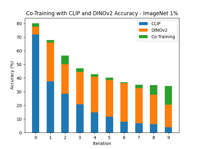
Figure 7: Top-1 accuracy of co-training iterations on the CLIP and DINOv2 views for the ImageNet 1% dataset.

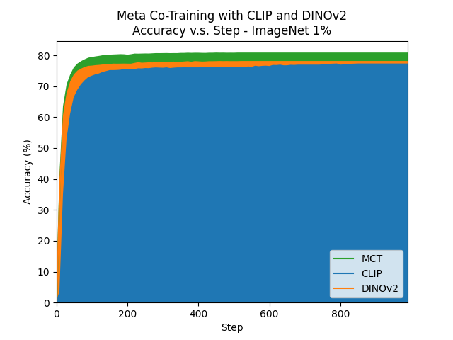
Figure 8: Meta co-training using the CLIP and DINOv2 views as a function of the training step. Models are trained on 1% of the ImageNet labels.

Similar to the case of ImageNet 10% we see that the co-training performance decreases after the supervised warmup. Unlike co-training, meta co-training performance increases after the supervised warmup.

Figures 9 and 10 are comparable to Figures 5 and 6 in the main text, but for the ImageNet-1% dataset.

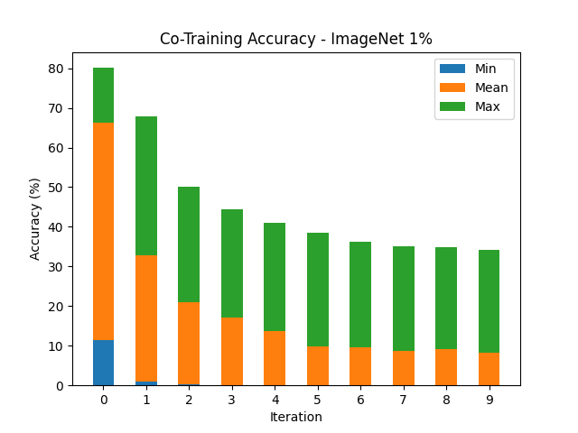
Figure 9: Top-1 accuracy of co-training iterations for the ImageNet 1% dataset. The average over all 10 pairs, the best pair, and the worst pair at each iteration are shown.

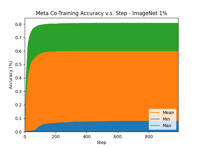
Figure 10: Aggregate statistics of meta co-training across all views. Models are trained on 1% of the ImageNet labels. The maximum performance of any pair, the minimum performance of any pair, and the average of all 10 pairs is shown.

The min, max, and mean performance of any of the ten pairs is shown. Note that these are not three runs, but aggregate statistics over all runs, so the minimum and maximum points on the graph for one step may not correspond to the same pair as another step.

Appendix B Further Experimental Analysis on Datasets Beyond ImageNet

Figures 11, 12, 13, 14, 15, 16, and 17 include the top-1 accuracy of co-training using the best (CLIP and DINO) views found for the ImageNet task. In all cases except Figure 11, co-training reaches its maximum performance in the first (warmup) iteration where training is strictly supervised with no pseudo labels. Note that there is no 1% run for Flowers102 because there are only 10 examples for each class in the training set (see the discussion in Section C).

B.1 Co-Training and Meta Co-Training on Food101

In Figures 11 and  12 we show the top-1 accuracy of the iterations of co-training on the Food101 classification task. Co-training performs as expected with the pseudo labels allowing the other model to improve in the 10% case, but in the 1% case it appears that one or more of the views was insufficient and the performance decreases rapidly after the first iteration. Co-training achieves top-1 accuracy of 94.7% (resp., 83.9%) when 10% (resp., 1%) of the available labels for training are used from the Food101 dataset.

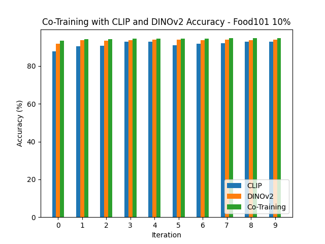
Figure 11: The top-1 accuracy of the co-training predictions for each iteration of co-training. 10% of available Food101 labels are used for training. The method exhibits performance improvement over multiple iterations of pseudo-labeling and retraining.

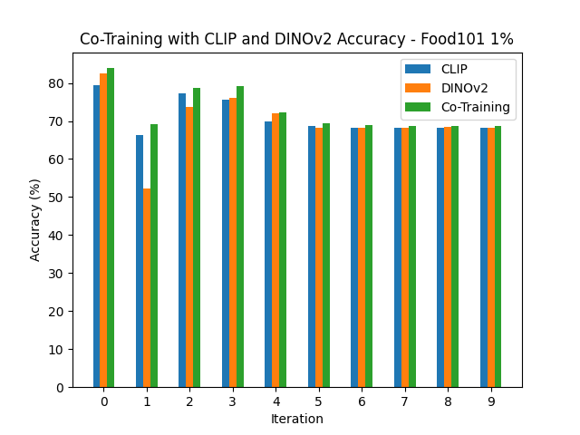
Figure 12: The top-1 accuracy of the co-training predictions for each iteration of co-training. 1% of available Food101 labels are used for training.

Similarly, meta co-training achieves top-1 accuracy of 94.8% (resp., 91.7%) when 10% (resp., 1%) of the available training examples of the Food101 dataset are used.

These results are compared against each other as well as against REACT and Semi-ViT in Tables 7 and 8 respectively.

B.2 Co-Training and Meta Co-Training on iNaturalist

In Figures 13 and 14 we show the top-1 accuracy of the iterations of co-training on the iNaturalist dataset.

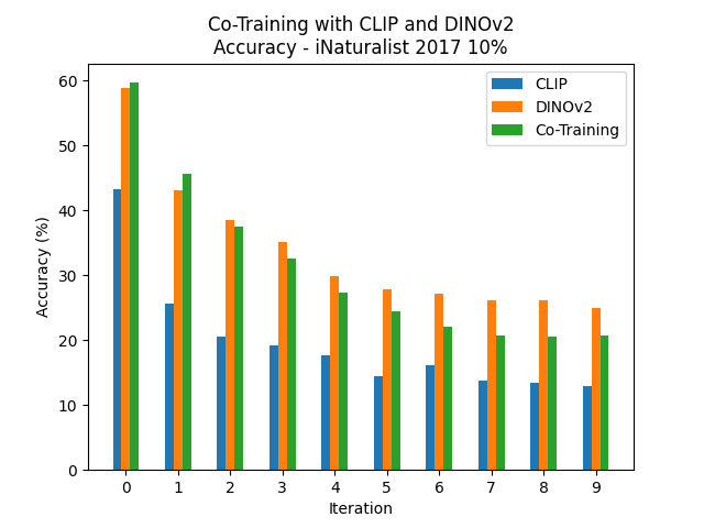
Figure 13: The top-1 accuracy of the co-training predictions for each iteration of co-training. Only the 1010 most frequent classes are included. 10% of available iNaturalist labels from those classes are used for training.

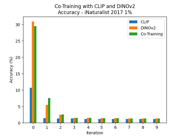
Figure 14: The top-1 accuracy of the co-training predictions for each iteration of co-training. Only the 1010 most frequent classes are included. 1% of available iNaturalist labels from those classes are used for training.

In both splits we see a steady decline in top-1 accuracy after the first iteration. Co-training achieves top-1 accuracy of 59.7% (resp., 29.5%) when only 10% (resp., 1%) of the training examples of the iNaturalist dataset are used.

Along these lines meta co-training achieves 76.0% (resp., 58.1%) when only 10% (resp., 1%) of the training examples of the iNaturalist dataset are used.

These results are compared against each other as well as against REACT and Semi-ViT in Tables 7 and 8 respectively.

B.3 Co-Training and Meta Co-Training on CTFGVCAircraft

In Figures 15 and 16 we show the top-1 accuracy of the iterations of co-training on the CTFGVCAircraft dataset.

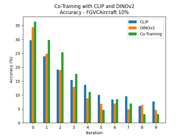
Figure 15: The top-1 accuracy of the co-training predictions for each iteration of co-training. 10% of available FGVCAircraft labels are used for training.

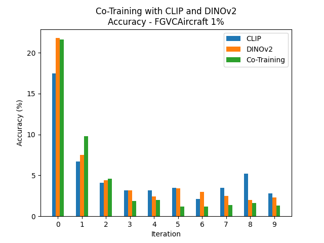
Figure 16: The top-1 accuracy of the co-training predictions for each iteration of co-training. 1% of available FGVCAircraft labels are used for training.

In both cases both views have low accuracy, so it is unsurprising that in subsequent iterations the accuracy decreases rapidly. In particular, co-training achieves top-1 accuracy of 36.4% (resp., 21.6%) when only 10% (resp., 1%) of the training examples of the CTFGVCAircraft dataset are used.

Along these lines meta co-training achieves 40.1% (resp., 21.5%) when only 10% (resp., 1%) of the training examples of the CTFGVCAircraft dataset are used.

The results corresponding to the 10% case of co-training and meta co-training are compared against REACT in Table 7, since the authors of [52] report results on zero-shot and 10% cases only. However, for completeness, we have decided to include Figure 16 which corresponds to the experiments that we did using only 1% of the labeled training data available for the CTFGVCAircraft dataset.

B.4 Co-Training and Meta Co-Training on Flowers102

As explained earlier, the Flowers102 dataset has only 10 training examples for each class and hence 10% corresponds to 1-shot learning. In this context, in Figure 17 we give the performance of the iterations of co-training on the Flowers102 dataset.

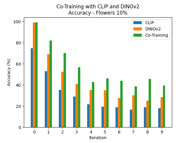
Figure 17: The top-1 accuracy of the co-training predictions for each iteration of co-training. 10% of available Flowers102 labels are used for training.

Even though the DINO view performs very well in the first iteration, there is a large gap between the performance of the CLIP view and the DINO view which leads to decreased performance in subsequent iterations. Co-training achieves top-1 accuracy of 99.2% when only 10% of the training examples of the Flowers102 dataset are used for training (i.e., a single labeled image per class).

In the same context of 1-shot learning, meta co-training achieves top-1 accuracy of 99.6%.

Both of the above results are compared against each other and against REACT in Table 7.

Appendix C Further Information on the Datasets and the Splits

Table 9 includes a description of the different sizes of the datasets used for training and testing, as well as the number of cases for each dataset.

Dataset	#train	#test	#classes
FGVCAircraft	3333	3333	100
Flowers102	1020	6149	102
Food101	75,750	25,250	101
iNaturalist	175,489	29,083	1010
ImageNet	1,281,167	50,000	1000

Table 9: Sizes of datasets used. Subsets drawn for training are always drawn in a stratified way to maintain the class distribution of the original data. For ImageNet we use the split published with the SimCLRv2 [24] repository.

Note that in the 10% experiments on the Flowers102 dataset each class has only 1 label. All datasets are approximately class-balanced with the exception of the iNaturalist dataset. In all cases we maintain the original class distribution when sampling subsets. All subsets are created with seeded randomness of a common seed (13) which ensures a fair comparison between methods.

Appendix D Hyperparameter Configuration

The relevant hyperparameters for training are included in Table 10 for co-training and meta co-training (MCT).

config	MCT	Co-Training
optimizer	Adam	Adam
optimizer momentum	$\beta_{1},\beta_{2}=0.9,0.999$	$\beta_{1},\beta_{2}=0.9,0.999$
base learning rate	1e-4	1e-4
batch size	4096	4096
learning rate schedule	Reduce On Plateau	Reduce On Plateau
schedule patience	10 steps	10 steps
decay factor	0.5	0.5
training steps	1000	200 (per iteration)
warmup steps	200	n/a

Table 10: Hyperparmeter configuration for meta co-training and co-training. Other models used (MLP, linear) are trained for the same number of steps as meta co-training, with the same optimization parameters.

References

- [1] Dana Angluin and Philip D. Laird. Learning From Noisy Examples. Mach. Learn., 2(4):343–370, 1987.
- [2] Eric Arazo, Diego Ortego, Paul Albert, Noel E. O’Connor, and Kevin McGuinness. Pseudo-Labeling and Confirmation Bias in Deep Semi-Supervised Learning. In 2020 International Joint Conference on Neural Networks, IJCNN 2020, Glasgow, United Kingdom, July 19-24, 2020, pages 1–8. IEEE, 2020.
- [3] Yuki Markus Asano, Christian Rupprecht, and Andrea Vedaldi. Self-labelling via simultaneous clustering and representation learning. In 8th International Conference on Learning Representations, ICLR 2020, Addis Ababa, Ethiopia, April 26-30, 2020. OpenReview.net, 2020.
- [4] Maria-Florina Balcan and Avrim Blum. An Augmented PAC Model for Semi-Supervised Learning. In Olivier Chapelle, Bernhard Schölkopf, and Alexander Zien, editors, Semi-Supervised Learning, pages 396–419. The MIT Press, 2006.
- [5] Maria-Florina Balcan, Avrim Blum, and Ke Yang. Co-Training and Expansion: Towards Bridging Theory and Practice. In Advances in Neural Information Processing Systems 17 [Neural Information Processing Systems, NeurIPS 2004, December 13-18, 2004, Vancouver, British Columbia, Canada], pages 89–96, 2004.
- [6] Maria-Florina Balcan and Dravyansh Sharma. Data driven semi-supervised learning. In Marc’Aurelio Ranzato, Alina Beygelzimer, Yann N. Dauphin, Percy Liang, and Jennifer Wortman Vaughan, editors, Advances in Neural Information Processing Systems 34: Annual Conference on Neural Information Processing Systems 2021, NeurIPS 2021, December 6-14, 2021, virtual, pages 14782–14794, 2021.
- [7] Shumeet Baluja. Probabilistic Modeling for Face Orientation Discrimination: Learning from Labeled and Unlabeled Data. In Michael J. Kearns, Sara A. Solla, and David A. Cohn, editors, Advances in Neural Information Processing Systems 11, [NeurIPS Conference, Denver, Colorado, USA, November 30 - December 5, 1998], pages 854–860. The MIT Press, 1998.
- [8] Adrien Bardes, Jean Ponce, and Yann LeCun. VICReg: Variance-Invariance-Covariance Regularization for Self-Supervised Learning. In The Tenth International Conference on Learning Representations, ICLR 2022, Virtual Event, April 25-29, 2022. OpenReview.net, 2022.
- [9] Sugato Basu, Ian Davidson, and Kiri Wagstaff. Constrained clustering: Advances in algorithms, theory, and applications. CRC Press, 2008.
- [10] Mikhail Belkin, Partha Niyogi, and Vikas Sindhwani. Manifold Regularization: A Geometric Framework for Learning from Labeled and Unlabeled Examples. Journal of Machine Learning Research, 7:2399–2434, 2006.
- [11] Avrim Blum, John D. Lafferty, Mugizi Robert Rwebangira, and Rajashekar Reddy. Semi-supervised learning using randomized mincuts. In Carla E. Brodley, editor, Machine Learning, Proceedings of the Twenty-first International Conference (ICML 2004), Banff, Alberta, Canada, July 4-8, 2004, volume 69 of ACM International Conference Proceeding Series. ACM, 2004.
- [12] Avrim Blum and Tom M. Mitchell. Combining Labeled and Unlabeled Data with Co-Training. In Peter L. Bartlett and Yishay Mansour, editors, Proceedings of the Eleventh Annual Conference on Computational Learning Theory, COLT 1998, Madison, Wisconsin, USA, July 24-26, 1998, pages 92–100. ACM, 1998.
- [13] Avrim Blum and Ronald L. Rivest. Training a 3-Node Neural Network is NP-Complete. In Stephen Jose Hanson, Werner Remmele, and Ronald L. Rivest, editors, Machine Learning: From Theory to Applications - Cooperative Research at Siemens and MIT, volume 661 of Lecture Notes in Computer Science, pages 9–28. Springer, 1993.
- [14] Lukas Bossard, Matthieu Guillaumin, and Luc Van Gool. Food-101 - Mining Discriminative Components with Random Forests. In David J. Fleet, Tomás Pajdla, Bernt Schiele, and Tinne Tuytelaars, editors, Computer Vision - ECCV 2014 - 13th European Conference, Zurich, Switzerland, September 6-12, 2014, Proceedings, Part VI, volume 8694 of Lecture Notes in Computer Science, pages 446–461. Springer, 2014.
- [15] Ulf Brefeld, Christoph Büscher, and Tobias Scheffer. Multi-view Discriminative Sequential Learning. In João Gama, Rui Camacho, Pavel Brazdil, Alípio Jorge, and Luís Torgo, editors, Machine Learning: ECML 2005, 16th European Conference on Machine Learning, Porto, Portugal, October 3-7, 2005, Proceedings, volume 3720 of Lecture Notes in Computer Science, pages 60–71. Springer, 2005.
- [16] Ulf Brefeld and Tobias Scheffer. Co-EM support vector learning. In Carla E. Brodley, editor, Machine Learning, Proceedings of the Twenty-first International Conference (ICML 2004), Banff, Alberta, Canada, July 4-8, 2004, volume 69 of ACM International Conference Proceeding Series. ACM, 2004.
- [17] Zhaowei Cai, Avinash Ravichandran, Paolo Favaro, Manchen Wang, Davide Modolo, Rahul Bhotika, Zhuowen Tu, and Stefano Soatto. Semi-supervised Vision Transformers at Scale. In NeurIPS, 2022.
- [18] Mathilde Caron, Piotr Bojanowski, Armand Joulin, and Matthijs Douze. Deep Clustering for Unsupervised Learning of Visual Features. In Vittorio Ferrari, Martial Hebert, Cristian Sminchisescu, and Yair Weiss, editors, Computer Vision - ECCV 2018 - 15th European Conference, Munich, Germany, September 8-14, 2018, Proceedings, Part XIV, volume 11218 of Lecture Notes in Computer Science, pages 139–156. Springer, 2018.
- [19] Mathilde Caron, Ishan Misra, Julien Mairal, Priya Goyal, Piotr Bojanowski, and Armand Joulin. Unsupervised Learning of Visual Features by Contrasting Cluster Assignments. In Hugo Larochelle, Marc’Aurelio Ranzato, Raia Hadsell, Maria-Florina Balcan, and Hsuan-Tien Lin, editors, Advances in Neural Information Processing Systems 33: Annual Conference on Neural Information Processing Systems 2020, NeurIPS 2020, December 6-12, 2020, virtual, 2020.
- [20] Mathilde Caron, Hugo Touvron, Ishan Misra, Hervé Jégou, Julien Mairal, Piotr Bojanowski, and Armand Joulin. Emerging Properties in Self-Supervised Vision Transformers. In 2021 IEEE/CVF International Conference on Computer Vision, ICCV 2021, Montreal, QC, Canada, October 10-17, 2021, pages 9630–9640. IEEE, 2021.
- [21] Olivier Chapelle, Bernhard Schölkopf, and Alexander Zien, editors. Semi-Supervised Learning. The MIT Press, 2006.
- [22] Minmin Chen, Kilian Q. Weinberger, and Yixin Chen. Automatic Feature Decomposition for Single View Co-training. In Lise Getoor and Tobias Scheffer, editors, Proceedings of the 28th International Conference on Machine Learning, ICML 2011, Bellevue, Washington, USA, June 28 - July 2, 2011, pages 953–960. Omnipress, 2011.
- [23] Ting Chen, Simon Kornblith, Mohammad Norouzi, and Geoffrey E. Hinton. A Simple Framework for Contrastive Learning of Visual Representations. In Proceedings of the 37th International Conference on Machine Learning, ICML 2020, 13-18 July 2020, Virtual Event, volume 119 of Proceedings of Machine Learning Research, pages 1597–1607. PMLR, 2020.
- [24] Ting Chen, Simon Kornblith, Kevin Swersky, Mohammad Norouzi, and Geoffrey E. Hinton. Big Self-Supervised Models are Strong Semi-Supervised Learners. In Hugo Larochelle, Marc’Aurelio Ranzato, Raia Hadsell, Maria-Florina Balcan, and Hsuan-Tien Lin, editors, Advances in Neural Information Processing Systems 33: Annual Conference on Neural Information Processing Systems 2020, NeurIPS 2020, December 6-12, 2020, virtual, 2020.
- [25] Malte Darnstädt, Hans Ulrich Simon, and Balázs Szörényi. Unlabeled Data Does Provably Help. In Natacha Portier and Thomas Wilke, editors, 30th International Symposium on Theoretical Aspects of Computer Science, STACS 2013, February 27 - March 2, 2013, Kiel, Germany, volume 20 of LIPIcs, pages 185–196. Schloss Dagstuhl - Leibniz-Zentrum für Informatik, 2013.
- [26] Malte Darnstädt, Hans Ulrich Simon, and Balázs Szörényi. Supervised learning and Co-training. Theor. Comput. Sci., 519:68–87, 2014.
- [27] Sanjoy Dasgupta, Michael L. Littman, and David A. McAllester. PAC Generalization Bounds for Co-training. In Thomas G. Dietterich, Suzanna Becker, and Zoubin Ghahramani, editors, Advances in Neural Information Processing Systems 14 [Neural Information Processing Systems: Natural and Synthetic, NeurIPS 2001, December 3-8, 2001, Vancouver, British Columbia, Canada], pages 375–382. MIT Press, 2001.
- [28] Ian Davidson and S. S. Ravi. Agglomerative Hierarchical Clustering with Constraints: Theoretical and Empirical Results. In Alípio Jorge, Luís Torgo, Pavel Brazdil, Rui Camacho, and João Gama, editors, Knowledge Discovery in Databases: PKDD 2005, 9th European Conference on Principles and Practice of Knowledge Discovery in Databases, Porto, Portugal, October 3-7, 2005, Proceedings, volume 3721 of Lecture Notes in Computer Science, pages 59–70. Springer, 2005.
- [29] Neil E Day. Estimating the components of a mixture of normal distributions. Biometrika, 56(3):463–474, 1969.
- [30] Arthur P Dempster, Nan M Laird, and Donald B Rubin. Maximum likelihood from incomplete data via the EM algorithm. Journal of the Royal Statistical Society: Series B (Methodological), 39(1):1–22, 1977.
- [31] Jia Deng, Wei Dong, Richard Socher, Li-Jia Li, Kai Li, and Li Fei-Fei. ImageNet: A large-scale hierarchical image database. In 2009 IEEE Computer Society Conference on Computer Vision and Pattern Recognition (CVPR 2009), 20-25 June 2009, Miami, Florida, USA, pages 248–255. IEEE Computer Society, 2009.
- [32] Jacob Devlin, Ming-Wei Chang, Kenton Lee, and Kristina Toutanova. BERT: Pre-training of Deep Bidirectional Transformers for Language Understanding. In Jill Burstein, Christy Doran, and Thamar Solorio, editors, Proceedings of the 2019 Conference of the North American Chapter of the Association for Computational Linguistics: Human Language Technologies, NAACL-HLT 2019, Minneapolis, MN, USA, June 2-7, 2019, Volume 1 (Long and Short Papers), pages 4171–4186. Association for Computational Linguistics, 2019.
- [33] Wei Di and Melba M. Crawford. View Generation for Multiview Maximum Disagreement Based Active Learning for Hyperspectral Image Classification. IEEE Trans. Geosci. Remote. Sens., 50(5-2):1942–1954, 2012.
- [34] Jun Du, Charles X. Ling, and Zhi-Hua Zhou. When Does Cotraining Work in Real Data? IEEE Transactions on Knowledge and Data Engineering, 23(5):788–799, 2011.
- [35] Chelsea Finn, Pieter Abbeel, and Sergey Levine. Model-Agnostic Meta-Learning for Fast Adaptation of Deep Networks. In Doina Precup and Yee Whye Teh, editors, Proceedings of the 34th International Conference on Machine Learning, ICML 2017, Sydney, NSW, Australia, 6-11 August 2017, volume 70 of Proceedings of Machine Learning Research, pages 1126–1135. PMLR, 2017.
- [36] S Fralick. Learning to recognize patterns without a teacher. IEEE Transactions on Information Theory, 13(1):57–64, 1967.
- [37] Alexander Golovnev, Dávid Pál, and Balázs Szörényi. The information-theoretic value of unlabeled data in semi-supervised learning. In Kamalika Chaudhuri and Ruslan Salakhutdinov, editors, Proceedings of the 36th International Conference on Machine Learning, ICML 2019, 9-15 June 2019, Long Beach, California, USA, volume 97 of Proceedings of Machine Learning Research, pages 2328–2336. PMLR, 2019.
- [38] Jean-Bastien Grill, Florian Strub, Florent Altché, Corentin Tallec, Pierre H. Richemond, Elena Buchatskaya, Carl Doersch, Bernardo Ávila Pires, Zhaohan Guo, Mohammad Gheshlaghi Azar, Bilal Piot, Koray Kavukcuoglu, Rémi Munos, and Michal Valko. Bootstrap Your Own Latent - A New Approach to Self-Supervised Learning. In Hugo Larochelle, Marc’Aurelio Ranzato, Raia Hadsell, Maria-Florina Balcan, and Hsuan-Tien Lin, editors, Advances in Neural Information Processing Systems 33: Annual Conference on Neural Information Processing Systems 2020, NeurIPS 2020, December 6-12, 2020, virtual, 2020.
- [39] Xiaowei Gu. A self-training hierarchical prototype-based approach for semi-supervised classification. Inf. Sci., 535:204–224, 2020.
- [40] Zeyad Hailat and Xue-wen Chen. Teacher/Student Deep Semi-Supervised Learning for Training with Noisy Labels. In M. Arif Wani, Mehmed M. Kantardzic, Moamar Sayed Mouchaweh, João Gama, and Edwin Lughofer, editors, 17th IEEE International Conference on Machine Learning and Applications, ICMLA 2018, Orlando, FL, USA, December 17-20, 2018, pages 907–912. IEEE, 2018.
- [41] Herman Otto Hartley and Jon NK Rao. Classification and estimation in analysis of variance problems. Revue de l’Institut International de Statistique, pages 141–147, 1968.
- [42] Kaiming He, Xinlei Chen, Saining Xie, Yanghao Li, Piotr Dollár, and Ross B. Girshick. Masked Autoencoders Are Scalable Vision Learners. In IEEE/CVF Conference on Computer Vision and Pattern Recognition, CVPR 2022, New Orleans, LA, USA, June 18-24, 2022, pages 15979–15988. IEEE, 2022.
- [43] Kaiming He, Haoqi Fan, Yuxin Wu, Saining Xie, and Ross B. Girshick. Momentum Contrast for Unsupervised Visual Representation Learning. In 2020 IEEE/CVF Conference on Computer Vision and Pattern Recognition, CVPR 2020, Seattle, WA, USA, June 13-19, 2020, pages 9726–9735. Computer Vision Foundation / IEEE, 2020.
- [44] Grant Van Horn, Oisin Mac Aodha, Yang Song, Yin Cui, Chen Sun, Alexander Shepard, Hartwig Adam, Pietro Perona, and Serge J. Belongie. The INaturalist Species Classification and Detection Dataset. In 2018 IEEE Conference on Computer Vision and Pattern Recognition, CVPR 2018, Salt Lake City, UT, USA, June 18-22, 2018, pages 8769–8778. Computer Vision Foundation / IEEE Computer Society, 2018.
- [45] Grant Van Horn, Elijah Cole, Sara Beery, Kimberly Wilber, Serge J. Belongie, and Oisin Mac Aodha. Benchmarking Representation Learning for Natural World Image Collections. In IEEE Conference on Computer Vision and Pattern Recognition, CVPR 2021, virtual, June 19-25, 2021, pages 12884–12893. Computer Vision Foundation / IEEE, 2021.
- [46] Soroush Abbasi Koohpayegani, Ajinkya Tejankar, and Hamed Pirsiavash. Mean Shift for Self-Supervised Learning. In 2021 IEEE/CVF International Conference on Computer Vision, ICCV 2021, Montreal, QC, Canada, October 10-17, 2021, pages 10306–10315. IEEE, 2021.
- [47] Samuli Laine and Timo Aila. Temporal Ensembling for Semi-Supervised Learning. In 5th International Conference on Learning Representations, ICLR 2017, Toulon, France, April 24-26, 2017, Conference Track Proceedings. OpenReview.net, 2017.
- [48] Dong-Hyun Lee. Pseudo-Label : The Simple and Efficient Semi-Supervised Learning Method for Deep Neural Networks. Workshop on Challenges in Representation Learning, ICML, 3(2):896, 2013.
- [49] Chunyuan Li, Jianwei Yang, Pengchuan Zhang, Mei Gao, Bin Xiao, Xiyang Dai, Lu Yuan, and Jianfeng Gao. Efficient Self-supervised Vision Transformers for Representation Learning. In The Tenth International Conference on Learning Representations, ICLR 2022, Virtual Event, April 25-29, 2022. OpenReview.net, 2022.
- [50] Xinzhe Li, Qianru Sun, Yaoyao Liu, Qin Zhou, Shibao Zheng, Tat-Seng Chua, and Bernt Schiele. Learning to Self-Train for Semi-Supervised Few-Shot Classification. In Hanna M. Wallach, Hugo Larochelle, Alina Beygelzimer, Florence d’Alché-Buc, Emily B. Fox, and Roman Garnett, editors, Advances in Neural Information Processing Systems 32: Annual Conference on Neural Information Processing Systems 2019, NeurIPS 2019, December 8-14, 2019, Vancouver, BC, Canada, pages 10276–10286, 2019.
- [51] Hanxiao Liu, Karen Simonyan, and Yiming Yang. DARTS: Differentiable Architecture Search. In 7th International Conference on Learning Representations, ICLR 2019, New Orleans, LA, USA, May 6-9, 2019. OpenReview.net, 2019.
- [52] Haotian Liu, Kilho Son, Jianwei Yang, Ce Liu, Jianfeng Gao, Yong Jae Lee, and Chunyuan Li. Learning Customized Visual Models with Retrieval-Augmented Knowledge. In IEEE/CVF Conference on Computer Vision and Pattern Recognition, CVPR 2023, Vancouver, BC, Canada, June 17-24, 2023, pages 15148–15158. IEEE, 2023.
- [53] Yucen Luo, Jun Zhu, Mengxi Li, Yong Ren, and Bo Zhang. Smooth Neighbors on Teacher Graphs for Semi-Supervised Learning. In 2018 IEEE Conference on Computer Vision and Pattern Recognition, CVPR 2018, Salt Lake City, UT, USA, June 18-22, 2018, pages 8896–8905. Computer Vision Foundation / IEEE Computer Society, 2018.
- [54] S. Maji, J. Kannala, E. Rahtu, M. Blaschko, and A. Vedaldi. Fine-Grained Visual Classification of Aircraft. Technical report, Visual Geometry Group, University of Oxford, 2013.
- [55] Pavan Kumar Mallapragada, Rong Jin, Anil K. Jain, and Yi Liu. SemiBoost: Boosting for Semi-Supervised Learning. IEEE Trans. Pattern Anal. Mach. Intell., 31(11):2000–2014, 2009.
- [56] Kamal Nigam and Rayid Ghani. Analyzing the Effectiveness and Applicability of Co-training. In Proceedings of the 2000 ACM CIKM International Conference on Information and Knowledge Management, McLean, VA, USA, November 6-11, 2000, pages 86–93. ACM, 2000.
- [57] Maria-Elena Nilsback and Andrew Zisserman. Automated Flower Classification over a Large Number of Classes. In Sixth Indian Conference on Computer Vision, Graphics & Image Processing, ICVGIP 2008, Bhubaneswar, India, 16-19 December 2008, pages 722–729. IEEE Computer Society, 2008.
- [58] Maxime Oquab, Timothée Darcet, Théo Moutakanni, Huy Vo, Marc Szafraniec, Vasil Khalidov, Pierre Fernandez, Daniel Haziza, Francisco Massa, Alaaeldin El-Nouby, Mahmoud Assran, Nicolas Ballas, Wojciech Galuba, Russell Howes, Po-Yao Huang, Shang-Wen Li, Ishan Misra, Michael G. Rabbat, Vasu Sharma, Gabriel Synnaeve, Hu Xu, Hervé Jégou, Julien Mairal, Patrick Labatut, Armand Joulin, and Piotr Bojanowski. DINOv2: Learning Robust Visual Features without Supervision. CoRR, abs/2304.07193, 2023.
- [59] Hieu Pham, Zihang Dai, Qizhe Xie, and Quoc V. Le. Meta Pseudo Labels. In IEEE Conference on Computer Vision and Pattern Recognition, CVPR 2021, virtual, June 19-25, 2021, pages 11557–11568. Computer Vision Foundation / IEEE, 2021.
- [60] Siyuan Qiao, Wei Shen, Zhishuai Zhang, Bo Wang, and Alan L. Yuille. Deep Co-Training for Semi-Supervised Image Recognition. In Vittorio Ferrari, Martial Hebert, Cristian Sminchisescu, and Yair Weiss, editors, Computer Vision - ECCV 2018 - 15th European Conference, Munich, Germany, September 8-14, 2018, Proceedings, Part XV, volume 11219 of Lecture Notes in Computer Science, pages 142–159. Springer, 2018.
- [61] Alec Radford, Jong Wook Kim, Chris Hallacy, Aditya Ramesh, Gabriel Goh, Sandhini Agarwal, Girish Sastry, Amanda Askell, Pamela Mishkin, Jack Clark, Gretchen Krueger, and Ilya Sutskever. Learning Transferable Visual Models From Natural Language Supervision. In Marina Meila and Tong Zhang, editors, Proceedings of the 38th International Conference on Machine Learning, ICML 2021, 18-24 July 2021, Virtual Event, volume 139 of Proceedings of Machine Learning Research, pages 8748–8763. PMLR, 2021.
- [62] Christoph Schuhmann, Romain Beaumont, Richard Vencu, Cade Gordon, Ross Wightman, Mehdi Cherti, Theo Coombes, Aarush Katta, Clayton Mullis, Mitchell Wortsman, Patrick Schramowski, Srivatsa Kundurthy, Katherine Crowson, Ludwig Schmidt, Robert Kaczmarczyk, and Jenia Jitsev. LAION-5B: An open large-scale dataset for training next generation image-text models. In NeurIPS, 2022.
- [63] Christoph Schuhmann, Richard Vencu, Romain Beaumont, Robert Kaczmarczyk, Clayton Mullis, Aarush Katta, Theo Coombes, Jenia Jitsev, and Aran Komatsuzaki. LAION-400M: Open Dataset of CLIP-Filtered 400 Million Image-Text Pairs. In Data Centric AI NeurIPS Workshop, 2021.
- [64] Henry Scudder. Probability of error of some adaptive pattern-recognition machines. IEEE Transactions on Information Theory, 11(3):363–371, 1965.
- [65] Shiliang Sun, Feng Jin, and Wenting Tu. View Construction for Multi-view Semi-supervised Learning. In Derong Liu, Huaguang Zhang, Marios M. Polycarpou, Cesare Alippi, and Haibo He, editors, Advances in Neural Networks - ISNN 2011 - 8th International Symposium on Neural Networks, ISNN 2011, Guilin, China, May 29-June 1, 2011, Proceedings, Part I, volume 6675 of Lecture Notes in Computer Science, pages 595–601. Springer, 2011.
- [66] Ajinkya Tejankar, Soroush Abbasi Koohpayegani, Vipin Pillai, Paolo Favaro, and Hamed Pirsiavash. ISD: Self-Supervised Learning by Iterative Similarity Distillation. In 2021 IEEE/CVF International Conference on Computer Vision, ICCV 2021, Montreal, QC, Canada, October 10-17, 2021, pages 9589–9598. IEEE, 2021.
- [67] Jesper E. van Engelen and Holger H. Hoos. A survey on semi-supervised learning. Machine Learning, 109(2):373–440, 2020.
- [68] Kiri Wagstaff, Sugato Basu, and Ian Davidson. When Is Constrained Clustering Beneficial, and Why? In Proceedings, The Twenty-First National Conference on Artificial Intelligence and the Eighteenth Innovative Applications of Artificial Intelligence Conference, July 16-20, 2006, Boston, Massachusetts, USA. AAAI Press, 2006.
- [69] Kiri Wagstaff, Claire Cardie, Seth Rogers, and Stefan Schrödl. Constrained K-means Clustering with Background Knowledge. In Carla E. Brodley and Andrea Pohoreckyj Danyluk, editors, Proceedings of the Eighteenth International Conference on Machine Learning (ICML 2001), Williams College, Williamstown, MA, USA, June 28 - July 1, 2001, pages 577–584. Morgan Kaufmann, 2001.
- [70] Jun Wang, Tony Jebara, and Shih-Fu Chang. Semi-Supervised Learning Using Greedy Max-Cut. J. Mach. Learn. Res., 14(1):771–800, 2013.
- [71] Jiao Wang, Siwei Luo, and Xianhua Zeng. A random subspace method for co-training. In Proceedings of the International Joint Conference on Neural Networks, IJCNN 2008, part of the IEEE World Congress on Computational Intelligence, WCCI 2008, Hong Kong, China, June 1-6, 2008, pages 195–200. IEEE, 2008.
- [72] Chen Wei, Kihyuk Sohn, Clayton Mellina, Alan L. Yuille, and Fan Yang. CReST: A Class-Rebalancing Self-Training Framework for Imbalanced Semi-Supervised Learning. In IEEE Conference on Computer Vision and Pattern Recognition, CVPR 2021, virtual, June 19-25, 2021, pages 10857–10866. Computer Vision Foundation / IEEE, 2021.
- [73] Jason Weston, Frédéric Ratle, Hossein Mobahi, and Ronan Collobert. Deep Learning via Semi-supervised Embedding. In Grégoire Montavon, Genevieve B. Orr, and Klaus-Robert Müller, editors, Neural Networks: Tricks of the Trade - Second Edition, volume 7700 of Lecture Notes in Computer Science, pages 639–655. Springer, 2012.
- [74] Hao Wu and Saurabh Prasad. Semi-Supervised Deep Learning Using Pseudo Labels for Hyperspectral Image Classification. IEEE Trans. Image Process., 27(3):1259–1270, 2018.
- [75] Qizhe Xie, Zihang Dai, Eduard H. Hovy, Thang Luong, and Quoc Le. Unsupervised Data Augmentation for Consistency Training. In Hugo Larochelle, Marc’Aurelio Ranzato, Raia Hadsell, Maria-Florina Balcan, and Hsuan-Tien Lin, editors, Advances in Neural Information Processing Systems 33: Annual Conference on Neural Information Processing Systems 2020, NeurIPS 2020, December 6-12, 2020, virtual, 2020.
- [76] Qizhe Xie, Minh-Thang Luong, Eduard H. Hovy, and Quoc V. Le. Self-Training With Noisy Student Improves ImageNet Classification. In 2020 IEEE/CVF Conference on Computer Vision and Pattern Recognition, CVPR 2020, Seattle, WA, USA, June 13-19, 2020, pages 10684–10695. Computer Vision Foundation / IEEE, 2020.
- [77] Zhi-Hua Zhou and Ming Li. Tri-Training: Exploiting Unlabeled Data Using Three Classifiers. IEEE Trans. Knowl. Data Eng., 17(11):1529–1541, 2005.
- [78] Xiaojin Zhu and Andrew B. Goldberg. Introduction to Semi-Supervised Learning. Synthesis Lectures on Artificial Intelligence and Machine Learning. Morgan & Claypool Publishers, 2009.
- [79] Barret Zoph, Golnaz Ghiasi, Tsung-Yi Lin, Yin Cui, Hanxiao Liu, Ekin Dogus Cubuk, and Quoc Le. Rethinking Pre-training and Self-training. In Hugo Larochelle, Marc’Aurelio Ranzato, Raia Hadsell, Maria-Florina Balcan, and Hsuan-Tien Lin, editors, Advances in Neural Information Processing Systems 33: Annual Conference on Neural Information Processing Systems 2020, NeurIPS 2020, December 6-12, 2020, virtual, 2020.