Page curve entanglement dynamics in an analytically solvable model

Abstract

The entanglement entropy of black holes is expected to follow the Page curve. After an initial linear increase with time the entanglement entropy should reach a maximum at the Page time and then decrease. This bending down of the Page curve and the apparent contradiction with Hawking’s semiclassical calculation from 1975 is at the center of the black hole information paradox. Motivated by this – from the point of view of non-equilibrium quantum many-body systems – unusual behavior of the entanglement entropy, this paper introduces an exactly solvable model of free fermions that explicitly shows such a Page curve: The entanglement entropy vanishes asymptotically for late times instead of saturating at a volume law. Physical observables like the particle current do not show any unusual behavior at the Page time and one can explicitly see how the semiclassical connection between particle current and entanglement generation breaks down.

Introduction. The study of entanglement properties has become an important tool across many fields of physics from condensed matter physics to quantum information theory and black hole physics, bringing about remarkable and fruitful connections between these different fields. One example is the universal area law for ground states of local Hamiltonians Eisert et al. (2010), which is e.g. central for computational matrix product methods Schollwöck (2011), but also for holography Ryu and Takayanagi (2006). Likewise in non-equilibrium much can be learned from the entanglement dynamics: Generically, the entanglement entropy of ergodic systems grows linearly in time until it saturates at a value given by the volume law for excited states. For systems with well-defined quasiparticles the underlying mechanism for this behavior is the local generation of entangled pairs of quasiparticles, whose propagation leads to entanglement of separate spatial regions Calabrese and Cardy (2005). While the general validity of this behavior has been confirmed by many analytical and numerical studies (see e.g. Ref. Ho and Abanin (2017)), even for systems with diffusive energy transport Kim and Huse (2013), a long standing debate in black hole physics centers around the very different entanglement dynamics described by the Page curve resulting from the decay of a black hole.

The first part of the Page curve, that is a linearly increasing entanglement entropy up to the Page time, is perfectly consistent with the above picture: Hawking’s semiclassical calculation in 1975 Hawking (1975) established the production of particle pairs at the event horizon, with one particle escaping to infinity and generating black body radiation with the Hawking temperature. The other particle from the pair falls into the singularity and reduces the mass of the black hole. The entanglement of these particle pairs leads to linearly growing entanglement between the black hole and the enviroment (or equivalently the Hawking radiation). However, as pointed out by Page Page (1993, 2013), once the black hole has decayed to about half its original mass, there are not enough degrees of freedom left in the Hilbert space of the black hole to let the entanglement increase even more. In fact, at this so called Page time the entanglement has to decrease again. If one assumes that the black hole was initially formed in a pure state then the entanglement entropy ultimatley has to vanish once the black hole is completely decayed. This behavior is inconsistent with Hawking’s semiclassical calculation, and clearly also different from the generic non-equilibrium behavior of a quantum many-body system after a quench discussed above.

Reproducing the Page curve in a fundamental theory of quantum gravity constitutes one of the major challenges in black hole physics Mathur (2009); Almheiri et al. (2021). The main problem is the observation that the bending down of the Page curve occurs at the Page time where the black hole can still be huge, thereby curvature at the the event horizon being small enough for Hawking’s semiclassical calculation in curved space-time to be trustworthy. In other words the bending down of the Page curve occurs at a scale where one expects to understand the relevant laws of nature at the event horizon. This fundamental conflict between the expected bending down of the Page curve and the semiclassical calculation underlies the Hawking information paradox Mathur (2009); Almheiri et al. (2021) and there have been many attempts to resolve it: Non-unitarity Hawking (1976), small corrections Papadodimas and Raju (2013), fuzzballs Lunin and Mathur (2002), firewalls Almheiri et al. (2013), most recently the island formula Almheiri et al. (2019); Penington et al. (2022) and non-isometric codes Akers et al. .

Motivated by this state of affairs this paper introduces a simple exactly solvable free fermion system plus environment model that shows Page curve like entanglement dynamics. This is interesting from the condensed matter point of view because – as explained above – such entanglement behavior is different from the generic picture Calabrese and Cardy (2005); Kim and Huse (2013); Ho and Abanin (2017). In fact, the dynamics will turn out to be quite intriguing after the equivalent of the Page time. In addition, the asymptotic quantum state in the environment has properties which cannot be generated by conventional quench protocols. With respect to black hole physics this paper makes no claim to contribute to the fundamental issue of the Hawking information paradox, although one can learn something about the difficulty in using non-rigorous arguments for a quantity as subtle as the entanglement entropy.

System plus bath quantum many-body models with random unitaries that generate a Page curve have previously been discussed in Refs. Liu and Vardhan (2021); Lau et al. (2022). A somewhat similar model to the one in this paper was used in Ref. Chen et al. (2020a), however, it yields discontinuous behavior at the Page time and not an actual bending down of the curve. Recent holographic calculations using the island formula have established that this framework desribes Page curve physics, though the entanglement entropy becomes constant instead of bending down at the Page time Chen et al. (2020b); Geng et al. (2021, 2022). The phenomenon of quantum distillation introduced in Ref. Heidrich-Meisner et al. (2009) leads to a decreasing entanglement entropy, but for different reasons than Page curve physics, which is the focus of this paper.

Model. We consider a free fermion chain, where the first $M$ lattice sites are thought of as a system $\cal S$

$$H_{\rm sys}=t_{\rm sys}\sum_{i=1}^{M-1}\left(c^{\dagger}_{i}c_{i+1}+{\rm h.c.}\right)$$ (1)

which is weakly coupled to a large environment $\cal E$ with $N\gg M$ sites

$$H_{\rm env}=t_{\rm env}\sum_{i=1}^{N-1}\left(f^{\dagger}_{i}f_{i+1}+{\rm h.c.}\right)$$ (2)

via

$$H_{\rm c}=g\left(c^{\dagger}_{1}f_{1}+f^{\dagger}_{1}c_{1}\right)$$ (3)

with a coupling constant $g$. The full Hamiltonian is

$$H=H_{\rm sys}+H_{\rm env}+H_{\rm c}$$ (4)

and in the initial state the system ${\cal S}$ is completely filled and the environment ${\cal E}$ empty (Fig. 1)

$$|\Psi(0)\rangle=\prod_{i=1}^{M}c^{\dagger}_{i}\,|\Omega\rangle\ .$$ (5)

Here $|\Omega\rangle$ is the vacuum.

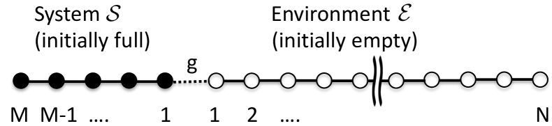
Figure 1: System $\cal S$ coupled to environment $\cal E$. The emptying of the system into the environment leads to Page curve entanglement dynamics.

The total Hilbert space can be decomposed into system and environment sites, ${\cal H}={\cal H}_{\rm sys}\otimes{\cal H}_{\rm env}$, and we will study the entanglement entropy with respect to this decomposition. The total state of system plus environment remains pure for all times and therefore the von Neumann entanglement entropy is given by

$$S_{\rm ent}(t) = -{\rm Tr}_{{\cal H}_{\rm env}}\Big{(}\rho_{\rm env}(t)\ln\rho_{\rm env}(t)\Big{)}$$

$$= -{\rm Tr}_{{\cal H}_{\rm sys}}\Big{(}\rho_{\rm sys}(t)\ln\rho_{\rm sys}(t)\Big{)}$$

with the reduced density operators $\rho_{\rm env}(t)={\rm Tr}_{{\cal H}_{\rm sys}}\,|\Psi(t)\rangle\langle\Psi(t)|$ and $\rho_{\rm sys}(t)={\rm Tr}_{{\cal H}_{\rm env}}\,|\Psi(t)\rangle\langle\Psi(t)|$. The calculation in this paper targets $\rho_{\rm sys}(t)$, for which one has the following intuitive argument why Page curve like behavior is expected: The initial particle imbalance between system $\cal S$ and environment will lead to a decay of the number of particles in the system,

$$m(t)\stackrel{{\scriptstyle\rm def}}{{=}}\langle\Psi(t)|\left(\sum_{i=1}^{M}c^{\dagger}_{i}c_{i}\right)|\Psi(t)\rangle\ .$$ (7)

Initially $m(0)=M$ and after a short transient one expects a constant current $\dot{m}(t)=I$, which can be thought of as the production of a particle-hole pairs at the boundary between system and environment: The holes travels into the system ${\cal S}$ and the particles into the environment ${\cal E}$. Semiclassically particle current and entanglement generation are proportional to one another Calabrese and Cardy (2005), so this leads to linear entanglement growth with a proportionality factor set by the particle current $I$. At late times the particles will be spread out approximately evenly throughout the whole system $\cal S$ and we therefore expect

$$\lim_{t\rightarrow\infty}m(t)=\frac{M^{2}}{M+N}$$ (8)

which vanishes for $N\gg M^{2}$. Notice that strictly speaking the long time limit in (8) requires additional averaging over a suitable time window in order to suppress fluctuations, but this detail plays no role in the sequel. Since the system $\cal S$ empties completely for $N\gg M^{2}$, the quantum state necessarily has product structure at late times

$$|\Psi(t)\rangle=|\Omega_{\rm sys}\rangle\otimes|\Phi_{\rm env}(t)\rangle$$ (9)

and therefore vanishing entanglement. This shows why Page curve entanglement dynamics should be expected for this model.

A more complete picture can be deduced from the observation that any given time one can approximately replace ${\cal H}_{\rm sys}$ with the Hilbert space ${\cal H}_{\rm sys}^{\rm(eff)}$ for $m(t)$ spinless fermions on $M$ lattice sites with

$${\rm dim}\>{\cal H}_{\rm sys}^{\rm(eff)}=\left({M\atop m(t)}\right)\ .$$ (10)

This approximation leads to

$$S_{\rm ent}(t) \leq \ln\,{\rm dim}\>{\cal H}_{\rm sys}^{\rm(eff)}$$

$$\approx m(t)\,\ln\left(\frac{M}{m(t)}\right)+(M-m(t))\,\ln\left(\frac{M}{M-m(t)}\right)$$

where we have used the Stirling approximation. This trivially reproduces the short and long time limit, and is consistent with the entanglement entropy being largest when the system $\cal S$ is half full like for the Page curve. Notice that the underlying argument of replacing ${\cal H}_{\rm sys}$ with ${\cal H}_{\rm sys}^{\rm(eff)}$ is not rigorous since it neglects fluctuations around the expectation number of particles in the system $m(t)$. However, for our model (4) we are able to calculate the entanglement entropy exactly and confirm the intuitive picture developed here.

Numerical solution. The exact calculation of the entanglement entropy relies on the formalism developed by Eisler and Peschel for obtaining the reduced density operator for fermionic or bosonic bilinear Hamiltonians Peschel and Eisler (2009). Applied to our model one has

$$\rho_{\rm sys}=K\,\exp\left(-\sum_{i,j=1}^{M}h_{ij}c^{\dagger}_{i}c_{j}\right)$$ (12)

with the matrix $h$ determined by the one-particle correlation matrix $C_{ij}=\langle c^{\dagger}_{i}\,c_{j}\rangle$ via

$$h=\ln\Big{(}(1-C)/C\Big{)}\ .$$ (13)

The diagonalization of $\rho_{\rm sys}$ yields the von Neumann and all other Renyi entanglement entropies. This formalism also applies for bilinear non-equilibrium problems where the one-particle correlation matrix becomes time-dependent Peschel and Eisler (2009)

$$C_{ij}(t)=\langle\Psi(0)|c^{\dagger}_{i}(t)\,c_{j}(t)|\Psi(0)\rangle\ .$$ (14)

We obtain the time evolved operators $c^{\dagger}_{i}(t)$ and $c_{j}(t)$ from the straightforward exact solution of their Heisenberg equations of motion for the quadratic Hamiltonian $H$ (4), which can easily be done for $N=O(10^{4})$. This has already been utilized extensively in the literature for various other one-dimensional non-equilibrium problems Eisler et al. (2008, 2009); Eisler and Peschel (2012); Capizzi and Eisler (2023).

In this paper we use parameters $N=10^{4},M=25\ldots 75,g=0.35\ldots 0.8,t_{\rm env}=4$ with the overall energy scale set by the hopping in the system $t_{\rm sys}=1$. The main numerical limitations come from particle reflection at the right boundary of the environment chain, which travel back to the system $\cal S$ and prevent a further decay of $m(t)$. This makes it impossible to go to much larger values of $M$ or smaller values of $g$ for given $N=10^{4}$ if one wants to see Page curve physics before finite size effects become noticeable. All values of the hopping matrix elements $t_{\rm env},t_{\rm sys}$ lead to Page curve physics; our choice of $t_{\rm env}=4t_{\rm sys}$ is determined by comparison with an analytical approximation that becomes exact for $t_{\rm env}\gg t_{\rm sys}$ (see next section) and the desire to keep finite size effects under control (because the particles in the environment travel and therefore reflect back faster for larger values of $t_{\rm env}$). Finally the case of a homogeneous chain $t_{\rm sys}=g=t_{\rm env}$ is special since it leads to a logarithmic increase of the entanglement entropy as a function of time vs. the generic linear increase for an inhomogeneous chain (this is well known from the literature Eisler and Peschel (2012)): Since we are interested in the tunneling limit we use $g<t_{\rm sys}$ and stay away from the special homogeneous point.

Analytical solution. The fact that the Hamiltonian (4) is quadratic allows for an analytical solution in the weak coupling limit $g\ll t_{\rm sys},t_{\rm env}$. In a first step one diagonalizes the system Hamiltonian $H_{\rm sys}$, which leads to an equivalent description in terms of single-particle levels $c^{\dagger}_{k},c_{k}$ coupled to the environment,

$$H=\sum_{k=1}^{M}\omega_{k}\,c^{\dagger}_{k}c_{k}+\sum_{k=1}^{M}V_{k}\left(c^{\dagger}_{k}f_{1}+f^{\dagger}_{1}c_{k}\right)+H_{\rm env}\ .$$ (15)

One easily verifies the single particle energies

$$\omega_{k}=-t_{\rm sys}\,\cos\left(\frac{\pi\,k}{M+1}\right)$$ (16)

and hybridization matrix elements

$$V_{k}=g\,\sqrt{\frac{2}{M+1}}\,\sin\left(\frac{\pi\,k}{M+1}\right)$$ (17)

for $k=1..M$ from the analytical solution of a finite chain. In the limit $N\rightarrow\infty$ one can describe the environment via a continuum density of states $\rho(\epsilon)$. Each single particle level $\omega_{k}$ therefore couples predominantly to environment states in an energy interval around $\omega_{k}$ set by the hybridization

$$\Gamma_{k}(\omega_{k})=\pi\rho(\omega_{k})\,V_{k}^{2}.$$ (18)

If the energy difference between adjacent single particle levels is much larger than the hybridization one can think of these single particle levels as being coupled to disjoint environments, see Fig. 2. This condition can be satisfied for sufficiently small coupling $g$ even in the limit $M\rightarrow\infty$ since

$$|\omega_{k+1}-\omega_{k}|\propto\frac{t_{\rm sys}}{M}\gg\Gamma_{k}(\omega_{k})\propto\frac{g^{2}}{M}\rho(\omega_{k})$$ (19)

is true in the weak coupling limit

$$g\ll\sqrt{t_{\rm sys}t_{\rm env}}\ .$$ (20)

Strictly speaking there is a fraction $g^{2}/t_{\rm sys}t_{\rm env}$ of single particle levels close to $k=1$ and $k=M$ where condition (19) does not hold since the dispersion relation (16) becomes flat, but this is negligible in the limit (20).

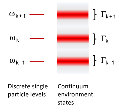
Figure 2: Equivalent description of the model from Fig. 1 in terms of single particle levels coupled to a continuum environment (15). If condition (19) is fulfilled the single particle levels couple to effectively disjoint environments, leading to a model of $M$ disjoint resonant level models (21).

Putting everything together, in the weak coupling limit (20) our model (15) can equivalently be written as a collection of $M$ disjoint resonant level models (RLMs)

$$H^{\rm(RLM)}_{k}=\omega_{k}c^{\dagger}_{k}c_{k}+\sum_{i}V_{k}\left(c^{\dagger}_{k}a_{k,i}+a^{\dagger}_{k,i}c_{k}\right)+\sum_{i}\epsilon_{i}a^{\dagger}_{k,i}a_{k,i}$$ (21)

with hybridization (18)

$$\Gamma_{k}(\epsilon)=\frac{2\pi\rho(\epsilon)\,g^{2}}{M+1}\,\sin^{2}\left(\frac{\pi\,k}{M+1}\right)\ .$$ (22)

The reduced density operator of the system $\rho_{\rm sys}(t)$ is then the direct product of reduced density operators of the $M$ resonant level models

$$\rho_{\rm sys}(t)=\bigotimes_{k=1}^{M}\rho^{(RLM)}_{k}(t)$$ (23)

with

$$\rho^{(RLM)}_{k}(t)=\left(\begin{array}[]{cc}n_{k}(t)&0\\ 0&1-n_{k}(t)\end{array}\right)$$ (24)

where $n_{k}(t)=\langle\Psi(t)|c^{\dagger}_{k}c_{k}|\Psi(t)\rangle$ is the time-dependent occupation number of the impurity orbital. Initially all impurity orbitals are occupied $n_{k}(t=0)=1$ and all bath sites are empty. As a function of time the number of particles in the system is given by $m(t)=\sum_{k=1}^{M}n_{k}(t)$ and the entanglement entropy

$$S_{\rm ent}(t)=-\sum_{k=1}^{M}\left(n_{k}(t)\,\ln n_{k}(t)+(1-n_{k}(t))\,\ln(1-n_{k}(t))\right)\ .$$ (25)

In the wide flat band limit $t_{\rm env}\gg t_{\rm sys}$ we can take the bath density of states as being constant $\rho(\omega_{k})=\rho$ and it is known that the impurity orbital occupation decays purely exponentially in this wide flat band limit Guinea et al. (1985); Langreth and Nordlander (1991)

$$n_{k}(t)=e^{-2\Gamma_{k}t}\ .$$ (26)

For large systems $M\gg 1$ one arrives at

$$\frac{m(\tau)}{M} = \frac{1}{\pi}\int_{0}^{\pi}dk\>n_{k}(\tau)$$ (27)

$$\frac{S_{\rm ent}(\tau)}{M} = -\frac{1}{\pi}\int_{0}^{\pi}dk\>\Big{(}n_{k}(\tau)\,\ln n_{k}(\tau)$$

$$\qquad\qquad+(1-n_{k}(\tau))\,\ln(1-n_{k}(\tau))\Big{)}$$

where

$$n_{k}(\tau)=e^{-\tau\sin^{2}k}$$ (29)

with the dimensionless parameter $\tau=4\pi\rho g^{2}t/M$. Eqs. (27–29) allow us to plot the entanglement entropy as a function of the fractional decay of the system, $S_{\rm ent}=S_{\rm ent}(m/M)$ such that the parameters $g$ and $\rho$ drop out. The resulting curves (shown in the next section) display the universal behavior in the limit $t_{\rm env}\gg t_{\rm sys}\gg g$, $N,M\rightarrow\infty$ while keeping $N\gg M^{2}$.

Entanglement entropy. Starting from the initial state (5) the system $\cal S$ starts to empty as can be seen in Fig. 3 obtained from the numerical solution of the Heisenberg equations of motion. Based on the discussion of (Page curve entanglement dynamics in an analytically solvable model) we therefore expect to see Page curve entanglement dynamics. Fig. 4 is obtained from the numerical solution following the Eisler-Peschel formalism described above and clearly exhibits this behavior: The entanglement entropy increases approximately linearly at early times, reaches its maximum at the Page time $t_{\rm P}\propto M$ and then decays again. The entanglement entropy at the Page time is proportional to the system size, $S_{\rm ent}(t_{\rm P})/M\approx 0.53\pm 0.02$. The proportionality factor is smaller than the Page value $\ln 2$ Page (1993), which is to be expected for a non-interacting system.

Notice that there is no discernible feature at the Page time in observables like the number of particles in the system $m(t)$, Fig. 3. One cannot deduce anything about the bending down of the entanglement entropy from $m(t)$ or the particle current across the boundary $I(t)=\dot{m}(t)$. This also demonstrates the breakdown of the semiclassical connection between particle current and entanglement generation Calabrese and Cardy (2005)

$$\frac{dS_{\rm ent}(t)}{dt}\propto I(t)$$ (30)

beyond the Page time. Due to the highly entangled state that has dynamically developed up to the Page time one can no longer treat particle-hole production at the boundary as leading to a maximally entangled pair that is not entangled with other particles.

Figure 3: Decay of the number of particles $m(t)$ in the system $\cal S$ as a function of time (top: linear scale, bottom: logarithmic scale). The universal behavior after rescaling with $M$ implies a finite current $I(t)=\dot{m}(t)$ across the boundary for large systems $M\rightarrow\infty$ (always keeping the environment even larger $N\gg M^{2}$). Parameters: $t_{\rm env}=4,t_{\rm sys}=1,g=0.5,N=10^{4}$.

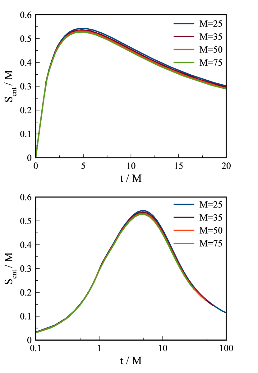
Figure 4: Entanglement entropy as a function of time (top: linear scale, bottom: logarithmic scale). The Page curve behavior is clearly visible with the Page time $t_{\rm P}\propto M$ and $S_{\rm ent}(t_{\rm P})\propto M$. Parameters: $t_{\rm env}=4,t_{\rm sys}=1,g=0.5,N=10^{4}$.

Since the Page time depends on the coupling $g$ between system and environment, a universal way to depict the Page curve in our model is to plot the entanglement entropy as a function of the fraction of particles emitted into the environment, $1-m(t)/M$. The corresponding curves for different values of $g$ are shown in Fig. 5. Specifically, one can observe that the numerical results agree very well with the analytical universal curve from Eqs. (27–29) (dashed line) for small values of $g$. The remaining deviations at late times are due to numerical limitations for the ratio $t_{\rm env}/t_{\rm sys}$ which one cannot choose much larger for $N=10^{4}$.

Page curve behavior is also visible in all Renyi entropies

$$S^{(q)}=\frac{1}{1-q}\,\ln{\rm Tr}_{{\cal H}_{\rm sys}}\left(\rho_{\rm sys}\right)^{q}\ .$$ (31)

This is depicted in Fig. 6 for the purity $S^{(2)}(t)$ and in Fig. 7 for the min-entropy $S^{(q=\infty)}(t)$. For larger values of $q$ the bending down at the Page time becomes more sudden with little indication of it at earlier times, see Fig. 7.

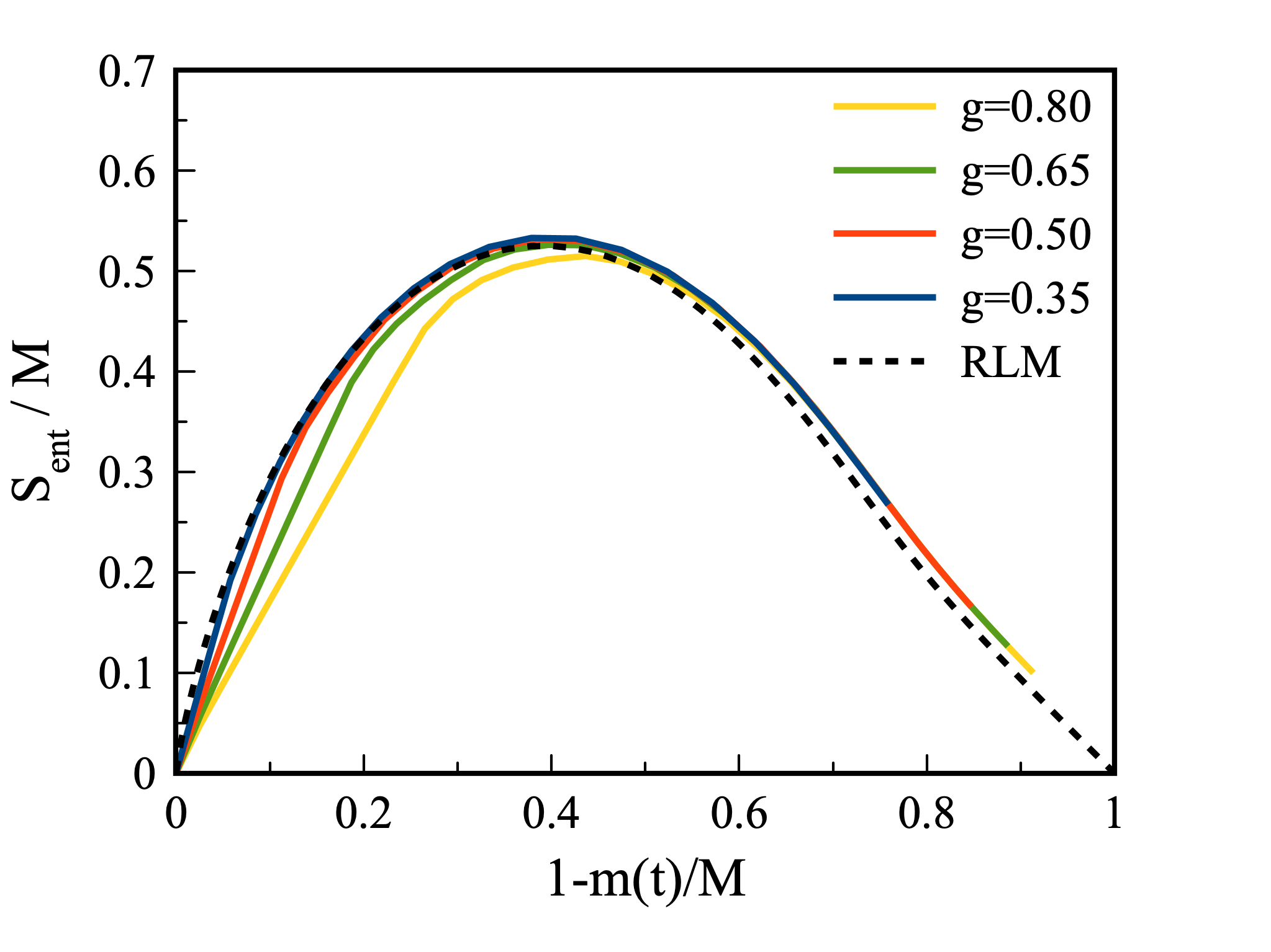
Figure 5: Entanglement entropy as a function of the fraction of particles that have been emitted into the environment for various system-environment couplings $g$ (3). The curves become universal in the weak-coupling limit $g\rightarrow 0$ and approach the analytical result from the disjoint resonant level model description (dashed line). Parameters: $t_{\rm env}=4,t_{\rm sys}=1,M=50,N=10^{4}$.

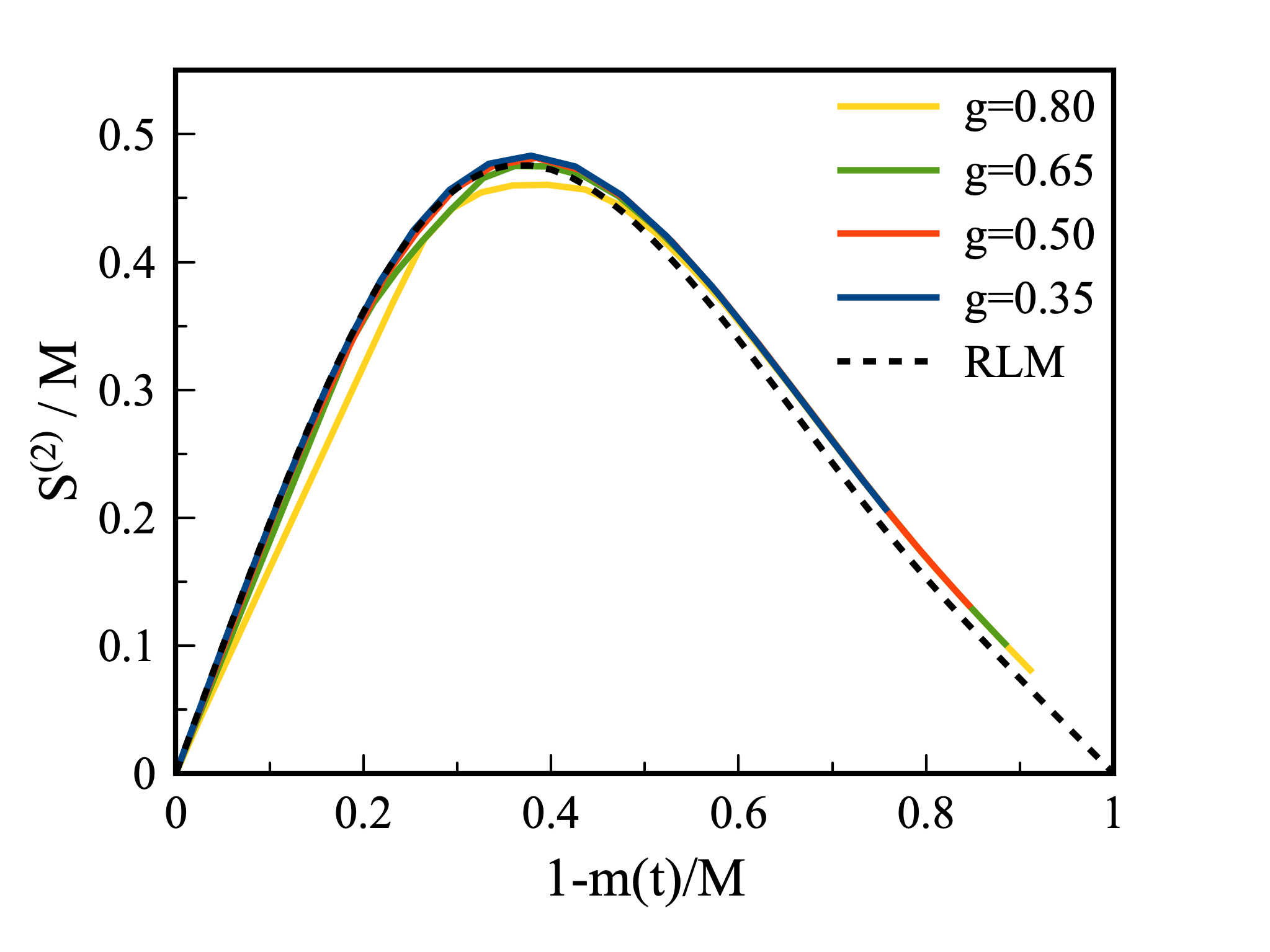
Figure 6: Purity $S^{(2)}$ as a function of the fraction of particles that have been emitted into the environment for various system-environment couplings $g$. The dashed line is the analytical result from the disjoint resonant level model description. Parameters: $t_{\rm env}=4,t_{\rm sys}=1,M=50,N=10^{4}$.

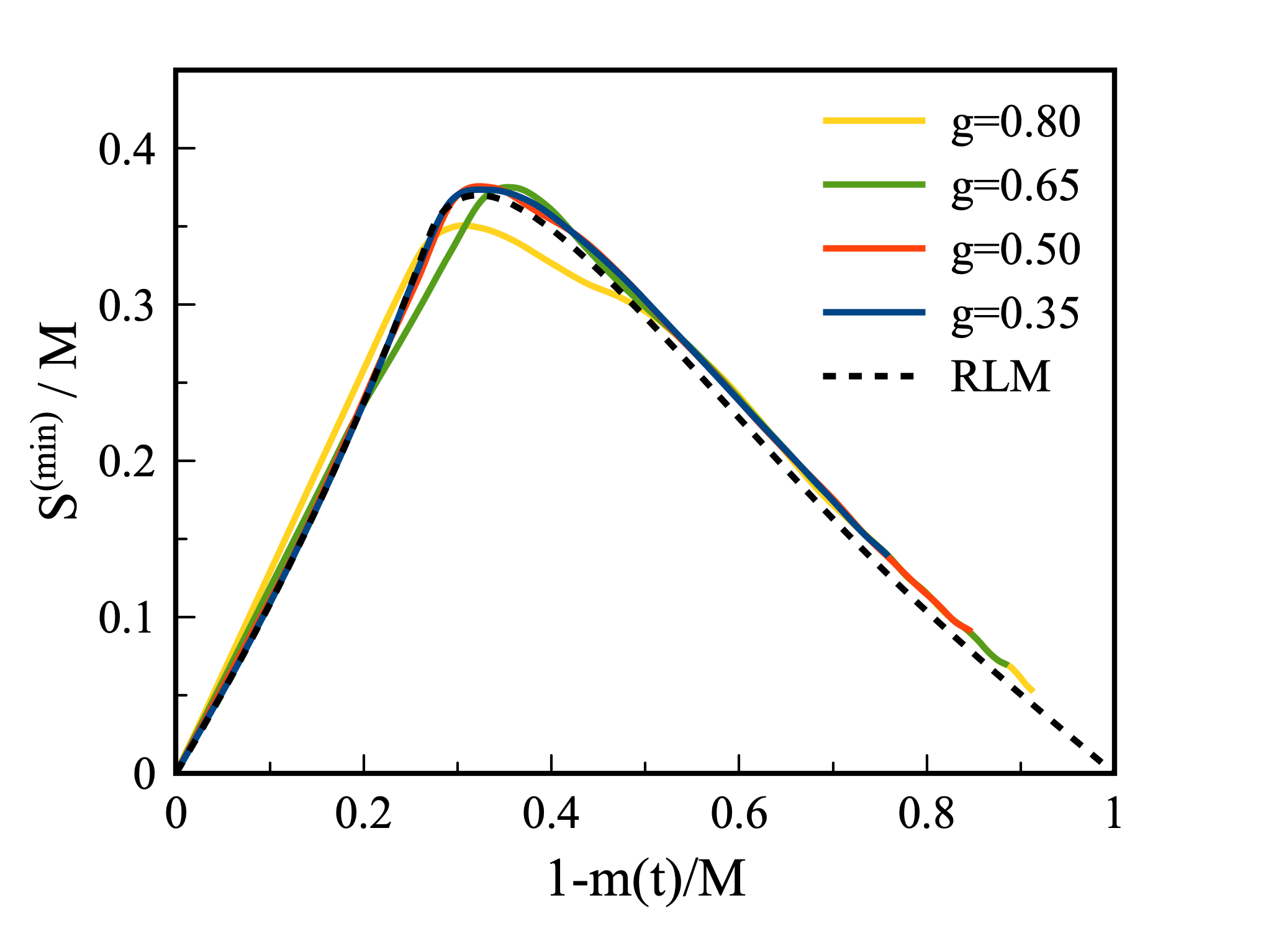
Figure 7: Min-entropy $S^{({\rm min})}$ as a function of the fraction of particles that have been emitted into the environment for various system-environment couplings $g$. The dashed line is the analytical result from the disjoint resonant level model description. Parameters: $t_{\rm env}=4,t_{\rm sys}=1,M=50,N=10^{4}$.

Low energy variance states. Behavior related to the Page curve can also be seen in the energy variance of the environment Hamiltonian (2),

$$\Delta H_{\rm env}^{2}(t)\stackrel{{\scriptstyle\rm def}}{{=}}\langle\big{(}H_{\rm env}-\langle H_{\rm env}\rangle_{t}\big{)}^{2}\rangle_{t}\ .$$ (32)

Here $\langle\ldots\rangle_{t}$ indicates that the expectation value is taken with respect to the state at time $t$, $\langle O\rangle_{t}=\langle\Psi(t)|O|\Psi(t)\rangle$. $\Delta H_{\rm env}(t)$ is indicative of the number of eigenstates that contribute to the state in the environment. It can only vanish if the environment is in an eigenstate of $H_{\rm env}$. Generically, for independent unentangled particles the variance $\Delta H_{\rm env}^{2}$ is proportional to their number. Interestingly, this is very different in our model where one generates a low variance state with $\Delta H_{\rm env}^{2}(t)\propto O(M^{0})$ for $t\rightarrow\infty$. The argument for this is similar to the one for the Page curve: The variance of the full Hamiltonian $H=H_{\rm sys}+H_{\rm c}+H_{\rm env}$ is time invariant and therefore given by its initial value, to which only the boundary coupling term contributes,

$$\Delta H^{2}(t) = \Delta H^{2}(t=0)=\langle\big{(}H_{\rm c}-\langle H_{\rm c}\rangle_{0}\big{)}^{2}\rangle_{0}$$ (33)

$$= t_{\rm sys}^{2}\ .$$

Some straightforward manipulation yields

$$\Delta H_{\rm env}^{2}(t) = \Delta H^{2}(t)$$ (34)

$$+\Delta H_{A}^{2}(t)+2\langle H\rangle_{0}\,\langle H_{A}\rangle_{t}$$

$$-\langle\big{\{}H,e^{iHt}H_{A}e^{-iHt}\big{\}}\rangle_{0}\ ,$$

where $H_{A}=H_{\rm sys}+H_{\rm c}$. Since the system $\cal S$ empties asympotically for large environments $N\gg M^{2}$, the second and third line of (34) vanish for $t\rightarrow\infty$ and hence

$$\lim_{t\rightarrow\infty}\Delta H_{\rm env}^{2}(t)=\Delta H^{2}(t)=t_{\rm sys}^{2}\ .$$ (35)

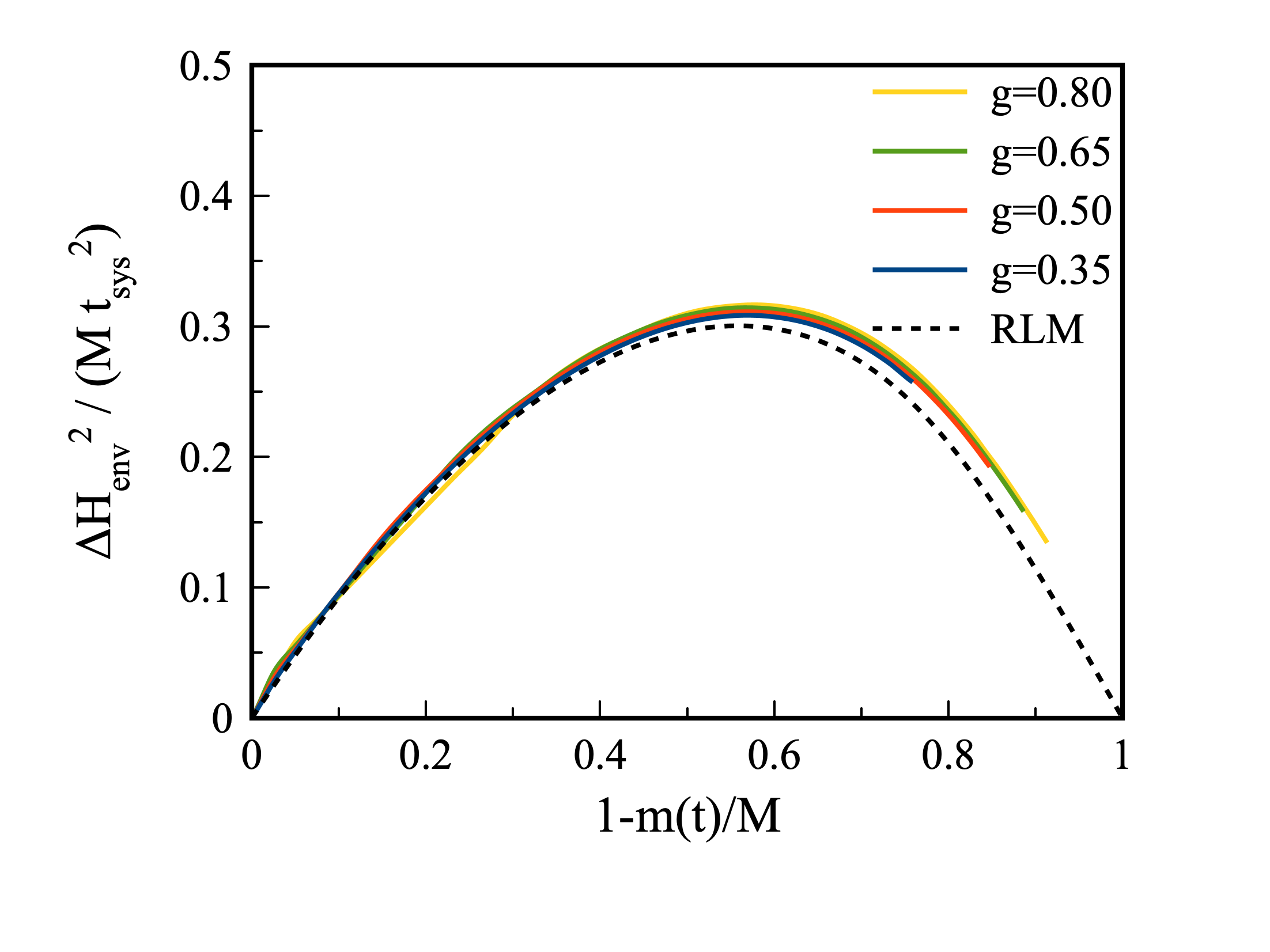
Figure 8: Energy variance with respect to the environment Hamiltonian (2) as a function of the fraction of particles that have been emitted into the environment for various system-environment couplings $g$. The dashed line is the analytical result from the disjoint resonant level model description with a limiting value $\lim_{t\rightarrow\infty}\Delta H_{\rm env}^{2}(t)=O(M^{0})$ corresponding to the generation of a low energy variance state in the environment. Parameters: $t_{\rm env}=4,t_{\rm sys}=1,M=50,N=10^{4}$.

Fig. 8 depicts the scaled energy variance $\Delta H_{\rm env}^{2}(t)/M$ for various couplings $g$ from the numerical solution of (34). One observes that the energy variance $\Delta H_{\rm env}^{2}(t)$ reaches it largest value proportional to system size $M$ when about half the number of particles has been emitted into the environment, after which the energy variance becomes smaller again. For weak system-environment coupling $g$ one can also the mapping to the model of disjoint resonant level models (Fig. 2),

$$\Delta H_{\rm env}^{2}(t)=\sum_{k=1}^{M}\left(\Delta H_{k}^{\rm(RLM)}\right)^{2}(t)$$ (36)

with

$$\left(\Delta H_{k}^{\rm(RLM)}\right)^{2}(t)=\omega_{k}^{2}\,n_{k}(t)\,(1-n_{k}(t))+O(V_{k}^{2})\ .$$ (37)

For $M\gg 1$ this gives

$$\frac{\Delta H_{\rm env}^{2}(\tau)}{M}=\frac{t_{\rm sys}^{2}}{\pi}\int_{0}^{\pi}dk\,\cos^{2}(k)\,n_{k}(\tau)\,(1-n_{k}(\tau))$$ (38)

with $n_{k}(\tau)$ from (29). The resulting curve is depicted in Fig. 8: It agrees very well with the numerical solution and shows the generation of a low variance state in the environment as the system $\cal S$ continues to emit particles into the environment after the Page time.

Interpretation and generalizations. From the point of view of an observer in the system $\cal S$ the dynamical behavior of the entanglement or the energy variance is not surprising. Initially, system plus environment are in an unentangled product state (5). The process of emitting particles into the environment generates a complicated state in the system $\cal S$ that is entangled with the environment, but ultimately this process continues for so long that the system $\cal S$ is driven into a very small effective Hilbert space ${\cal H}^{\rm(eff)}_{\rm sys}(t\rightarrow\infty)$. Therefore entanglement and environment energy variance are forced to decrease again since the asymptotic small effective Hilbert space does not permit larger values. Fig. 9 gives a schematic picture of this process. Notice that in our model we have ${\rm dim}\,{\cal H}^{\rm(eff)}_{\rm sys}(t\rightarrow\infty)=1$ for $N\gg M^{2}$ and hence $S_{\rm ent}(t\rightarrow\infty)=0$. However, even for smaller ratios $N/M^{2}$ one can expect to see Page curve behavior in the sense that the entanglement entropy decreases after the Page time, albeit it will not decrease all the way to zero if ${\rm dim}\,{\cal H}^{\rm(eff)}_{\rm sys}(t\rightarrow\infty)>1$. Such finite size behavior is depicted in Fig. 10 and would be important for experimental realizations where one might not achieve $N/M^{2}\rightarrow 0$. Likewise the observations made here will carry over to interacting systems or higher dimensions since the mechanism in Fig. 9 is universal (however, then one is numerically limited to much smaller models).

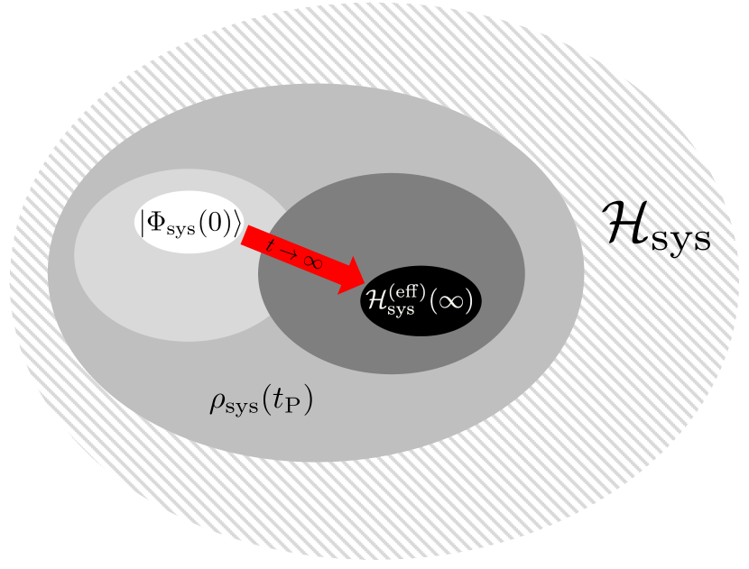
Figure 9: Schematic picture of the dynamics leading to the Page curve. The full colored regions depict the size of the effective Hilbert space that is necessary in order to represent $\rho_{\rm sys}(t)$ at different times $t$. Darker colors correspond to later times. In our model eventually the particle current forces the system $\cal S$ into a small effective Hilbert space ${\cal H}^{\rm(eff)}_{\rm sys}(\infty)$. Although the state $\rho_{\rm env}(t)$ in the environment at late times has a complicated non-local structure, its von Neumann entropy is bounded by $\ln{\rm dim}{\cal H}^{\rm(eff)}_{\rm sys}(\infty)$. Similar scenarios could also be realized in other models by forcing mechanisms like energy or spin currents.

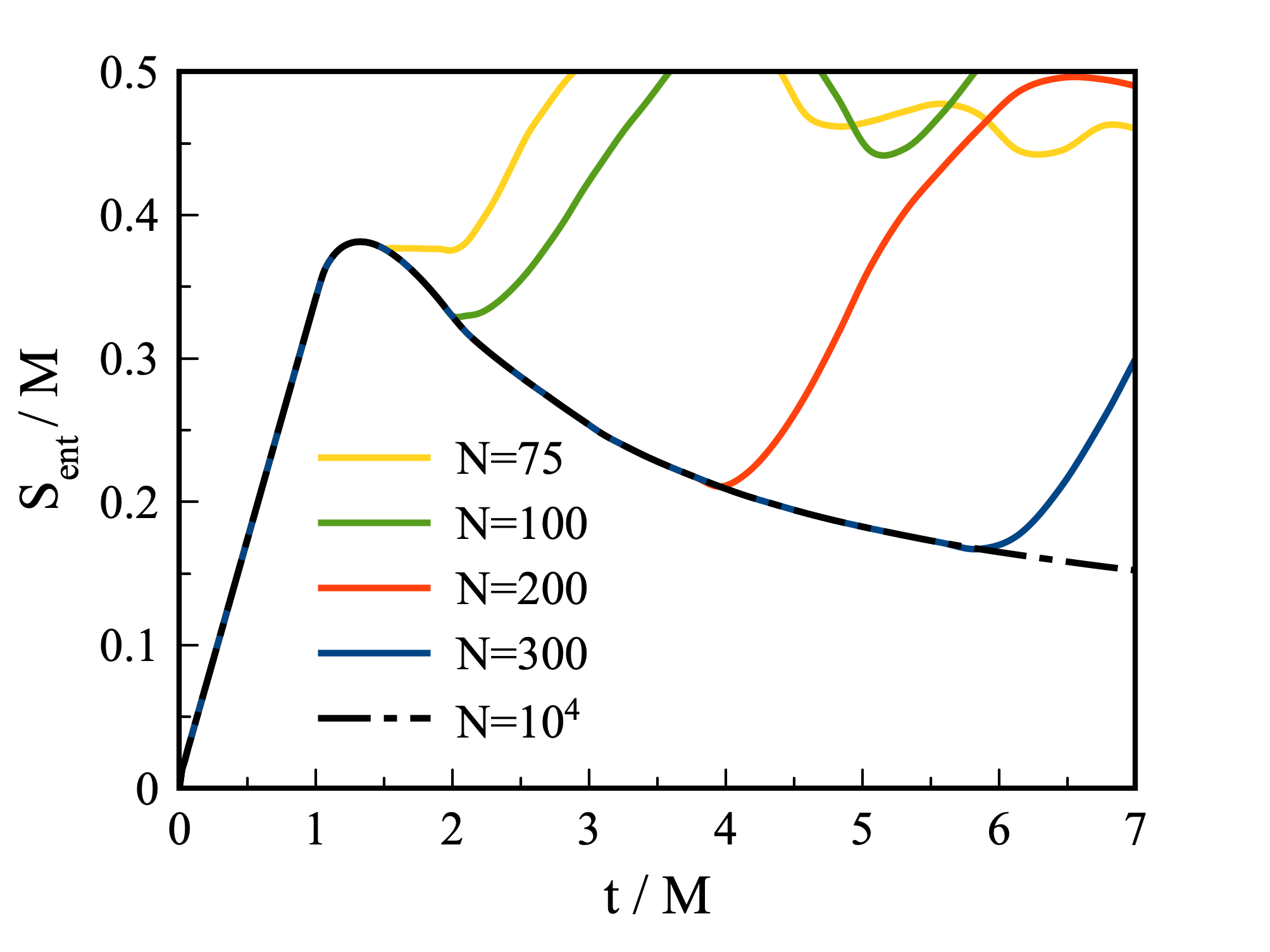
Figure 10: Entanglement entropy as a function of time for varying environment sizes $N$. The system size is $M=50$, other parameters $t_{\rm env}=t_{\rm sys}=1,g=0.65$. For this set of parameters the decrease of entropy after the Page time starts to set in for $N/M\approx 1.5$ and is clearly noticeable once $N/M\gtrsim 4$. The eventual increase of the entanglement entropy for even longer times (as the curves start to deviate from the $N=10^{4}$ curve) is due to the system not emptying out completely into the environment and particles being reflected at the right boundary of the environment.

While the decrease of the entanglement entropy after the Page time $t_{\rm P}$ can easily be understood from the system point of view, a non-omniscient observer in the environment will find it puzzling: The environment keeps absorbing particles that have the curious property of reducing its entanglement entropy and decreasing the energy variance. This behavior is reminiscent of gas particles carefully reassembling themselves in one half of a gas cylinder that they were initially released from. Of course one can always achieve a decrease of entropy in time-reversal invariant systems by first running time backwards to $-t_{0}<0$ from an initially ordered state $|\Psi(0)\rangle$, and then using this state $|\Psi(-t_{0})\rangle$ as the starting point for forward time evolution: In the time interval $[-t_{0},0]$ the entropy then has to decrease. However, this decrease as a function of time is very unstable for generic systems and even small perturbations will drive the entropy up again in the time interval $[-t_{0},0]$. This apparent contradiction between the second law of thermodynamics and microscopic time-reversal invariance was at the center of the Boltzmann-Loschmidt debate, and has been resolved by the understanding of chaotic behavior in generic many-particle systems. Another possibility to generate a decreasing entanglement entropy exists in integrable models with (nearly) linear dispersion relation: For appropriately chosen finite environment sizes one can achieve a refocusing of the quasiparticles that leads to periodic dips of the entanglement entropy Surace et al. (2020).

In contrast to such fine-tuned and highly sensitive scenarios with a decreasing entropy, models that follow Fig. 9 like the exactly solvable model analyzed in this paper show a robust decrease of the entanglement entropy after the Page time. Notice that at the Page time the entanglement entropy can be made arbitrarily large by increasing $M$. Even time-dependent perturbations to the system or the environment will not change the qualitative behavior of decreasing entanglement entropy after the Page time as long as the system $\cal S$ empties into the environment, i.e. as long as Fig. 9 remains applicable. An observer limited to the environment with no knowledge of the full initial state would conclude from such a robust decrease of the entanglement entropy that one is watching a movie running backwards. The dynamical buildup of long range entanglement between ${\cal H}_{\rm sys}$ and ${\cal H}_{\rm env}$ up to the Page time is ultimately responsible for the robust Page curve behavior: Particles emitted into the environment after the Page time carry entanglement across the boundary leading to the bending down of the Page curve. This behavior is robust as long as time evolution is unitary and one does not couple to additional external degrees of freedom.

Finally, it should be emphasized that one cannot make similarly general statements about a bending down of coarse-grained entropies based on Fig. 9 since this will depend on the specific coarse-graining procedure employed Almheiri et al. (2021).

Summary. This paper introduced an exactly solvable model as an example for the general scenario depicted in Fig. 9 resulting in a Page curve. Unitary time evolution leads to an increase of the entanglement entropy until the Page time consistent with the semiclassical propotionality between particle current and entanglement generation (30). At the Page time the entanglement entropy can be arbitrarily large since it is proportional to the number of particles $M$ initially in the system ${\cal S}$. Beyond the Page time the entanglement entropy decreases again and this semiclassical picture breaks down. The scenario depicted in Fig. 9 generates entanglement dynamics different from the saturation at the volume law scenario commonly discussed in the literature without the need for any fine tuning. We have therefore constructed a solvable model that illustrates Polchinski’s burning piece of coal Polchinski (2016): The early photons are entangled with the remaining coal, but when the coal has burned completely the outgoing photons must be in a pure state (assuming the coal was initially in a pure state). While this is fundamentally different from a black hole due to the lack of an event horizon Polchinski (2016), one can make two observations in this exactly solvable model that have analogues in black hole physics: i) The semiclassical picture breaks down for a subtle quantity like the entanglement entropy once the system $\cal S$ in ${\cal H}_{\rm sys}$ has evolved to a sufficiently complex state at the Page time Akers et al. . ii) At early times there is little or no indication of the eventual bending down of the Page curve, see Figs. 4-7.

One related interesting property of the state in the environment is that its energy variance decreases after the Page time $t_{\rm P}$ (Fig. 8), corresponding to fewer eigenstates of $H_{\rm env}$ contributing to it. Asypmotically for $t\gg t_{\rm P}$ the energy variance $\Delta H_{\rm env}^{2}$ becomes independent of the number of particles $M$ in the environment (35), which is different from the usual linear dependence on $M$ for independently injected particles into ${\cal H}_{\rm env}$. Such states with reduced energy uncertainty at nonzero excitation energy could be of interest experimentally.

Acknowledgments. I thank R. Jha and L. Tagliacozzo for valuable discussions. This work is funded by the Deutsche Forschungsgemeinschaft (DFG, German Research Foundation)-217133147/SFB 1073 (Project No. B07). It was performed in part at the Aspen Center for Physics, which is supported by National Science Foundation grant PHY-2210452, and at the Kavli Institute for Theoretical Physics (KITP), supported by grants NSF PHY-1748958 and PHY-2309135, whose hospitality is gratefully acknowledged.

References

- Eisert et al. (2010) J. Eisert, M. Cramer, and M. B. Plenio, “Colloquium: Area laws for the entanglement entropy,” Rev. Mod. Phys. 82, 277–306 (2010).
- Schollwöck (2011) Ulrich Schollwöck, “The density-matrix renormalization group in the age of matrix product states,” Annals of Physics 326, 96–192 (2011), january 2011 Special Issue.
- Ryu and Takayanagi (2006) Shinsei Ryu and Tadashi Takayanagi, “Holographic derivation of entanglement entropy from the anti–de sitter space/conformal field theory correspondence,” Phys. Rev. Lett. 96, 181602 (2006).
- Calabrese and Cardy (2005) Pasquale Calabrese and John Cardy, “Evolution of entanglement entropy in one-dimensional systems,” Journal of Statistical Mechanics: Theory and Experiment 2005, P04010 (2005).
- Ho and Abanin (2017) Wen Wei Ho and Dmitry A. Abanin, “Entanglement dynamics in quantum many-body systems,” Phys. Rev. B 95, 094302 (2017).
- Kim and Huse (2013) Hyungwon Kim and David A. Huse, “Ballistic spreading of entanglement in a diffusive nonintegrable system,” Phys. Rev. Lett. 111, 127205 (2013).
- Hawking (1975) S. W. Hawking, “Particle creation by black holes,” Communications in Mathematical Physics 43, 199 (1975).
- Page (1993) Don N. Page, “Information in black hole radiation,” Phys. Rev. Lett. 71, 3743–3746 (1993).
- Page (2013) Don N. Page, “Time dependence of hawking radiation entropy,” Journal of Cosmology and Astroparticle Physics 2013, 028 (2013).
- Mathur (2009) Samir D. Mathur, “The information paradox: a pedagogical introduction,” Classical and Quantum Gravity 26, 224001 (2009).
- Almheiri et al. (2021) Ahmed Almheiri, Thomas Hartman, Juan Maldacena, Edgar Shaghoulian, and Amirhossein Tajdini, “The entropy of hawking radiation,” Rev. Mod. Phys. 93, 035002 (2021).
- Hawking (1976) S. W. Hawking, “Breakdown of predictability in gravitational collapse,” Phys. Rev. D 14, 2460–2473 (1976).
- Papadodimas and Raju (2013) K. Papadodimas and S. Raju, “An infalling observer in ads/cft,” J. High Energ. Phys. 2013, 212 (2013).
- Lunin and Mathur (2002) Oleg Lunin and Samir D. Mathur, “Ads/cft duality and the black hole information paradox,” Nuclear Physics B 623, 342–394 (2002).
- Almheiri et al. (2013) A. Almheiri, D. Marolf, J. Polchinski, and J. Scully, “Black holes: complementarity or firewalls?” J. High Energ. Phys. 2013, 62 (2013).
- Almheiri et al. (2019) A. Almheiri, N. Engelhardt, D. Marolf, and H. Maxfield, “The entropy of bulk quantum fields and the entanglement wedge of an evaporating black hole,” J. High Energ. Phys. 2019, 63 (2019).
- Penington et al. (2022) G. Penington, S.H. Shenker, D. Stanford, and Z. Yang, “Replica wormholes and the black hole interior,” J. High Energ. Phys. 2022, 205 (2022).
- (18) C. Akers, N. Engelhardt, D. Harlow, G. Penington, and S. Vardhan, “The black hole interior from non-isometric codes and complexity,” Preprint arXiv:2207.06536 .
- Liu and Vardhan (2021) Hong Liu and Shreya Vardhan, “A dynamical mechanism for the Page curve from quantum chaos,” Journal of High Energy Physics 2021, 88 (2021).
- Lau et al. (2022) Pak Hang Chris Lau, Toshifumi Noumi, Yuhei Takii, and Kotaro Tamaoka, “Page curve and symmetries,” Journal of High Energy Physics 2022, 15 (2022).
- Chen et al. (2020a) Yiming Chen, Xiao-Liang Qi, and Pengfei Zhang, “Replica wormhole and information retrieval in the SYK model coupled to Majorana chains,” Journal of High Energy Physics 2020, 121 (2020a).
- Chen et al. (2020b) H. Z. Chen, R. C. Myers, D. Neuenfeld, I. A. Reyesc, , and J. Sandora, “Quantum extremal islands made easy. part ii. black holes on the brane,” J. High Energ. Phys. , 25 (2020b).
- Geng et al. (2021) H. Geng, S. Lüst, R. K. Mishra, and D. Wakeham, “Holographic bcfts and communicating black holes,” J. High Energ. Phys. 2021, 3 (2021).
- Geng et al. (2022) H. Geng, L. Randall, and E. Swanson, “Bcft in a black hole background: an analytical holographic model,” J. High Energ. Phys. , 56 (2022).
- Heidrich-Meisner et al. (2009) F. Heidrich-Meisner, S. R. Manmana, M. Rigol, A. Muramatsu, A. E. Feiguin, and E. Dagotto, “Quantum distillation: Dynamical generation of low-entropy states of strongly correlated fermions in an optical lattice,” Phys. Rev. A 80, 041603 (2009).
- Peschel and Eisler (2009) Ingo Peschel and Viktor Eisler, “Reduced density matrices and entanglement entropy in free lattice models,” Journal of Physics A: Mathematical and Theoretical 42, 504003 (2009).
- Eisler et al. (2008) V Eisler, D Karevski, T Platini, and I Peschel, “Entanglement evolution after connecting finite to infinite quantum chains,” Journal of Statistical Mechanics: Theory and Experiment 2008, P01023 (2008).
- Eisler et al. (2009) Viktor Eisler, Ferenc Iglói, and Ingo Peschel, “Entanglement in spin chains with gradients,” Journal of Statistical Mechanics: Theory and Experiment 2009, P02011 (2009).
- Eisler and Peschel (2012) Viktor Eisler and Ingo Peschel, “On entanglement evolution across defects in critical chains,” Europhysics Letters 99, 20001 (2012).
- Capizzi and Eisler (2023) Luca Capizzi and Viktor Eisler, “Entanglement evolution after a global quench across a conformal defect,” SciPost Phys. 14, 070 (2023).
- Guinea et al. (1985) F. Guinea, V Hakim, and A Muramatsu, “Bosonization of a two-level system with dissipation,” Physical Review Letters 32, 4410 – 4418 (1985).
- Langreth and Nordlander (1991) David C. Langreth and P. Nordlander, “Derivation of a master equation for charge-transfer processes in atom-surface collisions,” Physical Review B 43, 2541–2557 (1991).
- Surace et al. (2020) Jacopo Surace, Luca Tagliacozzo, and Erik Tonni, “Operator content of entanglement spectra in the transverse field ising chain after global quenches,” Phys. Rev. B 101, 241107 (2020).
- Polchinski (2016) Joseph Polchinski, “The black hole information problem,” in New Frontiers in Fields and Strings (World Scientific, 2016).