Compelling ReLU Network Initialization and Training to
Leverage Exponential Scaling with Depth
Abstract
A neural network with ReLU activations may be viewed as a composition of piecewise linear functions. For such networks, the number of distinct linear regions expressed over the input domain has the potential to scale exponentially with depth, but it is not expected to do so when the initial parameters are chosen randomly. This poor scaling can necessitate the use of overly large models to approximate even simple functions. To address this issue, we introduce a novel training strategy: we first reparameterize the network weights in a manner that forces an exponential number of activation patterns to manifest. Training first on these new parameters provides an initial solution that can later be refined by updating the underlying model weights. This approach allows us to produce function approximations that are several orders of magnitude better than their randomly initialized counterparts.
1 Introduction
Beyond complementary advances in areas like hardware, storage, and networking, the success of neural networks is primarily due to their ability to efficiently capture and represent nonlinear functions (Gibou et al., 2019). In a neural network, the goal of an activation function is to introduce nonlinearity between the network’s layers so that the network does not simplify to a single linear function. The rectified linear unit (ReLU) has a unique interpretation in this regard. Since it can only deactivate a neuron or apply the identity operation, it transforms a series of matrix multiplications into a multi-linear function; each possible configuration of active and inactive neurons can produce a unique linear transformation over a region of input space. Thus, for a ReLU network, the number of activation patterns and their corresponding linear regions can theoretically scale exponentially with the depth of the network111The reader is referred to Chmielewski-Anders (2020) for definitions of linear regions, activation patterns, and activation regions.. Hence deep architectures may outperform shallow ones.
Surprisingly, though, a sophisticated theory of how to best encode functions into ReLU networks is lacking, and in practice, adding depth is often observed to help less than one might expect from this exponential intuition. Lacking more advanced theory, practitioners typically use random parameter initialization and gradient descent, the drawbacks of which often lead to extremely inefficient solutions. Hanin & Rolnick (2019) show a rather disappointing bound pertaining to randomly initialized networks: they prove that the average number of linear regions formed upon initialization is entirely independent of the configuration of the neurons, so depth is not properly utilized. They observed that gradient descent has a difficult time creating new activation regions and that their bounds approximately held after training. As we will discuss later, the number of linear regions is not actually a model property that gradient descent can directly optimize. Gradient descent is also prone to redundancy; Frankle & Carbin (2019) show how up to 90% of neurons may ultimately be eliminated from a network without significantly degrading accuracy.
The present work aims to begin eliminating these inefficiencies, starting in a simple one-dimensional setting. Drawing inspiration from existing theoretical ReLU constructions, our novel contributions include a special reparameterization of a ReLU network that forces it to maintain an exponential number of activation patterns over the input domain. We then demonstrate a novel pretraining strategy, which uses these derived parameters before manipulating the underlying matrix weights. This allows the network to discover solutions that are more accurate and unlikely to be found otherwise. Initializing with an exponential number of regions is already improbable, but our pretraining strategy forcibly retains these regions where unassisted gradient descent would otherwise make short-sighted optimizations that discard them. Thus, our pretraining strategy leaves minimal work up to unassisted gradient descent, which then does not have to discover exponentially many new regions. Our results demonstrate that minimizing the reliance of network training on unassisted gradient descent can reliably produce error values orders of magnitude lower than a traditionally trained network of equal size. Although the preliminary results in this theoretical study pertain to one-dimensional convex functions, the paper concludes with our views on extending these theoretical exponential benefits for ReLU networks to arbitrary smooth functions with arbitrary dimensionality, which would have significant practical utility.
2 Related Work
This work is primarily concerned with novel training methodology, but it also possesses a significant approximation theoretic component. Our work can be viewed as a first step towards generalizing the approximation to we review in this section. The reparameterization we employ modifies this method to become trainable to represent other convex one-dimensional functions and then converts that result back into a matrix representation.
2.1 Related Work in Approximation
Infinitely wide neural networks are known to be universal function approximators, even with only one hidden layer (Hornik et al., 1989; Cybenko, 1989). Infinitely deep networks of fixed width are universal approximators as well (Lu et al., 2017; Hanin, 2019). In finite cases, the trade-off between width and depth is often studied in assessing the capability of a network to approximate a function.
Notably, there exist functions that can be represented with a sub-exponential number of neurons in a deep architecture, yet which require an exponential number of neurons in a wide and shallow architecture. For example, Telgarsky (2015) shows that deep neural networks with ReLU activations on a one-dimensional input are able to generate symmetric triangle waves with an exponential number of linear segments (shown in Figure 1 as the ReLU network ). This network functions as follows: each layer takes a one-dimensional input on , and outputs a one-dimensional signal also on . The function they produce in isolation is a single symmetric triangle. Together in a network, each layer feeds its output to the next, performing function composition. Since each layer converts lines from 0 to 1 into triangles, it doubles the number of linear segments in its input signal, exponentially scaling with depth.
The novel reparameterization strategy contributed by the present work aims to extend this idea, compelling ReLU networks to compose rapidly oscillating triangular signals. The key insight is that instead of expressing each layer by its weights, we can train the location on of a triangular function’s peak and then set that layer’s weights accordingly. Composing the layers together will create a variety of dilated triangular waveforms that the network can use in its approximations. We emphasize that while the (Telgarsky, 2015) approximation uses fixed symmetric triangles and is not trainable, a key insight of our work is to instead leverage non-symmetric triangles, which yields trainable parameters (one per triangle).
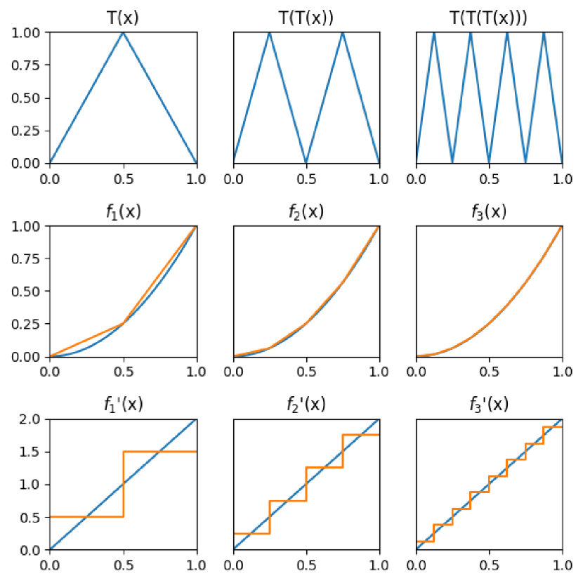
Nonetheless, with only symmetric triangle waves, Yarotsky (2017) and Liang & Srikant (2016) demonstrate the ability to construct on with exponential accuracy. To produce their approximation, one begins with , then computes , , , and so forth, as pictured in Figure 1. As these successive approximations are computed, Figure 1 plots their convergence to , as well as the convergence of the derivatives. We note that these prior papers explicitly focus on approximating using symmetric triangle waves, unlike the present work, which is more general (although those papers leverage their approximation to also indirectly build approximations of other functions).
The techniques of Yarotsky (2017) and Liang & Srikant (2016) seem to touch on something fundamental regarding how ReLU networks can approximate functions: even though individual neuron outputs may be jagged (e.g., Figure 1, top row), an appropriate infinite sum of them (e.g., ) may still be differentiable. Moreover, the derivative of the approximation produced by this technique also converges to the true solution in the limit. Therefore, inspired by the exponential accuracy of this technique, we place a particular emphasis on investigating the relative importance of differentiability throughout the paper. We will argue with numerical evidence that enforcing convergence of the derivative can be a good protection against overfitting in ReLU networks.
One of the appealing properties of neural networks is that they are highly modular. The approximation is used by other theoretical works as a building block to guarantee exponential convergence rates in more complex systems. One possible use case is to construct a multiplication gate. Perekrestenko et al. (2018) does so via the identity . The squared terms can all be moved to one side, expressing the product as a linear combination of squared terms. They then further assemble these multiplication gates into an interpolating polynomial, which can have an exponentially decreasing error when the interpolation points are chosen to be the Chebyshev nodes. Polynomial interpolation does not scale well into high dimensions, so this and papers with similar approaches will usually come with restrictions that limit function complexity: Wang et al. (2018) requires low input dimension, Montanelli et al. (2020) uses band limiting, and Chen et al. (2019) approximates low dimensional manifolds. In light of these prior papers, the present work revisits the approximation, seeking a generalization that can avoid the limitations of these works. Replacing with a more flexible class of functions may produce a suitable building block for techniques that can bypass polynomial interpolation.
Lastly, other works focus on showing how ReLU networks can encode and subsequently surpass traditional approximation methods (Lu et al., 2021; Daubechies et al., 2022). Interestingly, certain fundamental themes from above like composition, triangles, or squaring are still present. One other interesting comparison of the present work is to Ivanova & Kubat (1995), which uses decision trees as a means to initialize neural networks. It is a sigmoid/classification analogy to this work, but rather than an attempting to improve neural networks with decision trees, it is an attempt to improve decision trees with neural networks.
2.2 Related Work in Initialization
Our work seeks to improve network initialization by making use of explicit theoretical constructs. This stands in sharp contrast the current standard approach, which treats neurons homogeneously. Two popular initialization methods implemented in PyTorch are the Kaiming (He et al., 2015) and Xavier initialization (Glorot & Bengio, 2010). They use weight values that are sampled from distributions defined by the input and output dimension of each layer. Aside from sub-optimal approximation power associated with random weights, a common issue is that an entire ReLU network can collapse into outputting a constant value at initialization. This is referred to as the dying ReLU phenomenon (Qi et al., 2024; Nag et al., 2023). It occurs when the initial weights and biases cause every neuron in a particular layer to output a negative value. The ReLU activation then sets the output of that layer to 0, blocking any gradient updates. Worryingly, as depth goes to infinity, the dying ReLU phenomenon becomes increasingly likely (Lu et al., 2020). Several papers propose solutions: Shin & Karniadakis (2020) use a data-dependent initialization, while Singh & Sreejith (2021) introduce an alternate weight distribution called RAAI that can reduce the likelihood of the issue and increase training speed. We observed during our experiments that RAAI greatly reduces, but does not eliminate the likelihood of dying ReLU. Our approach enforces a specific network structure that does not collapse in this manner.
3 Compositional Networks
We begin by discussing how to deliberately architect the weights of a 4 neuron wide, depth ReLU network to induce a number of linear segments exponential in . Throughout the paper, we refer to these as compositional networks. First we will introduce their mathematical form, and then we will discuss how to encode them as ReLU networks.
We define a triangle function as
where . This produces a triangular shape with a peak at and both endpoints at . Each layer in a compositional network in isolation would compute these if directly fed the input signal. Its derivatives are the piecewise linear functions:
| (1) |
In a compositional network, the layers feed into each other. This composes triangle functions into triangle waves:
| (2) |
The output of a compositional network will be a weighted sum over the triangle waves formed at each layer. Assuming the network to be infinitely deep we have
| (3) |
where are scaling coefficients on each of the composed triangular waveforms .
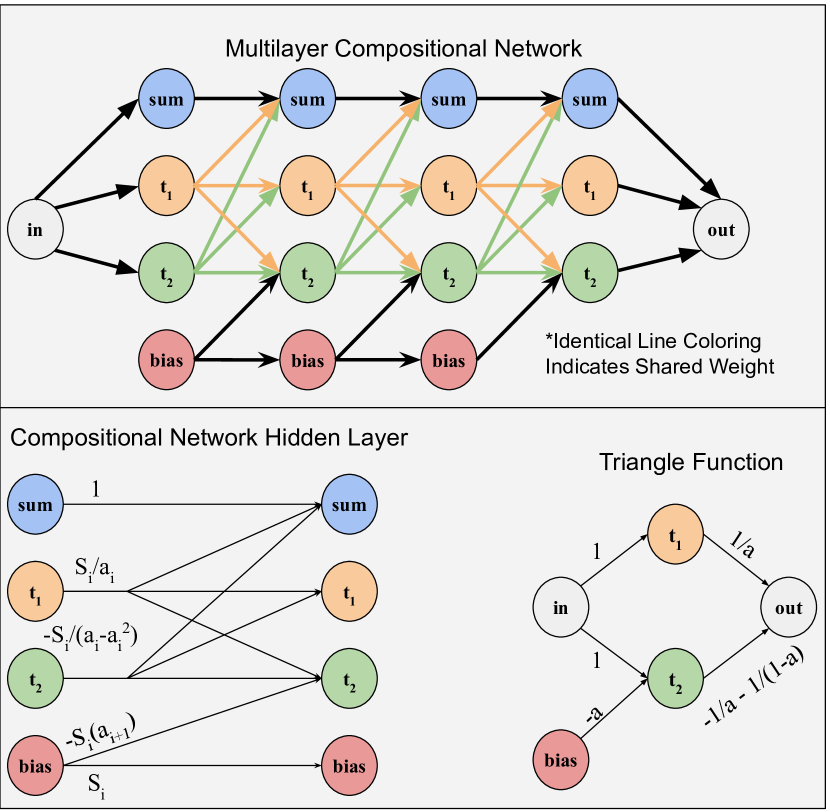
To encode these functions into a ReLU network, we begin with triangle functions. This is the subnetwork on the right in Figure 2. Its maximum output is at the peak location . Neuron simply preserves the input signal. Meanwhile, is negatively biased, deactivating it for inputs less than . Subtracting from changes the slope at the point where begins outputting a nonzero signal. The weight is picked to completely negate ’s positive influence, and then produce a negative slope. When these components are stacked the individual triangles they form will be composed, so it can be beneficial to think about each neuron in terms of its output waveform over the entire input domain . neurons are always active, so they hold complete triangle waves. neurons are deactivated for small inputs, so they hold an alternating sequence of triangles and inactive regions. This can be seen in Figure 3. Note how and use identical slopes where both are active.
Naively stacking the triangle generators from Figure 2 together would form a shape, but this is unnecessarily deep. We can replicate the one-dimensional function composition in the hidden layers on the left side of Figure 2 by using weight sharing instead. Any outgoing weight from or is shared; every neuron taking in a triangle wave does so by combining and in the same proportion. In this way, we can avoid having to use the extra intermediate neurons.
There are two other neurons in the compositional network’s layers. The accumulation neuron passes a weighted sum of all previous triangle waves through each layer. If this were naively implemented, it would multiply the and weights by the sum coefficients. Based on the derivations in Section 3.1, these coefficients will be exponentially decaying, so learning these weights directly may cause conditioning issues. Instead, the ratios between the coefficients are distributed amongst all the weights, so that the outputs of and neurons decay in amplitude in each layer. A conventional bias will have no connections to prior layers, so it will be unable to adjust to the weight decay. Therefore, a fourth neuron is configured to output a constant signal. Other neurons can then use their connection to it as a bias. This neuron will then connect to itself so that it can scale down with each layer.
3.1 Differentiability of Model Output
Because the reparameterization makes use of exponentially many linear regions, the functions it produces will have high complexity and be in danger of overfitting. To mitigate this we focus on constraining the network to have a differentiable output. While this is technically impossible for a finite network since the output will be piecewise linear; it is possible for a derivative to exist in the limit of infinite depth. We show that there is a unique choice of scaling parameters that is determined by the peaks of the composed triangle functions which can accomplish this. Enforcing a smooth solution during pretraining imparts a bias towards smoothness during the second training stage that will help the model avoid overfit solutions. The condition we derive is necessary for the existence of a derivative. In the appendix we show that it is also sufficient.
Recalling the earlier definition of the network output , we would like to select the based on in a manner where the derivative is defined on all of , which can only be done if the left and right hand derivative limits and agree.
Notationally, we will denote the sorted -locations of the peaks and valleys of by the lists and . We will use the list to reference the locations of all non-differentiable points, which we refer to as bends. . will denote finite depth approximations up to but not including layer . The error function will represent the error between the finite approximation and the infinite depth network.
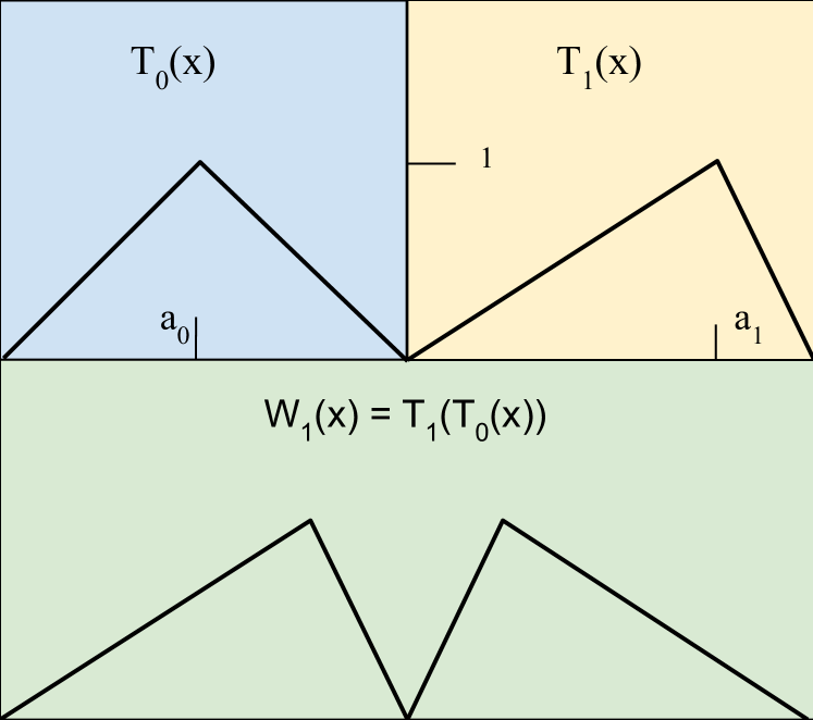
Figure 4 highlights some important properties about composing triangle functions. Peaks alternate with valleys. Peak locations in one layer become valleys in the next, and valleys persist. To produce , each line segment of becomes a dilated copy of . On negative slopes, the input to layer is reversed, so those copies are reflected. Each triangle function has two distinct slopes and which are dilated by the chain rule during the composition. Because the triangles are situated back to back, the slopes of on each side of a valley are proportional. New valleys are scaled by , while old ones are scaled by .
Before we begin reasoning about we note that it can simplify the analysis to only consider the derivative of the error function .
Lemma 3.1.
for , is continuous iff is continuous.
Proof.
All of for are differentiable at since will lie in the interior of a linear region of . Therefore, is continuous. Since , their difference is a continuous function, is continuous iff is continuous. ∎
Here we compute the right derivative of the error function. The left derivative will only be different by a constant factor.
Lemma 3.2.
For all , and are proportional to
| (4) |
Proof.
Let be some point in , and let be its index in any list it appears in. To calculate the value of , we will have to find the slope of the linear intervals to the immediate right of for all . The terms in the summation (4) mostly derive from the chain rule. We will use to represent . The first term in the sum will be . since the derivatives of composed functions will multiply. There are two different possible slope values of to multiply by, and the correct one to multiply is because is a peak of , so for . This gives . Note that the second term has the opposite sign as the first.
For all remaining terms, since was in , it is in for . For , and the chain rule applies the first slope . Since this slope is positive, every term has the opposite sign as the first. Summing up all the terms with the coefficients , and factoring out will yield the desired formula. Note that this same reasoning applies to the left side, the initial slope will just be different. ∎
Lemma 3.3.
If exists, it must be equal to 0.
Proof.
Let represent Equation (4), and and be the constants of proportionality for the directional derivatives. If , then for all . Since is comprised of alternating positive and negatively sloped line segments, and have opposite signs. The only way to satisfy the equation then is if . Consequently, for all . ∎
We can now prove our main theorem. Intuitively, the theorem shows that there is a way to sum the triangular waveforms so that the resulting function approximation converges to a differentiable function, which, as mentioned at the start of this subsection, can aid in preventing overfitting when using exponentially many linear regions. The idea of the proof is that much of the formula for will be shared between two successive generations of peaks. Once they are both valleys, they will behave the same, so the sizes of their remaining discontinuities will need to be proportional.
Theorem 3.4.
is continuous only if the scaling coefficients are selected based on according to:
| (5) |
Proof.
Rewriting Equation (4) (which is equal to 0) for layers and in the following way:
allows for a substitution to eliminate the infinite sum
Collecting all the terms gives
which simplifies to the desired result. ∎
4 Experiments
In this section, we implement our method to learn several convex one-dimensional curves. We present several important comparisons. To demonstrate how our networks make better use of depth, we benchmark against PyTorch’s default settings (nn.linear() uses Kaiming initialization), as well as the RAAI distribution from Singh & Sreejith (2021), and produce errors that are orders of magnitude lower than both. Additionally, we fix a set of initialization points such that the output is differentiable in the limit, and so that the output produces linear segments exponentially with depth. From these identical initialization points, we compare the effect of pretraining versus gradient descent alone. Lastly, we experiment with training the scaling parameters freely during pretraining, instead of choosing them to achieve differentiability. As in related papers (Perekrestenko et al., 2018; Daubechies et al., 2022), we restrict our attention to one-dimensional examples, which are sufficient to demonstrate our proposed theory and methodology.
4.1 Experimental Setup
All models are trained using Adam (Kingma & Ba, 2017) as the optimizer for 1000 epochs to ensure convergence. The data are 500 evenly spaced points on the interval for each of the curves. Each network is four neurons wide with five hidden layers, along with a one-dimensional input and output. The loss function used is the mean squared error, and the average and minimum loss are recorded for 30 models of each type. The networks unique to this paper share a common set of starting locations, so that the effects of each training regimen are directly comparable. The four curves we approximate are , , , and a quarter period of a sine wave. The curves are chosen to capture a variety of convex one dimensional functions. To approximate the sine and the hyperbolic tangent, the triangle waves are added to the line . For the other approximations, the waves are subtracted. This requires the first scaling factor to be instead of . These curves are simple, and the data is noiseless and synthetic, so we do not use a train-test split for these experiments. We instead focus on learning an interpolation of the data with a low MSE to show that effective representations can be found for these functions.
4.2 Numerical Results
| Network | Min | Min | Mean | Mean |
|---|---|---|---|---|
| Default Network | ||||
| RAAI Distribution | ||||
| No Pretraining | ||||
| Differentiability Not Enforced | ||||
| Differentiability Enforced |
| Network | Min | Min | Mean | Mean |
|---|---|---|---|---|
| Default Network | ||||
| RAAI Distribution | ||||
| No Pretraining | ||||
| Differentiability Not Enforced | ||||
| Differentiability Enforced |
Our main results are shown in Tables 1 and 2, wherein we observe several important trends. First, the worst performing networks are those that rely on purely randomized initializations. Even the networks that forgo pretraining benefit from initializing with many activation regions. When pretraining constraints are used, they are able to steer gradient descent to the best solutions, resulting in reductions in minimum error of three orders of magnitude over default networks.
Pretraining with differentiability enforced also closes the gap between the minimum and mean errors compared to other setups. This indicates that these loss landscapes are indeed the most reliable to traverse. When the scaling factors are trained separately, it can cause networks to exhibit behavior akin to overfitting. Even in our noiseless setting, we find that it is still possible to settle into local minima where the function interpolates only a small subset of the data points and fails to accurately represent the target curve in between them. Enforcing differentiability during pretraining can impart a bias towards smoother solutions during gradient descent and eliminates these occurrences in our experiments.
The last trend to observe is the poor average performance of default networks. In a typical run of these experiments, around half of the default networks collapse. RAAI is able to eliminate most, but not all of the dying ReLU instances due to its probabilistic nature, so it, too, has high mean error.
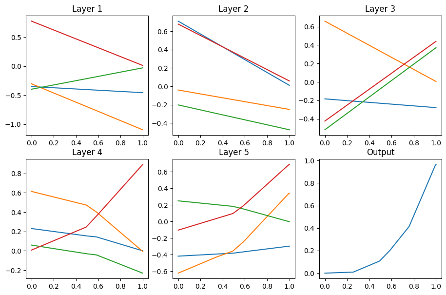
4.3 Gradient Descent does not Directly Optimize Efficiency
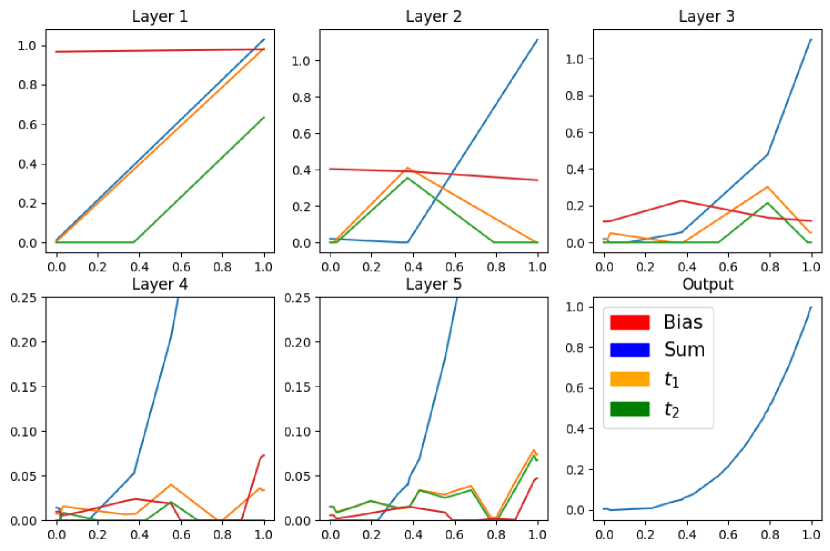
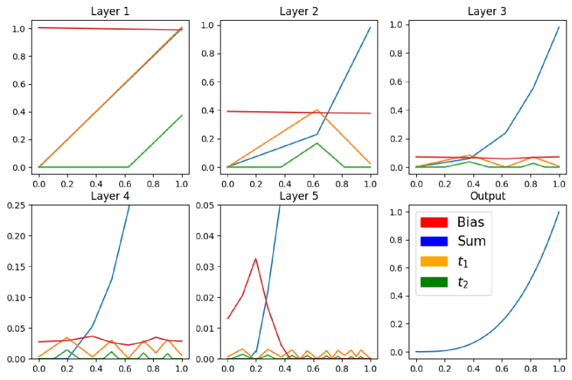
Figure 5 shows the interior of a default network. The layers here are shown before applying ReLU. The default networks fail to make efficient use of ReLU to produce linear regions, even falling short of 1 bend per neuron, which can easily be attained by forming a linear spline (1 hidden layer) that interpolates some of the data points. Rather than an exponential efficiency boost, depth is actually hindering these networks. Examining the figure, the first two layers are wasted. No neuron’s activation pattern crosses , so ReLU is never used. Layer 3 could be formed directly from the input signal. Deeper in the network, more neurons remain either strictly positive or negative. Those that intersect are monotonic, only able to introduce one bend at a time. The core issue is that while more bends leads to better accuracy, networks that have few bends are not locally connected in parameter space to those that have many. This is problematic since gradients can only carry information about the effects of infinitesimal parameter modifications. If a bend exists, gradient descent can reposition it. But for a neuron that always outputs a strictly positive value (such as the red in layer 2), bends cannot be introduced by infinitesimal weight or bias adjustments. Therefore, bend-related information will be absent from its gradients. Gradient descent will only introduce a network to bend by happenstance; indirectly related local factors must guide a neuron to begin outputting negative values. Rarely, these local incentives are totally absent, and the network outputs a bend-free line of best fit.
4.4 Inside the Compositional Networks
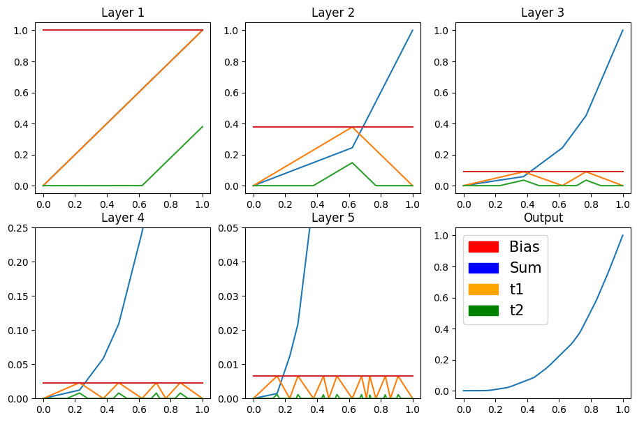
In Figure 6 we compare the top performing models with and without reparameterized pretraining. We observe that without the guidance of the pretraining, gradient descent usually loses the triangle generating structure. It typically happens around layer 4 or 5, devolving into noisy patterns and resulting in higher errors whereas pretraining maintains structure at greater depths. This behavior of gradient descent we observe is problematic since theoretical works often rely on specific constructions within networks to prove their results. Gradient descent greedily abandons any such structure in favor of models that can be worse in the long term. A theoretical result that shows a certain representation exists in the set of neural networks will thus have a hard time actually learning it without a subsequent plan to control training.
5 Limitations and Extensions
Although our reparemeterization can help maintain the triangular structure out to greater depths than unassisted gradient, our networks still lose structure eventually. This suggests that our reparameterization is limited in the functions it can represent. It may be enabling a rapid error reduction initially in the first few layers, but be unable to approach most curves to arbitrary precision. It is in this remaining error gap that the second stage gradient descent becomes lost. In the appendix, we detail two important results concerning the theoretical expressive power of our reparameterization that support this.
First, the differentiability constraints on the scaling parameters during pretraining necessitate that the network outputs a convex function. It is important for the pretraining to be able to produce a reasonably close initial solution; therefore, the reparameterization we use is only suitable for approximating convex functions. The second limitation we encounter is that pursuing further smoothness (at least in this 4-neuron configuration) is not possible. We show that approximating is the only way to have a twice continuously differentiable output in the infinite depth limit.
Despite these limitations, these networks could still be considered as replacements of the gate discussed in Section 2.1. Likewise, they could be used as a base component for assembly into larger networks. These composed networks could learn non-convex functions in higher dimensions, and they would at minimum be guaranteed to represent interpolating polynomials. The drawback is that they would likely become prohibitively large. Rather than approximating another approximation scheme out of ReLU networks, it may be better to focus on finding representations that more naturally arise from ReLU networks themselves when extending this work. Two properties specifically stand out as being somewhat fundamental to deep ReLU approximations: each linear region produced is a full copy of the original input interval , and the linear regions boundaries become dense as depth tends towards infinity. Density ensures that no two inputs are linearly related in an infinite network, and the repeated reproduction of the input space allows each layer to act on each previously existing region independently and simultaneously. These properties both arise in our method, and are likely important considerations when seeking theoretical extensions. Lastly, it might be important to consider non-differentiable model outputs as a way to gain additional flexibility, but additional protections would need to be put in place against overfitting.
6 Concluding Remarks
This paper focused on exploiting the potential computational complexity advantages neural networks offer for the problem of training efficient nonlinear function representations; in particular, compelling ReLU networks to approximate functions with exponential accuracy as network depth is linearly increased. Our results showed improvements of one to several orders of magnitude in using our reparameterization and pretraining strategy to train ReLU networks to learn various nonlinear, convex, one-dimensional functions. Though further research is required to extend this technique to general multi-dimensional nonlinear functions, the present work’s principal significance lies in demonstrating the possibility of converting theoretical ReLU-based constructions into novel training procedures. This finding is particularly powerful since random initialization and gradient descent are not likely to produce an efficient solution on their own, even if it can be proven to exist in the set of sufficiently sized ReLU networks. We are hopeful that future works by our group and others will help illuminate a complete theory for harnessing the potential exponential power of depth in ReLU networks and even more general types of neural networks.
Potential Broader Impact
This paper presents work whose goal is to enable more efficient neural networks. While the present work is largely theoretical, future advances in this line of research could enable the use of much smaller networks in many practical applications, which could substantially mitigate the rapidly growing issue of energy usage in large learning systems.
References
- Chen et al. (2019) Chen, M., Jiang, H., Liao, W., and Zhao, T. Efficient approximation of deep ReLU networks for functions on low dimensional manifolds. In Wallach, H., Larochelle, H., Beygelzimer, A., d'Alché-Buc, F., Fox, E., and Garnett, R. (eds.), Advances in Neural Information Processing Systems, volume 32. Curran Associates, Inc., 2019. URL https://proceedings.neurips.cc/paper_files/paper/2019/file/fd95ec8df5dbeea25aa8e6c808bad583-Paper.pdf.
- Chmielewski-Anders (2020) Chmielewski-Anders, A. Activation regions as a proxy for understanding neural networks. Master’s thesis, KTH Royal Institute of Technology, July 2020.
- Cybenko (1989) Cybenko, G. Approximation by superpositions of a sigmoidal function. Mathematics of control, signals and systems, 2(4):303–314, 1989.
- Daubechies et al. (2022) Daubechies, I., DeVore, R., Foucart, S., Hanin, B., and Petrova, G. Nonlinear approximation and (deep) ReLU networks. Constructive Approximation, 55(1):127–172, Feb 2022. ISSN 1432-0940. doi: 10.1007/s00365-021-09548-z. URL https://doi.org/10.1007/s00365-021-09548-z.
- Frankle & Carbin (2019) Frankle, J. and Carbin, M. The lottery ticket hypothesis: Finding sparse, trainable neural networks, 2019.
- Gibou et al. (2019) Gibou, F., Hyde, D., and Fedkiw, R. Sharp interface approaches and deep learning techniques for multiphase flows. Journal of Computational Physics, 380:442–463, 2019. doi: 10.1016/j.jcp.2018.05.031. URL https://doi.org/10.1016/j.jcp.2018.05.031.
- Glorot & Bengio (2010) Glorot, X. and Bengio, Y. Understanding the difficulty of training deep feedforward neural networks. In Teh, Y. W. and Titterington, M. (eds.), Proceedings of the Thirteenth International Conference on Artificial Intelligence and Statistics, volume 9 of Proceedings of Machine Learning Research, pp. 249–256, Chia Laguna Resort, Sardinia, Italy, 13–15 May 2010. PMLR. URL https://proceedings.mlr.press/v9/glorot10a.html.
- Hanin (2019) Hanin, B. Universal function approximation by deep neural nets with bounded width and ReLU activations. Mathematics, 7(10), 2019. ISSN 2227-7390. doi: 10.3390/math7100992. URL https://www.mdpi.com/2227-7390/7/10/992.
- Hanin & Rolnick (2019) Hanin, B. and Rolnick, D. Deep ReLU networks have surprisingly few activation patterns. In Wallach, H., Larochelle, H., Beygelzimer, A., d'Alché-Buc, F., Fox, E., and Garnett, R. (eds.), Advances in Neural Information Processing Systems, volume 32. Curran Associates, Inc., 2019. URL https://proceedings.neurips.cc/paper_files/paper/2019/file/9766527f2b5d3e95d4a733fcfb77bd7e-Paper.pdf.
- He et al. (2015) He, K., Zhang, X., Ren, S., and Sun, J. Delving deep into rectifiers: Surpassing human-level performance on imagenet classification. In Proceedings of the IEEE International Conference on Computer Vision (ICCV), December 2015.
- Hornik et al. (1989) Hornik, K., Stinchcombe, M., and White, H. Multilayer feedforward networks are universal approximators. Neural Networks, 2(5):359–366, 1989. ISSN 0893-6080. doi: https://doi.org/10.1016/0893-6080(89)90020-8. URL https://www.sciencedirect.com/science/article/pii/0893608089900208.
- Ivanova & Kubat (1995) Ivanova, I. and Kubat, M. Initialization of neural networks by means of decision trees. Knowledge-Based Systems, 8(6):333–344, 1995.
- Kingma & Ba (2017) Kingma, D. P. and Ba, J. Adam: A method for stochastic optimization, 2017.
- Liang & Srikant (2016) Liang, S. and Srikant, R. Why deep neural networks? CoRR, abs/1610.04161, 2016. URL http://arxiv.org/abs/1610.04161.
- Lu et al. (2021) Lu, J., Shen, Z., Yang, H., and Zhang, S. Deep network approximation for smooth functions. SIAM Journal on Mathematical Analysis, 53(5):5465–5506, jan 2021. doi: 10.1137/20m134695x. URL https://doi.org/10.1137/20m134695x.
- Lu et al. (2020) Lu, L., Shin, Y., Su, Y., and Karniadakis, G. E. Dying ReLU and initialization: Theory and numerical examples. Communications in Computational Physics, 28(5):1671–1706, 2020. ISSN 1991-7120. doi: https://doi.org/10.4208/cicp.OA-2020-0165. URL http://global-sci.org/intro/article_detail/cicp/18393.html.
- Lu et al. (2017) Lu, Z., Pu, H., Wang, F., Hu, Z., and Wang, L. The expressive power of neural networks: A view from the width. In Guyon, I., Luxburg, U. V., Bengio, S., Wallach, H., Fergus, R., Vishwanathan, S., and Garnett, R. (eds.), Advances in Neural Information Processing Systems, volume 30. Curran Associates, Inc., 2017. URL https://proceedings.neurips.cc/paper_files/paper/2017/file/32cbf687880eb1674a07bf717761dd3a-Paper.pdf.
- Montanelli et al. (2020) Montanelli, H., Yang, H., and Du, Q. Deep ReLU networks overcome the curse of dimensionality for bandlimited functions, 2020.
- Nag et al. (2023) Nag, S., Bhattacharyya, M., Mukherjee, A., and Kundu, R. Serf: Towards better training of deep neural networks using log-softplus error activation function. In Proceedings of the IEEE/CVF Winter Conference on Applications of Computer Vision (WACV), pp. 5324–5333, January 2023.
- Perekrestenko et al. (2018) Perekrestenko, D., Grohs, P., Elbrächter, D., and Bölcskei, H. The universal approximation power of finite-width deep relu networks, 2018.
- Qi et al. (2024) Qi, X., Wei, Y., Mei, X., Chellali, R., and Yang, S. Comparative analysis of the linear regions in ReLU and LeakyReLU networks. In Luo, B., Cheng, L., Wu, Z.-G., Li, H., and Li, C. (eds.), Neural Information Processing, pp. 528–539, Singapore, 2024. Springer Nature Singapore. ISBN 978-981-99-8132-8.
- Shin & Karniadakis (2020) Shin, Y. and Karniadakis, G. E. Trainability of ReLU networks and data-dependent initialization. Journal of Machine Learning for Modeling and Computing, 1(1):39–74, 2020. ISSN 2689-3967.
- Singh & Sreejith (2021) Singh, D. and Sreejith, G. J. Initializing ReLU networks in an expressive subspace of weights, 2021.
- Telgarsky (2015) Telgarsky, M. Representation benefits of deep feedforward networks, 2015.
- Wang et al. (2018) Wang, Q. et al. Exponential convergence of the deep neural network approximation for analytic functions. arXiv preprint arXiv:1807.00297, 2018.
- Yarotsky (2017) Yarotsky, D. Error bounds for approximations with deep ReLU networks. Neural Networks, 94:103–114, 2017. ISSN 0893-6080. doi: https://doi.org/10.1016/j.neunet.2017.07.002. URL https://www.sciencedirect.com/science/article/pii/S0893608017301545.
Appendix A Appendix
A.1 Sufficiency for differentiability
We can show that in addition to being necessary for continuity of the derivative, our choice of scaling is sufficient when are bounded away from 0 or 1.
Theorem A.1.
is continuous if we can find such that for all .
Proof.
We begin by considering Equation (4) for layer .
Recall that this equation is telling us about the size of the discontinuities in the derivative as triangle waves are added. Each time a triangle wave is added, it can be thought of as subtracting the terms on the right. We will prove our result by substituting Equation (5) into this formula, and then verifying that the resulting equation is valid. First we would like to rewrite each in terms of . Equation (5) gives a recurrence relation. Converting it to an explicit representation we have:
| (6) |
When we substitute this into Equation (4), three things happen: each term is divisible by so cancels out, every factor in the product except the last cancels, and cancels. This leaves
| (7) |
We will now argue that each term of the sum on the right accounts for a fraction (equal to ) of the remaining error. Inductively we can show:
| (8) |
Intuitively, this means as long as the first term appearing on the right is repeatedly subtracted, that term is always equal to times the left side. As a base case, we have . Assuming the above equation holds for all previous values of
using the inductive hypothesis to make the substitution
Since all , the size of the discontinuity at the points is upper bounded and lower bounded by exponentially decaying series. Since both series approach zero, so does the series here. ∎
This lemma shows that the derivative of the finite approximation excluding is the same as that of the infinite sum.
Lemma A.2.
For all :
| (9) |
Proof.
From the previous lemma we know . . The sum of the first terms are differentiable at the points since they lie between the discontinuities at . ∎
A.2 Second Derivatives
Here we show that any function represented by one of these networks that is not does not have a continuous second derivative. To show this we will sample a discrete series of values from and show that the left and right hand limits are not equal (unless ), which will imply that the continuous version of the limit for the second derivative does not exist. First we will produce the series of . Let be the location of a peak at layer , and let and be its immediate neighbors in .
Lemma A.3.
If for all , we have . Furthermore, for any finite .
Proof.
Let be a constant of proportionality for the slopes on the left and right of in layer . These slopes are proportional to and depending on which way the triangle encompassing is oriented ( could have been positive or negative at its location), We will denote these as and and reason about them later. is a peak location of , so on the left side slope is negative and the right is positive. Solving for the location of on each side will give and .
On each subsequent iteration , is a valley point and the intervals get multiplied by . is a valley point so the left slope is positive and the right is negative, and , are peak points. The slope magnitudes are given by and since oscillates from 0 to 1 over these spans. Solving for the new peaks again will give and . The resulting non-recursive formulas are:
| (10) |
The right hand sides will never be equal to zero with a finite number of terms since parameters are bounded away from and by . ∎
Next we derive the values of to complete the proof.
Theorem A.4.
A compositional network with a second differentiable output necessarily outputs .
Proof.
The points and are all peak locations, (9) gives their derivative values as . Earlier we reasoned about the sizes of the discontinuities in at , since and always lie on the linear intervals surrounding as , we can get the value of using (8) with the initial discontinuity size set to rather than 1. Focusing on the right hand side we get:
taking gives a series:
The issue which arises is that the derivation on the left is identical, except for a replacement of by . The only way for these formulas to agree then is for which implies . ∎
A.3 Error Decay
Lastly, we show that the error of these approximations decays exponentially.
Lemma A.5.
The ratio is at most .
Proof.
by applying formula (5) twice, we have
To maximize we choose and . The quantity is a parabola with a maximum of at . ∎
Lemma A.6.
The function is convex.
Proof.
To establish this we will introduce the list , which tracks the values of the derivative at the th set of valley points. All but the first and last points will have been peaks at some point in their history, so Equation (9) gives the value of those derivatives as .
We establish an inductive invariant that the y-values in the list remain sorted in descending order, and that for .
Before any of are added, is a line with derivative 0, is its two endpoints. is positive for the left endpoint (negative for right) since on the far edges is a sum of a series of positive (or negative) slopes, Therefore the points in are in descending sorted order. The second part of the invariant is true since 0 is in between those values.
Consider an arbitrary interval of , this entire interval is between two valley points, so (which hasn’t added yet) is some constant value in between and . The point will have , and it will become a member of . This means we will have , maintaining sorted order.
Adding takes to splitting each constant valued interval in two about the points , increasing the left side, and decreasing the right side. Recalling from the derivation of (4) all terms but the first in the sum have the same sign, so the values in are approached monotonically. Therefore on the left interval we have and on the right we have . And so remains monotone decreasing. ∎
Theorem A.7.
The approximation error decays exponentially.
Proof.
To get this result, we apply the previous two lemmas. Since is convex, it lies above any line segment connecting any two points on the curve. for all , but for points in . Since the bend points are only of nonzero value once, for all points in . is made of line segments and equals repeatedly, will be a series of positively valued curve segments. The derivative will still be decreasing on each of these intervals since it was just shifted by a constant, and each of these intervals will be convex itself.
Since for , these points will be the locations of maximum error. Since they only have nonzero value in , and is convex, . Since decay exponentially, we have our result. ∎