Anomalies in Hadronic $B$ Decays

Abstract

In this paper, we perform fits to $B\to PP$ decays, where $B=\{B^{0},B^{+},B_{s}^{0}\}$ and the pseudoscalar $P=\{\pi,K\}$, under the assumption of flavor SU(3) symmetry [SU(3)_F]. Although the fits to $\Delta S=0$ or $\Delta S=1$ decays individually are good, the combined fit is very poor: there is a $3.6\sigma$ disagreement with the SM. One can remove this discrepancy by adding SU(3)_F-breaking effects, but 1000% SU(3)_F breaking is required. The above results are rigorous, group-theoretically – no dynamical assumptions have been made. When one adds an assumption motivated by QCD factorization, the discrepancy with the SM grows to $4.4\sigma$.

For the past 10$+$ years, there has been an enormous amount of interest in the semileptonic $B$ anomalies involving the decays $b\to s\ell^{+}\ell^{-}$ ($\ell=\mu,e$) and $b\to c\tau^{-}{\bar{\nu}}_{\tau}$. Interestingly, there have also been hadronic $B$ anomalies, but these have generally flown under the radar. The $B\to\pi K$ puzzle has been around for about 20 years (see Refs. [1, 2] and references therein), but discrepancies in other sets of hadronic decays have recently been pointed out. These include the U-spin puzzle [3], three puzzles involving $B_{s}^{0}\to K^{0}\overline{K}^{0}$ [4], and a puzzle in $B_{d,s}^{0}\to K^{(*)0}\overline{K}^{(*)0}$ decay [5]. Of these four, the first three involve only $B\to PP$ decays, where $B=\{B^{0},B^{+},B_{s}^{0}\}$, and the pseudoscalar $P=\{\pi,K\}$. This class of $B$ decays is the focus of our study.

In all of these puzzles, one has a set of $B$ decays whose amplitudes are related, either by a symmetry, or simply by having the same quark-level decay. The $B\to\pi K$ puzzle involves the four decays $B^{+}\to\pi^{0}K^{+}$, $B^{+}\to\pi^{+}K^{0}$, $B^{0}\to\pi^{-}K^{+}$, and $B^{0}\to\pi^{0}K^{0}$, whose amplitudes form an isospin quadrilateral. U spin relates the decays $B_{d,s}^{0}\to P^{\pm}P^{\prime\mp}$, where $P$ and $P^{\prime}$ are each $\pi$ or $K$. And $B_{s}^{0}\to K^{0}\overline{K}^{0}$ is related to $B_{s}^{0}\to K^{+}K^{-}$ by isospin, to $B^{0}\to K^{0}\overline{K}^{0}$ by U spin, and to $B^{+}\to\pi^{+}K^{0}$ by virtue of having the same quark-level decay. In each set of related decays, the puzzle arises because it is found that the measured values of the observables of all the related decays are not consistent with one another.

The key point here is that all of these $B\to PP$ decays are related to one another by flavor SU(3) symmetry [SU(3)_F]. By performing a global fit to all the $B\to PP$ observables under the assumption of SU(3)_F, these puzzles can be combined, and one can quantify just how well (or poorly) the standard model (SM) explains the data. Analyses of this type were done many years ago [6], using diagrams as the theoretical parameters and making dynamical assumptions in order to neglect certain diagrams. But today there is enough data that no approximations are necessary – a full SU(3)_F fit can be performed. There are even enough observables in the fit to quantify a number of SU(3)_F-breaking effects. As we will see, there are serious discrepancies with the SM.

We are interested in charmless $B\to PP$ decays, which are associated with the transitions ${\bar{b}}\to{\bar{u}}u{\bar{q}}$ and ${\bar{b}}\to{\bar{q}}$, $q=d,s$. The weak Hamiltonian is [7]

$$H_{W} = \frac{G_{F}}{\sqrt{2}}\sum_{q=d,s}\left(\lambda_{u}^{(q)}\left[c_{1}({\bar{b}}u)_{V-A}({\bar{u}}q)_{V-A}\right.\right.$$ (1)

$$\left.\left.+~{}c_{2}({\bar{b}}q)_{V-A}({\bar{u}}u)_{V-A}\right]-\lambda_{t}^{(q)}\sum_{i=3}^{7}c_{i}Q_{i}^{(q)}\right)~{},$$

where $\lambda_{q^{\prime}}^{(q)}=V_{q^{\prime}b}^{*}V_{q^{\prime}q}$, $q=d,s$, $q^{\prime}=u,c,t$. Here the $c_{i}$ ($i=1$-10) are Wilson coefficients, and $Q_{i}^{(q)}$ represent penguin operators of two kinds: gluonic ($i=3$-6) and electroweak ($i=7$-10). $H_{W}$ transforms as a ${\bf 3^{*}_{1}}$, ${\bf 3^{*}_{2}}$, ${\bf 6}$, or ${\bf 15^{*}}$ of SU(3)_F. The initial $B$ is a ${\bf 3}$ and the final state is $({\bf 8}\times{\bf 8})_{s}={\bf 1}+{\bf 8}+{\bf 27}$. Putting these all together, charmless $B\to PP$ decays are described by seven reduced matrix elements (RMEs). These are:

$$\lambda_{u}^{(q)} : A_{1}=\langle{\bf 1}||{\bf 3^{*}_{1}}||{\bf 3}\rangle~{},~{}A_{8}=\langle{\bf 8}||{\bf 3^{*}_{1}}||{\bf 3}\rangle~{},~{}$$

$$\lambda_{t}^{(q)} : B_{1}=\langle{\bf 1}||{\bf 3^{*}_{2}}||{\bf 3}\rangle~{},~{}B_{8}=\langle{\bf 8}||{\bf 3^{*}_{2}}||{\bf 3}\rangle~{},$$

$$\lambda_{u}^{(q)}~{}{\&}~{}\lambda_{t}^{(q)} : R_{8}=\langle{\bf 8}||{\bf 6}||{\bf 3}\rangle~{},~{}P_{8}=\langle{\bf 8}||{\bf 15^{*}}||{\bf 3}\rangle~{},~{}$$ (2)

$$~{}~{}~{}~{}~{}~{}~{}~{}P_{27}=\langle{\bf 27}||{\bf 15^{*}}||{\bf 3}\rangle~{}.~{}~{}$$

If SU(3)_F is unbroken, these RMEs are the same for $\Delta S=0$ and $\Delta S=1$ decays. However, they can be different if SU(3)_F-breaking effects are allowed.

The idea is then to express the amplitudes for all charmless $B\to PP$ decays in terms of these seven RMEs, and then to perform a fit. However, before doing this, we note that an equivalent description of these SU(3)_F amplitudes is provided by quark diagrams [8, 9]. There are eight topologies, representing tree ($T$), color-suppressed tree ($C$), annihilation ($A$), $W$-exchange ($E$), penguin ($P$), penguin-annihilation ($PA$), electroweak penguin ($P_{EW}$) and color-suppressed electroweak penguin ($P^{C}_{EW}$) amplitudes. $T$, $C$, $E$ and $A$ are associated with $\lambda_{u}^{(q)}$, while $P_{EW}$ and $P^{C}_{EW}$ are associated with $\lambda_{t}^{(q)}$. $P$ and $PA$ each have three pieces, related to the flavor of the up-type quark in the loop. When CKM unitarity is imposed to remove the $c$-quark pieces, $P_{uc}$ and $PA_{uc}$ are associated with $\lambda_{u}^{(q)}$, $P_{tc}$ and $PA_{tc}$ with $\lambda_{t}^{(q)}$. Previously, it was often customary to absorb magnitudes of CKM matrix elements into these diagrams. However, in this paper the CKM factors are kept separate.

In order to find how RMEs are related to diagrams, one has to compare the expressions for amplitudes in terms of diagrams with those in terms of RMEs [10]. The five RMEs associated with $\lambda_{u}^{(q)}$ are related to the six diagrams $T$, $C$ $A$, $E$, $P_{uc}$ and $PA_{uc}$ (e.g., see Ref. [8]). These diagrams only appear in five combinations, and it is convenient to eliminate $E$ by defining five effective diagrams:

$${\widetilde{T}}\equiv T+E~{},~{}~{}{\widetilde{C}}\equiv C-E~{},~{}~{}{\widetilde{A}}\equiv A+E~{},$$

$$\hskip 17.07164pt{\widetilde{P}}_{uc}\equiv P_{uc}-E~{},~{}~{}{\widetilde{PA}}_{uc}\equiv PA_{uc}+E~{}.$$ (3)

The relations between the RMEs and these effective diagrams are as follows :

$$A_{1} = \frac{1}{2\sqrt{3}}\left(-3{\widetilde{T}}+{\widetilde{C}}-8{\widetilde{P}}_{uc}-12{\widetilde{PA}}_{uc}\right)~{},$$

$$A_{8} = \frac{1}{8}\sqrt{\frac{5}{3}}\left(-3{\widetilde{T}}+{\widetilde{C}}-8{\widetilde{P}}_{uc}-3{\widetilde{A}}\right)~{},$$

$$R_{8} = \frac{\sqrt{5}}{4}\left({\widetilde{T}}-{\widetilde{C}}-{\widetilde{A}}\right)~{},$$

$$P_{8} = \frac{1}{8\sqrt{3}}\left({\widetilde{T}}+{\widetilde{C}}+5{\widetilde{A}}\right)~{},$$

$$P_{27} = -\frac{1}{2\sqrt{3}}\left({\widetilde{T}}+{\widetilde{C}}\right)~{}.$$ (4)

The relations between diagrams and the two RMEs associated with $\lambda_{t}^{(q)}$ are

$$B_{1}=-\frac{4}{\sqrt{3}}\left(\frac{3}{2}PA_{tc}+P_{tc}\right)~{},~{}~{}B_{8}=-\sqrt{\frac{5}{3}}P_{tc}~{}.$$ (5)

Finally, the electroweak penguin diagrams $P_{EW}$ and $P^{C}_{EW}$ are also related to RMEs. But since there are only seven RMEs, and since all of these are related to other diagrams (see above), $P_{EW}$ and $P^{C}_{EW}$ must be related to these other diagrams. These relations are [12, 13, 14]

$$P^{(C)}_{EW}=\frac{3}{4}\left[\frac{\Sigma_{9}}{\Sigma_{1}}({\widetilde{T}}+{\widetilde{C}}+{\widetilde{A}})\mathbin{\vbox{\hbox{\oalign{\hfil$\scriptstyle+$\hfil\cr\kern-1.29167pt\cr$\scriptscriptstyle({-})$\cr}}}}\frac{\Delta_{9}}{\Delta_{1}}({\widetilde{T}}-{\widetilde{C}}-{\widetilde{A}})\right]~{},$$ (6)

where $\Sigma_{1}=c_{1}+c_{2},\Delta_{1}=c_{1}-c_{2},\Sigma_{9}=c_{9}+c_{10},$ and $\Delta_{9}=c_{9}-c_{10}$. Here we have kept only the contributions from $Q_{9}$ and $Q_{10}$ of Eq. (1). This is justified because the Wilson coefficients of the two other electroweak penguin operators $Q_{7}$ and $Q_{8}$ are tiny [7].

This shows that diagrams are equivalent to RMEs. An analysis that uses diagrams to parametrize amplitudes is therefore completly rigorous from a group-theoretical point of view. One advantage of diagrams over RMEs is that it is straightforward to work out the contribution of any diagram to a given decay amplitude. It is not necessary to compute the SU(3)_F Clebsch-Gordan coefficients, which can be tricky.

Another advantage is that one can estimate the relative sizes of different diagrams. For example, it has been argued that $E$, $A$ and $PA$ are much smaller than the other diagrams because they involve an interaction with the spectator quark [8, 9], and so can (often) be neglected. But this is also problematic: results that use dynamical assumptions such as this are not rigorous group-theoretically. In addition, one has to worry about whether the assumptions remain valid when rescattering effects are included.

In this paper, we make no such assumptions. The amplitudes are parametrized in terms of all the diagrams, and we perform fits to the data [[Asimilaranalysis, inwhichtheunknownparametersaredefinedwithinQCDfactorization, canbefoundin~]Huber:2021cgk]. The sizes of the diagrams are fixed by the data. It is only at the end that we examine the effects of adding dynamical assumptions.

Decay	$\lambda^{(d)}_{u}$					$\lambda^{(d)}_{t}$
Mode	${\widetilde{T}}$	${\widetilde{C}}$	${\widetilde{P}}_{uc}$	${\widetilde{A}}$	${\widetilde{PA}}_{uc}$	${P}_{tc}$	${PA}_{tc}$	${P_{EW}}$	${P_{EW}^{C}}$
$B^{+}\to\overline{K}^{0}K^{+}$	0	0	1	1	0	1	0	0	$-\frac{1}{3}$
$B^{+}\to\pi^{0}\pi^{+}$	$-\frac{1}{\sqrt{2}}$	$-\frac{1}{\sqrt{2}}$	0	0	0	0	0	$-\frac{1}{\sqrt{2}}$	$-\frac{1}{\sqrt{2}}$
$B^{0}\to K^{0}\overline{K}^{0}$	0	0	1	0	1	1	1	0	$-\frac{1}{3}$
$B^{0}\to\pi^{+}\pi^{-}$	$-1$	0	-1	0	$-1$	$-1$	$-1$	0	$-\frac{2}{3}$
$B^{0}\to\pi^{0}\pi^{0}$	0	$-\frac{1}{\sqrt{2}}$	$\frac{1}{\sqrt{2}}$	0	$\frac{1}{\sqrt{2}}$	$\frac{1}{\sqrt{2}}$	$\frac{1}{\sqrt{2}}$	$-\frac{1}{\sqrt{2}}$	$-\frac{1}{3\sqrt{2}}$
$B^{0}\to K^{+}K^{-}$	0	0	0	0	$-1$	0	$-1$	0	0
$B_{s}^{0}\to\pi^{+}K^{-}$	$-1$	0	$-1$	0	0	$-1$	0	0	$-\frac{2}{3}$
$B_{s}^{0}\to\pi^{0}\overline{K}^{0}$	0	$-\frac{1}{\sqrt{2}}$	$\frac{1}{\sqrt{2}}$	0	0	$\frac{1}{\sqrt{2}}$	0	$-\frac{1}{\sqrt{2}}$	$-\frac{1}{3\sqrt{2}}$

Table 1: Decomposition of $\Delta S=0$ $B\to PP$ decay amplitudes in terms of diagrams.

There are eight $B\to PP$ decays with $\Delta S=0$ and eight with $\Delta S=1$. The decomposition of their amplitudes in terms of diagrams is given in Tables 1 and 2, respectively. Diagrams for $\Delta S=0$ and $\Delta S=1$ processes are respectively written without and with primes. Of course, in the limit of perfect SU(3)_F symmetry, ${\widetilde{T}}^{\prime}={\widetilde{T}}$, etc.

Decay	$\lambda^{(s)}_{u}$					$\lambda^{(s)}_{t}$
Mode	${\widetilde{T}}^{\prime}$	${\widetilde{C}}^{\prime}$	${\widetilde{P}}^{\prime}_{uc}$	${\widetilde{A}}^{\prime}$	${\widetilde{PA}}^{\prime}_{uc}$	$P^{\prime}_{tc}$	$PA^{\prime}_{tc}$	$P^{\prime}_{EW}$	${P_{EW}^{\prime C}}$
$B^{+}\to\pi^{+}K^{0}$	0	0	1	1	0	1	0	0	$-\frac{1}{3}$
$B^{+}\to\pi^{0}K^{+}$	$-\frac{1}{\sqrt{2}}$	$-\frac{1}{\sqrt{2}}$	$-\frac{1}{\sqrt{2}}$	$-\frac{1}{\sqrt{2}}$	0	$-\frac{1}{\sqrt{2}}$	0	$-\frac{1}{\sqrt{2}}$	$-\frac{\sqrt{2}}{3}$
$B^{0}\to\pi^{-}K^{+}$	$-1$	0	$-1$	0	0	$-1$	0	0	$-\frac{2}{3}$
$B^{0}\to\pi^{0}K^{0}$	0	$-\frac{1}{\sqrt{2}}$	$\frac{1}{\sqrt{2}}$	0	0	$\frac{1}{\sqrt{2}}$	0	$-\frac{1}{\sqrt{2}}$	$-\frac{1}{3\sqrt{2}}$
$B_{s}^{0}\to K^{+}K^{-}$	$-1$	0	$-1$	0	$-1$	$-1$	$-1$	0	$-\frac{2}{3}$
$B^{0}_{s}\to K^{0}\overline{K}^{0}$	0	0	1	0	1	1	1	0	$-\frac{1}{3}$
$B^{0}_{s}\to\pi^{+}\pi^{-}$	0	0	0	0	$-1$	0	$-1$	0	0
$B^{0}_{s}\to\pi^{0}\pi^{0}$	0	0	0	0	$\frac{1}{\sqrt{2}}$	0	$\frac{1}{\sqrt{2}}$	0	0

Table 2: Decomposition of $\Delta S=1$ $B\to PP$ decay amplitudes in terms of diagrams.

Of the 16 charmless $B\to PP$ decays, 15 have been observed. Their measurements have given rise to a large number of observables (CP-averaged branching ratios or ${\cal B}_{CP}$, direct CP asymmetries or $A_{CP}$, and indirect CP asymmetries or $S_{CP}$). A complete list of these observables, along with their present experimental values, can be found in Tables 3 and 4. In terms of the theoretical parameters, the observables are defined as

$${\cal B}_{CP}=\frac{\sqrt{m_{B}^{2}-(m_{P_{1}}+m_{P_{2}})^{2}}\sqrt{m_{B}^{2}-(m_{P_{1}}-m_{P_{2}})^{2}}(|A|^{2}+|{\bar{A}}|^{2})\,S}{32\pi\,m_{B}^{3}\,\Gamma_{B}}~{},$$

$$A_{CP}=\frac{|{\bar{A}}|^{2}-|A|^{2}}{|{\bar{A}}|^{2}+|A|^{2}}~{}~{},~{}~{}~{}~{}S_{CP}=2{\rm Im}\left(\frac{q}{p}\frac{{\bar{A}}A^{*}}{|{\bar{A}}|^{2}+|A|^{2}}\right)~{}.$$ (7)

Here $A$ and ${\bar{A}}$ are the amplitudes for $B\to PP$ and its CP-conjugate process, respectively, $S$ is a statistical factor related to identical particles in the final state, and $q/p=\exp(-2i\phi_{M})$, where $\phi_{M}$ is the weak phase of $B_{q}^{0}$-${\bar{B}}_{q}^{0}$ mixing. Note that, for the direct CP asymmetry, some experiments present the result for $C_{CP}=-A_{CP}$. In the Tables, we have added the appropriate minus signs, so that all results are for $A_{CP}$. Also, in the fits, $S_{CP}$ is multiplied by $\eta_{CP}$, the CP of the final state. In general $\eta_{CP}=1$. The only exception is the final state $\pi^{0}K_{S}$, for which $\eta_{CP}=-1$.

Decay	${\cal B}_{CP}$ ($\times 10^{-6}$)	$A_{CP}$	$S_{CP}$
$B^{+}\to K^{+}\overline{K}^{0}$	1.31$\pm$0.14	0.04$\pm$0.14†
$B^{+}\to\pi^{+}\pi^{0}$	5.59$\pm$0.31	0.008$\pm$0.035
$B^{0}\to K^{0}\overline{K}^{0}$	1.21$\pm$0.16†	0.06$\pm$0.26	$-1.08\pm$0.49
$B^{0}\to\pi^{+}\pi^{-}$	5.15$\pm$0.19	0.311$\pm$ 0.030	$-0.666\pm$ 0.029
$B^{0}\to\pi^{0}\pi^{0}$	1.55$\pm$ 0.16	0.30$\pm$0.20
$B^{0}\to K^{+}K^{-}$	0.080$\pm$0.015
$B^{0}_{s}\to\pi^{+}K^{-}$	$5.90^{+0.87}_{-0.76}$	0.225$\pm$0.012
$B^{0}_{s}\to\pi^{0}\overline{K}^{0}$

Table 3: Measured values ${\cal B}_{CP}$, $A_{CP}$, and $S_{CP}$ in $\Delta S=0$ $B\to PP$ decays. The ^† indicates data taken from the Particle Data Group [16]. All other data are taken from HFLAV [17].

Decay	${\cal B}_{CP}$ ($\times 10^{-6}$)	$A_{CP}$	$S_{CP}$
$B^{+}\to\pi^{+}K^{0}$	23.52$\pm$0.72	$-0.016\pm$0.015
$B^{+}\to\pi^{0}K^{+}$	13.20$\pm$0.46	0.029$\pm$0.012
$B^{0}\to\pi^{-}K^{+}$	19.46$\pm$0.46	$-0.0836\pm$0.0032
$B^{0}\to\pi^{0}K^{0}$	10.06$\pm$0.43	$-0.01\pm$0.10	$0.57\pm$0.17
$B^{0}_{s}\to K^{+}K^{-}$	$26.6^{+3.2}_{-2.7}$	$-0.17\pm$0.03	0.14$\pm$0.03
$B^{0}_{s}\to K^{0}\overline{K}^{0}$	17.4$\pm$3.1
$B^{0}_{s}\to\pi^{+}\pi^{-}$	$0.72^{+0.11}_{-0.10}$
$B^{0}_{s}\to\pi^{0}\pi^{0}$	2.8$\pm$2.8∗

Table 4: Measured values of ${\cal B}_{CP}$, $A_{CP}$, and $S_{CP}$ in $\Delta S=1$ $B\to PP$ decays. The ^∗ indicates data taken from Ref. [18]. All remaining data are taken from HFLAV [17].

Consider first $\Delta S=0$ decays. The amplitudes are a function of 7 diagrams, corresponding to 13 unknown theoretical parameters (7 magnitudes, 6 relative strong phases). From Table 3, we see that there are 15 measured observables. The amplitudes also depend on the weak phases $\gamma$, $\beta$ (in $B^{0}$-${\bar{B}}^{0}$ mixing) and $\phi_{s}$ (in $B_{s}^{0}$-${\bar{B}}_{s}^{0}$ mixing), as well as on the CKM matrix elements involved in $\lambda_{u,t}^{(q)}$. Values for all of these quantities, including errors, are taken from the Particle Data Group (PDG) [16].

As the quantities taken from the PDG are “known,” we therefore effectively have 15 equations in 13 unknowns, so we can do a fit. The fit is performed using the program MINUIT [19, *James:2004xla, *James:1994vla, *iminuit]. We find an excellent fit: the $\chi_{\rm min}^{2}/{\rm d.o.f.}=0.35/2$, for a $p$-value of 0.84. The SM therefore has no difficulty explaining the $\Delta S=0$ data.

Turning to $\Delta S=1$ decays, there are again 13 unknown theoretical parameters, along with 15 measured observables (Table 4), so a fit can be performed. Here the fit is slightly worse, but still perfectly acceptable: $\chi_{\rm min}^{2}/{\rm d.o.f.}=1.8/2$, for a $p$-value of 0.40.

If one assumes perfect SU(3)_F symmetry, the diagrams in $\Delta S=0$ and $\Delta S=1$ decays are the same. We can therefore perform a fit including all the data – we have 30 equations in 13 unknowns. But now a serious problem arises: the best fit has $\chi_{\rm min}^{2}/{\rm d.o.f.}=43.8/17$, for a $p$-value of $3.6\times 10^{-4}$. This means that the data disagrees with the SM at the level of $3.6\sigma$. This is the anomaly in hadronic $B$ decays.

We stress again that no dynamical assumptions have been made regarding the diagrams. This result is completely rigorous from a group-theoretical point of view.

But this raises an obvious question. We know that SU(3)_F is broken in the SM. What is usually quoted as evidence is the fact that $f_{K}/f_{\pi}-1=~{}\sim 20\%$. That is, we naively expect SU(3)_F-breaking effects at this level. If such effects were included, perhaps that would remove the discrepancy.

Fortunately, the fit contains enough information to address this question. Above, we found that, when one considers only $\Delta S=0$ or $\Delta S=1$ decays, the fits are good. In Table 5, for each fit we show the best-fit values of the magnitudes of the diagrams. In the SU(3)_F limit, the diagrams in $\Delta S=0$ decays ($D$) are the same as those in $\Delta S=1$ decays ($D^{\prime}$). Thus, the ratios $|D^{\prime}/D|$ provide an indication of the level of SU(3)_F breaking required for the SM to explain the data.

These ratios are also shown in Table 5. For the diagrams associated with $\lambda_{u}^{(q)}$, this ratio is $\sim 10$, which corresponds to 1000% SU(3)_F breaking! This is obviously much larger than the $\sim 20\%$ of $f_{K}/f_{\pi}$. Thus, if the SM really does explain the data, then either the $3.5\sigma$ discrepancy is simply a statistical fluctuation (involving several different decays), or the SM breaks flavor SU(3)_F symmetry at an unexpectedly large level.

	$|{\widetilde{T}}|$	$|{\widetilde{C}}|$	$|{\widetilde{P}}_{uc}|$	$|{\widetilde{A}}|$
Fit	$4.0\pm 0.5$	$6.6\pm 0.7$	$3\pm 4$	$6\pm 5$
$\Delta S=0$	$|{\widetilde{PA}}_{uc}|$	$|P_{tc}|$	$|PA_{tc}|$
	$0.7\pm 0.8$	$0.8\pm 0.4$	$0.2\pm 0.4$
	$|{\widetilde{T}}^{\prime}|$	$|{\widetilde{C}}^{\prime}|$	$|{\widetilde{P}}^{\prime}_{uc}|$	$|{\widetilde{A}}^{\prime}|$
Fit	$48\pm 14$	$41\pm 14$	$48\pm 15$	$81\pm 28$
$\Delta S=1$	$|{\widetilde{PA}}^{\prime}_{uc}|$	$|P^{\prime}_{tc}|$	$|PA^{\prime}_{tc}|$
	$7\pm 4$	$0.78\pm 0.16$	$0.24\pm 0.04$
	$|{\widetilde{T}}^{\prime}/{\widetilde{T}}|$	$|{\widetilde{C}}^{\prime}/{\widetilde{C}}|$	$|{\widetilde{P}}^{\prime}_{uc}/{\widetilde{P}}_{uc}|$	$|{\widetilde{A}}^{\prime}/{\widetilde{A}}|$
	$12\pm 4$	$6.6\pm 2.2$	$16\pm 22$	$14\pm 13$
	$|{\widetilde{PA}}^{\prime}_{uc}/{\widetilde{PA}}_{uc}|$	$|P^{\prime}_{tc}/P_{tc}|$	$|PA^{\prime}_{tc}/PA_{tc}|$
	$10\pm 13$	$0.97\pm 0.52$	$1.3\pm 2.7$
	$|{\widetilde{T}}|$	$|{\widetilde{C}}|$	$|{\widetilde{P}}_{uc}|$	$|{\widetilde{A}}|$
Fit	$4.7\pm 0.5$	$5.8\pm 0.6$	$2.1\pm 0.5$	$4.2\pm 0.7$
SU(3)F	$|{\widetilde{PA}}_{uc}|$	$|P_{tc}|$	$|PA_{tc}|$
	$0.70\pm 0.09$	$1.15\pm 0.04$	$0.214\pm 0.018$

Table 5: Best-fit values of the magnitudes of the diagrams for the $\Delta S=0$ and $\Delta S=1$ fits, as well as for the fit with unbroken SU(3)_F.

But this is not all. Up to now, the analysis has been completely rigorous, group-theoretically – no dynamical assumptions were have been made regarding the diagrams. Returning to Table 5, we see that, although the $\Delta S=0$ and $\Delta S=1$ fits are good, they require values for the diagrams that are well outside theoretical expectations.

As noted earlier, it has been argued that $E$, $A$ and $PA$ are negligible compared to the dominant diagrams [8, 9]. For ${\widetilde{PA}}$ and ${\widetilde{PA}}^{\prime}$, this is reasonably borne out by the data: $|{\widetilde{PA}}_{uc}/{\widetilde{T}}|$ and $|{\widetilde{PA}}^{\prime}_{uc}/{\widetilde{T}}^{\prime}|$ are both quite a bit smaller than 1. Note that, since ${\widetilde{PA}}_{uc}\equiv PA_{uc}+E$ [Eq. (3)], technically $PA_{uc}$ and $E$ could both be large. But in order to obtain the small $|{\widetilde{PA}}_{uc}|$, this would then require a fine-tuned cancellation between these two diagrams. A more natural assumption is that $|PA_{uc}|$ and $|E|$ are both of the order of $|{\widetilde{PA}}_{uc}|$. Furthermore, $|PA_{tc}|$ is small. The data therefore largely confirm the theoretical expectation that $E$ and $PA$ are much smaller than the dominant diagrams. On the other hand, in Table 5, we see that $|{\widetilde{A}}/{\widetilde{T}}|$ and $|{\widetilde{A}}^{\prime}/{\widetilde{T}}^{\prime}|$ are both $O(1)$. This is very strange – why would $A$ be large, while $E$ and $PA$ are small?

Another curious result is related to the ratio $|C/T|$. Naively, we expect $|C/T|=1/3$, simply by counting colors. This expectation is borne out by theoretical calculations. In QCD factorization, this ratio is computed for $B\to\pi K$ decays ($\Delta S=1$). It is found that $|C^{\prime}/T^{\prime}|\simeq 0.2$ at NLO [23], while at NNLO, $0.13\leq|C^{\prime}/T^{\prime}|\leq 0.43$, with a central value of $|C^{\prime}/T^{\prime}|=0.23$, very near its NLO value [24, 25, 26, 27].

On the other hand, the fits of Table 5 have $|{\widetilde{C}}/{\widetilde{T}}|=1.65$ ($\Delta S=0$), $|{\widetilde{C}}^{\prime}/{\widetilde{T}}^{\prime}|=0.85$ ($\Delta S=1$), and $|{\widetilde{C}}/{\widetilde{T}}|=1.23$ (SU(3)_F). It is true that ${\widetilde{T}}$ and ${\widetilde{C}}$ include contributions from $E$, but since $E$ has been shown to be small, $|{\widetilde{C}}/{\widetilde{T}}|\simeq|C/T|$, and similarly for the primed diagrams.

If we fix $|{\widetilde{C}}^{(\prime)}/{\widetilde{T}}^{(\prime)}|$ to 0.2 and redo the fits, we now find that the fit of $\Delta S=1$ decays is worse than before, but still acceptable: $\chi_{\rm min}^{2}/{\rm d.o.f.}=6.8/3$, for a $p$-value of 0.08. (But note that ${\widetilde{A}}^{\prime}$ is now the largest diagram in this fit, with $|{\widetilde{A}}^{\prime}/{\widetilde{T}}^{\prime}|=1.6$.) On the other hand, the fit of $\Delta S=0$ decays is considerably worse: $\chi_{\rm min}^{2}/{\rm d.o.f.}=18.8/3$, for a $p$-value of $3.1\times 10^{-4}$, corresponding to a discrepancy with the SM of $3.6\sigma$. Finally, if one assumes perfect SU(3)_F symmetry, the best fit has $\chi_{\rm min}^{2}/{\rm d.o.f.}=55.8/18$, for a $p$-value of $9.4\times 10^{-6}$. The discrepancy with the SM has grown to $4.4\sigma$.

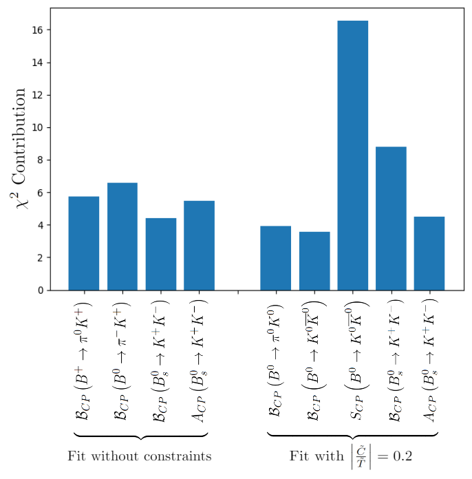
Figure 1: Observables providing the largest $\chi^{2}$ contributions for the global fits with $|{\widetilde{C}}/{\widetilde{T}}|$ unconstrained (left) and $|{\widetilde{C}}/{\widetilde{T}}|=0.2$ (right).

As we have seen, in the global fit to both $\Delta S=0$ and $\Delta S=1$ decays, the discrepancy with the SM is $3.6\sigma$ if $|{\widetilde{C}}/{\widetilde{T}}|$ is unconstrained, and it jumps to $4.4\sigma$ if $|{\widetilde{C}}/{\widetilde{T}}|$ is fixed to be 0.2. In Fig. 1, we identify the observables that contribute the most to the $\chi^{2}$ of each of these fits. On the whole, the large-$\chi^{2}$ observables are different for the two fits; the only ones that are important for both fits are the CP-averaged branching ratio and direct CP asymmetry of $B_{s}^{0}\to K^{+}K^{-}$. (This decay was identified as problematic in Ref. [3].) We also note that $\Delta S=1$ decays play an important role in these discrepancies. Perhaps there is a connection with the semileptonic $b\to s\ell^{+}\ell^{-}$ anomalies.

To sum up, assuming unbroken flavor SU(3) symmetry, a global fit to all $B\to PP$ data finds a discrepancy with the SM at the level of $3.6\sigma$. This discrepancy can be removed by allowing for SU(3)_F-breaking effects, but 1000% SU(3)_F breaking is required, i.e., parameters that are equal in the SU(3)_F limit must now differ by a factor of ten. These results are group-theoretically rigorous – no dynamical assumptions have been made. But if one also requires that $|C/T|=0.2$, which is the predicted value in QCD factorization, the discrepancy with the SM grows to $4.4\sigma$. These are the anomalies in hadronic $B$ decays. They strongly hint that new physics is present in these decays.

Acknowledgments: This work was financially supported by NSERC of Canada (RB, RB, AJ, SK, DL) and by the National Science Foundation, Grant No. PHY-2310627 (BB).