Towards out-of-distribution generalization in large-scale astronomical surveys: robust networks learn similar representations

Abstract

The generalization of machine learning (ML) models to out-of-distribution (OOD) examples remains a key challenge in extracting information from upcoming astronomical surveys. Interpretability approaches are a natural way to gain insights into the OOD generalization problem. We use Centered Kernel Alignment (CKA), a similarity measure metric of neural network representations, to examine the relationship between representation similarity and performance of pre-trained Convolutional Neural Networks (CNNs) on the CAMELS Multifield Dataset. We find that when models are robust to a distribution shift, they produce substantially different representations across their layers on OOD data. However, when they fail to generalize, these representations change less from layer to layer on OOD data. We discuss the potential application of similarity representation in guiding model design, training strategy, and mitigating the OOD problem by incorporating CKA as an inductive bias during training.

1 Introduction

Although the astronomy and cosmology communities have embraced ML methods, many key challenges remain. We focus on two such goals: the interpretability of ML models and their robustness under distribution shifts.

Robustness is particularly salient in astronomy because simulations only provide an approximate realization of the observed universe. In addition, different simulation models provide different realizations of the same astrophysical observables, so models trained on simulations from one environment may not generalize to simulations from another. A model that fails under a distribution shift between simulations may also fail when provided with real-world data, so it is crucial to assess whether a model is robust to a given distribution shift. A better understanding of the settings under which a model fails to generalize may guide us toward better OOD generalization. Better interpretations of ML models may also allow us to discover new hidden features within trained models, which hold significant importance in astronomy [1].

Recently, astronomy research has begun to apply interpretability techniques from machine learning. Matilla et al. [2] used saliency methods to interpret deep learning models trained to recover cosmological parameters from weak lensing maps. Morice-Atkinson et al. [3] used latent tree structures to analyze the relationship between model performance and data. Wu [4] used the Gradient-weighted Class Activation Mapping attribution tool to interpret the connection between galaxies’ morphological features and gas content. Cranmer [5] proposed using symbolic regression to discover mathematical expressions that approximate neural networks.

Cianfarani et al. [6] applied CKA to study robustness to adversarial examples, and we similarly consider the relationship between robustness and similarity in our setting. Specifically, we compare similarities of the internal representations of pre-trained CNNs using CKA, finding that when models fail to generalize under distribution shift, they tend to produce representations that remain similar between layers. We then discuss the possible connection between representation similarities and accuracy and how these insights can be used to promote robustness under distribution shift, suggesting ways to improve model training or prune neural network architectures.

2 Methods

2.1 Data

We use the publicly available CAMELS Multifield Dataset (CMD) [7], which is an open-access collection of 2D maps and 3D grids of 13 different fields created using different hydrodynamic (IllustrisTNG–henceforth, TNG, and SIMBA) and pure $N$-body simulations as part of the CAMELS project [8]. We here use 2D maps with $256\times 256$ pixels and size $25\,{\rm Mpc}/h$ of the total matter density (Mtot) and Gas temperature (Temperature) from the TNG and SIMBA simulations at $z=0$. The total matter density constitutes baryonic and dark matter contributions. The CMD dataset contains 1,000 simulations with 15 distinct maps per simulation.

2.2 CKA similarity measure

CKA compares the representations produced by different layers of the same or different architectures on shared input data. CKA is the normalized version of the Hilbert-Schmidt Independence Criterion (HSIC), which is used to test the dependence on distributions. Such a normalization allows the CKA metric to be invariant under isotropic scaling of the representations. The steps to compute CKA (assuming a linear kernel) are as follows (see Kornblith et al. [9] for more details). The input to CKA is a pair of representations $X\in\mathbb{R}^{m\times n_{X}}$ and $Y\in\mathbb{R}^{m\times n_{Y}}$ where $m$ is the number of examples and $n_{X},n_{Y}$ are the respective feature dimensions. These inputs are transformed into gram matrices denoted by $K$ and $L$ satisfying $K=XX^{T}$ and $L=YY^{T}$, such that $K$ and $L$ have shape $m\times m$. The resulting gram matrices are then centered using a centering matrix, $H=I_{n}-\dfrac{1}{n}11^{T}$, to produce $K^{\prime}=HKH$, $L^{\prime}=HLH$. Since CKA is the normalized version of the HSIC metric, the HSIC is first calculated by taking the dot product between the flattened versions of the centered gram matrices: $\textrm{HSIC}(K,L)=\dfrac{\textrm{vec}(K^{\prime})\cdot\textrm{vec}(L^{\prime})}{(m-1)^{2}},$ where vec transforms the matrix into a vector. The CKA is given by $\textrm{CKA}(K,L)=\dfrac{\textrm{HSIC}(K,L)}{\sqrt{\textrm{HSIC}(K,K)\textrm{HSIC}(L,L)}}.$ Following Nguyen et al. [10], we use the mini-batch CKA approach to reduce computational expense.

2.3 Implementation

Our CKA implementation closely follows Nguyen et al. [10]. The CKA calculation is performed on publicly available pre-trained CNNs on the CMD datasets from Villaescusa-Navarro et al. [11]. The basic architecture of these pre-trained CNN models consists of a series of blocks of convolutional layers $\rightarrow$ BatchNorm $\rightarrow$ Leaky ReLU layers followed by two fully connected layers with dropout. These CNNs were trained to predict the six cosmological and astrophysical parameters. We select the “best” trial based on validation loss, following the approach of [12] for calculating the CKA similarities using 50 maps for each field. A forward pass of the pre-trained CNN is performed on the test set two times independently, and the CKA similarity of each layer’s output representation (from the first pass) is computed for every layer’s output representation (from the second pass), yielding a CKA matrix.

To test the possible correlation between CKA similarities and performance, we compute the coefficient of determination $R^{2}$ score between the estimated and the true parameters. We only focus on recovering the cosmological parameters, $\Omega_{m}$ and $\sigma_{8}$, since most CNNs can marginalize over the astrophysics.

3 Results

We will refer to train-test setting pairs by name, e.g., TNG–SIMBA for the case where the CNN is trained on maps from TNG and tested on maps from SIMBA. We consider four cases to compute the CKA similarity matrices: TNG–TNG and TNG–SIMBA for Temperature maps, and SIMBA–SIMBA and SIMBA–TNG for Mtot.

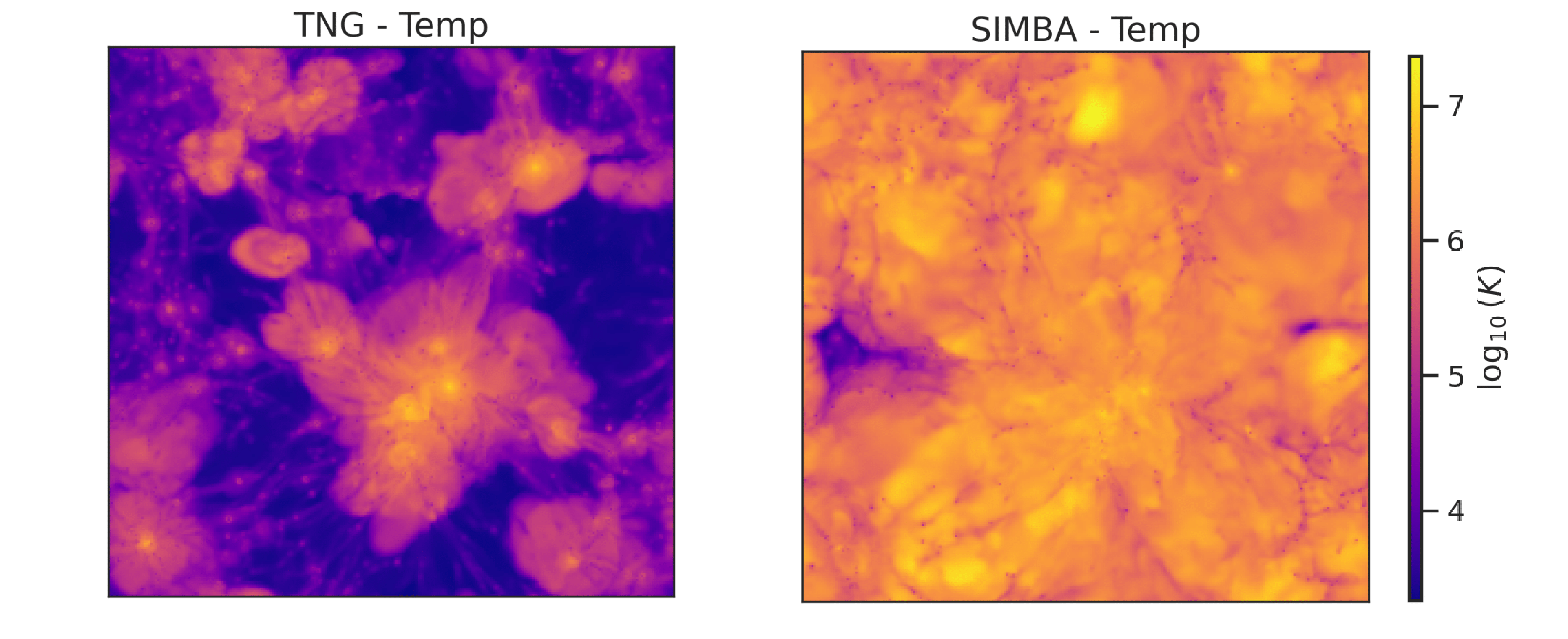
(a) Random example of the Temperature field from the TNG and SIMBA simulations.

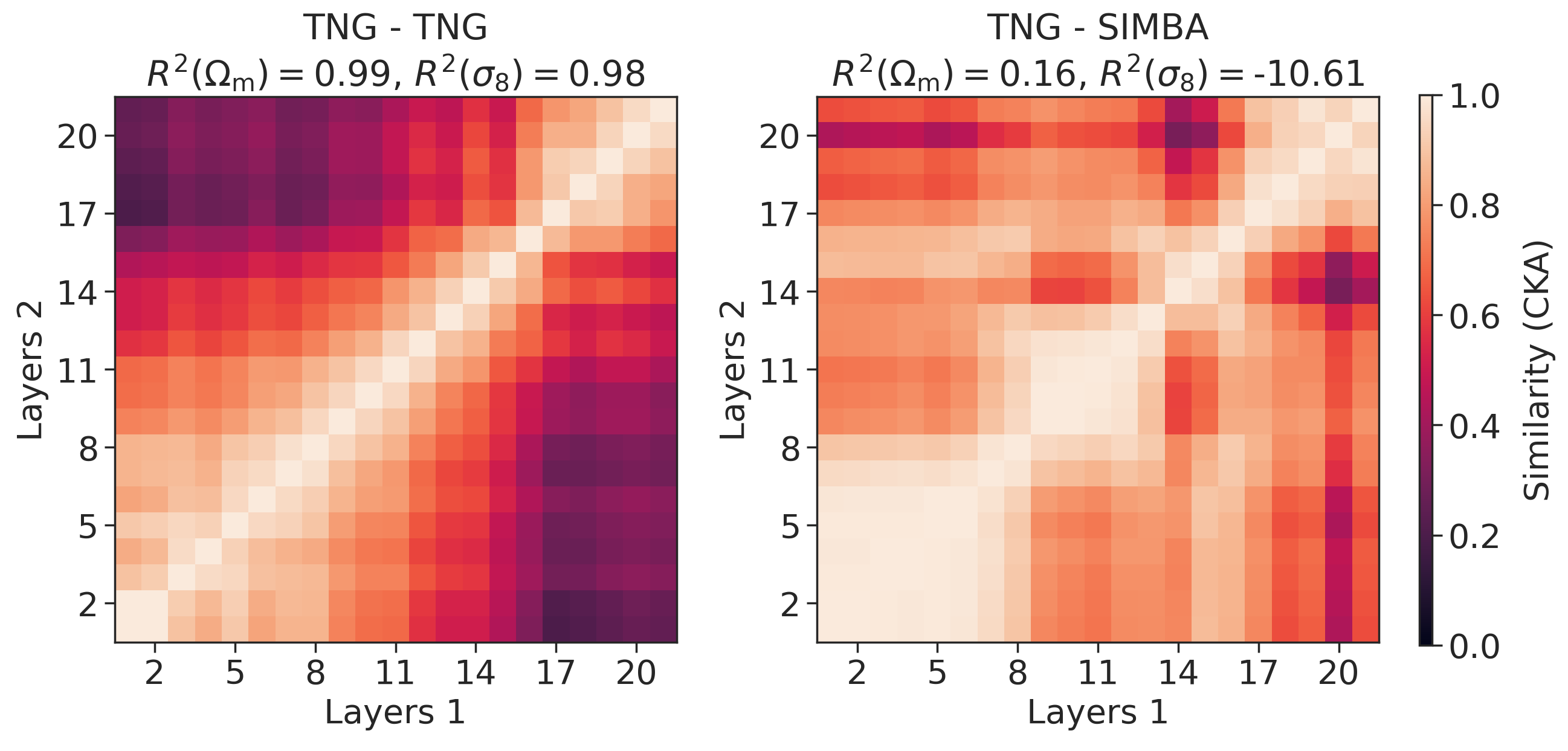
(b) CKA matrices for the ID (TNG-TNG) (left) and OOD (TNG-SIMBA) (right) cases. The titles show $R^{2}$ scores between model prediction and true value for the $\Omega_{\rm m}$ and $\sigma_{8}$ cosmological parameters.

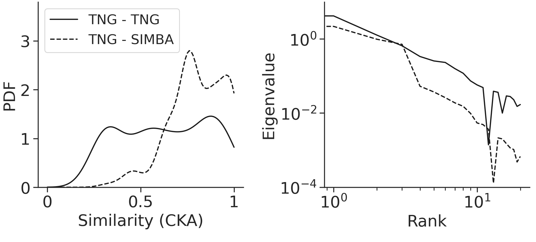
(c) Summary statistics of the CKA matrices from Fig. 1(b). On the left is the probability density function (PDF) of the CKA similarities, and on the right is the eigenvalues as a function of rank (i.e., the spectrum).

Figure 1: Analysis of the CKA similarities for the Temperature field. Representations of layers of the CNN trained on the TNG simulations are diverse only when the CNN is tested on 2D maps from TNG (i.e., ID samples) but are almost stagnant on 2D maps from SIMBA (i.e., OOD samples). The $R^{2}$ scores for TNG-SIMBA are drastically inferior to those for TNG-TNG, suggesting that the model fails to generalize to OOD (SIMBA) data.

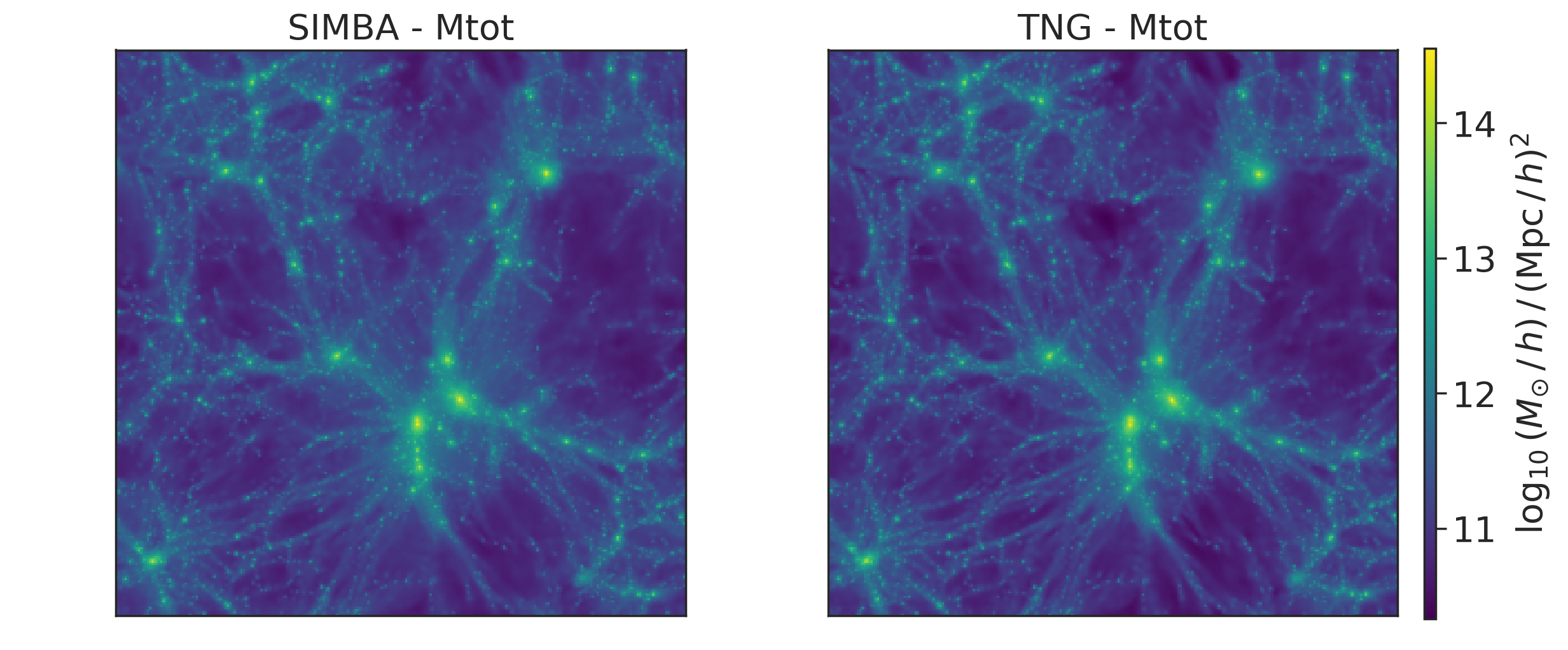
(d) Random example of the Mtot field from the SIMBA and TNG simulations.

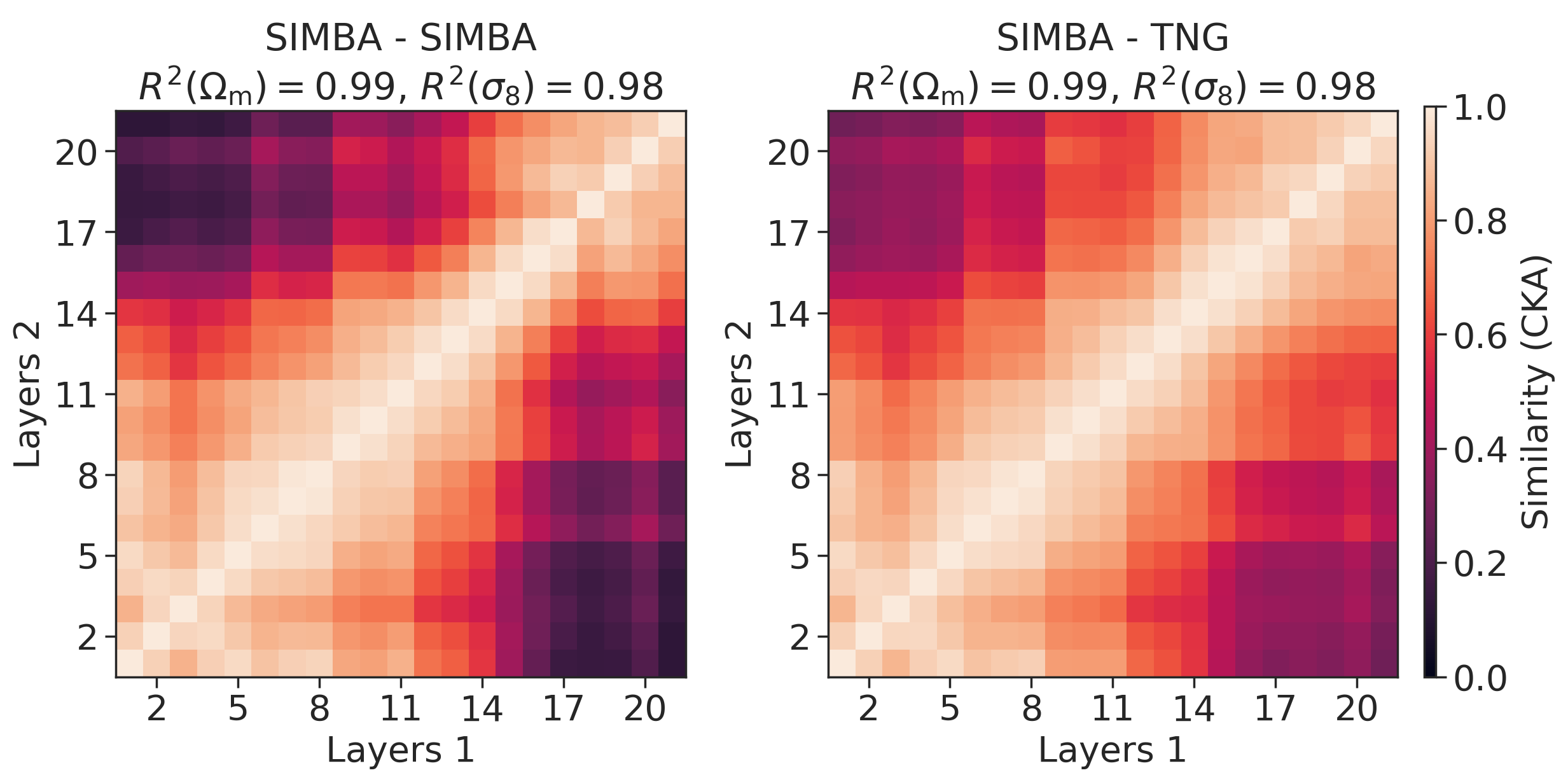
(e) CKA matrices for the ID (SIMBA-SIMBA) (left) and OOD (SIMBA-TNG) (right) cases. The titles show $R^{2}$ scores between model prediction and true value for the $\Omega_{\rm m}$ and $\sigma_{8}$ cosmological parameters.

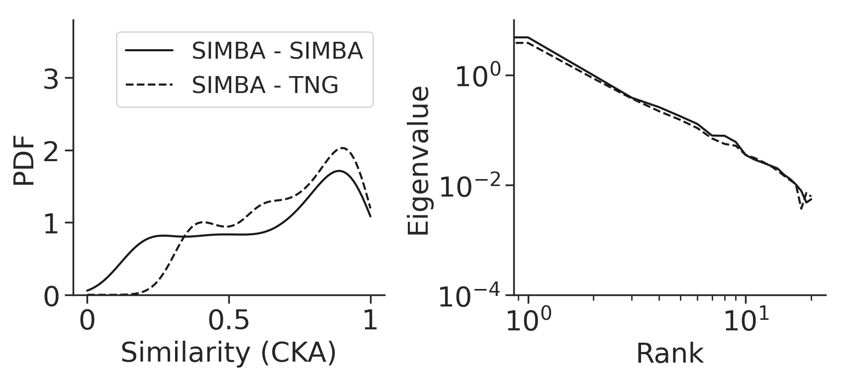
(f) Summary statistics of the CKA matrices from Fig. 1(e). On the left is the probability density function (PDF) of the CKA similarities, and on the right is the eigenvalues as a function of rank (i.e., the spectrum).

Figure 2: Analysis of the CKA similarities for the Mtot field. Representations of layers of the CNN trained on the SIMBA simulations are diverse not only when the CNN is tested on 2D maps from SIMBA (i.e., ID samples) but also when tested on 2D maps from TNG (i.e., OOD samples). The $R^{2}$ scores for SIMBA-TNG are the same as SIMBA-SIMBA, suggesting that the model robustly generalizes to OOD (TNG) data.

3.1 When a model fails to generalize OOD, outputs of different layers are similar

For the Temperature field, the model fails to generalize from the training simulation environment, TNG, to the OOD simulation environment, SIMBA. This failure to generalize is because while $R^{2}$ scores for the cosmological parameters ($\Omega_{m}$, $\sigma_{8}$) for TNG–TNG are high (0.99 for $\Omega_{m}$, 0.98 for $\sigma_{8}$), they deteriorate for TNG–SIMBA (0.16 for $\Omega_{m}$, -10.61 for $\sigma_{8}$).

The CKA matrices for TNG–TNG and TNG–SIMBA shown in Fig. 1(b) show a perfect similarity (= 1.0) along the main diagonal (i.e., bottom-left to top-right of the CKA matrix), which is expected since the scores on the diagonal compare each layer’s representation with itself. However, the similarities in the non-diagonal entries for the ID setting TNG–TNG are much smaller than those of the OOD setting TNG–SIMBA, which exhibits a block structure. The block structures for TNG–SIMBA indicate that different layers of the model produce similar representations on OOD inputs. In other words, the representations change only slightly as the OOD samples evolve deeper into this network.

We also quantify the differences in off-diagonal similarities in the CKA matrix that use ID and OOD data. The summary statistics (Fig. 1(c)) empirically show that the following hold for CKA matrices containing block structures compared to matrices without dominant block or diffused structures: (a) the distribution of the CKA similarities is more skewed towards larger values, and (b) their eigenvalues are smaller. The latter implies that the high CKA similarities are dispersed throughout the matrix rather than being dominantly focused on the diagonal, leading to smaller eigenvalues.

3.2 When a model successfully generalizes OOD, outputs of different layers are dissimilar

In the previous section, we illustrated how CKA similarities change between ID and OOD data for models that generalize poorly between simulations. We repeat the CKA analysis on models trained on the Mtot maps, which can successfully generalize between simulations. For the Mtot field, the $R^{2}$ scores for the cosmological parameters ($\Omega_{m}$, $\sigma_{8}$) in the ID setting SIMBA–SIMBA are high (0.99 for $\Omega_{m}$, 0.98 for $\sigma_{8}$). The $R^{2}$ scores remain identical for the OOD test setting SIMBA–TNG (0.99 for $\Omega_{m}$, 0.98 for $\sigma_{8}$). Therefore, the model is robust to the change in the simulation environment, perhaps partly because the shift appears smaller (Fig. 1(d)).

In contrast to Temperature, the CKA matrices for ID (SIMBA–SIMBA) and OOD (SIMBA–TNG) are similar visually (Fig. 1(e)). Although the block structures in the CKA matrix may not have been entirely removed for SIMBA–TNG, the representations of initial (1–5) and final (16–20) layers have become less similar than in the CKA of the OOD setting of Temperature (TNG–SIMBA; see Fig. 1(b)). In the Mtot setting, therefore, representations at the final layers have been substantially modified compared to those in the initial layers, standing in stark contrast to the behavior of a model during an OOD generalization failure as seen in Fig. 1(b).

Unlike Fig. 1(c), the summary statistics in Fig. 1(f) show that the eigenvalues and the distribution of the CKA similarities are similar for ID and OOD cases. These statistics quantify the visual differences between CKA matrices containing block structures and those that do not contain block structures. Overall, our experiments show that models produce different outputs at each layer when successfully generalizing OOD, but not when failing to generalize.

4 Conclusion and future work

Studying the CKA matrices of pre-trained CNNs tested using ID and OOD samples, we find that poor test-time model accuracy corresponds to higher similarity between different layers of the model (non-diagonal entries in the CKA matrix).

A high-similarity block feature in the CKA matrix suggests that these layers are unnecessary, and a similar accuracy can be obtained by replacing these layers with a single layer and then performing the training. In future work, therefore, the CKA matrix can be used to prune layers that correspond to diffused or block structures, which could reduce the memory footprint of the models while maintaining similar test-time performance. In addition, we have found that robust models have a characteristic feature of modifying their representations across different layers, whereas non-robust models possess stagnancy in their representations across different layers. This observation is crucial to the OOD generalization problem.

Our approach may be used to decide what simulations are best to train models for application on real-world data. By identifying when the model is not robust to a distribution shift, one can select data most similar to the OOD setting and produce novel training datasets capturing distribution shifts. Identifying generalization failures in this way is one method to build generally robust models, serving as feedback for improving training strategies to achieve OOD generalization. By understanding model behavior when failing to generalize, we can measure model confidence at test time and identify problem areas for learned models.

Future work can also investigate the causal impact of similarity structures on generalization performance in more detail. We plan to optimize these models by including the CKA matrix, as inductive bias, in the loss function to enforce similarity between CKA matrices of the ID and OOD samples, hence achieving OOD generalization. The advantage of this approach is that the computation of the CKA matrix does not require knowledge of physical parameters. This mimics the scenario of extracting information from real observations, where physical parameters are always unknown.

References

- Ntampaka et al. [2021] Michelle Ntampaka, Matthew Ho, and Brian Nord. Building Trustworthy Machine Learning Models for Astronomy. arXiv e-prints, art. arXiv:2111.14566, November 2021. doi: 10.48550/arXiv.2111.14566.
- Matilla et al. [2020] José Manuel Zorrilla Matilla, Manasi Sharma, Daniel Hsu, and Zoltán Haiman. Interpreting deep learning models for weak lensing. Phys. Rev. D, 102:123506, Dec 2020. doi: 10.1103/PhysRevD.102.123506. URL https://link.aps.org/doi/10.1103/PhysRevD.102.123506.
- Morice-Atkinson et al. [2018] Xan Morice-Atkinson, Ben Hoyle, and David Bacon. Learning from the machine: interpreting machine learning algorithms for point- and extended-source classification. Monthly Notices of the Royal Astronomical Society, 481(3):4194–4205, 09 2018. ISSN 0035-8711. doi: 10.1093/mnras/sty2575. URL https://doi.org/10.1093/mnras/sty2575.
- Wu [2020] John F. Wu. Connecting optical morphology, environment, and h i mass fraction for low-redshift galaxies using deep learning. The Astrophysical Journal, 900(2):142, sep 2020. doi: 10.3847/1538-4357/abacbb. URL https://dx.doi.org/10.3847/1538-4357/abacbb.
- Cranmer [2023] Miles Cranmer. Interpretable Machine Learning for Science with PySR and SymbolicRegression.jl. arXiv e-prints, art. arXiv:2305.01582, May 2023. doi: 10.48550/arXiv.2305.01582.
- Cianfarani et al. [2022] Christian Cianfarani, Arjun Nitin Bhagoji, Vikash Sehwag, Ben Y. Zhao, Prateek Mittal, and Haitao Zheng. Understanding Robust Learning through the Lens of Representation Similarities. arXiv e-prints, art. arXiv:2206.09868, June 2022. doi: 10.48550/arXiv.2206.09868.
- Villaescusa-Navarro et al. [2021a] Francisco Villaescusa-Navarro, Shy Genel, Daniel Angles-Alcazar, Leander Thiele, Romeel Dave, Desika Narayanan, Andrina Nicola, Yin Li, Pablo Villanueva-Domingo, Benjamin Wandelt, David N. Spergel, Rachel S. Somerville, Jose Manuel Zorrilla Matilla, Faizan G. Mohammad, Sultan Hassan, Helen Shao, Digvijay Wadekar, Michael Eickenberg, Kaze W. K. Wong, Gabriella Contardo, Yongseok Jo, Emily Moser, Erwin T. Lau, Luis Fernando Machado Poletti Valle, Lucia A. Perez, Daisuke Nagai, Nicholas Battaglia, and Mark Vogelsberger. The CAMELS Multifield Dataset: Learning the Universe’s Fundamental Parameters with Artificial Intelligence. arXiv e-prints, art. arXiv:2109.10915, September 2021a.
- Villaescusa-Navarro et al. [2021b] Francisco Villaescusa-Navarro, Daniel Anglés-Alcázar, Shy Genel, David N. Spergel, Rachel S. Somerville, Romeel Dave, Annalisa Pillepich, Lars Hernquist, Dylan Nelson, Paul Torrey, Desika Narayanan, Yin Li, Oliver Philcox, Valentina La Torre, Ana Maria Delgado, Shirley Ho, Sultan Hassan, Blakesley Burkhart, Digvijay Wadekar, Nicholas Battaglia, Gabriella Contardo, and Greg L. Bryan. The CAMELS Project: Cosmology and Astrophysics with Machine-learning Simulations. Astrophysical Journal, 915(1):71, July 2021b. doi: 10.3847/1538-4357/abf7ba.
- Kornblith et al. [2019] Simon Kornblith, Mohammad Norouzi, Honglak Lee, and Geoffrey Hinton. Similarity of Neural Network Representations Revisited. arXiv e-prints, art. arXiv:1905.00414, May 2019. doi: 10.48550/arXiv.1905.00414.
- Nguyen et al. [2021] Thao Nguyen, Maithra Raghu, and Simon Kornblith. Do wide and deep networks learn the same things? uncovering how neural network representations vary with width and depth, 2021.
- Villaescusa-Navarro et al. [2021c] Francisco Villaescusa-Navarro, Daniel Anglés-Alcázar, Shy Genel, David N. Spergel, Yin Li, Benjamin Wandelt, Andrina Nicola, Leander Thiele, Sultan Hassan, Jose Manuel Zorrilla Matilla, Desika Narayanan, Romeel Dave, and Mark Vogelsberger. Multifield Cosmology with Artificial Intelligence. arXiv e-prints, art. arXiv:2109.09747, September 2021c. doi: 10.48550/arXiv.2109.09747.
- Villaescusa-Navarro et al. [2022] Francisco Villaescusa-Navarro, Shy Genel, Daniel Anglés-Alcázar, Leander Thiele, Romeel Dave, Desika Narayanan, Andrina Nicola, Yin Li, Pablo Villanueva-Domingo, Benjamin Wandelt, David N. Spergel, Rachel S. Somerville, Jose Manuel Zorrilla Matilla, Faizan G. Mohammad, Sultan Hassan, Helen Shao, Digvijay Wadekar, Michael Eickenberg, Kaze W. K. Wong, Gabriella Contardo, Yongseok Jo, Emily Moser, Erwin T. Lau, Luis Fernando Machado Poletti Valle, Lucia A. Perez, Daisuke Nagai, Nicholas Battaglia, and Mark Vogelsberger. The camels multifield data set: Learning the universe’s fundamental parameters with artificial intelligence. The Astrophysical Journal Supplement Series, 259(2):61, apr 2022. doi: 10.3847/1538-4365/ac5ab0. URL https://dx.doi.org/10.3847/1538-4365/ac5ab0.