GausSN: Bayesian Time-Delay Estimation for Strongly Lensed Supernovae
Abstract
We present GausSN, a Bayesian semi-parametric Gaussian Process (GP) model for time-delay estimation with resolved systems of gravitationally lensed supernovae (glSNe). GausSN models the underlying light curve non-parametrically using a GP. Without assuming a template light curve for each SN type, GausSN fits for the time delays of all images using data in any number of wavelength filters simultaneously. We also introduce a novel time-varying magnification model to capture the effects of microlensing alongside time-delay estimation. In this analysis, we model the time-varying relative magnification as a sigmoid function, as well as a constant for comparison to existing time-delay estimation approaches. We demonstrate that GausSN provides robust time-delay estimates for simulations of glSNe from the Nancy Grace Roman Space Telescope and the Vera C. Rubin Observatory’s Legacy Survey of Space and Time (Rubin-LSST). We find that up to 43.6% of time-delay estimates from Roman and 52.9% from Rubin-LSST have fractional errors of less than 5%. We then apply GausSN to SN Refsdal and find the time delay for the fifth image is consistent with the original analysis, regardless of microlensing treatment. Therefore, GausSN maintains the level of precision and accuracy achieved by existing time-delay extraction methods with fewer assumptions about the underlying shape of the light curve than template-based approaches, while incorporating microlensing into the statistical error budget rather than requiring post-processing to account for its systematic uncertainty. GausSN is scalable for time-delay cosmography analyses given current projections of glSNe discovery rates from Rubin-LSST and Roman.
keywords:
gravitational lensing: strong – gravitational lensing: micro – methods: statistical – supernovae: general – supernovae: individual: SN Refsdal – distance scale1 Introduction
Strong lensing of a background variable source, such as a supernova (SN), by a foreground galaxy or galaxy cluster, can result in the appearance of multiple images of the source. Refsdal (1964) was the first to demonstrate that the time delay between the multiple images of a gravitationally lensed supernova (glSN) images could be related to when combined with a model of the lens mass distribution. A independent estimate from strong lensing is motivated by the persistent tension between the present-day expansion rate of the universe, , measured using light from early-times (i.e. the Cosmic Microwave Background; Planck Collaboration et al., 2020) and from late-times (i.e. the distance ladder; Riess et al., 2022), known as the Hubble tension. If determined to be physical, this tension may be suggestive of new physics beyond our present model of the universe, CDM (Mörtsell & Dhawan, 2018; Di Valentino et al., 2021). As time-delay distances inferred from strong lensing are completely independent of the luminosity distances used in the distance ladder, time-delay cosmography represents a promising technique for cross-checking local measurements of (see e.g. Treu et al., 2022; Suyu et al., 2023 for recent reviews). In this paper, we present GausSN: a Bayesian semi-parametric approach for the extraction of time delays from glSN systems using Gaussian Processes (GPs). GausSN is a publicly available package that can be found at: https://github.com/erinhay/gaussn.
Because of the rarity of glSNe, the first cosmological constraints from strong lensing came from quasars (e.g. Keeton & Kochanek, 1997; Wong et al., 2020; Birrer et al., 2020). However, SNe have several advantages over quasars for strong lensing analyses which have the potential to push the field further in precision and accuracy. Firstly, that SNe disappear after a few months allows for the study of the lens and host galaxy in greater detail. Improved knowledge of the lens helps to break the mass-sheet degeneracy (Falco et al., 1985), which was cited as the main source of uncertainty in the H0LiCOW estimate of (Wong et al., 2020; Birrer et al., 2020). If the lensed object is a Type Ia supernova (SN Ia), further leverage can be gained from the fact that SNe Ia are standardizable candles (Foxley-Marrable et al., 2018; Birrer et al., 2022). Secondly, the relatively simple light curves of SNe, in contrast to the stochastic variability of quasars, makes it easier to extract time delays from the systems. The single peak in brightness limits the degeneracies in matching the images. Furthermore, for SNe Ia, the well-known light curve shapes and colour distributions can help to constrain the effects of microlensing and dust extinction on the system. Microlensing can distort the shape of an image’s light curve and lead to artificial shifts in the apparent peak of the light curve – a “microlensing time-delay” (Bonvin et al., 2019a). This effect has proven to be a difficult effect to disentangle from underlying variability from the source (Foxley-Marrable et al., 2018; Pierel et al., 2023). Time-delay estimation with glSNe can also be done with a shorter time frame of observations because their variability is constrained to a period of a few weeks to months, compared to the years required for measure reliable time delays from lensed quasars (Bonvin et al., 2017, 2018, 2019b). Of course, the rarity of SNe and short window in which they are active make glSNe more difficult to discover.
Therefore, it was not until November 2014 that the first cosmologically useful glSN, SN Refsdal, was discovered (Kelly et al., 2015). SN Refsdal, a peculiar Type II SN at (Kelly et al., 2016b), was discovered with four images in an Einstein cross due to lensing by an elliptical galaxy in the MACS J1149.6+2223 galaxy cluster at . Unfortunately, the time delays from galaxy-scale lensing, originally estimated in (Rodney et al., 2016), were determined to be too short and imprecise to obtain a measurement of . However, the host galaxy of SN Refsdal was also imaged multiple times. It was predicted that a image of SN Refsdal would later appear in another image of the host galaxy with a time delay of just under a year (Kelly et al., 2015; Oguri, 2015; Sharon & Johnson, 2015; Grillo et al., 2016; Diego et al., 2016; Jauzac et al., 2016; Kawamata et al., 2016; Treu et al., 2016). As predicted, SN Refsdal reappeared less than a year later in October 2015 (Kelly et al., 2016a). Using the time delay between SN Refsdal’s fifth image and the other four images (Kelly et al., 2023b), the first measurement of was published in May 2023 (Kelly et al., 2023a). Finding – a 6.0% precision estimate – SN Refsdal alone has demonstrated the importance of glSNe as precise local cosmological probes.
In addition to SN Refsdal, seven glSNe have been found: SN PS1-10afx (Chornock et al., 2013; Quimby et al., 2013), SN 2016geu (Goobar et al., 2017), SN Requiem (Rodney et al., 2021), SN C22 (Chen et al., 2022), SN Zwicky (Goobar et al., 2023a), SN 2022riv (Kelly et al., 2022), and SN H0pe (Frye et al., 2023b, a; Polletta et al., 2023). However, SN Refsdal has been the only one of these eight that has been used for cosmology thus far. Six of the others have suffered from either having extremely short time delays (SN 2016geu’s, SN Zwicky’s, and some of SN Requiem’s images have time delays of only a few hours), having extremely long time delays (SN Requiem’s final image is expected to reappear in 2037), being found only in an archival search and therefore having insufficient data (SN PS1-10afx, SN Requiem, and SN C22), or having only one observed image (SN 2022riv). SN H0pe, recently discovered in March 2023, is a strong candidate for a second glSN measurement of . Analysis of SN H0pe is currently ongoing and more information about this glSN is expected in the near future.
In the next decade, the Vera C. Rubin Observatory’s Legacy Survey of Space and Time (Rubin-LSST) and Roman Space Telescope (Roman) are expected to discover tens to hundreds of glSNe, if we adopt the right search strategies (Huber et al., 2019; Wojtak et al., 2019; Pierel et al., 2021; Craig et al., 2021). With this data, it will be possible to reach percent level constraints on the cosmological parameters competitive with SH0ES and Planck measurements (Huber et al., 2019, Arendse et. al., 2023, in prep). As samples of glSNe grow, so does their potential to resolve the Hubble tension with precise local measurements of .
The relatively simple and well-understood variability of SNe lends itself to time-delay estimation techniques based around SN light curve templates. In particular, template-based Supernova Time Delays (sntd; Pierel & Rodney, 2019) has emerged as the standard for glSNe time-delay estimation due to its flexibility and accessibility. The package is built upon sncosmo (Barbary et al., 2023), which contains a diverse library of SN light curve templates. In addition, a flexible Bazin function (Bazin et al., 2009) can be used as the underlying template, if spectroscopic classification is unavailable or ambiguous. Given a specified SN light curve template, sntd uses the nested sampling functionality available through sncosmo to yield posterior distributions for the light curve template parameters, the time delay, and the magnification.
However, uncertainties relating to template choice and the unknown redshift evolution of SN light curves, especially for types of SNe other than SNe Ia, may introduce systematic errors into the time-delay analysis that are difficult to quantify. While template-based approaches are motivated by the well-described nature of some SN light curves, a complementary method which is independent of these potential systematics is needed. GausSN is a template-independent approach for time-delay estimation that models the underlying light curve non-parametrically using a Gaussian Process (GP). This model is motivated by previous work on quasar time-delay estimation with GPs, in particular that of Tak et al. (2017), as well as that of Hojjati et al. (2013); Hojjati & Linder (2014); Meyer et al. (2023).
By modelling the underlying light curve non-parametrically with a GP, GausSN is able to fit the light curves of any type of SN without prior knowledge of the type or the redshift of the object. In addition, the model naturally fits for the time delays of all images, observed in any number of bands, simultaneously. By fitting all images in all filters together, we take advantage of the full information available from the data by leveraging the knowledge that for each band, the multiple images’ time-series are time-shifted and magnified realization of the same underlying light curve. GausSN also implements a novel microlensing treatment which occurs alongside time-delay estimation for a one-step time-delay measurement. A time-varying magnification term is used to account for both macrolensing and microlensing simultaneously with the time-delay estimate. Because the time delay and microlensing are jointly inferred, GausSN does not require post-processing to account for a systematic error budget due to microlensing, but instead incorporates uncertainty from microlensing in the statistical uncertainty. Therefore, GausSN provides a coherent Bayesian time-delay estimate in one-step, without the need for post-processing to account for systematics from template choice or microlensing.
The peculiar nature of SN Refsdal’s light curve exemplifies the need for a template-independent approach for time-delay estimation for glSNe, such as GausSN. Although most similar to SN 1987A (Woosley et al., 1988; Kelly et al., 2016b), SN Refsdal’s light curves are not well described by any existing templates (although some theoretical models have been developed, e.g. Baklanov et al., 2021). While the light curves of SNe Ia are highly uniform, the shapes of the light curves of other types of supernovae are less well studied and more highly varied from object to object. GPs are well suited for this application, as they are flexible and data driven, with minimal assumptions about the properties of the true underlying light curve.
Indeed, in the analysis of the time delays of SN Refsdal’s five images, the Bayesian Gaussian Process method, upon which GausSN is based, was highly successful (Kelly et al., 2023b). Four methods, including sntd and a custom piecewise polynomial template approach, were tested on simulations of SN Refsdal-like light curves to determine the quality of each method’s fits. In simulations, the Bayesian Gaussian Process method outperformed the template-based approaches for extracting the time delays of the 2 best-sampled images S2 and S3 relative to the first image. On the other hand, sntd and the custom template approach were more successful in estimating the time delay of the more poorly sampled images S4 and SX relative to the first image. Ultimately, the custom template was the most generally successful in fitting for time delays and magnifications for all the images in simulations.
GausSN provides coherent Bayesian time-delay estimates with complementary strengths to existing template-based time-delay estimation methods. As a template-independent approach, GausSN does not require prior knowledge of SN type or redshift, making the model quick and easy to implement. Furthermore, GausSN is not subject to potential sources of systematic uncertainties and biases from template choice; fine tuning of generic SN templates, such as the Bazin function; or the need to construct custom templates, which may not be feasible for larger samples of glSNe and makes validation of an analysis difficult. Finally, the model provides Bayesian time-delay estimates in one step, without the need for post-processing to account for systematic uncertainty from microlensing, by incorporating a time-varying magnification treatment.
In §2, we describe how we model glSN in flux-space with GPs. We describe the microlensing model in §3 and the sampling algorithms implemented in GausSN in §4. In §5, we show the fits to simulated doubly-imaged glSN light curves as expected to be seen from Rubin-LSST and Roman. We then apply GausSN to the five images of SN Refsdal in §6. In §7, we discuss the performance of GausSN compared to other leading time-delay extraction techniques, as well as comment on future work possible with GausSN. In §8, we conclude.
2 Modelling glSNe with Gaussian Processes in Flux-Space
Strong lensing of a supernova by a foreground galaxy or galaxy cluster results in the appearance of multiple images, which are copies of the same underlying light curve. These multiple images are observed with some shift in time and magnification or de-magnification relative to each another. We model the true underlying light curve in flux space, , as a draw from a Gaussian Process:
| (1) |
where is the mean function, which can depend on time, t, in the case of time series data, and is the covariance (or kernel) function, which gives the covariance between and .
Throughout this work, we use a zero mean function, such that . The zero mean function encourages the inferred function to go to zero flux outside of where there is data, which reflects the physical expectation that before and after the SN explosion, we expect an average of zero background-subtracted flux. For the covariance function, we choose the squared exponential kernel:
| (2) |
where , the amplitude, and , the length scale, are the two hyperparameters controlling the kernel. This kernel enforces strong correlation between points nearby to one another, with weaker correlation as points further away are considered. It is also stationary, or invariant to overall time shifts, and produces smooth functions (Rasmussen & Williams, 2006). The squared exponential kernel has proven to be well-suited for fitting SN light curve data, as it has been used to do so in previous work with success (Kim et al., 2013; Boone, 2019; Vincenzi et al., 2019; Qu et al., 2021).
The GP is defined such that any vector consisting of the evaluations of this continuous function, , at the finite set of points, , has a joint multivariate Gaussian prior distribution:
| (3) |
where the elements of the covariance matrix, , are given by for . Note that we use to denote a multivariate normal vector with mean and covariance matrix . Then, gives the PDF of the vector.
2.1 Two Images in One Band
We first consider the simplest case of two images observed in one band, i.e. a filter covering a defined range of wavelengths. Taking image 1 to be the arbitrarily chosen reference image, the light curves of the two images are described by:
| (4) |
where is the relative time delay of image 2 compared to image 1 and is the relative magnification of image 2 compared to image 1.
Say we observe image 1 at a set of times, , and image 2 at a set of times, . We define and , the observations of image 1 and 2 respectively, such that for the observation of image 1:
| (5) | ||||
| (6) |
and for the observation of image 2:
| (7) | ||||
| (8) |
where and are the standard deviations of the measurement errors of image 1 and image 2, respectively. We assume that the measurement errors are independent. We re-scale the flux data and measurement standard deviations for each band and image by a single, constant factor determined by the range of fluxes over all images and bands.
We concatenate these two vectors to give the flux data vector, , as:
| (9) |
and the time data vector, , as:
| (10) |
In addition, we define the de-shifted time vector, , which depends on the time delay, :
| (11) |
To infer from the data and , we fit for a time delay, , and magnification, , in addition to the two kernel hyperparameters. Therefore, .
The marginal likelihood over is given as:
| (12) |
where we can think of in four quadrants:
| (13) |
Recall that for a GP, the covariance is given as . With Equations 5-8, the covariances in the first quadrant are:
| (14) |
assuming there is no covariance between and , as the physical process generating the light curve is independent of the measurement process. In the second quadrant, the covariances are:
| (15) |
It follows that:
| (16) |
and
| (17) |
for the remaining two quadrants. Because our choice of kernel is stationary, .
Based on this formulation, we can decompose into three factors:
| (18) |
where represents a Hadamard product (i.e. the elementwise product). The first factor, , depends only on . Defining as a matrix of ones, is given as:
| (19) |
where, again is the number of observations of image 1 and is the number of observations of image 2. The second factor, , depends on and the kernel parameters and is defined as:
| (20) |
where is the matrix whose element is . Finally, the diagonal matrix contains the variances of the measurement errors, , along the diagonal.
With a specified prior on and Equation 12, we can construct the posterior:
| (21) |
which we can sample from and marginalize over to determine the probability distributions over the parameters. The dependence of on arises because we will restrict the time delay, , to be within the range of observations.
2.2 Two Images in Two Bands
We will now consider the case with two images in two bands – band A and band B. We now have two functions we wish to model as a draw from a GP:
| (22) |
and
| (23) |
where the draws from the GP for each band are independent111While we choose to neglect correlations between the underlying light curves in different bands, these correlations can in principle be included, for example as in Hu & Tak (2020).. The light curves of the images are therefore defined by:
| (24) |
We note that the magnification and time delay of the second image relative to the first is the same in band A as it is in band B. Therefore, there is still only one and one for which to fit, so it remains that . It is possible to adopt unique GP kernel hyperparameters for each band, but we find that these extra parameters are unnecessary for the examples that follow in this paper.
We construct the flux data vector, , as:
| (25) |
and the time data vector, , as:
| (26) |
where are the observations of image in band at times . We also define the de-shifted time vector, , as:
| (27) |
The marginal likelihood is:
| (28) |
where, again, .
We make the simplifying assumption that there is no shared information between bands beyond the time delay and magnification. In other words, there is no covariance of either image in band A with either image in band B. With this in mind, we write as:
| (29) |
where denotes a matrix of all zeros and and are defined as in Equation 20 for each band separately. We point out that there does not need to be the same number of observations of the images in band A as there are in band B. Therefore, the shape of need not necessarily be square.
Finally, the posterior is the same in this case as in Equation 21 with the new marginal likelihood terms defined for this data case. The case of two images in two bands can be generalized to fit multiple () images in multiple () bands. We fit simulated multi-band data as expected from Rubin-LSST and Roman in §5 and multi-image data from SN Refsdal in §6.
3 Microlensing
The effect of microlensing from stars and substructure in the lensing galaxy or galaxy cluster can additionally introduce additional time-varying magnification to individual images. Microlensing in systems of glSNe is extremely difficult to model because of complex layouts of stars and dark substructure in the foreground of lensing systems. The discrepancy in the model-predicted brightnesses of the four images from SN Zwicky without considerations of microlensing and the observed brightnesses of the images – up to 1.5 mag for one image – demonstrates the difficulty of modeling this effect and the significant impact which microlensing/substructure can have on a system (Pierel et al., 2023; Goobar et al., 2023b).
Following Tak et al. (2017), we model microlensing as a time-dependent extension of , so the previously constant becomes . Because we can only learn relative magnification effects from the light curve data available, we take all magnification to be relative to an arbitrarily chosen image 1. Therefore, Equations 5-8 become:
| (30) | ||||
| (31) | ||||
| (32) | ||||
| (33) |
where again and are the standard deviations of the measurement errors of image 1 and image 2, respectively.
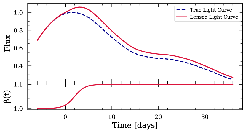
Figure 3 in Foxley-Marrable et al. (2018) and Figure 3 in Pierel et al. (2023) illustrate from microlensing maps examples of microlensing as a function of time. In these example microlensing curves, a period of constant magnification is typically interrupted by one change in brightness which occurs over a range of timescales, from less than a day to weeks. Physically, this shape corresponds to the SN crossing a microcaustic as the photosphere expands. After this change, the observed magnification appears to remain constant, as the small size of the SN and microlensing sub-structures means the photosphere most often crosses only one significant microcaustic. Therefore, we have chosen to model microlensing as a sigmoid function, given by:
| (34) |
where is the macrolensing effect, is the scale of the microlensing effect, is the rate of change in the microlensing effect, and is the location of a change in microlensing.
We make the simplifying assumption of achromatic microlensing, or microlensing which is identical across bands for a given image. It is demonstrated by Goldstein et al. (2018); Huber et al. (2021) that this assumption is valid for the first three rest-frame weeks of lensed SN Ia, in which time microlensing is predicted to be largely achromatic. This model for the time delay and magnification therefore takes 5 parameters per image. The parameters we fit for in a doubly-imaged system are now .
Consider again the case of two images observed in one band, where image 1 is observed at a set of times and image 2 is observed at a set of times. For this system, the matrix from Equation 19 is now:
| (35) |
where is a vector of ones of length and is a vector of length whose element is given by . This formulation generalizes to an arbitrary number of images observed in an arbitrary number of bands. We will refer to the model with a constant as the “constant magnification” model and the model with a time-varying magnification term as the “sigmoid magnification” model.
Figure 1 demonstrates how a time-varying magnification term can have a significant impact on the shape of a SN light curve, to the point that the inferred time delay could be significantly skewed if the glSN system is fit with a constant magnification model. A combined treatment of macrolensing and microlensing mitigates the potential source of bias that arises if these magnification effects are considered separately. We explore this effect in greater detail in Appendix A.
4 Sampling Algorithms
Within the publicly available GausSN framework, we implement three methods for sampling from the posterior distributions:
- •
- •
- •
We choose to sample parameters with dynesty for the analyses in this paper. The nested sampling approach is best able to handle the multi-modal nature of the posteriors on the time delay and other magnification parameters. Therefore, for the most accurate time-delay estimates and associated uncertainties, we opt for dynesty.
Within dynesty, we use both uniform sampling with multi-ellipsoidal bounding (Feroz et al., 2009), for systems with fewer than 100 data points and fewer than 5 parameters, and random slice sampling, for systems with more than 100 data points or more than 5 parameters, with 500 live points. The slice sampling technique was developed by Neal (2003) and first implemented within the nested sampling framework by Handley et al. (2015a, b). We retain the default stopping criteria in dynesty, which is met when the remaining, unaccounted for evidence is less than a threshold which depends on the number of live points used (Speagle, 2020). We note that the specifications of dynesty sampling, and all other sampling methods, can be easily adjusted within the GausSN parameter optimization function.
Given these specifications, GausSN performs as follows. For an object with 320 total data points, i.e. 40 observations of 2 images in 4 bands, a single evaluation of the marginal likelihood takes ms using standard CPU resources on a desktop computer. The stopping criteria is typically met after 200,000-800,000 evaluations of the likelihood function, which roughly corresponds to 5,000-15,000 nested sampling iterations. Therefore, the nested sampling algorithm takes between 5 and 30 minutes to run for such an object. Depending on the quantity and quality of the data, sampling may take anywhere from 30 s to an hour for the simulated Rubin-LSST and Roman data. Given the rarity of glSNe, even in the best case scenarios for future observatories, such run times will not be a barrier for future applications of our model to real data.
5 Tests on Simulated Data
5.1 Roman Simulations
5.1.1 Data
Recently, Pierel et al. (2021) (hereafter P21) simulated 2.4 million glSN light curves – 600,000 each of Type Ia, Ib/c, IIn, and IIP – as expected from the Roman Space Telescope.222Publicly available at: https://dx.doi.org/10.17909/t9-k8w7-zk32. The cadence, depth, and detection thresholds for the simulations are based on the Roman SN survey "All-z" strategy described in Hounsell et al. (2018), with modifications made for more recent survey updates. Based on the current plans for the instrument, P21 predicts Roman will discover glSNe up to .
The simulation pipeline works as follows: for each SN subclass, a sample of 50 simulated galaxy-scale lenses are used to simulate 10 distinct glSN light curves with 2-4 images based on the structure of the lens. Each of these 500 systems are then subject to 100 iterations of microlensing for each of 12 microlensing maps, yielding 1200 variations of each glSN light curve. P21 assumes achromatic microlensing, so any individual image experiences the same microlensing effects across wavelength space. The 12 microlensing maps are based on different choices of stellar mass model, which vary the effective radius, initial mass function, and Sérsic index of the galaxy profile. Objects are required to pass a series of data cuts, which are described in P21. For simplicity, we consider only the doubly-imaged glSNe from the P21 Roman simulations.
We fit each object with both the constant magnification model and the sigmoid magnification model. For the constant magnification model, we use the following priors on the two kernel parameters, the time delay, and the magnification333We use to denote a uniform distribution over (a, b) and to denote a truncated normal distribution where and are the mean and variance of an untruncated normal distribution, which is then truncated on the left at location and on the right at location .:
| (36) | |||
| (37) | |||
| (38) | |||
| (39) |
where is the difference between the times of the brightest observations of image 2 and 1 and is the ratio of the brightest observation of image 2 relative to the brightest observation of image 1. We define and to be all the times of observation of image 1 and 2, respectively. The prior on therefore requires that there always be overlap between data from image 1 and data from image 2. Although the scaled flux data has a maximum value of 1, we allow the prior on to range from 0 to 5 so as not to overly restrict the amplitude of the underlying light curve.
We adopt wide priors on all parameters to ensure the diversity of behavior present in the simulations is represented in our parameter space. With real glSN events, which will be fit on an individual basis because of their rarity, these priors can be adjusted to account for additional contextual information for each specific event.
5.1.2 Analysis
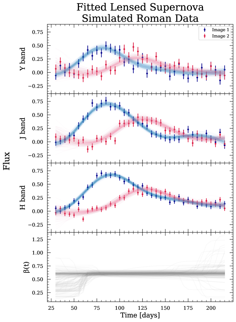
On an individual object basis, the GP fits to the data and posterior distributions show that GausSN is effectively and accurately inferring the time delays from the glSNe systems. In Figure 2, we demonstrate the quality of the fit on the light curve level from the sigmoid magnification model. We plot the observed data with draws from the posterior predictive distribution. The bottom panel of the figure shows realizations of the magnification function for each posterior sample. Notably, because we are only able to constrain the relative magnification, the magnification function shows greater uncertainty around the beginning and end of the time series because these regions are where the light curve lacks overlapping data from the two images.
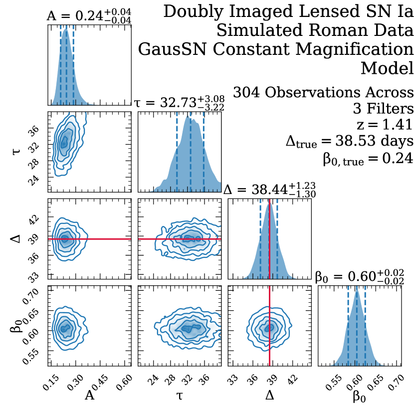
In Figure 3, we show the posteriors of the constant magnification fit. GausSN recovers days, whcih captures the true time delay of 38.53 days well within the 68% credible interval (CI). As we don’t necessarily expect the posteriors to be Gaussian, we calculate the 68% CI from the and percentiles of the posterior samples. The magnification is not well recovered, as GausSN finds , when the true . We attribute this discrepancy to the presence of microlensing from lens substructure. Indeed, there is more uncertainty in the recovered magnification when fitting with the sigmoid magnification model. With this model, GausSN finds , which is more consistent with the truth. The uncertainty on the time delay is however increased when fitting with the sigmoid magnification model, as expected, with . This represents a 5.22% precision time-delay estimate with the sigmoid magnification model, up from 3.38% precision with the constant magnification model. Of course, the constant magnification model gives only a statistical uncertainty, so it does not take into consideration systematic uncertainty from microlensing. A separate systematic microlensing error would have to be accounted for in post-processing. Therefore, the time delay estimate with the sigmoid magnification model may, in the end, be more precise.
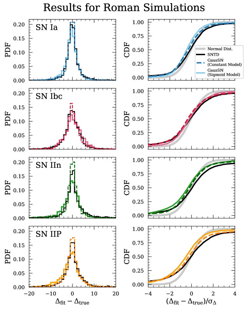
On a population level, GausSN performs well across all subclasses of SNe and mass models. We note that the true parameters for the SN IIP SC2 and SC4 mass models were not available, so these results are excluded from the reported statistics. The left column of Figure 4 shows the distribution of for the sigmoid and constant magnification models. We also compare to the results from sntd, which are included in the P21 simulated Roman data release. With the constant magnification model we find 35.32% of time delays within day, 70.33% within days, and 83.73% within days. With the sigmoid magnification model, we find that 27.13% of time delays are recovered within day, 62.12% are recovered within days and 79.07% are recovered within days. For comparison, sntd recovers 31.95% within day, 66.25% within days, and 81.28% within days.
We also consider the fractional error, , on the time-delay estimates. This metric gives a better sense of closeness to the truth scaled by the size of the time delay. For the constant magnification model, we find that 32.55% of systems have fractional errors of less than 5% and for the sigmoid magnification model, 26.48% of systems have fractional errors of less than 5%. These results are comparable to the sntd results, which find 30.84% of systems to have a fractional error of less than 5%.
GausSN, therefore, is effective at estimating time delays close in absolute and fractional value to the true time delay. That the sigmoid magnification model is in general further from the truth according to this metric than the constant magnification model or sntd is not unexpected. As this model has more flexibility, often leading to more complex posteriors, the point estimate for the time delay may be further from the truth. The full posteriors give a more accurate sense of the time-delay estimate by a given model.
In the right column of Figure 4, we show the CDF of the standardised error, distribution for the sigmoid and constant GausSN magnification models, sntd, and a unit normal distribution for reference. If the uncertainties are well-calibrated, we expect that across the sample of SNe, 68% of will fall within the 68% CI and 95% of will fall within the 95% CI. Although the full posterior distributions from sntd are not available, we can compare these statistics to the fraction of SNe which have time delays recovered within and of the truth from the sntd point estimate and uncertainty.
For the constant magnification model, we find 54.46% in 68% CI and 81.31% in 95% CI. For the sigmoid magnification model, we find 54.65% of SNe with in 68% CI and 82.65% in 95% CI. For sntd, 50.92% of SNe have which fall in the CI and 78.33% fall in the CI. While these statistics do not meet the benchmark set by the normal distribution, they are comparable to, if not a slight improvement on, the results from sntd. Therefore, GausSN provides time-delay estimates that are as close, if not closer, in absolute value to the truth with relatively well-calibrated uncertainties compared to sntd, the leading time-delay estimation technique for glSNe. As there are some variations for different types of SNe, we report the above statistics broken down by subclass of SN for all three models in Table 1.
| SN Type | Na | Model | < 1 day | < 3 days | < 5 days | < 5% | in 68% CIb | in 95% CIb |
|---|---|---|---|---|---|---|---|---|
| Ia | ||||||||
| 2340 | Sigmoid | 0.358 | 0.741 | 0.873 | 0.368 | 0.636 | 0.912 | |
| 2340 | Constant | 0.414 | 0.788 | 0.901 | 0.436 | 0.608 | 0.88 | |
| 2340 | SNTD | 0.381 | 0.762 | 0.884 | 0.437 | 0.588 | 0.853 | |
| 599901 | SNTD | 0.386 | 0.764 | 0.883 | 0.421 | 0.568 | 0.842 | |
| Ibc | ||||||||
| 2243 | Sigmoid | 0.226 | 0.572 | 0.774 | 0.229 | 0.558 | 0.849 | |
| 2243 | Constant | 0.278 | 0.636 | 0.802 | 0.263 | 0.529 | 0.786 | |
| 2243 | SNTD | 0.274 | 0.638 | 0.82 | 0.261 | 0.504 | 0.789 | |
| 599820 | SNTD | 0.284 | 0.637 | 0.811 | 0.269 | 0.498 | 0.779 | |
| IIn | ||||||||
| 2517 | Sigmoid | 0.257 | 0.589 | 0.763 | 0.25 | 0.502 | 0.767 | |
| 2517 | Constant | 0.391 | 0.729 | 0.832 | 0.339 | 0.543 | 0.829 | |
| 2517 | SNTD | 0.321 | 0.629 | 0.764 | 0.287 | 0.501 | 0.766 | |
| 600000 | SNTD | 0.325 | 0.632 | 0.762 | 0.279 | 0.492 | 0.751 | |
| IIP | ||||||||
| 1609 | Sigmoid | 0.244 | 0.582 | 0.753 | 0.212 | 0.49 | 0.778 | |
| 1609 | Constant | 0.329 | 0.66 | 0.814 | 0.264 | 0.498 | 0.757 | |
| 1609 | SNTD | 0.302 | 0.62 | 0.783 | 0.249 | 0.443 | 0.724 | |
| 455873 | SNTD | 0.332 | 0.643 | 0.783 | 0.258 | 0.477 | 0.729 |
-
a
The number of SNe included in total. The SNe fit by GausSN were selected at random from the full sample. While there are not equal numbers of each mass model fit by each model, we weight by the number from each mass model, so there is equal contribution from all mass models.
-
b
The fraction of SNe for which falls within the 68% and 95% credible intervals (CI) computed from the and percentiles of the posterior samples. Note that because the full posteriors are not available for the SNTD fits, we use the 1 and 2 intervals as a proxy for this value.
GausSN seems to have an improved calibration of uncertainties compared to sntd, which does not just arise from large uncertainties from GausSN. The mean uncertainty on the time delay is 2.90 days from the constant magnification model – comparable to the mean uncertainty of 3.02 days from sntd – and 3.81 days from the sigmoid magnification model. Furthermore, we can compare the fraction of glSNe with time delays measured to a certain level of precision, or which have less than a threshold. We find that with the constant magnification model, 5.10% of fitted Roman objects are measured to 1% precision – or have – and 25.50% are measured to 5% precision. For the sigmoid magnification model, 2.88% and 17.87% of objects are measured to 1% and 5% precision, respectively. Finally, sntd measures 5.94% of glSNe to 1% precision and 25.85% to 5% precision. The median precision is 14.55% for the constant magnification model, 22.44% for the sigmoid magnification model, and 14.57% for sntd. Again, these results suggest that GausSN is providing time-delay estimates with well-calibrated uncertainties without compromising on precision.
We note that 2.30% and 4.81% of glSNe have > 5 for the sigmoid and constant magnification model, respectively. It is unsurprising that the more conservative sigmoid magnification treatment has fewer catastrophic outliers compared to the constant magnification model. However, we still exceed the rate of 5 outliers consistent with a normal distribution. Concerningly, many of the outliers, particularly from the constant magnification fit, have fitted light curves that appear convincing based on visual inspection. It is likely that significant effects from microlensing, which may cause a time-varying magnification that is not well described by a sigmoid function, are at play in these simulations. Testing additional parameterizations of microlensing and using model comparison metrics will be necessary in analyses of real glSNe with significant microlensing effects. That said, these outliers will remain an issue for cosmological analyses of glSNe and uncertainties due to the presence of such outliers should be propagated through further analyses.
There are some additional outliers which arise from multi-modal posteriors on the time delay which are not well-described by the mean and standard deviation of the samples. These are of less concern for two reasons. Firstly, for many objects, a more informative prior on the time delay can resolve this issue. More careful tailoring of priors based on visual inspection of the light curves and other contextual information will be possible with real glSNe, due to their rarity, though it is difficult to do on the large scales needed for this analysis. Secondly, the full posterior, rather than a point estimate, should be used in the cosmological analysis of any glSN. There are also some outliers with very low SNR for one or both images, making any constraint on the time delay difficult. These two types of outliers are also expected at the low rates we see and are not of concern because of the ease with which they can be identified as needing more careful treatment.
Furthermore, such rates of outliers are not inconsistent with existing methods for time-delay estimation. For reference, 5.96% of sntd fits to the Roman simulations have > 5. That GausSN has fewer outliers is consistent with the statistics reported in Table 1, which show the GausSN uncertainties are better calibrated. In addition, the methods presented in Kelly et al. (2023b) show similar rates of outliers. Therefore, GausSN again meets, if not exceeds, the benchmarks set by existing time-delay estimation methods.
Together, these results demonstrate that GausSN provides competitive time-delay estimates. When comparing to the results from sntd, the GausSN constant magnification model, which has the more similar magnification treatment to sntd, consistently retrieves time delays that are as close, if not closer depending on the subclass of SN, to the true time delay. The estimates also tend to have better calibrated uncertainties, with minimal differences in the percent of time delays estimated to 1% and 5% precision. Furthermore, GausSN is agnostic to the SN type and redshift, while sntd has assumed the correct template and redshift to achieve the reported results. Because the Roman simulations were not generated from the GausSN forward model, our results demonstrate the ability of GausSN to generalize.
Including a time-varying magnification model with GausSN, as in the sigmoid magnification model, leads to an increase in the uncertainties on the time delay, as expected given our uncertainty in the effect of microlensing. Unsurprisingly, the fraction of SNe with time delays recovered to 1% and 5% precision is lower for this model with minimal decreases also seen in the time-delay recovery within 1, 3, and 5 days. However, the uncertainties are the best calibrated out of all three models, which makes sense given this model is the most conservative approach to microlensing considered in this work. The performance of this model suggests promise for the ability to constrain a time-varying magnification function with GausSN. We further comment on future work possible with time-varying magnification models in §7.
5.2 Rubin-LSST Simulations
5.2.1 Data
We apply this method to LSST-like simulations of doubly-imaged SNe. The objects are simulated using templates from sncosmo (Barbary et al., 2023). Included in the sample of simulated objects are SNe Ia, SNe Ib, SNe Ic, SNe IIb, SNe IIn, and SNe IIP. We use the Hsiao et al. (2007) template to simulate SNe Ia, the Pierel et al. (2018) templates to simulate SNe IIP, and the Vincenzi et al. (2019) templates to simulate SNe Ib, SNe Ic, SNe IIb, and SNe IIn. Note that some templates are excluded due to the presence of unphysical artifacts in the light curves or poor NIR fits.
To achieve a realistic survey cadence and depth, we use the simulated survey strategy from the Rubin Operations Simulator (OpSim), which simulates the field selection and image acquisition process of Rubin-LSST over the 10-year duration of the planned survey (Delgado et al., 2014; Naghib et al., 2019). We use OpSimSummary (Biswas et al., 2019, 2020) to retrieve the times of observations of a specific point on the sky with the baseline v3.0 strategy from Rubin-LSST’s Survey Cadence Optimization Committee (Rubin Observatory Survey Cadence Optimization Committee, 2023). While baseline v3.3 was recently released, we do not expect the updates to have a significant impact on the results of this analysis, as the biggest change has resulted in a decrease in the -band sensitivity and increase in the sensitivity of the other bands. While 10 years of data can be simulated, we choose to clip the data in time to just the time frame covered by the template to avoid artifacts in the light curves that might make fitting for the time delay easier. The objects are observed in as many of Rubin’s as possible at each object’s simulated redshift given the template limitations in wavelength and the survey cadence.
The distribution for the absolute luminosities of CC SNe are taken from Grayling et al. (2023). The redshift distributions and peak luminosities of glSNe as expected to be discovered by Rubin-LSST are approximated from Goldstein et al. (2019). For each simulated object, a redshift, magnification for the first image, and magnification for the second image are randomly assigned from these distributions. The time delays are randomly drawn from a normal distribution with a mean of 0 and standard deviation of 50 days. This distribution roughly mimics the distribution of time delays for the Roman simulations, so that the results can be roughly compared across these two samples. Simulating realistic microlensing and dust extinction effects is beyond the scope of this work, so we choose not to include these effects in the simulations. While not physically motivated, these simulations test a wide range of parameter space to probe the limits of the method.
The simulated objects must pass a series of data cuts to ensure the objects are high enough quality to firstly, produce an alert in the LSST data stream and secondly, fit for a time delay which may be reasonably informative. We require at least 2 observations of each image and the total number of observations to be greater than 2 times the number of bands in which there is data. The light curves must also have three data points with signal to noise ratio greater than 5 and at least two data points in any band within days of the time of peak magnitude for each image. We furthermore impose a requirement that be less than 15. These quality cuts are conservative, as we expect to need higher quality data than the minimum required in our simulations for a competitive time-delay constraint.
For the Rubin-LSST simulations, which do not include microlensing effects, we fit only with the constant magnification model with the following priors on the two kernel parameters, the time delay, and the magnification:
| (43) | |||
| (44) | |||
| (45) | |||
| (46) |
where , , and are defined in the same was as in Equations 39. Again, the prior on requires that there always be overlap between data from image 1 and data from image 2.
5.2.2 Analysis
As with the Roman simulations, we first demonstrate the quality of GausSN’s performance on an individual object – a glSN Ia at and with and . We demonstrate the quality of the GausSN fit at the data level in Figure 5. As in Figure 2, we plot draws of the posterior predictive distribution over the light curve data. Even with the sparse Rubin-LSST data, GausSN recovers a realistic fitted light curve.
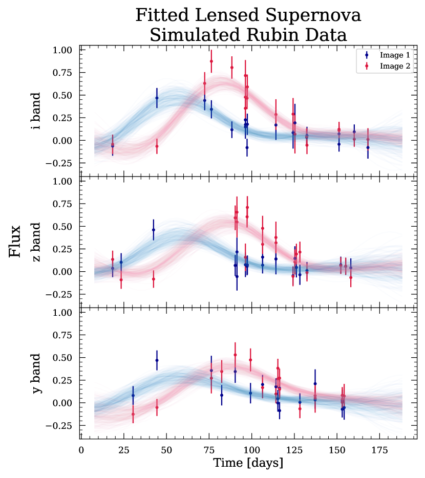
In Figure 6, we show the joint posteriors for the four fitted parameters from the constant magnification fit in a corner plot. GausSN estimates days, a 12.61% precision estimate, and . Although modeling this object is simpler than modeling the Roman objects, for example, because it is not subject to microlensing effects, the sparsity of the data clearly provides a challenge to the model. Even so, the time delay and magnification are still accurately recovered by GausSN.
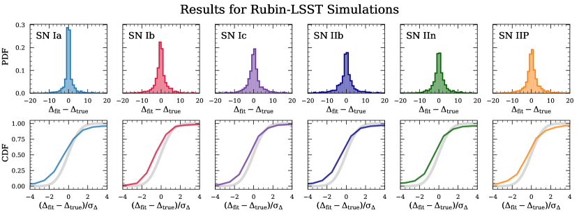
On a population level, GausSN shows effectivenesss in recovering a time delay that is close in absolute value to the true time delay. In the top row of Figure 7, we show the distribution of by subclass of SN. GausSN retrieves 40.67% of time delays within day of the truth, 69.15% within days, and 79.89% within days. We also find that 40.66% of systems have fractional errors of less than 5%. Therefore, regardless of the value of the time delay, the GausSN time-delay estimate is consistently close to the truth.
In addition, the uncertainties on the time delays are well-calibrated, as shown in the CDF of in the bottom row of Figure 7. The fraction of SNe for which the true time delay is captured within the 68% and 95% CI, calculated from the and percentiles of the posterior samples, is 52.01% and 80.60%, respectively. We report these results broken down by subclass of SN in Table 2.
| SN Type | N | < 1 day | < 3 days | < 5 days | < 5% | in 68% CIa | in 95% CIa |
|---|---|---|---|---|---|---|---|
| Ia | 1452 | 0.559 | 0.749 | 0.813 | 0.529 | 0.477 | 0.765 |
| Ib | 1473 | 0.422 | 0.731 | 0.842 | 0.432 | 0.573 | 0.876 |
| Ic | 1416 | 0.369 | 0.693 | 0.812 | 0.385 | 0.55 | 0.835 |
| IIb | 1509 | 0.355 | 0.624 | 0.74 | 0.355 | 0.496 | 0.801 |
| IIn | 1705 | 0.366 | 0.668 | 0.778 | 0.356 | 0.522 | 0.796 |
| IIP | 1717 | 0.369 | 0.685 | 0.808 | 0.383 | 0.503 | 0.763 |
-
a
The fraction of SNe for which falls within the 68% and 95% credible intervals (CI) computed from the and percentiles of the posterior samples.
Only 5.73% of glSNe have fitted time delays which are more than 5 away from the true value. Based on visual inspection of the fits, it is very easy to tell when there has been a catastrophic failure with GausSN for the Rubin-LSST simulations. For the majority of these objects, the posteriors show that the nested sampling chains have run up against the prior bounds, either for the GP length scale or the time delay, suggesting that the prior was not well-chosen for the data. Real glSNe will not be fit in bulk, as the simulated objects are for this analysis, so again more informative priors can be selected for objects on an individual basis to mitigate many of these extreme outliers. Indeed, fitting a few of these objects with more informative priors enabled more accurate time-delay recovery. Therefore, these outliers are not of great concern, as they could be easily flagged and refit with more informative priors to get reliable time-delay estimates.
As with the Roman simulations, there are also several outliers with multi-modal posteriors for which the mean and standard deviation of the samples are simply a poor summary of the posterior. Again, fitting with more informative priors easily solves this problem. Furthermore, we re-emphasize that the full posterior should be used in the cosmological analysis of any glSN. These types of outliers are, therefore, expected and not as concerning.
The results in Table 2 are roughly consistent with those reported for the Roman simulations. However, the mean uncertainty on the time-delay estimate from GausSN on the Rubin-LSST simulations is 7.53 days, highlighting that relative to the Roman simulations, the time-delay estimates for the Rubin-LSST simulations are more uncertain in general. Given that GausSN is a data driven approach, and the Rubin-LSST data is more sparse than the Roman data, this increase in uncertainty is expected. Most importantly, the uncertainties remain equally well-calibrated across two very different sets of data.
Finally, we re-emphasize that these simulations are simplified compared to the real data we expect to collect with Rubin-LSST, as they do not have a realistic distribution of time delays nor do they include the effects of dust extinction or microlensing. The simulations enable a test of GausSN on sparsely sampled data in more than two bands, but the results overestimate the fraction of real glSNe that will have time delays estimated to a given precision using only Rubin-LSST data. That only some of the glSNe discovered with Rubin-LSST will be resolved will additionally reduce this fraction. Therefore, follow-up data is very likely to be necessary to obtain time-delay estimates from glSNe discovered by Rubin-LSST to the level of precision and accuracy presented in this analysis.
6 Application to SN Refsdal
We apply GausSN to the five images of SN Refsdal to demonstrate the model’s performance on real data, as well as on an object with more than two images. Following the publication of Kelly et al. (2023a) and Kelly et al. (2023b), the data was made public444Available at https://dx.doi.org/10.3847/1538-4357/ac4ccb.. The five images of SN Refsdal, images S2-S4 and SX, were observed by the Hubble Space Telescope (HST) in three filters – F105W, F125W, and F160W. As the data in the F105W filter is limited and of worse quality relative to the other two bands, we follow Kelly et al. (2023b) and exclude this data from the time-delay fit.
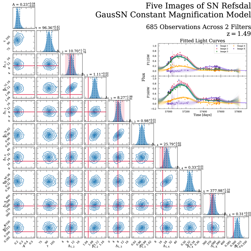
We first fit SN Refsdal with the constant magnification model. The corner plot for the fit is shown in Figure 8. We measure the time delay of the fifth image, SX, which is the most cosmologically interesting due to its long time delay, to be days – a 1.35% precision measurement. In addition, our results are in very good agreement with those reported by Kelly et al. (2023b) for all five images. As shown in Figure 8, the time-delay estimates from GausSN fall within the and percentiles of the posterior distributions on these parameters given in Kelly et al. (2023b). The fitted light curves are shown inset in Figure 8.
As noted in Kelly et al. (2023b), there is evidence for microlensing affecting the light curves, particularly those of images S2, S4, and SX. Therefore, we additionally fit SN Refsdal with the sigmoid magnification function. With the sigmoid magnification function, the time delay for SX, days, is still highly consistent with the previous results. There is only a slight reduction in the precision, with the time delay now measured to 1.43% precision. The time delay of image S3 is also still in very good agreement with Kelly et al. (2023b).
For images S2 and S4, the results are more discrepant from those in the constant magnification fit to the data. With the sigmoid magnification model, GausSN estimates days and days. On the other hand, Kelly et al. (2023b) reports days and days. We emphasize, though, that the results from the individual methods used in the original analysis show additional dispersion in their time-delay estimates that is not well-represented in the values reported above. Therefore, the discrepancy seen in the Kelly et al. (2023b) time-delay estimates and the time-delay estimates reported from the sigmoid magnification model fit in this analysis is not unexpected or of great concern. Most importantly, the results for image SX remain consistent.
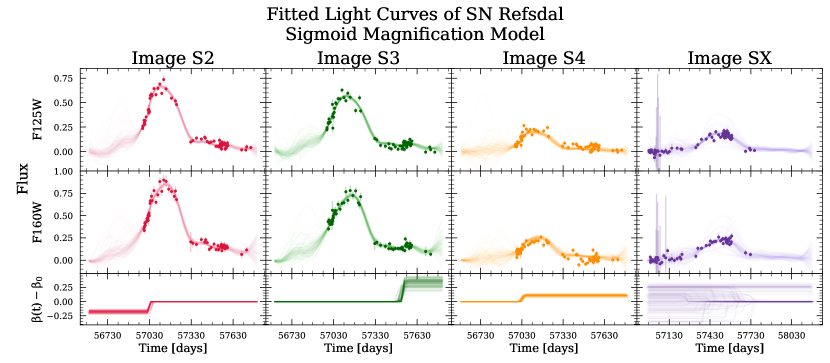
We show realizations of the sigmoid magnification function using draws from the posteriors, as shown in Figure 9. As in Kelly et al. (2023b), we find considerable uncertainty about the effect of microlensing on image SX. There appears to be evidence for microlensing affecting each of images S2-S4, as well. At early times, there is uncertainty in the relative magnification because of the lack of overlapping data from multiple images. However, even around peak, where there is data from other images, the microlensing effect is uncertain. For image S3, the microlensing effect switches on in the tail, where the light curve appears to begin rising again. As this behavior is not seen in the tails of image S2 or S4, it is attributed to microlensing. The magnification from microlensing does not change the shape of the light curve around peak, so it has a minimal effect on the time delay.
Images S2 and S4 show signs of microlensing affecting the beginnings of the light curves. This behavior suggests that images S2 and S4 may exhibit a faster rise than the other images. Interestingly, the time delays of these two images are more discrepant with the Kelly et al. (2023b) results. The rise of the light curves is well-observed for all five images, so we expect that a considerable amount of time-delay constraining power comes from this region of the light curves. Therefore, microlensing affecting images S2 and S4 in this time frame may result in the more significant shift in the time delay from the constant magnification model to the sigmoid magnification model. There is clearly uncertainty in the time-delay fit due to microlensing effects on the light curves, highlighting the importance of accounting for microlensing alongside the time-delay estimate.
7 Discussion
There now exist several methods for extracting time delays from lensed quasars and glSNe. A range of time-delay estimation methods have been used in analyses of lensed quasars. A number of optimization schemes have been paired with spline and GP models of the underlying light curve shape, due to the stochastic nature of the quasar light curves. Among these methods is the widely popular spline-based method PyCS, which was used in the H0LiCOW 2.4% precision estimate (Wong et al., 2020) and adapted for use on SN Refsdal (Kelly et al., 2023b). On the other hand, template-based approaches, such as sntd, have been favored in recent analyses of glSNe (Pierel et al., 2023; Kelly et al., 2023b). We consider below a few advantages to the GausSN approach, which motivate its use alongside other methods in analyses of glSNe discovered in the future, as well as point out where improvements on GausSN can be made.
7.1 Template Choice Uncertainty
SNe are known to have some level of intrinsic variation within each subclass and a number of methods have been used to extract templates from SN light curves. As a result, there are several templates available for each SN subclass which one may chose to fit with using a template-based approach for time-delay estimation. However, the effect of fitting for a time delay with an incorrectly chosen template has yet to be explored. This unknown systematic contributes unaccounted for uncertainties to the time-delay estimate, which may be difficult to propagate through to the uncertainty in a motivated way.
Furthermore, lensing enables us to probe SNe at higher redshifts than would otherwise be observable by existing telescopes. The redshift evolution of SNe is an open question in the field, with an unaccounted for evolution potentially contributing to systematics in cosmological analyses (Nicolas et al., 2021). Therefore, the use of templates based on SNe light curves in the nearby universe similarly introduces a potential source of unaccounted for systematic uncertainty in the time-delay estimate. Especially because templates tend to be based on data from very-nearby SNe to ensure it is high quality, the extremity of this difference will be at its peak for glSNe expected to be discovered by Rubin-LSST, up to , and by Roman, up to .
Being completely independent of templates, GausSN is not subject to this systematic and therefore provides complete Bayesian uncertainties on time-delay estimates without further post-processing to account for such an uncertainty. Given glSNe are attractive for having minimal systematics relative to the distance ladder, keeping sources of systematics to a minimum is important in these analyses.
Finally, if the SN light curve shape is peculiar or without a good template, as was the case with SN Refsdal, template-based approaches must turn to generic templates, such as the Bazin function (Bazin et al., 2009; Karpenka et al., 2013; Villar et al., 2019). The flexibility of generic SN templates can make fitting the templates to the data tedious and sensitive to fine tuning. Alternatively, a custom template may be created for the system. While this approach was possible for SN Refsdal (Kelly et al., 2023b), it will not be feasible in the future as larger numbers of glSNe are discovered. Furthermore, it is difficult to validate an analysis which is based off a custom-made template. GausSN is capable of fitting any object, regardless of its spectroscopic classification, without constructing or fine-tuning a template for the data beforehand.
7.2 Microlensing
Another advantage to GausSN is the treatment of microlensing. The wide ranging nature of the effect which microlensing from stars and substructure can have on a light curve is extremely difficult to constrain (Pierel et al., 2023). For this reason, existing time-delay techniques consider only an additional uncertainty due to microlensing rather than treating it alongside the time-delay estimate. By treating macro- and micro-lensing together as one time-varying magnification term, GausSN marginalizes over only the relative magnification realizations which are consistent with the data. Therefore, the uncertainties from microlensing are propagated through the measurement in a fully Bayesian way and in one step.
We adopt the sigmoid magnification model because it resembles the microlensing curves shown in Foxley-Marrable et al. (2018) and Pierel et al. (2023) and is a convenient fitting function which can be interpreted in a qualitative sense. However, this parametric form is not directly derived from physical models of the microlensing of an expanding photosphere. Furthermore, this treatment does not take advantage of the knowledge of the microlensing magnification distribution. As the photosphere expands, the microlensing effect tends to become less strong because the microcaustics are being averaged over a larger area. Additional parametric models which take advantage of this information can and should be tested within the GausSN framework.
It would also be possible to implement a more flexible and expressive non-parametric microlensing representation within GausSN. Other time-delay estimation methods have used non-parameteric approaches such as splines (Tewes et al., 2013) or simulations from a Gaussian process (Pierel & Rodney, 2019) to quantify the effect of microlensing. Within GausSN such a representation could be implemented seamlessly into the Bayesian model. A natural kernel choice in a GP representation of microlensing could be the non-stationary Gibbs (1997) kernel (see Revsbech et al., 2018, for an example). This would allow for microlensing functions with a short burst of fast magnification change (corresponding to the moment of caustic crossing) and a tendency towards something flatter away from this.
In future work, we intend to explore different parametric and non-parametric magnification models. The comparison of magnification treatments with Bayesian evidence is possible in the nested sampling framework already implemented in the GausSN code.
7.3 Fully Bayesian Treatment
The GausSN framework provides a fully Bayesian treatment of time-delay estimation, but this is just one component of the estimate. A model of the gravitational potential of the lens is necessary to estimate a time-delay distance, which can be used to constain (see e.g. Treu et al., 2022; Suyu et al., 2023). Of course, the time delay and lensing potential are intrinsically linked, meaning there is shared information between these two methods that is not taken advantage of by considering them separately. In the future, a fully Bayesian estimate of the time-delay distance from a combined lens modeling and time-delay estimation method would provide the tightest possible constraints on an estimate.
The most outstanding progress in that direction thus far in the field came from Birrer et al. (2020), which used a hierarchical Bayesian model to jointly infer and galaxy density profiles. GausSN represents a step towards this goal, as well. The GausSN posteriors over the time delay and time-varying magnification parameters could be incorporated into a larger hierarchical Bayesian model for to best utilize all the information available.
8 Conclusion
We have demonstrated that precise and reliable time-delay estimates can be obtained for resolved glSN systems using GausSN, a Bayesian semi-parametric Gaussian Process model. This approach has a number of complementary attributes to existing approaches. In particular, GausSN:
-
•
easily fits glSNe of any type, regardless of whether it has a well-understood light curve shape, without fine-tuning or redshift information,
-
•
is not sensitive to systematic effects introduced by template selection, such as a potential redshift evolution of SNe light curves or fitting with a template that is not representative of the true underlying light curve shape,
-
•
accounts for microlensing alongside time-delay fitting with a modular implementation, which enables any number of microlensing models to be used,
-
•
provides fully Bayesian uncertainties for time-delay estimates without post-processing to account for effects such as microlensing.
GausSN has proven successful on simulations of glSNe as expected from Rubin-LSST and Roman. The Roman simulations from P21 are highly realistic, with careful treatment of survey cadence and depth, dust extinction, and microlensing. Without assuming that the SN type is known and a valid template is available, and without knowledge of the redshift, GausSN maintains a similar performance to the template-based approach sntd. While the results from sntd are based on the assumption of the correct SN-type, template and redshift, GausSN is entirely agnostic to this information. Furthermore, these simulations were not generated from the GausSN forward model, so our results demonstrate the ability of GausSN to generalize.
The simplified Rubin-LSST simulations, created for this analysis using templates from sncosmo, emulate the cadence and depth of the survey. While these simulations do not take into account effects such as dust extinction and microlensing, they test GausSN’s performance on sparsely sampled data. GausSN is successful in predicting time delays which are very close to the true time delay, but the uncertainties on the fits are underestimated in the case of some catastrophic failures. Given the current and projected rates of discovery of glSNe, we expect to have the capacity to inspect the fits individually and choose object-specific priors, which we expect will mitigate any highly inaccurate outliers.
We finally demonstrate the performance of GausSN on the five images of SN Refsdal. Using GausSN, we find that the time delay of image SX is highly consistent with the results from Kelly et al. (2023b), regardless of whether a constant or sigmoid magnification model is used. The time delays of images S2-S4 show more dispersion around the values estimated in Kelly et al. (2023b), but not so much to be concerning, especially given the lessened cosmological interest in these images. As in the original analysis, there is considerable uncertainty in the effect of microlensing on image SX. However, even with the uncertainty due to microlensing accounted for, we are still able to estimate the time delay to 1.43% precision – a level of precision competitive with the estimates reported in Kelly et al. (2023b). GausSN, by fitting for the time delay alongside a time-varying magnification term using the data from all five images simultaneously, provides competitive time-delay constraints using real glSN data, without compromising on fit quality.
There remain many possibilities for extensions of this work to address i) restrictions on the kernel which reflect known physical characteristics of the system, such as constraining the kernel to positive flux only, ii) a test of additional treatments of microlensing, which ideally would be based on physically-interpretable parameters, iii) the incorporation of additional spectroscopic or unresolved light curve information, iv) a treatment of the covariance between light curve shapes in different bands, as we know photometric data to be slices of a continuous SED in time- and wavelength- space, v) incorporation of dust effects from the host and lens into the model, and vi) development of quantitative model checking approaches to assess the reliability of time-delay estimates. We leave addressing these issues to future work.
A percent-level measurement will require more than precise and accurate time-delay estimation. Optimistically, even if Rubin-LSST and Roman on their own provide the necessary photometric data for time day estimation measurements, additional data will be needed from other instruments to enable the complex lens modeling required for an measurement. Fast and synergistic follow-up of glSNe from a variety of instruments will be needed to complete the full cosmological analysis of these objects.
Despite these challenges, the recent increase in the rate of discovery of glSNe and first measurement of from SN Refsdal suggests promise for this young technique. A measurement of to percent level precision from glSNe would be an important new piece of evidence for efforts to determine whether the Hubble tension is driven by systematics or new physics. With upcoming instruments, such as Rubin-LSST and Roman, and precise statistical analysis tools for time-delay extraction, such as GausSN, glSNe show promise to reach this benchmark in the coming decade.
Acknowledgements
We thank Vidhi Lalchand, Sam Ward, and Ben Boyd for useful discussions.
Supernova and astrostatistics research at Cambridge University is supported by the European Union’s Horizon 2020 research and innovation programme under European Research Council Grant Agreement No 101002652 and Marie Skłodowska-Curie Grant Agreement No 873089. ST was supported by the European Research Council (ERC) under the European Union’s Horizon 2020 research and innovation programme (grant agreement no. 101018897 CosmicExplorer). EEH is supported by a Gates Cambridge Scholarship (#OPP1144). NA is supported by the research project grant ‘Understanding the Dynamic Universe’ funded by the Knut and Alice Wallenberg Foundation under Dnr KAW 2018.0067.
Data Availability
The simulated Roman data from Pierel et al. (2021) are publicly available in the MAST Archive at https://dx.doi.org/10.17909/t9-k8w7-zk32. The SN Refsdal data from Kelly et al. (2023b) are publicly available from The Astrophysical Journal at https://dx.doi.org/10.3847/1538-4357/ac4ccb. The simulated Rubin-LSST data are available upon request to the corresponding author.
References
- Baklanov et al. (2021) Baklanov P., Lyskova N., Blinnikov S., Nomoto K., 2021, ApJ, 907, 35
- Barbary et al. (2023) Barbary K., et al., 2023, SNCosmo, Zenodo, doi:10.5281/zenodo.592747
- Bazin et al. (2009) Bazin G., et al., 2009, A&A, 499, 653
- Birrer et al. (2020) Birrer S., et al., 2020, A&A, 643, A165
- Birrer et al. (2022) Birrer S., Dhawan S., Shajib A. J., 2022, ApJ, 924, 2
- Biswas et al. (2019) Biswas R., Setzer C., Azfar F., 2019, LSSTDESC/OpSimSummary: 2.0.0, Zenodo, doi:10.5281/zenodo.2671955
- Biswas et al. (2020) Biswas R., Daniel S. F., Hložek R., Kim A. G., Yoachim P., LSST Dark Energy Science Collaboration 2020, ApJS, 247, 60
- Bonvin et al. (2017) Bonvin V., et al., 2017, MNRAS, 465, 4914
- Bonvin et al. (2018) Bonvin V., et al., 2018, A&A, 616, A183
- Bonvin et al. (2019a) Bonvin V., Tihhonova O., Millon M., Chan J. H. H., Savary E., Huber S., Courbin F., 2019a, A&A, 621, A55
- Bonvin et al. (2019b) Bonvin V., et al., 2019b, A&A, 629, A97
- Boone (2019) Boone K., 2019, AJ, 158, 257
- Chen et al. (2022) Chen W., et al., 2022, Nature, 611, 256
- Chornock et al. (2013) Chornock R., et al., 2013, ApJ, 767, 162
- Craig et al. (2021) Craig P., O’Connor K., Chakrabarti S., Rodney S. A., Pierel J. R., McCully C., Perez-Fournon I., 2021, preprint, (arXiv:2111.01680)
- Delgado et al. (2014) Delgado F., Saha A., Chandrasekharan S., Cook K., Petry C., Ridgway S., 2014, in Angeli G. Z., Dierickx P., eds, Proceedings Volume 9150 Vol. 9150, Modeling, Systems Engineering, and Project Management for Astronomy VI. SPIE, p. 915015, doi:10.1117/12.2056898, https://doi.org/10.1117/12.2056898
- Di Valentino et al. (2021) Di Valentino E., et al., 2021, Classical and Quantum Gravity, 38, 153001
- Diego et al. (2016) Diego J. M., et al., 2016, MNRAS, 456, 356
- Falco et al. (1985) Falco E. E., Gorenstein M. V., Shapiro I. I., 1985, ApJ, 289, L1
- Feroz et al. (2009) Feroz F., Hobson M. P., Bridges M., 2009, MNRAS, 398, 1601
- Foreman-Mackey et al. (2013) Foreman-Mackey D., Hogg D. W., Lang D., Goodman J., 2013, PASP, 125, 306
- Foxley-Marrable et al. (2018) Foxley-Marrable M., Collett T. E., Vernardos G., Goldstein D. A., Bacon D., 2018, MNRAS, 478, 5081
- Frye et al. (2023a) Frye B. L., et al., 2023a, preprint, (arXiv:2309.07326)
- Frye et al. (2023b) Frye B., et al., 2023b, Transient Name Server AstroNote, 96, 1
- Gibbs (1997) Gibbs M. N., 1997, PhD thesis, Cambridge University
- Goldstein et al. (2018) Goldstein D. A., Nugent P. E., Kasen D. N., Collett T. E., 2018, ApJ, 855, 22
- Goldstein et al. (2019) Goldstein D. A., Nugent P. E., Goobar A., 2019, ApJS, 243, 6
- Goobar et al. (2017) Goobar A., et al., 2017, Science, 356, 291
- Goobar et al. (2023a) Goobar A., et al., 2023a, Nature Astronomy, 7, 1098
- Goobar et al. (2023b) Goobar A., et al., 2023b, Nature Astronomy, 7, 1137
- Goodman & Weare (2010) Goodman J., Weare J., 2010, Communications in Applied Math. and Comput. Sci., 5, 65
- Grayling et al. (2023) Grayling M., et al., 2023, MNRAS, 520, 684
- Grillo et al. (2016) Grillo C., et al., 2016, ApJ, 822, 78
- Handley et al. (2015a) Handley W. J., Hobson M. P., Lasenby A. N., 2015a, MNRAS, 450, L61
- Handley et al. (2015b) Handley W. J., Hobson M. P., Lasenby A. N., 2015b, MNRAS, 453, 4384
- Hojjati & Linder (2014) Hojjati A., Linder E. V., 2014, Phys. Rev. D, 90, 123501
- Hojjati et al. (2013) Hojjati A., Kim A. G., Linder E. V., 2013, Phys. Rev. D, 87, 123512
- Hounsell et al. (2018) Hounsell R., et al., 2018, ApJ, 867, 23
- Hsiao et al. (2007) Hsiao E. Y., Conley A., Howell D. A., Sullivan M., Pritchet C. J., Carlberg R. G., Nugent P. E., Phillips M. M., 2007, ApJ, 663, 1187
- Hu & Tak (2020) Hu Z., Tak H., 2020, AJ, 160, 265
- Huber et al. (2019) Huber S., et al., 2019, A&A, 631, A161
- Huber et al. (2021) Huber S., Suyu S. H., Noebauer U. M., Chan J. H. H., Kromer M., Sim S. A., Sluse D., Taubenberger S., 2021, A&A, 646, A110
- Jauzac et al. (2016) Jauzac M., et al., 2016, MNRAS, 457, 2029
- Karamanis & Beutler (2021) Karamanis M., Beutler F., 2021, Statistics & Computing, 31, 61
- Karamanis et al. (2021) Karamanis M., Beutler F., Peacock J. A., 2021, MNRAS, 508, 3589
- Karpenka et al. (2013) Karpenka N. V., Feroz F., Hobson M. P., 2013, MNRAS, 429, 1278
- Kawamata et al. (2016) Kawamata R., Oguri M., Ishigaki M., Shimasaku K., Ouchi M., 2016, ApJ, 819, 114
- Keeton & Kochanek (1997) Keeton C. R., Kochanek C. S., 1997, ApJ, 487, 42
- Kelly et al. (2015) Kelly P. L., et al., 2015, Science, 347, 1123
- Kelly et al. (2016a) Kelly P. L., et al., 2016a, ApJ, 819, L8
- Kelly et al. (2016b) Kelly P. L., et al., 2016b, ApJ, 831, 205
- Kelly et al. (2022) Kelly P., et al., 2022, Transient Name Server Discovery Report, 2022-2356, 1
- Kelly et al. (2023a) Kelly P. L., et al., 2023a, Science, 380, abh1322
- Kelly et al. (2023b) Kelly P. L., et al., 2023b, ApJ, 948, 93
- Kim et al. (2013) Kim A. G., et al., 2013, ApJ, 766, 84
- Meyer et al. (2023) Meyer A. D., van Dyk D. A., Tak H., Siemiginowska A., 2023, ApJ, 950, 37
- Mörtsell & Dhawan (2018) Mörtsell E., Dhawan S., 2018, J. Cosmology Astropart. Phys., 2018, 025
- Naghib et al. (2019) Naghib E., Yoachim P., Vanderbei R. J., Connolly A. J., Jones R. L., 2019, AJ, 157, 151
- Neal (2003) Neal R. M., 2003, Annals of Statistics, 31, 705
- Nicolas et al. (2021) Nicolas N., et al., 2021, A&A, 649, A74
- Oguri (2015) Oguri M., 2015, MNRAS, 449, L86
- Pierel & Rodney (2019) Pierel J. D. R., Rodney S., 2019, ApJ, 876, 107
- Pierel et al. (2018) Pierel J. D. R., et al., 2018, PASP, 130, 114504
- Pierel et al. (2021) Pierel J. D. R., Rodney S., Vernardos G., Oguri M., Kessler R., Anguita T., 2021, ApJ, 908, 190
- Pierel et al. (2023) Pierel J. D. R., et al., 2023, ApJ, 948, 115
- Planck Collaboration et al. (2020) Planck Collaboration et al., 2020, A&A, 641, A6
- Polletta et al. (2023) Polletta M., et al., 2023, A&A, 675, L4
- Qu et al. (2021) Qu H., Sako M., Möller A., Doux C., 2021, AJ, 162, 67
- Quimby et al. (2013) Quimby R. M., et al., 2013, ApJ, 768, L20
- Rasmussen & Williams (2006) Rasmussen C. E., Williams C. K. I., 2006, Gaussian Processes for Machine Learning. MIT Press
- Refsdal (1964) Refsdal S., 1964, MNRAS, 128, 307
- Revsbech et al. (2018) Revsbech E. A., Trotta R., van Dyk D. A., 2018, MNRAS, 473, 3969
- Riess et al. (2022) Riess A. G., et al., 2022, ApJ, 934, L7
- Rodney et al. (2016) Rodney S. A., et al., 2016, ApJ, 820, 50
- Rodney et al. (2021) Rodney S. A., Brammer G. B., Pierel J. D. R., Richard J., Toft S., O’Connor K. F., Akhshik M., Whitaker K. E., 2021, Nature Astronomy, 5, 1118
- Rubin Observatory Survey Cadence Optimization Committee (2023) Rubin Observatory Survey Cadence Optimization Committee 2023, Survey Cadence Optimization Committee’s Phase 2 Recommendations, https://pstn-055.lsst.io/
- Sharon & Johnson (2015) Sharon K., Johnson T. L., 2015, ApJ, 800, L26
- Skilling (2004) Skilling J., 2004, in Fischer R., Preuss R., Toussaint U. V., eds, American Institute of Physics Conference Series Vol. 735, Bayesian Inference and Maximum Entropy Methods in Science and Engineering: 24th International Workshop on Bayesian Inference and Maximum Entropy Methods in Science and Engineering. pp 395–405, doi:10.1063/1.1835238
- Skilling (2006) Skilling J., 2006, Bayesian Analysis, 1, 833
- Speagle (2020) Speagle J. S., 2020, MNRAS, 493, 3132
- Suyu et al. (2023) Suyu S. H., Goobar A., Collett T., More A., Vernardos G., 2023, preprint, (arXiv:2301.07729)
- Tak et al. (2017) Tak H., Mandel K., van Dyk D. A., Kashyap V. L., Meng X.-L., Siemiginowska A., 2017, Annals of Applied Statistics, 11, 1309
- Tewes et al. (2013) Tewes M., Courbin F., Meylan G., 2013, A&A, 553, A120
- Treu et al. (2016) Treu T., et al., 2016, ApJ, 817, 60
- Treu et al. (2022) Treu T., Suyu S. H., Marshall P. J., 2022, A&ARv, 30, 8
- Villar et al. (2019) Villar V. A., et al., 2019, ApJ, 884, 83
- Vincenzi et al. (2019) Vincenzi M., Sullivan M., Firth R. E., Gutiérrez C. P., Frohmaier C., Smith M., Angus C., Nichol R. C., 2019, MNRAS, 489, 5802
- Wojtak et al. (2019) Wojtak R., Hjorth J., Gall C., 2019, MNRAS, 487, 3342
- Wong et al. (2020) Wong K. C., et al., 2020, MNRAS, 498, 1420
- Woosley et al. (1988) Woosley S. E., Pinto P. A., Ensman L., 1988, ApJ, 324, 466
Appendix A The Microlensing Time Delay
To further motivate the inclusion of a time-varying magnification model at the level of time-delay fitting, we demonstrate the error that an additional “microlensing time-delay” can introduce into the time-delay estimate when fitting with a constant magnification model in an example with a known, time-varying magnification term acting on the second image. We sample the light curves of a doubly-imaged SN Ia at , shown in Figure 1, with a two day cadence in Rubin-LSST’s filters. These images are coincident, with , , , , and . We assume a standard deviation on the error of 5% of the measured flux. The “observed” data from the doubly-imaged system is shown in Figure 10.
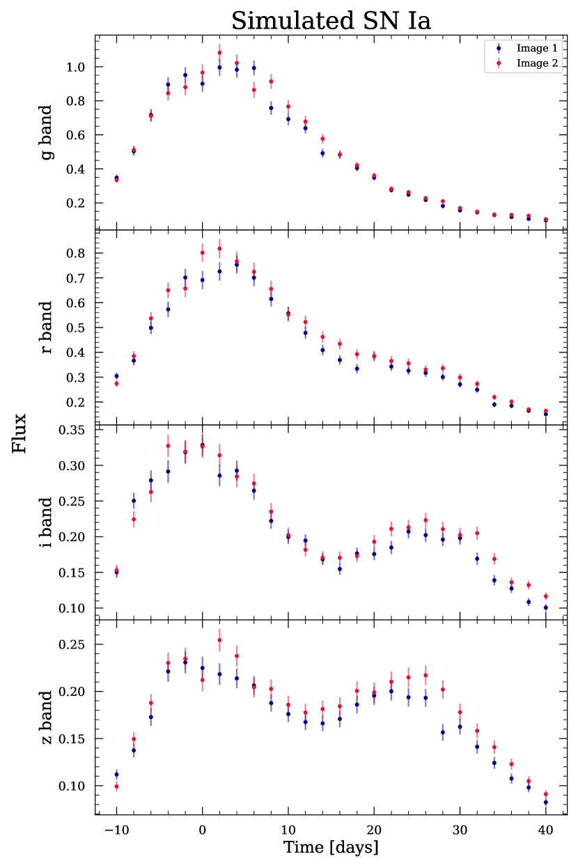
We first fit the object with the constant magnification model with priors on the parameters of:
| (47) | |||
| (48) | |||
| (49) | |||
| (50) |
Figure 11 shows the joint posteriors for the fit. The time delay, , is overestimated at 4 significance. The magnification is estimated to be , which is approximately the mean of the magnification term. This result shows how the model must compromise the time-delay fit because it lacks flexibility. Therefore, a time-varying magnification source can be a significance source of bias if not accounted for in one’s time-delay estimation method.
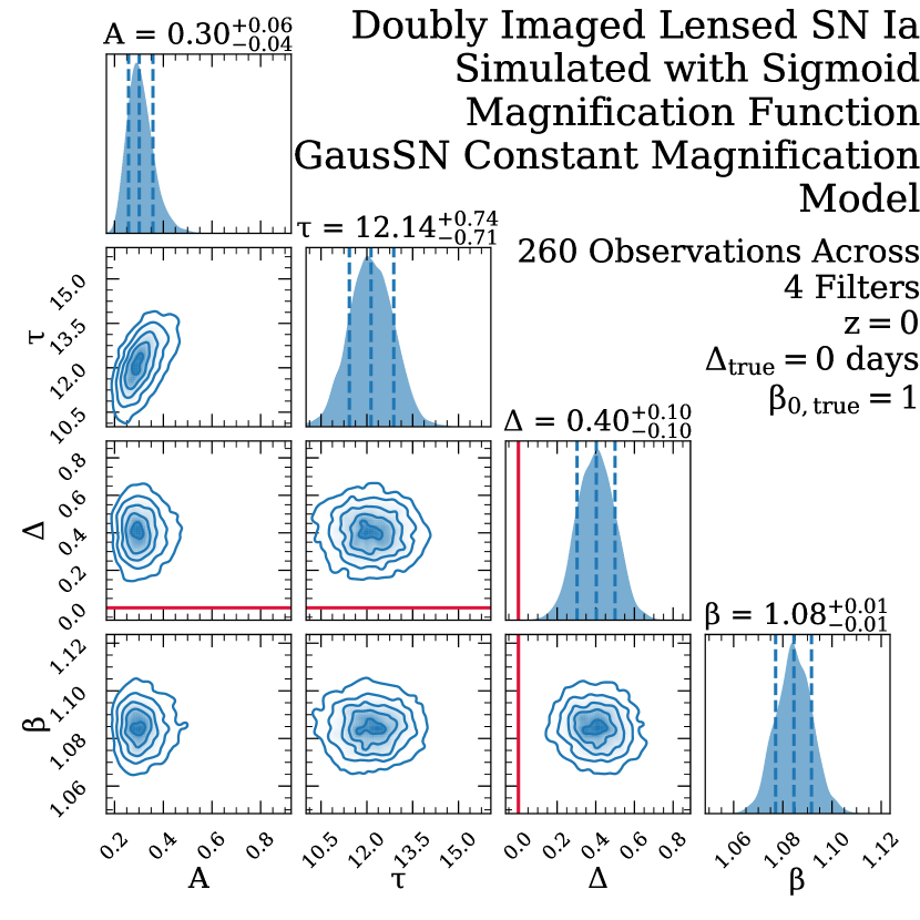
We then fit this example system with the sigmoid magnification model to see if there is an improvement in the quality of fit when allowing a more flexible magnification treatment. We use the same priors as above, as well as the following priors for the additional magnification parameters:
| (51) | |||
| (52) | |||
| (53) |
The joint posteriors for this fit are shown in Figure 12. The time delay is estimated to be , which is both closer to the truth than the constant magnification fit and captures the truth within the confidence interval. The estimated uncertainties are larger, but this more appropriately reflects our level of uncertainty due to the difficulty of constraining time-varying magnification from the light curves of the images alone.
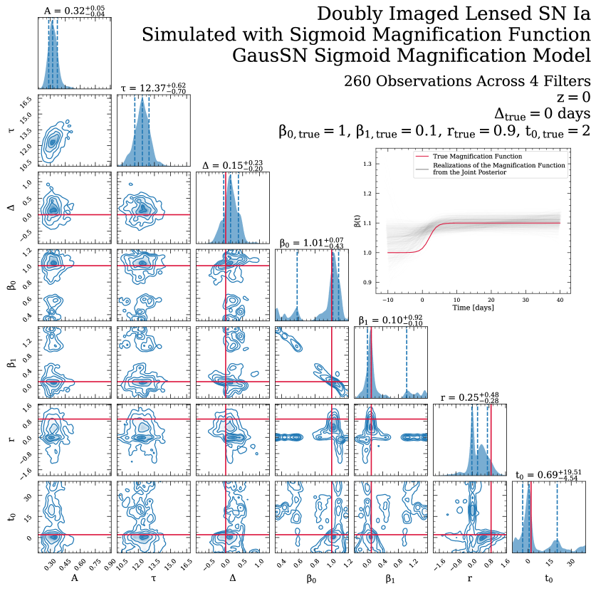
Furthermore, we can use this example to check that the magnification curve is well-recovered by GausSN. The inset plot in Figure 12 shows 1,000 realizations of the magnification function based on draws from the posterior distribution of the sigmoid magnification fit to the data. The true magnification function, over-plotted in the figure, is consistent with the fitted magnification curves, demonstrating qualitatively the ability of GausSN to recover the true underlying relative magnification.