Bounding the Dimension-5 Seesaw Portal with Non-Pointing Photon Searches

Abstract

The addition of $d=5$ operators to the Seesaw model leads to the Dimension-5 Seesaw Portal. Here, two new operators provide interactions for the heavy sterile neutrinos. In particular, the Higgs boson can have a large branching ratio into two heavy neutrinos, meaning that these states can be searched for at the LHC. Moreover, the heavy neutrinos can now decay dominantly into light neutrinos and photons. If the heavy neutrinos are long-lived, then searches for delayed, non-pointing photons can constrain the model. In this work, we carry out a detailed recast of an ATLAS search for such displaced photons, triggered by a charged lepton produced in association to the Higgs, placing bounds on the branching ratio for Higgs decay into two heavy neutrinos as low as $2\%$.

I Introduction

The Standard Model can be extended with sterile neutrinos $\nu_{Rs}$ in order to account for the light neutrino mass pattern measured in oscillation experiments. The simplest model providing also an explanation of the mass hierarchy between the observed light neutrino states $\nu_{\ell}$ and the other fermion masses, generated only by the Yukawa interactions, is the Seesaw mechanism [1, 2, 3, 4, 5]. In its simplest versions, it is enough to include two sterile states, which have a Yukawa interaction with SM leptons as well as a Majorana mass term, to obtain a realistic phenomenology. The diagonalization of the mass terms gives the light neutrino states $\nu_{\ell}$, as well as heavier states $N_{h}$ that interact with the SM particles via their mixing with the active left-handed states.

The Seesaw is on its own a renormalizable UV complete theory, in the same sense as the SM is. However, when considering right-handed neutrinos at the electroweak scale, one can take it as a low energy effective field theory (EFT), extended with higher dimensional effective operators built from the SM and the right-handed neutrino fields. This theory is currently known as $\nu_{R}$SMEFT, with a Lagrangian written as:

$$\mathcal{L}=\mathcal{L}_{SM}+\mathcal{L}_{Seesaw}+\sum_{d>4}\frac{\alpha_{\mathcal{J}}}{\Lambda^{d}}\,\mathcal{O}^{d}_{\mathcal{J}}+h.c.~{},$$ (1)

where the operators $\mathcal{O}_{\mathcal{J}}$ are Lorentz and gauge invariant, and $\Lambda$ is the new physics scale. This EFT, with operators known up to dimension $d=9$ [6, 7, 8, 9, 10], leads to a very rich phenomenology, which has been thoroughly studied in the recent years [11, 12, 13, 14, 15, 16, 17, 18, 19, 20, 21, 22, 23, 24, 25, 26, 27, 28, 29, 30, 31, 32, 33, 34, 35, 36, 37, 38, 39, 40, 41, 42, 43, 44, 45, 46]. Even though the new interactions are suppressed by the scale $\Lambda$, it is well known that the Seesaw mixing is strongly constrained [47, 48, 49]. Thus, it is reasonable to expect that the interactions coming from $\mathcal{O}_{\mathcal{J}}$ can be comparable, if not more important, than those coming from the Seesaw.

In this work we focus on the Dimension-5 Seesaw Portal, that is, the Seesaw model extended with $d=5$ effective operators $\mathcal{O}_{N\phi}$ and $\mathcal{O}_{NB}$. The new interactions provide, in particular, a new pair-production mode from an exotic decay of the Higgs boson $H\to N_{h}N_{h^{\prime}}$, and a dipole interaction between the sterile neutrino states and the photon, which are both the subject of our present study.

The neutrino dipole portal $\mathcal{O}_{NB}$ has caught renovated attention since its proposal as an explanation of the LSND and MiniBooNE anomalies [50, 51]. Many recent works explore bounds on the neutrino dipole interactions from the intensity, energy and cosmic frontiers, among them [52, 53, 54, 55, 56]. In particular, in our last work [37] we reviewed existing constraints on the neutrino dipole coupling, and re-evaluated the LEP bounds from $e^{+}e^{-}\to N_{h}\,\nu$ production. We found that the dipole coupling could not be constrained, unless the mixing was enhanced many orders of magnitude above its naive Seesaw value. In addition, future searches with the capacity of probing the dipole portal have been studied recently at future lepton and hadron colliders [57, 58, 59], long-lived particle detectors at the LHC [60, 38] and from meson decays at the HL-LHC [61], as well as at neutrino telescopes [62].

On the other hand, Higgs decay involving heavy Majorana neutrinos was originally calculated in [63]. Attempts to probe it have been carried out for both prompt [64, 65] and long-lived heavy neutrinos [66]. Moreover, the authors in [67] used the LHC Higgs data to derive constraints on electroweak-scale sterile Dirac neutrinos. This decay has also received attention in extended models, again for prompt [68] and long-lived particles [69, 70].

In the context of the Dimension-5 Seesaw Portal, estimations of the LHC sensitivity reach to test the operator $\mathcal{O}_{N\phi}$ are given in [14, 22], where the authors consider $pp\to H\to N_{h}N_{h}$ for different triggers, with the subsequent displaced decay of the heavy neutrinos into $l^{\pm}qq^{\prime}$ via the Seesaw mixing. Morover, in [29], the authors calculate the projected sensitivities of various future Higgs factories to the Seesaw mixings and the branching ratio ${\rm BR}(H\to N_{h}N_{h})$ using similar processes. This sensitivity is also studied at the HL-LHC in [71], with the use of delayed electron signals.

To the best of our knowledge, the combined presence of both operators has not been studied using LHC data in order to place bounds on the model. In this work, we extend our results in [37] and focus on a scenario where the heavy neutrinos are pair-produced via the Higgs portal $\mathcal{O}_{N\phi}$, and can decay to a photon and a light neutrino via the dipole portal $\mathcal{O}_{NB}$. In the regime where the heavy neutrinos $N_{h}$ are long-lived, this leads to final states with photons which are displaced, delayed and non-pointing, a remarkable signal which has been recently searched for at the LHC [72]. By carefully recasting this search in terms of the Dimension-5 Seesaw Portal interactions, bounds are placed, for the first time, on the coefficient of the $\mathcal{O}_{N\phi}$ operator, based on an existing LHC result. These bounds are applicable provided that the dipole interaction strength allows for the $N_{h}$ to be long-lived but still decay inside the detector, disintegrating primarily into final states with photons.

The paper is organised as follows. In Section II, we review the model and present the associated processes that will be critical for the search. In Section III we provide a detailed description of our recast of the search for delayed photons, report our statistical analysis, and show our final results. We finally conclude in Section IV.

II Overview of the Dimension-5 Seesaw Portal

The standard Seesaw model, with two sterile neutrinos $\nu_{R}$, has the following Lagrangian:

$$\mathcal{L}=\mathcal{L}_{SM}+i\bar{\nu}_{Rs}\,\not{\partial}\,\nu_{Rs}-\left(\bar{L}_{a}(Y_{\nu})_{as}\,\tilde{\phi}\,\nu_{Rs}+\frac{1}{2}\bar{\nu}_{Rs}(M_{N})_{ss^{\prime}}\nu^{c}_{Rs^{\prime}}+h.c.\right)~{},$$ (2)

where $a=e,\,\mu,\,\tau$ and $s,s^{\prime}=s_{1},s_{2}$. The $Y_{\nu}$ couplings are connected to Dirac masses, which appear on the neutrino mass matrix alongside the symmetric Majorana mass $M_{N}$. As is well known, after diagonalization two non-zero masses for the SM neutrinos can be obtained. Light states are thus denoted $\nu_{\ell}$ ($\ell=1,\,2,\,3$), with masses $m_{\ell}$, while heavy states are denoted $N_{h}$ ($h=4,\,5$), with masses $M_{h}$. Heavy neutrinos can be probed through their active neutrino component, as parametrized in the mixing matrix $U$, which allows them to interact via the $W$ and $Z$ bosons. The latest bounds on these mixings can be found in [73, 49].

In the following, we extend the Seesaw with the following $d=5$ operators:

$$\mathcal{L}_{5}=\frac{(\alpha_{N\phi})_{ss^{\prime}}}{\Lambda}(\phi^{\dagger}\phi)\,\bar{\nu}_{Rs}\,\nu^{c}_{Rs^{\prime}}+\frac{(\alpha_{NB})_{ss^{\prime}}}{\Lambda}\bar{\nu}_{Rs}\,\sigma^{\mu\nu}\nu^{c}_{Rs^{\prime}}\,B_{\mu\nu}+h.c.~{},$$ (3)

where $\sigma^{\mu\nu}=\tfrac{i}{2}[\gamma^{\mu},\,\gamma^{\nu}]$. These are referred to as Anisimov-Graesser $\mathcal{O}_{N\phi}$ [75, 76, 77] and dipole $\mathcal{O}_{NB}$ [7] operators, respectively. The former involves a symmetric coefficient $\alpha_{N\phi}$, while the latter has an antisymmetric $\alpha_{NB}$. It is important to point out that, although denoted as $\alpha_{N\phi}/\Lambda$ and $\alpha_{NB}/\Lambda$, the new physics scale $\Lambda$ does not necessarily have to be the same.

The inclusion of these operators modifies the neutrino mass matrix, as well as their couplings. Following [37], we will neglect all effects on the masses, and concentrate exclusively on the new interactions. In the following, we list all interaction terms relevant for our work. First, the Anisimov-Graesser operator allows the coupling of the Higgs to two heavy neutrinos:

$$\mathcal{L}_{h}=\frac{v}{\Lambda}H\,\bar{N}_{h}\left[(\alpha^{\prime*}_{N\phi})_{hh^{\prime}}P_{R}+(\alpha^{\prime}_{N\phi})_{hh^{\prime}}P_{L}\right]\,N_{h^{\prime}}~{},$$ (4)

with $(\alpha^{\prime}_{N\phi})_{hh^{\prime}}=U_{sh}\,(\alpha_{N\phi})_{ss^{\prime}}\,U_{s^{\prime}h^{\prime}}$, having $U_{sh}\sim I$ as the “sterile-heavy” mixing sector of $U$. In principle, the Higgs can also couple to two heavy neutrinos through the $Y_{\nu}$ coupling in the standard Seesaw. This, however, is very strongly suppressed, as in addition to the smallness of $Y_{\nu}$, the coupling also requires an “active-heavy” mixing, $U_{ah}\sim\sqrt{m_{\ell}/M_{h}}$.

The dipole operator allows the heavy neutrinos to interact with the photon and $Z$ bosons:

$$\mathcal{L}_{ZNN} = -\frac{s_{W}}{\Lambda}(\partial_{\mu}Z_{\nu}-\partial_{\nu}Z_{\mu})\,\bar{N}_{4}\,\sigma^{\mu\nu}\left[(\alpha^{\prime}_{NB})_{45}P_{L}-(\alpha^{\prime\,*}_{NB})_{45}P_{R}\right]N_{5}+h.c.~{},$$ (5)

$$\mathcal{L}_{\gamma NN} = \frac{c_{W}}{\Lambda}(\partial_{\mu}A_{\nu}-\partial_{\nu}A_{\mu})\,\bar{N}_{4}\,\sigma^{\mu\nu}\left[(\alpha^{\prime}_{NB})_{45}P_{L}-(\alpha^{\prime\,*}_{NB})_{45}P_{R}\right]N_{5}+h.c.~{}.$$ (6)

As in the previous case, we define $(\alpha^{\prime}_{NB})_{45}=U_{s4}\,(\alpha_{NB})_{ss^{\prime}}\,U_{s^{\prime}5}$. Given that the coupling is antisymmetric, the heavy neutrinos involved must necessarily be different. It is worth noting that, similarly to the Higgs, a coupling with the $Z$ is also allowed by the standard Seesaw, but is also heavily suppressed.

Finally, we report the coupling of one heavy neutrino, a light neutrino (or charged lepton) and a gauge boson:

$$\mathcal{L}_{W} = \frac{g}{\sqrt{2}}W_{\mu}^{-}\bar{\ell}_{a}\gamma^{\mu}\,U_{ah}\,P_{L}\,N_{h}+h.c.~{},$$ (7)

$$\mathcal{L}_{Z} = \frac{g}{4c_{W}}Z_{\mu}\bar{\nu}_{\ell}\gamma^{\mu}\,\left(C_{\ell h}\,P_{L}-C_{\ell h}^{*}\,P_{R}\right)\,N_{h}$$ (8)

$$-\frac{s_{W}}{\Lambda}(\partial_{\mu}Z_{\nu}-\partial_{\nu}Z_{\mu})\,\bar{\nu}_{\ell}\,\sigma^{\mu\nu}\left[(\alpha^{\prime}_{NB})_{\ell h}P_{L}-(\alpha^{\prime\,*}_{NB})_{\ell h}P_{R}\right]N_{h}+h.c.~{},$$

$$\mathcal{L}_{\gamma} = \frac{c_{W}}{\Lambda}(\partial_{\mu}A_{\nu}-\partial_{\nu}A_{\mu})\,\bar{\nu}_{\ell}\,\sigma^{\mu\nu}\left[(\alpha^{\prime}_{NB})_{\ell h}P_{L}-(\alpha^{\prime\,*}_{NB})_{\ell h}P_{R}\right]N_{h}+h.c.~{},$$ (9)

with $C_{\ell h}=U^{*}_{a\ell}\,U_{ah}$ and $(\alpha^{\prime}_{NB})_{\ell h}=U_{s\ell}\,(\alpha_{NB})_{ss^{\prime}}\,U_{s^{\prime}h}$. These are always suppressed, either by $U_{ah}$ or by the “sterile-light” mixing, $U_{s\ell}\sim\sqrt{m_{\ell}/M_{h}}$.

II.1 Production and Decay Channels at the LHC

We consider heavy neutrino pair production from Higgs decays. In our model, this decay is dominated by the couplings appearing in Eq. (4). Taking them as real, the corresponding partial width is [76, 7]:

$$\Gamma(H\to N_{h}\,N_{h^{\prime}})=S_{hh^{\prime}}\frac{v^{2}}{2\pi}\frac{\sqrt{\lambda(m_{H}^{2},\,M_{h}^{2},\,M_{h^{\prime}}^{2})}}{m_{H}}\left|\frac{(\alpha^{\prime}_{N\phi})_{hh^{\prime}}}{\Lambda}\right|^{2}\left(1-\frac{(M_{h}+M_{h^{\prime}})^{2}}{m_{H}^{2}}\right)~{}.$$ (10)

Here, $m_{H}$ is the Higgs mass, $\lambda(x,\,y,\,z)=x^{2}+y^{2}+z^{2}-2xy-2xz-2yz$, and $S_{hh^{\prime}}$ provides a factor $1/2$ if the two outgoing heavy neutrinos are the same.

The decay of the Higgs into two $N_{4}$, two $N_{5}$ or an $N_{4}\,N_{5}$ pair depends on the structure of the couplings $\alpha^{\prime}_{N\phi}$. As presented in [14, 37], in order to explain the size difference between the coefficients of the Weinberg operator and both $\mathcal{O}_{N\phi}$ and $\mathcal{O}_{NB}$ operators, one could argue the existence of a slightly broken lepton number symmetry. From this, one would expect the diagonal elements of $\alpha_{N\phi}$ to be very suppressed, meaning that $H\to N_{4}\,N_{5}$ would be favoured. In what follows, we will consider this decay exclusively.

Since we are taking $M_{4}<m_{H}/2$, the lightest heavy neutrino $N_{4}$ will either decay into a light neutrino and a photon, or into a variety of final states described by three-body decays. The $\nu_{\ell}\,\gamma$ decay is mediated by $\alpha_{NB}$, and was first calculated in [7]:

$$\Gamma(N_{4}\to\,\nu\,\gamma)=\frac{2}{\pi}\,c_{W}^{2}M_{4}^{3}\sum_{\ell}\left|\frac{(\alpha^{\prime}_{NB})_{\ell 4}}{\Lambda}\right|^{2}~{},$$ (11)

where $c_{W}$ is the cosine of the weak mixing angle. Since this decay mode requires the heavily suppressed sterile-light mixing, the width is small, allowing for $N_{4}$ to be long-lived.

The calculation of three-body decays are somewhat more complicated, as the mixing with interaction states leads to diagrams with virtual $W^{\pm}$ and $Z$ bosons (see [78, 79, 80, 81, 82] for the corresponding widths in the standard Seesaw). As was shown in [37], it is very important to include three-body decays in order to estimate correctly the heavy neutrino decay length. In addition, it is also possible to introduce new contributions involving a virtual $Z$ or photon, however, these have a very small impact on the branching ratios and decay lengths within the region of the parameter space we are interested in. The full formulae can be found in Appendix B of [37].

If the Higgs decays into two heavy neutrinos of different mass, the heaviest is expected to decay via either $N_{5}\to N_{4}\,\gamma$ or $N_{5}\to N_{4}\,Z$, as their couplings are not suppressed by mixing. For simplicity, in the following we will restrict ourselves to $\Delta M\equiv M_{5}-M_{4}<M_{Z}$, so the latter is forbidden. In this case, the width of the heavy neutrino is given by [7]:

$$\Gamma(N_{5}\to\,N_{4}\,\gamma)=\frac{2}{\pi}\,c_{W}^{2}\frac{(M_{5}^{2}-M_{4}^{2})^{3}}{M^{3}_{5}}\left|\frac{(\alpha^{\prime}_{NB})_{45}}{\Lambda}\right|^{2}~{},$$ (12)

Notice that, compared to Eq. (11), this width depends on $(\alpha^{\prime}_{NB})_{hh^{\prime}}$ instead of $(\alpha^{\prime}_{NB})_{\ell h}$. As mentioned before, this implies that the decay will proceed without the need of sterile-light mixing, so it will not be suppressed. Thus, apart from rendering the $N_{5}$ as short-lived, three body decays are irrelevant when calculating the $N_{5}$ width.

An exception to this expectation might arise if the heavy neutrinos are pseudo-Dirac particles, with practically degenerate masses. As for the dimension-5 operator hierarchy, this possibility can be expected in the presence of an approximate lepton number symmetry [83, 84, 85, 86, 87], which is a feature of several Seesaw realizations [88, 89, 90, 91]. In front of this, decays of $N_{5}$ exclusively into SM particles, such as the one shown in Eq. (11), can dominate if:

$$\left(1-\frac{M^{2}_{4}}{M^{2}_{5}}\right)\ll|U_{s\ell}|^{2}~{}.$$ (13)

For instance, as shown in [92, 93], in certain models the heavy mass splitting could be as low as the light neutrino solar mass splitting, implying that the term on the left-hand side of Eq. (13) would be of order $10^{-14}$, for GeV masses. Thus, if the mixing on the right-hand side was larger than this, it would be necessary to calculate both two and three body decays for $N_{5}$, as is done for $N_{4}$. In this work we will assume that the mass splitting is always large enough such that this never happens. In particular, we assume that the mixing is never above the naive Seesaw expectation, which maximises the lifetime of $N_{4}$.

III Bounds from Non-Pointing Photon Searches

The ATLAS search for non-pointing photons [72] used $\mathcal{L}=139$ fb^-1 of data collected from proton-proton collisions at a center-of-mass energy of $\sqrt{s}=13$ TeV. It is assumed that the photons come from the decays of a pair of LLPs, generated in turn by the decay of the Higgs boson. The measurement is triggered by a prompt electron or muon, with $p_{T}>27$ GeV, coming from associated production with the Higgs.

As in the search, our simulation considered the triggering leptons coming from $p\,p\to W^{\pm}H$, $p\,p\to Z\,H$ and $p\,p\to t\,\bar{t}\,H$ processes. Events were generated with MadGraph5_aMC@NLO 2.9.7 [94], which uses LHAPDF6 [95]. The model was the same of [37], based on FeynRules 2.3.43 [96, 97]. The heavy neutrino decay, parton showering and hadronization was carried out by PYTHIA 8.244 [98], giving a HepMC file as output [99, 100]. The cross-sections, calculated at leading order, were multiplied by appropriate K-factors, following [101].

III.1 Arrival Time and Non-Pointing Parameter

The analysis in [72] relies on two kinematical variables. The first is the time delay $t_{\gamma}$, that is, the difference between the arrival time and that expected from a prompt photon. The second one is the non-pointing parameter $|\Delta z_{\gamma}|$, defined as the distance between the interaction point and the extrapolated trajectory of the reconstructed photon, measured along the beamline. In our work, both $t_{\gamma}$ and $|\Delta z_{\gamma}|$ were calculated for all photons from truth-level information, extracted from the HepMC output of PYTHIA. Our procedure was first outlined in [37], which we reproduce here for the convenience of the reader.

In order to determine $t_{\gamma}$, we calculated the absolute time $t^{\prime}$ for each photon to enter the ECal, which depends on the heavy neutrino momentum $\vec{p}_{N}$, its decay position $\vec{r}_{N}$, and the direction of the photon momentum $\vec{p}_{\gamma}$ after the decay. The region where each photon entered the ECal would be mapped to a specific pseudorapidity $\eta$. Similarly, it is possible to calculate the corresponding time $t_{0}$ related to prompt photons, also as a function of $\eta$. With these two, the time delay is simply $t_{\gamma}=t^{\prime}-t_{0}$.

On the other hand, we calculated $|\Delta z_{\gamma}|$ using (see Appendix C of [102]):

$$|\Delta z_{\gamma}|=\left|\frac{r_{N_{z}}-p_{\gamma_{z}}(\vec{p}_{\gamma}\cdot\vec{r}_{N})/|\vec{p}_{\gamma}|^{2}}{1-p_{\gamma_{z}}^{2}/|\vec{p}_{\gamma}|^{2}}\right|~{},$$ (14)

where we have assumed that the primary vertex lies at the center of the detector. The variables $r_{N_{z}}$ and $p_{\gamma_{z}}$ denote the components of $\vec{r}_{N}$ and $\vec{p}_{\gamma}$ on the $z$-axis.

Once this information was obtained, it was stored within the same HepMC file, and passed on to Delphes in order to carry out the detector simulation.

III.2 Event Reconstruction in Delphes

The event reconstruction is partially simulated by Delphes 3.5.0 [103], which depends on FastJet 3.4.0 [104]. We modified the code, such that it would read the $t_{\gamma}$ and $|\Delta z_{\gamma}|$ information stored within the HepMC file, and later include it in its output.

The detector simulation includes most modules from the ATLAS card packaged within Delphes, with appropriate modifications. To begin with, the ParticlePropagator module was modified in order to give more details of the ATLAS dimensions [105], so, apart from the magnetic field coverage of $1.15\,$m, and a half-length of $3.512\,$m, we also specified an ECal inner radius of $1.5\,$m (RadiusMax$=1.5$).

For photons, we left all calorimetry modules untouched, returning EFlow photons with reconstructed $p^{\gamma}_{T}$. Following [72], we modified the photon track isolation, such that it required the scalar sum of $p_{T}$ of all tracks within $\Delta R=0.2$ of the photon, with $p_{T}>1\,$GeV, to be less than $5\%$ of $p^{\gamma}_{T}$. In addition, we added a photon calorimeter isolation module, which required the sum of all energy deposits on the ECal, within $\Delta R=0.2$, to be less than $6.5\%$ of $p_{T}^{\gamma}$. The photon ID efficiency was set to $100\%$, with the real efficiency to be applied outside of Delphes (see below).

For electron reconstruction we proceeded almost identically as for photons. The electron track isolation restricted the sum of $p_{T}$ of additional tracks around the electron to be less than $15\%$ of the reconstructed electron transverse momentum, $p^{e}_{T}$. The calorimeter isolation would then require other energy deposits to be less than $20\%$ of $p^{e}_{T}$. Finally, the electron ID efficiency was also to be implemented outside Delphes.

For muons, we eliminated the isolation module and set a $100\%$ ID efficiency, with the objective of applying both outside Delphes. For jets, we set the $R$ parameter to $0.4$, and a minimum $p_{T}$ of $25\,$GeV. Finally, we deactivated the UniqueObjectFinder module, as the overlap removal was to be implemented after the ID efficiencies had been applied, based on the specific requirements in [72]. As commented earlier, the Delphes output routines were also modified, such that the $t_{\gamma}$ and $|\Delta z_{\gamma}|$ variables were written for each reconstructed photon.

III.3 Event Selection

As noted above, the event reconstructed in our Delphes implementation is incomplete. In the following, we describe how we finalise the detector simulation, and furthermore give details on the event selection and analysis performed in [72].

The photons selected for the analysis must satisfy basic cuts, such as having $p_{T}>10\,$GeV and $\eta<2.37$ (with the region between the ECal barrel and endcaps excluded), as well as being generated within the Inner Detector, before the ECal. In order to take into account the experimental resolution, both $t_{\gamma}$ and $|\Delta z_{\gamma}|$ variables were each Gaussian smeared. For $|\Delta z_{\gamma}|$, the resolution for the smear was taken from an interpolation of the data shown in Figure 1 of [106]. For $t_{\gamma}$, we interpolated the data in Figure 2 of [72]. The latter Figure is presented as a function of $E_{\rm cell}$, defined as the middle-layer ECal cell receiving the maximum energy deposit of the shower. For definiteness, following the claim in [72] of $E_{\rm cell}$ being around $20$-$50\%$ of the total energy deposited by the shower, we set $E_{\rm cell}=0.35\,p_{T}^{\gamma}$.

Given the smeared value for $|\Delta z_{\gamma}|$, we applied the photon ID efficiency shown in Figure 3 of [72]. Then, following the procedure of the search, at least one photon was required to be in the ECal barrel. Events satisfying this constraint were divided into single or multi-photon channels. In the case of having more than one photon in the barrel, the one with the largest $p_{T}^{\gamma}$ was used for the analysis. For this photon, a further cut $E_{\rm cell}>10\,$GeV was imposed.

Regarding charged leptons, only those with $p_{T}>10\,$GeV would be considered in the analysis. Electrons would be restricted to $\eta<2.47$, again excluding the region between the ECal barrel and endcap, while muons would be required to have $\eta<2.7$. For the electron ID efficiency, we followed the data within both panels in Figure 17 of [107], for medium electrons. Furthermore, for muon isolation and ID efficiency, we followed the total identification efficiency curve in Figure 21 of [108].

Turning to jets, apart from the $p_{T}>25\,$GeV cut outlined above, we also asked for a rapidity $|y|<4.4$. Having defined photons, electrons, muons and jets, we proceeded with the overlap removal in [72]. Thus, all electrons with $\Delta R\leq 0.4$ from a photon were removed from the event. Then, all jets within $\Delta R\leq 0.4$ from a photon, or $\Delta R\leq 0.2$ from an electron, were removed. Next, in order to match the requirements appearing in the measurement of isolated electron efficiencies, all electrons within $\Delta R\leq 0.4$ from the surviving jets were removed. Finally, all muons within $\Delta R\leq 0.4$ from photons or jets were also removed.

With these unique, reconstructed objects in hand, the search required one charged lepton to match the triggering lepton. In other words, one of the surviving electrons or muons must have $p_{T}>27\,$GeV. If the triggering lepton is an electron, then the invariant mass of the electron - photon pair, $m_{e\gamma}$, must also satisfy $|m_{e\gamma}-m_{Z}|>15\,$GeV. With this, the event is selected for analysis.

In order to be assigned to the signal region, the missing transverse energy (MET) must be larger than 50 GeV. Events in the signal region are then classified into five categories, depending on the value of $|\Delta z_{\gamma}|$. Within each category, events are binned following the value of $t_{\gamma}$. The binning depends on whether the event sample is in the single or multi-photon channel.

We have validated our recast by implementing the signal model of [72], and generating the timing distributions for all $|\Delta z_{\gamma}|$ categories, for both channels. The resulting events in each category were consistent in order of magnitude and in behaviour with respect to $t_{\gamma}$, compared to Figure 7 of [72].

III.4 Statistical Analysis

We now turn to the statistical analysis used to constrain our model. We remind the reader that the long-lived heavy neutrinos are produced via $H\to N_{4}\,N_{5}$ decay, which in turn disintegrate into final states with photons. The constraints on the total number of signal events can then be translated as bounds on the Higgs branching ratio into $N_{4}\,N_{5}$, which can then be expressed in terms of $(\alpha^{\prime}_{N\phi})_{45}/\Lambda$ using Equation (10). Our objective is to constrain this parameter as a function of the heavy neutrino mass and lifetime, the latter depending on $\alpha_{NB}/\Lambda$.

To this end, we use the model independent results presented by ATLAS in [72], which focuses on the last timing $t_{\gamma}$ bin of the category with largest non-pointing $|\Delta z_{\gamma}|$, for single and multi-photon channels. The number of measured events in such bins, as well as the backgrounds, are given in Table II of [72]. Specifically, the single (multi-) photon channel uses a $t_{\gamma}$ bin between 1.5 and 12 ns (1 and 12 ns), observing 4 (0) events, while expecting $3.8\pm 1.6$ ($0.28\pm 0.04$). Both channels focus on $|\Delta z_{\gamma}|>300\,$mm. The Table also presents a combination of both channels, with 4 events observed and $4.1\pm 1.7$ expected.

Our 95% exclusion limits are calculated using the CLs method. This method generally overcovers the confidence interval, with the objective of avoiding setting bounds on signal rates which the experiment is insensitive to. This occurs because it takes into account possible background underfluctuations [109], and thus gives softer bounds than the CL method. Our implementation follows the PDG review on Statistics [110] and Apprendix B in [52]. We consider a counting experiment with a Poisson likelihood function, and calculate the upper number of signal events $s^{up}$ consistent at $(1-\alpha)=95\%$ confidence level with the observation of $n$ events and a background prediction of $b$ events. This is done solving for $s^{up}$ in the following equation

$$\alpha^{\prime}=\frac{\alpha}{(1-\alpha_{b})}=0.05~{},$$ (15)

where

$$\alpha=e^{-s^{up}}\left(\frac{\sum_{m=0}^{m=n}(s^{up}+b)^{m}/m!}{\sum_{m=0}^{m=n}b^{m}/m!}\right)\qquad\text{and}\qquad\alpha_{b}=\int_{n}^{\infty}\frac{b^{\nu}}{\nu!}e^{-b}d\nu~{}.$$ (16)

For the $n$ and $b$ values specified above, we obtain $s^{up}=6.8$ ($3.8$) for the single (multi-) photon channels, and $s^{up}=6.8$ for the combination. This allows us to exclude the parameter space region in which the interpolated predicted number of signal events $s$ exceeds this value, where:

$$s=\mathcal{L}\,\sum_{X=Z,\,W,\,t\bar{t}}K_{X}\,\sigma_{XH}\,{\rm BR}(H\to N_{4}\,N_{5})\frac{N^{\rm cuts}_{X}}{N^{\rm gen}_{X}}~{}.$$ (17)

In the equation above, $\mathcal{L}$ is the integrated luminosity, $\sigma_{XH}$ is the leading-order cross-section for associated Higgs production, as provided by MadGraph, $K_{X}$ is the corresponding K-factor [101], $N_{X}^{\rm gen}$ are the number of events generated for each production process, and $N_{X}^{\rm cuts}$ are the corresponding number of events surviving the cuts. The $N_{4}$ and $N_{5}$ branching ratio information is included in $N_{X}^{\rm cuts}$, for each value of $M_{h}$ and $(\alpha_{NB})/\Lambda$ to be evaluated. Thus, a bound in $s$ can be interpreted as a bound in ${\rm BR}(H\to N_{4}\,N_{5})$. In the following, we will use the combined channel analysis to constrain this branching ratio.

In order to verify this implementation of the CLs method, we used the same events generated for our validation, based on the signal model of the search, to reproduce the bounds shown in Figure 11 of [72]. Our curves were consistent again in order of magnitude and general behaviour.

III.5 Results

We are now in condition of presenting the results of our analysis. We explore two benchmark scenarios, with mass differences $\Delta M=M_{5}-M_{4}=1~{}\text{GeV}$ and $\Delta M=\,15~{}\text{GeV}$. In both, the Higgs decays into $N_{5}$ and $N_{4}$ pairs, with the $N_{5}$ then disintegrating into a prompt photon and an $N_{4}$. The final pair of $N_{4}$ will each usually decay into a displaced photon and a light neutrino.

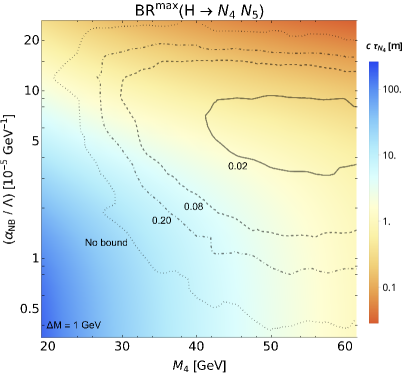
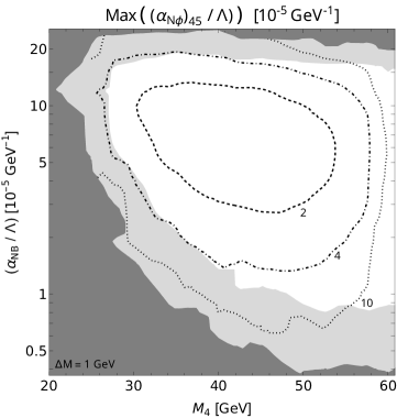
Figure 1: Left: Bounds on ${\rm BR}(H\to N_{4}\,N_{5})$, for $\Delta M=1\,$GeV. The coloured background gives the magnitude of the decay length of $N_{4}$. Right: Bounds on $(\alpha^{\prime}_{N\phi})_{45}/\Lambda$, for $\Delta M=1\,$GeV. Dark grey regions have no bound, while the light gray regions imply branching ratios larger than $20\%$.

In our first benchmark scenario, we consider $\Delta M=1\,$GeV. In this case, the prompt photon will carry very little $p_{T}$, so is unlikely to pass the selection cuts. We thus consider this benchmark as representative of all cases with very small $\Delta M$, as well as those with $H\to N_{4}\,N_{4}$ decays. Results are plotted in Figure 1. The left panel of the Figure shows our bounds on ${\rm BR}(H\to N_{4}\,N_{5})$, as contours on the $M_{4}-\alpha_{NB}/\Lambda$ plane. We find that the search is sensitive to the model for $M_{4}$ between 20 and 60 GeV, and $\alpha_{NB}/\Lambda$ between $0.4\times 10^{-5}\,\text{GeV}^{-1}$ and $2.2\times 10^{-4}\,$GeV^-1, approximately. In particular, we find a region where the branching ratio is constrained to be under $20\%$, which is below the bounds from ATLAS and CMS searches for Higgs decays to exotic undetected states [111, 112].

One can easily understand the sensitivity curves. First, from the point of view of $\alpha_{NB}/\Lambda$, values under $\sim 10^{-5}\,$GeV^-1 can have heavy neutrinos with a too long lifetime, such that most of them escape the detector without leaving a signal. In contrast, for values larger than $\sim 10^{-4}\,$GeV^-1, the $N_{4}$ decays much more promptly, which is reflected in our events being categorized in the smaller $|\Delta z_{\gamma}|$ and $t_{\gamma}$ bins, and thus not counted in the statistical analysis.

Moreover, for a fixed $\alpha_{NB}$, a small $M_{4}$ corresponds to a larger lifetime, increasing the possibility for the $N_{4}$ to escape the detector without leaving a signal. A large $M_{4}$, in contrast, also implies that the heavy neutrinos are produced with smaller momentum. Having a slow-moving parent leads to the photons being more delayed, which increases the number of events in the large $t_{\gamma}$ bin used in the analysis. Furthermore, the lower the momenta, the less collimated each neutrino - photon pair are, which favours having a large $|\Delta z_{\gamma}|$. However, in some regions of the parameter space, the mass cannot be arbitrarily large, as the $N_{4}\to\nu\,\gamma$ branching ratio can become smaller than unity, decreasing the overall final number of events.

On the left panel of the Figure we also show the decay length of $N_{4}$, with colours ranging from red ($c\tau\leq 0.1\,$m) to blue ($c\tau\geq 100\,$m). The (red) region with the smallest decay length corresponds to large $M_{4}$ and $\alpha_{NB}/\Lambda$, while the opposite side of the panel corresponds to the largest one (blue). The boundary between red and blue regions (in white) corresponds to a decay length around 1 m. Interestingly, for large $\alpha_{NB}/\Lambda$ this boundary crosses the plot diagonally, until it reaches values $\alpha_{NB}/\Lambda\lesssim 3\times 10^{-5}\,$GeV^-1. At this point, the boundary twists downwards, and proceeds vertically. This means that, within this region, the dipole operator is no longer the dominant contribution for the decay length, having a large component from the standard Seesaw partial width. Moreover, in this region the $N_{h}\to\nu\,\gamma$ branching ratio is strongly suppressed [37].

As can be seen in Equation (10), for given $M_{4},\,M_{5}$, the bounds on the Higgs branching ratios can be translated to constraints on the Anisimov-Graesser coefficient, $(\alpha^{\prime}_{N\phi})_{45}/\Lambda$. These are shown on the right panel of Figure 1. Here, the dark gray region corresponds to no bound on ${\rm BR}(H\to N_{4}\,N_{5})$, while for the light gray region the limit is above $20\%$, meaning that the searches in [111, 112] would give stronger bounds on the coefficient. Within the non-shaded region, $(\alpha^{\prime}_{N\phi})_{45}/\Lambda$ is limited to values of order $\sim 10^{-5}\,$GeV^-1. Notice that the area that constrains this coefficient most strongly is somewhat displaced to lighter masses with respect to the corresponding region for the branching ratio. The reason for this is that for large values of $M_{4}~{}\text{and}~{}M_{5}$ the Higgs branching ratio is naturally suppressed due to the smaller phase space, allowing for larger $\alpha^{\prime}_{N\phi}/\Lambda$.

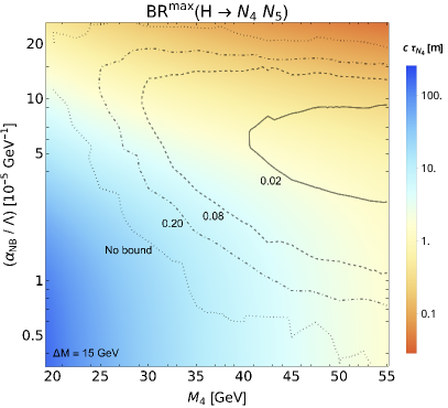
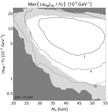
Figure 2: Same as Figure 1, but for $\Delta M=15\,$GeV.

Similarly, Figure 2 shows the same bounds, but for $\Delta M=15\,$GeV. This scenario differs from the previous one principally in the fact that the prompt photon from $N_{5}\to N_{4}\,\gamma$ decay will have a larger $p_{T}$, having thus better chances of passing the event selection than the one in the $\Delta M=1\,$GeV scenario. Notice this does not mean that this prompt photon will be used in the analysis, but rather that each event will be more likely to be assigned to the multi-photon channel.

On the left panel, we find that having a larger heavy neutrino mass difference tends to somewhat improve the sensitivity of the search with respect to the Higgs branching ratio, with the exclusion regions reaching smaller values of both $M_{4}$ and $\alpha_{NB/\Lambda}$. The reason for this is that, for fixed $M_{4}$, having a larger $M_{5}$ implies that the heavy neutrinos will have less momentum and, as argued earlier, this is correlated to larger $t_{\gamma}$ and $|\Delta z_{\gamma}|$ values.

On the right panel of Figure 2, we again show the constraints on $(\alpha^{\prime}_{N\phi})_{45}/\Lambda$. The sensitivity is very similar to that shown in Figure 1, with the regions slightly displaced towards larger values of $\alpha_{NB}/\Lambda$. This displacement implies that for larger $\alpha_{NB}/\Lambda$ the $\Delta M=15\,$GeV scenario is more sensitive than that for $\Delta M=1\,$GeV. However, for intermediate $\alpha_{NB}/\Lambda$, it turns out that the constraints on the branching ratio are slightly stronger for $\Delta M=1\,$GeV

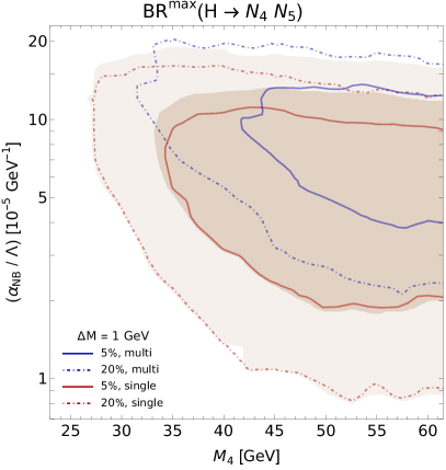
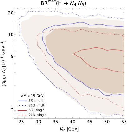
Figure 3: Comparison of single and multiphoton channels, shown in red and blue, respectively. Branching ratio limits of $5\%$ ($20\%$) are shown in solid (dashed-dotted) lines. Corresponding bounds using combined channels are shown in brown shading.

Perhaps more interestingly, in Figure 3 we compare the constraints on ${\rm BR}(H\to N_{4}\,N_{5})$ coming from the combined channel analysis, with those obtained separately from the single and multi-photon channels. The limits from the combined channel are shown as brown regions, while those from the single (multi-) photon channel are shown as red (blue) lines.

The scenario with $\Delta M=1\,$GeV is shown on the left. As expected, the region probed by the combined analysis comes from the union of regions probed by the individual channels. In particular, the multi-photon channel is most sensitive to regions with large $\alpha_{NB}/\Lambda$, while the single photon channel determines the sensitivity at low values. This is reasonable, the smaller $\alpha_{NB}/\Lambda$ is, the larger the chances that a heavy neutrino will escape the detector before decaying, removing one displaced photon from the analysis. Another reason for losing displaced photons at small $\alpha_{NB}/\Lambda$ is the suppressed $N_{4}\to\,\nu\,\gamma$ branching ratio.

It is interesting to note that in some regions the multi-photon channel is more sensitive than the combination. We attribute this, on the one hand, to the multi-photon channel having essentially no background, leading to a large sensitivity, and, on the other hand, to the combined analysis not including the per-bin information but just adding the events in both channels instead.

Finally, we turn to the right panel, which shows the scenario with $\Delta M=15\,$GeV. As commented before, the prompt photon from $N_{5}\to N_{4}\,\gamma$ is more likely to pass the selection. Thus, most events have one additional photon in comparison to $\Delta M=1\,$GeV, transferring displaced single photon events to the multi-photon channel. As commented before, since this channel has a much smaller background, the sensitivity is greater. Correspondingly, we have much less events on the single photon channel, leading to much milder constraints on the parameter space. Thus, it makes sense to have the combined analysis following the exclusion set by the multi-photon channel.

Before we conclude, it is important to comment on the interpretation of the results in the context of $\nu_{R}$SMEFT. As is well known, the effective operators can be generated from both perturbative and non-perturbative extensions of the Seesaw Lagrangian [7]. In particular, in perturbative extensions the dipole operator $\mathcal{O}_{NB}$ in Eq. (3) is generated from loop diagrams, which would lead to an extra factor $(4\pi)^{2}$ in the denominator. This leads to a rescaling of $(\alpha_{NB})/\Lambda$ by a factor $\sim 158$, meaning that, in a perturbative extension, our bounds would be applicable for $\Lambda$ around 100 GeV. Notice that since $(\alpha_{NB})/\Lambda$ only participates via the decay of the heavy neutrino, the energy scales involving this operator are of order $M_{4}$, meaning that the $\nu_{R}$SMEFT can still be applicable.

It is important to note that this does not necessarily mean that new physics beyond the $\nu_{R}$SMEFT should be expected at the 100 GeV scale. As a simple example of UV-completion, we consider the model in [113], which adds a scalar $\omega$ and a vector-like fermion $E$, transforming both only under $U(1)_{Y}$. In this model, for $m_{\omega}\ll m_{E}$, the dipole operator is in fact generated with a $1/m_{E}$ factor, with the implication that $m_{E}$ should be around 100 GeV. However, if $m_{\omega}\gg m_{E}$, the overall factor comes out as $m_{E}/m_{\omega}^{2}$, allowing for much larger masses while keeping $\Lambda$ at low values.

On the other hand, if the effective operators are generated in non-perturbative extensions, then these considerations need not to be taken into account. Thus, the bounds can be taken as shown without the need of rescaling. However, as commented in [38], in this scenario an explanation for the difference between $M_{N_{h}}$ and $\Lambda$ scales is lacking.

IV Conclusions

After more than 15 years in operation, the LHC has provided a huge amount of precious information. Searches such as the one studied in this work, probing the existence of LLPs, are a proof of the power and flexibility of this machine. It is thus essential to fully exploit all available data, in order to place bounds on new physics models.

To this end, we performed a detailed recast of the ATLAS search for displaced photons coming from LLP decays, triggered by a charged lepton associated to Higgs production [72]. This required the calculation of both non-pointing and time delay variables, $|\Delta z_{\gamma}|$ and $t_{\gamma}$. Apart from this, we refined the detector simulation beyond the standard settings in Delphes, implementing the isolation cuts, the resolutions, the efficiencies, and the overlap removal, reported by ATLAS for the search. We also reproduced the model-independent statistical analysis performed by the search.

With this in hand, we explored the sensitivity of the search to the Dimension-5 Seesaw Portal. Apart from the addition of sterile neutrinos, which generate light neutrino masses, this model includes two new $d=5$ effective operators featuring the sterile neutrinos themselves. The Anisimov-Graesser operator $\mathcal{O}_{N\phi}$, described by the parameter $\alpha_{N\phi}/\Lambda$, is an important contribution towards Higgs decay into the two heavy neutrinos. The dipole operator $\mathcal{O}_{NB}$, described by $\alpha_{NB}/\Lambda$, allows the heavy neutrinos to decay into photons and lighter neutrinos. Thus, in the region of parameter space where the heavy neutrinos have long lifetimes, the model can provide the final state the search is sensitive to.

As a result, we find that the search can constrain the branching ratio for Higgs decays into two heavy neutrinos, as long as the latter have masses between 20 and 60 GeV, and $\alpha_{NB}/\Lambda$ lies between $10^{-4}$ and $10^{-6}\,$GeV^-1. The bounds on the branching ratio can be as low as $2\%$. This in turn can be translated into limits on $\alpha_{N\phi}/\Lambda$, which can be constrained to values as small as $2\times 10^{-5}\,$GeV^-1.

In our work we also compare the sensitivity of the various channels used in the search. We find that, in general, the one photon channel is most sensitive to regions where the LLP lifetime is large, while the multi-photon channel is more appropriate for regions where the lifetime is shorter. However, this statement is modified in the presence of prompt photons generated along the LLPs, giving a much more important role to the multi-photon channel.

- [1] P. Minkowski, “ at a Rate of One Out of Muon Decays?,” Phys. Lett. B67 (1977) 421–428.
- [2] R. N. Mohapatra and G. Senjanovic, “Neutrino Mass and Spontaneous Parity Violation,” Phys. Rev. Lett. 44 (1980) 912.
- [3] T. Yanagida, “Horizontal Symmetry and Masses of Neutrinos,” Prog.Theor.Phys. 64 (1980) 1103.
- [4] M. Gell-Mann, P. Ramond, and R. Slansky, “Complex Spinors and Unified Theories,” Conf. Proc. C790927 (1979) 315–321, arXiv:1306.4669 [hep-th].
- [5] J. Schechter and J. W. F. Valle, “Neutrino Masses in SU(2) x U(1) Theories,” Phys. Rev. D22 (1980) 2227.
- [6] F. del Aguila, S. Bar-Shalom, A. Soni, and J. Wudka, “Heavy Majorana Neutrinos in the Effective Lagrangian Description: Application to Hadron Colliders,” Phys.Lett. B670 (2009) 399–402, arXiv:0806.0876 [hep-ph].
- [7] A. Aparici, K. Kim, A. Santamaria, and J. Wudka, “Right-handed neutrino magnetic moments,” Phys. Rev. D 80 (2009) 013010, arXiv:0904.3244 [hep-ph].
- [8] Y. Liao and X.-D. Ma, “Operators up to Dimension Seven in Standard Model Effective Field Theory Extended with Sterile Neutrinos,” Phys. Rev. D96 no. 1, (2017) 015012, arXiv:1612.04527 [hep-ph].
- [9] S. Bhattacharya and J. Wudka, “Dimension-seven operators in the standard model with right handed neutrinos,” Phys. Rev. D94 no. 5, (2016) 055022, arXiv:1505.05264 [hep-ph]. [Erratum: Phys. Rev.D95,no.3,039904(2017)].
- [10] H.-L. Li, Z. Ren, M.-L. Xiao, J.-H. Yu, and Y.-H. Zheng, “Operator bases in effective field theories with sterile neutrinos: d 9,” JHEP 11 (2021) 003, arXiv:2105.09329 [hep-ph].
- [11] L. Duarte, J. Peressutti, and O. A. Sampayo, “Majorana neutrino decay in an Effective Approach,” Phys. Rev. D92 no. 9, (2015) 093002, arXiv:1508.01588 [hep-ph].
- [12] L. Duarte, I. Romero, J. Peressutti, and O. A. Sampayo, “Effective Majorana neutrino decay,” Eur. Phys. J. C 76 no. 8, (2016) 453, arXiv:1603.08052 [hep-ph].
- [13] L. Duarte, J. Peressutti, and O. A. Sampayo, “Not-that-heavy Majorana neutrino signals at the LHC,” J. Phys. G 45 no. 2, (2018) 025001, arXiv:1610.03894 [hep-ph].
- [14] A. Caputo, P. Hernandez, J. Lopez-Pavon, and J. Salvado, “The seesaw portal in testable models of neutrino masses,” JHEP 06 (2017) 112, arXiv:1704.08721 [hep-ph].
- [15] L. Duarte, G. Zapata, and O. A. Sampayo, “Angular and polarization trails from effective interactions of Majorana neutrinos at the LHeC,” Eur. Phys. J. C78 no. 5, (2018) 352, arXiv:1802.07620 [hep-ph].
- [16] C.-X. Yue and J.-P. Chu, “Sterile neutrino and leptonic decays of the pseudoscalar mesons,” Phys. Rev. D 98 no. 5, (2018) 055012, arXiv:1808.09139 [hep-ph].
- [17] L. Duarte, G. Zapata, and O. A. Sampayo, “Final taus and initial state polarization signatures from effective interactions of Majorana neutrinos at future colliders,” Eur. Phys. J. C79 no. 3, (2019) 240, arXiv:1812.01154 [hep-ph].
- [18] L. Duarte, J. Peressutti, I. Romero, and O. A. Sampayo, “Majorana neutrinos with effective interactions in B decays,” Eur. Phys. J. C79 no. 7, (2019) 593, arXiv:1904.07175 [hep-ph].
- [19] I. Bischer and W. Rodejohann, “General neutrino interactions from an effective field theory perspective,” Nucl. Phys. B 947 (2019) 114746, arXiv:1905.08699 [hep-ph].
- [20] J. Alcaide, S. Banerjee, M. Chala, and A. Titov, “Probes of the Standard Model effective field theory extended with a right-handed neutrino,” JHEP 08 (2019) 031, arXiv:1905.11375 [hep-ph].
- [21] J. M. Butterworth, M. Chala, C. Englert, M. Spannowsky, and A. Titov, “Higgs phenomenology as a probe of sterile neutrinos,” Phys. Rev. D 100 no. 11, (2019) 115019, arXiv:1909.04665 [hep-ph].
- [22] J. Jones-Pérez, J. Masias, and J. Ruiz-Álvarez, “Search for Long-Lived Heavy Neutrinos at the LHC with a VBF Trigger,” Eur. Phys. J. C 80 no. 7, (2020) 642, arXiv:1912.08206 [hep-ph].
- [23] M. Chala and A. Titov, “One-loop matching in the SMEFT extended with a sterile neutrino,” JHEP 05 (2020) 139, arXiv:2001.07732 [hep-ph].
- [24] W. Dekens, J. de Vries, K. Fuyuto, E. Mereghetti, and G. Zhou, “Sterile neutrinos and neutrinoless double beta decay in effective field theory,” JHEP 06 (2020) 097, arXiv:2002.07182 [hep-ph].
- [25] D. Barducci, E. Bertuzzo, A. Caputo, and P. Hernandez, “Minimal flavor violation in the see-saw portal,” JHEP 06 (2020) 185, arXiv:2003.08391 [hep-ph].
- [26] L. Duarte, G. Zapata, and O. Sampayo, “Angular and polarization observables for Majorana-mediated B decays with effective interactions,” Eur. Phys. J. C 80 no. 9, (2020) 896, arXiv:2006.11216 [hep-ph].
- [27] A. Biekötter, M. Chala, and M. Spannowsky, “The effective field theory of low scale see-saw at colliders,” Eur. Phys. J. C 80 no. 8, (2020) 743, arXiv:2007.00673 [hep-ph].
- [28] J. De Vries, H. K. Dreiner, J. Y. Günther, Z. S. Wang, and G. Zhou, “Long-lived Sterile Neutrinos at the LHC in Effective Field Theory,” JHEP 03 (2021) 148, arXiv:2010.07305 [hep-ph].
- [29] D. Barducci, E. Bertuzzo, A. Caputo, P. Hernandez, and B. Mele, “The see-saw portal at future Higgs Factories,” JHEP 03 (2021) 117, arXiv:2011.04725 [hep-ph].
- [30] W. Dekens, J. de Vries, and T. Tong, “Sterile neutrinos with non-standard interactions in - and 0-decay experiments,” JHEP 08 (2021) 128, arXiv:2104.00140 [hep-ph].
- [31] V. Cirigliano, W. Dekens, J. de Vries, K. Fuyuto, E. Mereghetti, and R. Ruiz, “Leptonic anomalous magnetic moments in SMEFT,” JHEP 08 (2021) 103, arXiv:2105.11462 [hep-ph].
- [32] G. Cottin, J. C. Helo, M. Hirsch, A. Titov, and Z. S. Wang, “Heavy neutral leptons in effective field theory and the high-luminosity LHC,” JHEP 09 (2021) 039, arXiv:2105.13851 [hep-ph].
- [33] R. Beltrán, G. Cottin, J. C. Helo, M. Hirsch, A. Titov, and Z. S. Wang, “Long-lived heavy neutral leptons at the LHC: four-fermion single-NR operators,” JHEP 01 (2022) 044, arXiv:2110.15096 [hep-ph].
- [34] G. Zhou, J. Y. Günther, Z. S. Wang, J. de Vries, and H. K. Dreiner, “Long-lived sterile neutrinos at Belle II in effective field theory,” JHEP 04 (2022) 057, arXiv:2111.04403 [hep-ph].
- [35] G. Zhou, “Light sterile neutrinos and lepton-number-violating kaon decays in effective field theory,” JHEP 06 (2022) 127, arXiv:2112.00767 [hep-ph].
- [36] R. Beltrán, G. Cottin, J. C. Helo, M. Hirsch, A. Titov, and Z. S. Wang, “Long-lived heavy neutral leptons from mesons in effective field theory,” JHEP 01 (2023) 015, arXiv:2210.02461 [hep-ph].
- [37] F. Delgado, L. Duarte, J. Jones-Perez, C. Manrique-Chavil, and S. Peña, “Assessment of the dimension-5 seesaw portal and impact of exotic Higgs decays on non-pointing photon searches,” JHEP 09 (2022) 079, arXiv:2205.13550 [hep-ph].
- [38] D. Barducci, E. Bertuzzo, M. Taoso, and C. Toni, “Probing right-handed neutrinos dipole operators,” JHEP 03 (2023) 239, arXiv:2209.13469 [hep-ph].
- [39] G. Zapata, T. Urruzola, O. A. Sampayo, and L. Duarte, “Lepton collider probes for Majorana neutrino effective interactions,” Eur. Phys. J. C 82 no. 6, (2022) 544, arXiv:2201.02480 [hep-ph].
- [40] D. Barducci and E. Bertuzzo, “The see-saw portal at future Higgs factories: the role of dimension six operators,” JHEP 06 (2022) 077, arXiv:2201.11754 [hep-ph].
- [41] M. Mitra, S. Mandal, R. Padhan, A. Sarkar, and M. Spannowsky, “Reexamining right-handed neutrino EFTs up to dimension six,” Phys. Rev. D 106 no. 11, (2022) 113008, arXiv:2210.12404 [hep-ph].
- [42] E. Fernández-Martínez, M. González-López, J. Hernández-García, M. Hostert, and J. López-Pavón, “Effective portals to heavy neutral leptons,” JHEP 09 (2023) 001, arXiv:2304.06772 [hep-ph].
- [43] R. Beltrán, R. Cepedello, and M. Hirsch, “Tree-level UV completions for SMEFT and operators,” JHEP 08 (2023) 166, arXiv:2306.12578 [hep-ph].
- [44] G. Zapata, T. Urruzola, O. A. Sampayo, and L. Duarte, “Sensitivity prospects for lepton-trijet signals in the SMEFT at the LHeC,” arXiv:2305.16991 [hep-ph].
- [45] R. Beltrán, J. Günther, M. Hirsch, A. Titov, and Z. S. Wang, “Heavy neutral leptons from kaons in effective field theory,” arXiv:2309.11546 [hep-ph].
- [46] J. Y. Günther, J. de Vries, H. K. Dreiner, Z. S. Wang, and G. Zhou, “Long-lived neutral fermions at the DUNE near detector,” arXiv:2310.12392 [hep-ph].
- [47] F. F. Deppisch, P. S. Bhupal Dev, and A. Pilaftsis, “Neutrinos and Collider Physics,” New J. Phys. 17 no. 7, (2015) 075019, arXiv:1502.06541 [hep-ph].
- [48] S. Antusch, E. Cazzato, and O. Fischer, “Sterile neutrino searches at future , , and colliders,” Int. J. Mod. Phys. A 32 no. 14, (2017) 1750078, arXiv:1612.02728 [hep-ph].
- [49] A. M. Abdullahi et al., “The Present and Future Status of Heavy Neutral Leptons,” in 2022 Snowmass Summer Study. 3, 2022. arXiv:2203.08039 [hep-ph].
- [50] N. W. Kamp, M. Hostert, A. Schneider, S. Vergani, C. A. Argüelles, J. M. Conrad, M. H. Shaevitz, and M. A. Uchida, “Dipole-coupled heavy-neutral-lepton explanations of the MiniBooNE excess including constraints from MINERvA data,” Phys. Rev. D 107 no. 5, (2023) 055009, arXiv:2206.07100 [hep-ph].
- [51] A. M. Abdullahi, J. Hoefken Zink, M. Hostert, D. Massaro, and S. Pascoli, “A panorama of new-physics explanations to the MiniBooNE excess,” arXiv:2308.02543 [hep-ph].
- [52] G. Magill, R. Plestid, M. Pospelov, and Y.-D. Tsai, “Dipole Portal to Heavy Neutral Leptons,” Phys. Rev. D 98 no. 11, (2018) 115015, arXiv:1803.03262 [hep-ph].
- [53] T. Schwetz, A. Zhou, and J.-Y. Zhu, “Constraining active-sterile neutrino transition magnetic moments at DUNE near and far detectors,” JHEP 21 (2020) 200, arXiv:2105.09699 [hep-ph].
- [54] V. Brdar, A. Greljo, J. Kopp, and T. Opferkuch, “The Neutrino Magnetic Moment Portal: Cosmology, Astrophysics, and Direct Detection,” JCAP 01 (2021) 039, arXiv:2007.15563 [hep-ph].
- [55] V. Brdar, A. de Gouvêa, Y.-Y. Li, and P. A. N. Machado, “Neutrino magnetic moment portal and supernovae: New constraints and multimessenger opportunities,” Phys. Rev. D 107 no. 7, (2023) 073005, arXiv:2302.10965 [hep-ph].
- [56] M. Ovchynnikov, T. Schwetz, and J.-Y. Zhu, “Dipole portal and neutrinophilic scalars at DUNE revisited: The importance of the high-energy neutrino tail,” Phys. Rev. D 107 no. 5, (2023) 055029, arXiv:2210.13141 [hep-ph].
- [57] M. Ovchynnikov and J.-Y. Zhu, “Search for the dipole portal of heavy neutral leptons at future colliders,” JHEP 07 (2023) 039, arXiv:2301.08592 [hep-ph].
- [58] Y. Zhang, M. Song, R. Ding, and L. Chen, “Neutrino dipole portal at electron colliders,” Phys. Lett. B 829 (2022) 137116, arXiv:2204.07802 [hep-ph].
- [59] Y. Zhang and W. Liu, “Probing active-sterile neutrino transition magnetic moments at LEP and CEPC,” Phys. Rev. D 107 no. 9, (2023) 095031, arXiv:2301.06050 [hep-ph].
- [60] W. Liu and Y. Zhang, “Testing neutrino dipole portal by long-lived particle detectors at the LHC,” Eur. Phys. J. C 83 no. 7, (2023) 568, arXiv:2302.02081 [hep-ph].
- [61] D. Barducci, W. Liu, A. Titov, Z. S. Wang, and Y. Zhang, “Probing the dipole portal to heavy neutral leptons via meson decays at the high-luminosity LHC,” arXiv:2308.16608 [hep-ph].
- [62] G.-y. Huang, S. Jana, M. Lindner, and W. Rodejohann, “Probing heavy sterile neutrinos at neutrino telescopes via the dipole portal,” Phys. Lett. B 840 (2023) 137842, arXiv:2204.10347 [hep-ph].
- [63] A. Pilaftsis, “Radiatively induced neutrino masses and large Higgs neutrino couplings in the standard model with Majorana fields,” Z. Phys. C 55 (1992) 275–282, arXiv:hep-ph/9901206.
- [64] P. S. Bhupal Dev, R. Franceschini, and R. N. Mohapatra, “Bounds on TeV Seesaw Models from LHC Higgs Data,” Phys. Rev. D 86 (2012) 093010, arXiv:1207.2756 [hep-ph].
- [65] C. G. Cely, A. Ibarra, E. Molinaro, and S. T. Petcov, “Higgs Decays in the Low Scale Type I See-Saw Model,” Phys. Lett. B 718 (2013) 957–964, arXiv:1208.3654 [hep-ph].
- [66] A. M. Gago, P. Hernández, J. Jones-Pérez, M. Losada, and A. Moreno Briceño, “Probing the Type I Seesaw Mechanism with Displaced Vertices at the LHC,” Eur. Phys. J. C75 no. 10, (2015) 470, arXiv:1505.05880 [hep-ph].
- [67] A. Das, P. S. B. Dev, and C. S. Kim, “Constraining Sterile Neutrinos from Precision Higgs Data,” Phys. Rev. D 95 no. 11, (2017) 115013, arXiv:1704.00880 [hep-ph].
- [68] A. Maiezza, M. Nemevšek, and F. Nesti, “Lepton Number Violation in Higgs Decay at LHC,” Phys. Rev. Lett. 115 (2015) 081802, arXiv:1503.06834 [hep-ph].
- [69] F. F. Deppisch, W. Liu, and M. Mitra, “Long-lived Heavy Neutrinos from Higgs Decays,” JHEP 08 (2018) 181, arXiv:1804.04075 [hep-ph].
- [70] E. Accomando, L. Delle Rose, S. Moretti, E. Olaiya, and C. H. Shepherd-Themistocleous, “Novel SM-like Higgs decay into displaced heavy neutrino pairs in U(1)’ models,” JHEP 04 (2017) 081, arXiv:1612.05977 [hep-ph].
- [71] J. D. Mason, “Time-Delayed Electrons from Higgs Decays to Right-Handed Neutrinos,” JHEP 07 (2019) 089, arXiv:1905.07772 [hep-ph].
- [72] ATLAS Collaboration, G. Aad et al., “Search for displaced photons produced in exotic decays of the Higgs boson using 13 TeV pp collisions with the ATLAS detector,” Phys. Rev. D 108 no. 3, (2023) 032016, arXiv:2209.01029 [hep-ex].
- [73] M. Blennow, E. Fernández-Martínez, J. Hernández-García, J. López-Pavón, X. Marcano, and D. Naredo-Tuero, “Bounds on lepton non-unitarity and heavy neutrino mixing,” JHEP 08 (2023) 030, arXiv:2306.01040 [hep-ph].
- [74] S. Weinberg, “Baryon and Lepton Nonconserving Processes,” Phys. Rev. Lett. 43 (1979) 1566–1570.
- [75] A. Anisimov, “Majorana Dark Matter,” in 6th International Workshop on the Identification of Dark Matter, pp. 439–449. 12, 2006. arXiv:hep-ph/0612024.
- [76] M. L. Graesser, “Broadening the Higgs boson with right-handed neutrinos and a higher dimension operator at the electroweak scale,” Phys. Rev. D 76 (2007) 075006, arXiv:0704.0438 [hep-ph].
- [77] M. L. Graesser, “Experimental Constraints on Higgs Boson Decays to TeV-scale Right-Handed Neutrinos,” arXiv:0705.2190 [hep-ph].
- [78] A. Atre, T. Han, S. Pascoli, and B. Zhang, “The Search for Heavy Majorana Neutrinos,” JHEP 0905 (2009) 030, arXiv:0901.3589 [hep-ph].
- [79] S. Kovalenko, Z. Lu, and I. Schmidt, “Lepton Number Violating Processes Mediated by Majorana Neutrinos at Hadron Colliders,” Phys. Rev. D 80 (2009) 073014, arXiv:0907.2533 [hep-ph].
- [80] J. C. Helo, S. Kovalenko, and I. Schmidt, “Sterile neutrinos in lepton number and lepton flavor violating decays,” Nucl. Phys. B 853 (2011) 80–104, arXiv:1005.1607 [hep-ph].
- [81] K. Bondarenko, A. Boyarsky, D. Gorbunov, and O. Ruchayskiy, “Phenomenology of GeV-scale Heavy Neutral Leptons,” JHEP 11 (2018) 032, arXiv:1805.08567 [hep-ph].
- [82] P. Coloma, E. Fernández-Martínez, M. González-López, J. Hernández-García, and Z. Pavlovic, “GeV-scale neutrinos: interactions with mesons and DUNE sensitivity,” Eur. Phys. J. C 81 no. 1, (2021) 78, arXiv:2007.03701 [hep-ph].
- [83] G. C. Branco, W. Grimus, and L. Lavoura, “The Seesaw Mechanism in the Presence of a Conserved Lepton Number,” Nucl. Phys. B 312 (1989) 492–508.
- [84] M. Shaposhnikov, “A Possible symmetry of the nuMSM,” Nucl. Phys. B 763 (2007) 49–59, arXiv:hep-ph/0605047.
- [85] J. Kersten and A. Y. Smirnov, “Right-Handed Neutrinos at CERN LHC and the Mechanism of Neutrino Mass Generation,” Phys. Rev. D 76 (2007) 073005, arXiv:0705.3221 [hep-ph].
- [86] M. B. Gavela, T. Hambye, D. Hernandez, and P. Hernandez, “Minimal Flavour Seesaw Models,” JHEP 09 (2009) 038, arXiv:0906.1461 [hep-ph].
- [87] P. Hernández, J. Jones-Pérez, and O. Suarez-Navarro, “Majorana vs Pseudo-Dirac Neutrinos at the ILC,” Eur. Phys. J. C 79 no. 3, (2019) 220, arXiv:1810.07210 [hep-ph].
- [88] D. Wyler and L. Wolfenstein, “Massless Neutrinos in Left-Right Symmetric Models,” Nucl. Phys. B 218 (1983) 205–214.
- [89] R. N. Mohapatra and J. W. F. Valle, “Neutrino Mass and Baryon Number Nonconservation in Superstring Models,” Phys. Rev. D34 (1986) 1642.
- [90] M. Malinsky, J. C. Romao, and J. W. F. Valle, “Novel supersymmetric SO(10) seesaw mechanism,” Phys. Rev. Lett. 95 (2005) 161801, arXiv:hep-ph/0506296.
- [91] S. K. Kang and C. S. Kim, “Extended double seesaw model for neutrino mass spectrum and low scale leptogenesis,” Phys. Lett. B 646 (2007) 248–252, arXiv:hep-ph/0607072.
- [92] S. Antusch, E. Cazzato, and O. Fischer, “Resolvable heavy neutrino–antineutrino oscillations at colliders,” Mod. Phys. Lett. A 34 no. 07n08, (2019) 1950061, arXiv:1709.03797 [hep-ph].
- [93] E. Fernández-Martínez, X. Marcano, and D. Naredo-Tuero, “HNL mass degeneracy: implications for low-scale seesaws, LNV at colliders and leptogenesis,” JHEP 03 (2023) 057, arXiv:2209.04461 [hep-ph].
- [94] J. Alwall, R. Frederix, S. Frixione, V. Hirschi, F. Maltoni, O. Mattelaer, H. S. Shao, T. Stelzer, P. Torrielli, and M. Zaro, “The automated computation of tree-level and next-to-leading order differential cross sections, and their matching to parton shower simulations,” JHEP 07 (2014) 079, arXiv:1405.0301 [hep-ph].
- [95] A. Buckley, J. Ferrando, S. Lloyd, K. Nordström, B. Page, M. Rüfenacht, M. Schönherr, and G. Watt, “LHAPDF6: parton density access in the LHC precision era,” Eur. Phys. J. C 75 (2015) 132, arXiv:1412.7420 [hep-ph].
- [96] N. D. Christensen and C. Duhr, “FeynRules - Feynman rules made easy,” Comput. Phys. Commun. 180 (2009) 1614–1641, arXiv:0806.4194 [hep-ph].
- [97] A. Alloul, N. D. Christensen, C. Degrande, C. Duhr, and B. Fuks, “FeynRules 2.0 - A complete toolbox for tree-level phenomenology,” Comput. Phys. Commun. 185 (2014) 2250–2300, arXiv:1310.1921 [hep-ph].
- [98] T. Sjostrand, S. Mrenna, and P. Z. Skands, “PYTHIA 6.4 Physics and Manual,” JHEP 05 (2006) 026, arXiv:hep-ph/0603175 [hep-ph].
- [99] M. Dobbs and J. B. Hansen, “The HepMC C++ Monte Carlo event record for High Energy Physics,” Comput. Phys. Commun. 134 (2001) 41–46.
- [100] A. Buckley, P. Ilten, D. Konstantinov, L. Lönnblad, J. Monk, W. Pokorski, T. Przedzinski, and A. Verbytskyi, “The HepMC3 event record library for Monte Carlo event generators,” Comput. Phys. Commun. 260 (2021) 107310, arXiv:1912.08005 [hep-ph].
- [101] LHC Higgs Cross Section Working Group Collaboration, D. de Florian et al., “Handbook of LHC Higgs Cross Sections: 4. Deciphering the Nature of the Higgs Sector,” arXiv:1610.07922 [hep-ph].
- [102] F. Delgado, “Búsqueda de neutrinos pesados via fotones fuera de tiempo en colisionadores,” February, 2023. Available at http://hdl.handle.net/20.500.12404/24286.
- [103] DELPHES 3 Collaboration, J. de Favereau, C. Delaere, P. Demin, A. Giammanco, V. Lemaître, A. Mertens, and M. Selvaggi, “DELPHES 3, A modular framework for fast simulation of a generic collider experiment,” JHEP 02 (2014) 057, arXiv:1307.6346 [hep-ex].
- [104] M. Cacciari, G. P. Salam, and G. Soyez, “FastJet User Manual,” Eur. Phys. J. C72 (2012) 1896, arXiv:1111.6097 [hep-ph].
- [105] ATLAS Collaboration, G. Aad et al., “The ATLAS Experiment at the CERN Large Hadron Collider,” JINST 3 (2008) S08003.
- [106] ATLAS Collaboration, G. Aad et al., “Search for nonpointing and delayed photons in the diphoton and missing transverse momentum final state in 8 TeV collisions at the LHC using the ATLAS detector,” Phys. Rev. D 90 no. 11, (2014) 112005, arXiv:1409.5542 [hep-ex].
- [107] ATLAS Collaboration, G. Aad et al., “Electron and photon performance measurements with the ATLAS detector using the 2015–2017 LHC proton-proton collision data,” JINST 14 no. 12, (2019) P12006, arXiv:1908.00005 [hep-ex].
- [108] ATLAS Collaboration, G. Aad et al., “Muon reconstruction and identification efficiency in ATLAS using the full Run 2 collision data set at TeV,” Eur. Phys. J. C 81 no. 7, (2021) 578, arXiv:2012.00578 [hep-ex].
- [109] A. L. Read, “Presentation of search results: The CL(s) technique,” J. Phys. G28 (2002) 2693–2704. [,11(2002)].
- [110] Particle Data Group Collaboration, R. L. Workman et al., “Review of Particle Physics,” PTEP 2022 (2022) 083C01.
- [111] CMS Collaboration, A. M. Sirunyan et al., “Combined measurements of Higgs boson couplings in proton–proton collisions at ,” Eur. Phys. J. C 79 no. 5, (2019) 421, arXiv:1809.10733 [hep-ex].
- [112] ATLAS Collaboration, G. Aad et al., “Combined measurements of Higgs boson production and decay using up to fb-1 of proton-proton collision data at 13 TeV collected with the ATLAS experiment,” Phys. Rev. D 101 no. 1, (2020) 012002, arXiv:1909.02845 [hep-ex].
- [113] A. Aparici, A. Santamaria, and J. Wudka, “A model for right-handed neutrino magnetic moments,” J. Phys. G 37 (2010) 075012, arXiv:0911.4103 [hep-ph].