Distance-coupling as an Approach to Position and Formation Control

Abstract

Studies of coordinated motion in autonomous vehicle groups have become a significant topic of interest in recent years. In this paper, we study the case when the agents are limited to distance measurements from predetermined reference points, or anchors. A novel approach, referred to as distance-coupling, is proposed for approximating agent positions from anchor distances. By taking the difference between squared distance functions, we cancel out the quadratic term and obtain a linear function of the position for the point of interest. We apply this method to the homing problem and prove Lyapunov stability with and without anchor placement error; defining bounds on the region of attraction when the anchors are linearly transformed from their desired positions. To further increase complexity, we show how the policy can be implemented on the formation control problem for a set of autonomous agents. In this context, we prove the existence of the set of equilibria for the distance-coupled formation controller and make preliminary claims on its convergence. The performance for both controllers are subsequently validated through simulation.

I Introduction

Autonomously operated vehicles are commonly designed around high-cost measurement devices used for real-time localization. However, there exists instances, especially in low-cost systems, where the measurements available to the agents are limited to basic geometric information. We study the case when the information available is restricted to its Euclidean distance from $p$ fixed points, or anchors. Exploiting a linear, first-order model, we first address the homing problem. In this case, the primary goal is to move an agent from an arbitrary initial position to some predetermined equilibrium position using the available measurement data. Despite being based on nonlinear measurements, our controller is a simple linear function, and its stability can be proven in a straight-forward manner.

We also consider the problem of driving $m=p$ agents into some predetermined formation using only inter-agent distances. In this case, we show that the controller defined for the homing problem can be implemented with minimal adjustments. Subsequently, the set of equilibrium positions are proven through transformation invariance, and validated through simulation.

I-A Literature Review

Studies of distance-based position functions have primarily been investigated through barycentric coordinates [1]. These methods represent the positions of anchors as vertices of a polygon and utilize its geometry to derive the agent’s position. While this method is robust in many applications, the point is usually limited to the bounds of a convex polyhedron and maintains ill-defined behaviors when this assumption is broken. To overcome this, researchers have implemented policy switching schemes to the formation control problem with success in 2-D [2] and 3-D [3] coordinate frames.

For distance-based formation control, the most popular approach uses gradient-descent over a function defined on the measurement graph [4, 5]. The graph can take many forms (directed/undirected, fully connected, etc.), but the connections are predetermined and static. Papers by Lin, Dimarogonas and Choi are also among the first to demonstrate the stability of assorted gradient-based formation control policies through standard analysis methods [6, 7, 8].

Another noteworthy example is that of [9] which is among the first written on the topic and discusses a catalog of analytical, methods which can be used to stabilize formations within small perturbations of their equilibrium. Lastly, the papers [10, 11] discuss the formation control of second-order systems, and [12] defines a policy in terms of the complex Laplacian. The review paper [13] lays a good foundation for many of the methods available. In addition to formation control in a distance-based context, it also discusses methods for the position and displacement-based measurement cases.

I-B Paper Contributions

In this paper, we present a new method that algebraically cancels the nonlinear term from available distance functions. By taking the difference between squared-distance measurements, we show that we can accurately construct a linear approximation of the agent’s position in the environment. We refer to this method as distance-coupling.

The distance-coupled approach is novel in comparison to the literature as it does not have strict requirements on agent positions similar to those found in barycentric coordinate methods. Where preexisting methods primarily depend on the convexity of the anchor environment, our approach makes no such claims and allows the user to select anchor positions which are non-convex. However, we discuss degenerate collinearity cases and the minimum number of anchors required (Section III-A).

The new approach also enjoys better convergence expectations then the gradient-based alternative. For the homing problem, we prove that the linear controller exhibits global exponential convergence in the ideal case and a sufficiently large region of attraction when the anchors are linearly offset from their desired positions. For the formation control problem, we formally characterize the set of all equilibria through the controller’s transformation invariance, and confirm large regions of attraction empirically.

While we demonstrate our results in an $\mathbb{R}^{2}$ environment for simplicity, the methods discussed in Section III are generalized to $\mathbb{R}^{n}$.

II System Definition

We start by defining the agent dynamics and ideal controller, along with the measurements available to the system.

II-A System Dynamics

The agents are modeled as a linear, time-invariant single integrator of the form

$$\dot{x}=u,$$ (1)

where $x\in\mathbb{R}^{n}$ and $u\in\mathbb{R}^{n}$ are the state and the control input, respectively. As common in the literature, we assume that the environment is unbounded and without obstacles. The goal of the homing problem is to move an agent from some initial condition to an equilibrium position denoted by $x^{(\text{eq})}$.

For the case that there are $m$-agents operating in a single environment, we can write (1) in matrix form such that

$$\dot{X}=U,$$ (2)

where $X\in\mathbb{R}^{n\times m}$ and $U\in\mathbb{R}^{n\times m}$ are the state and control for the set of agents defined by

$$X=\begin{bmatrix}x_{1}&\cdots&x_{m}\end{bmatrix}\text{, and }U=\begin{bmatrix}u_{1}&\cdots&u_{m}\end{bmatrix}.$$ (3)

II-B Ideal Controller

Since the system is linear, we define a simple state feedback controller that brings the agent to the goal position $x^{(\text{eq})}\in\mathbb{R}^{n}$ as

$$u(x)=C(x-x^{(\text{eq})}),$$ (4)

where $C\in\mathbb{R}^{n\times n}$ describes the policy coefficients. By standard linear system theory, if $C$ has eigenvalues with negative real parts, then the system is globally exponentially stable and the state will converge to the desired equilibrium from any initial condition [14].

Unfortunately, we are limited to the measurements described in the next section and cannot define a direct controller from the state of the agent. That said, (4) will be referred to as the ideal control.

II-C Anchor and Anchor-distance Sets

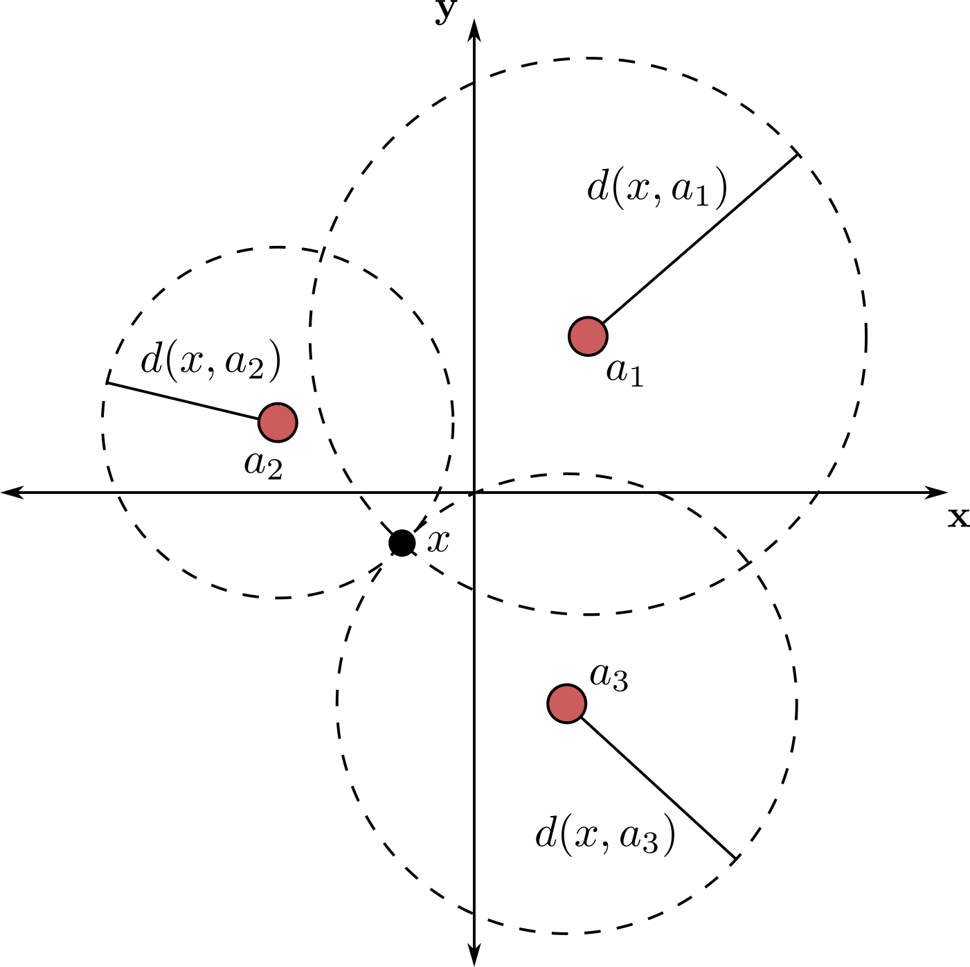
Figure 1: Anchor set where $p=3$ so that $\mathcal{A}=\{a_{1},a_{2},a_{3}\}$ and $\mathcal{D}(x,A)=\{d(x,a_{1}),d(x,a_{2}),d(x,a_{3})\}$.

We assume the presence of $p$-anchors which are represented by the set

$$\mathcal{A}=\{a_{i}\in\mathbb{R}^{n}:\forall i\leq p\},$$ (5)

where $a_{i}$ is the position of the $i$-th anchor. We assume that the agent measures the distance from its position to each of the anchors. The anchor-distance set is thus defined as

$$\mathcal{D}(x,\mathcal{A})=\{d(x,a_{i})\in\mathbb{R}:a_{i}\in\mathcal{A}\},$$ (6)

where

$$d(x,a_{i})=\sqrt{(x-a_{i})^{\intercal}(x-a_{i})}.$$ (7)

An example for when $p=3$ is shown in Figure 1. In the interest of conciseness, the individual distance functions from the point $x$ are referred to as $d_{i}(x)=d(x,a_{i})$, and the anchor-distance set is referred to as $\mathcal{D}(x)=\mathcal{D}(x,\mathcal{A})$.

III Distance-coupled Position Control

In this section we show how (4) can be indirectly implemented as a function of the measurement set $\mathcal{D}(x)$ via distance-coupled functions. We then prove Lyapunov stability, characterize the region of attraction when the anchors are linearly transformed and show the behavior of the closed-loop system in simulation.

III-A Distance-coupled Position and Control

We start by squaring and expanding each element of the anchor-distance set (6) which results in

$$d_{i}^{2}(x) =(x-a_{i})^{\intercal}(x-a_{i})$$ (8)

$$=x^{\intercal}x-2x^{\intercal}a_{i}+a_{i}^{\intercal}a_{i}.$$

The key step in our approach is to note that by subtracting the squared-distance functions for two anchors, the quadratic terms $x^{\intercal}x$ cancel out such that

$$d_{i}^{2}(x)-d_{j}^{2}(x)= \ (x^{\intercal}x-2x^{\intercal}a_{i}+a_{i}^{\intercal}a_{i})$$ (9)

$$-(x^{\intercal}x-2x^{\intercal}a_{j}+a_{j}^{\intercal}a_{j})$$

$$= -2x^{\intercal}(a_{i}-a_{j})+a_{i}^{\intercal}a_{i}-a_{j}^{\intercal}a_{j}.$$

Moving the state-related terms to the left we obtain

$$-2(a_{i}-a_{j})^{\intercal}x=d_{i}^{2}(x)-d_{j}^{2}(x)-a_{i}^{\intercal}a_{i}+a_{j}^{\intercal}a_{j}.$$ (10)

We reorganize the terms in (10) in matrix form with the intent of obtaining an expression for the full state $x$ through a linear system of equations:

$$A =\text{vstack}(\{-2(a_{i}-a_{j})^{\intercal}:\forall(i,j)\in\mathcal{I}\}),$$ (11)

$$b =\text{vstack}(\{a_{i}^{\intercal}a_{i}-a_{j}^{\intercal}a_{j}:\forall(i,j)\in\mathcal{I}\}),$$

$$h(x) =\text{vstack}(\{d_{i}^{2}(x)-d_{j}^{2}(x):\forall(i,j)\in\mathcal{I}\}),$$

where $\mathcal{I}$ is the set of $(i,j)$ indices which make up every combination of the anchors included in (5). The vstack$(\cdot)$ function simply converts a set of values into a vertically-oriented vector/matrix as appropriate. Using $|\mathcal{I}|$ to denote the cardinality of $\mathcal{I}$, we then have that $A\in\mathbb{R}^{|\mathcal{I}|\times n}$, and the vectors $b,h(x)\in\mathbb{R}^{|\mathcal{I}|}$.

Combining these with (10), the distance-coupled position of the agent can be computed by solving the linear system:

$$Ax=h(x)-b$$ (12)

$$\Rightarrow A^{\intercal}Ax=A^{\intercal}(h(x)-b)$$

$$\>\begin{aligned} \Rightarrow x&=(A^{\intercal}A)^{-1}A^{\intercal}(h(x)-b)\\ &=K(h(x)-b),\end{aligned}$$

where $K=(A^{\intercal}A)^{-1}A^{\intercal}$. Since the matrix $A^{\intercal}A$ is by definition positive definite, it is invertible if $A$ has full column rank with a subset of $n+1$ noncollinear anchor positions. While we do not include the proof here for conciseness, it is trivial and follows from standard linear algebra theory.

We refer to (12) as the distance-coupled position and can substitute it into (4) to obtain the corresponding distance-coupled controller:

$$u(x)=C(K(h(x)-b)-x^{(\text{eq})}),$$ (13)

where $u(x)$ is solely dependent on the sets $\mathcal{A}$ and $\mathcal{D}(x)$.

III-B Global Position Stability

We use Lyapunov’s method to prove stability of the distance-coupled controller (13) for an agent with model (1). Excluded from this paper for conciseness, a thorough definition of the Lyapunov stability criterion and the appropriate proofs can be found in [14]. We use $\mathbf{I}\in\mathbb{R}^{n\times n}$ to denote the identity matrix.

Proposition 1:

The distance-coupled control policy (13) is globally exponentially stable for an agent with dynamics (1) if $C=\alpha\mathbf{I}$ given that $\alpha<0$.

Proof.

Define the Lyapunov candidate using the inner product between $x$ and $x^{(\text{eq})}$:

$$V(x)=(x-x^{(\text{eq})})^{\intercal}(x-x^{(\text{eq})}).$$ (14)

By definition, $V(x)=0$ at $x=x^{(\text{eq})}$ and is positive definite for all $x\neq x^{(\text{eq})}$, thus satisfying the first component to Lyapunov stability. Taking its derivative and substituting (13) for the control gives

$$\dot{V}(x) =2(x-x^{(\text{eq})})^{\intercal}\dot{x}=2(x-x^{(\text{eq})})^{\intercal}u(x)$$ (15)

$$=2(x-x^{(\text{eq})})^{\intercal}C(K(h(x)-b)-x^{(\text{eq})})$$

Finally, using (12):

$$\dot{V}(x)=2(x-x^{(\text{eq})})^{\intercal}C(x-x^{(\text{eq})}).$$ (16)

Implying that $\dot{V}=0$ when $x=x^{(\text{eq})}$ and $\dot{V}<0$ given that $C=\alpha\mathbf{I}\prec 0$ with $\alpha<0$. Thus making the controller globally exponentially stable via Lyapunov stability [14].

Note that the proof can be extended to the case where $C$ is any stable matrix. However, we use the restriction $C=\alpha\mathbf{I}$ for the sake of analysis in the next section.

III-C Stability Under Transformations of the Anchor Set

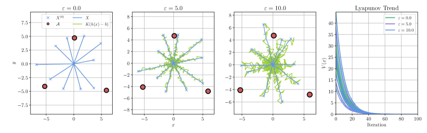
Figure 2: Response of the distance-coupled controller (13) with $x^{(\text{eq})}$ at the origin and for varying magnitudes of randomly generated measurement noise, $\omega_{\varepsilon}$. The agents are given arbitrary initial positions around the origin.

Let us now study the case when the set $\mathcal{A}$ is transformed by some orthogonal rotation, $R\in\mathbb{R}^{n\times n}$, and offset $r\in\mathbb{R}^{n}$, but the distance-coupled controller components (11) remain constant. That is, $\tilde{a}_{i}\in\mathbb{A}$ are the coordinates which were originally used to derive (11), where $\mathbb{A}$ is referred to as the anchor frame. The true positions are denoted $a_{i}\in\mathbb{W}$, where $\mathbb{W}$ is the world frame.

For a given anchor we can thus define the transformation

$$a_{i}=R\tilde{a}_{i}+r:\tilde{a}_{i}\in\mathcal{A}.$$ (17)

We differentiate between the two frames as the transformation of the set $\mathcal{A}$ creates error in the agent position defined by (12). That is,

$$\tilde{x} =K(h(x)-b)=R^{\intercal}(x-r),$$ (18)

where $x\in\mathbb{W}$ represents the world frame position of the agent and $\tilde{x}\in\mathbb{A}$ is its approximation in the anchor frame. The distance-coupled control function similarly becomes

$$\tilde{u}(x) =C(K(h(x)-b)-x^{(\text{eq})})$$ (19)

$$=C(\tilde{x}-x^{(\text{eq})})=C(R^{\intercal}(x-r)-x^{(\text{eq})})$$

$$=R^{\intercal}C(x-(Rx^{(\text{eq})}+r))$$

Likewise to Proposition 1, we can prove stability in terms of a range of acceptable values for the rotation and offset of the anchors. In order to make concrete claims on the stability of a system in $\mathbb{R}^{2}$, we identify the range of acceptable $\theta$ which make $R$ positive definite. This finding will be subsequently used in Proposition 2.

Lemma 1:

A 2-D rotation defined by $R(\theta)\in\mathbb{R}^{2\times 2}:\theta\in\mathbb{R}$ is positive definite for the range $\theta\in(2\pi k-\tfrac{\pi}{2},2\pi k+\tfrac{\pi}{2})$ $\forall k\in\mathbb{Z}$ where $\mathbb{Z}$ is the set of integers.

Proof.

Define the matrix $R$ in terms of Rodrigues’ formula for 2-D rotations:

$$R(\theta)=\begin{bmatrix}\cos(\theta)&-\sin(\theta)\\ \sin(\theta)&\cos(\theta)\end{bmatrix}$$ (20)

where $\theta$ is some scalar angle. For some arbitrary point, $x$, we can say $R\succ 0$ when $x^{\intercal}Rx>0$ for all $x\neq 0$. Expanding this condition we get that

$$x^{\intercal}Rx =[x_{1}\ x_{2}]\begin{bmatrix}\cos(\theta)&-\sin(\theta)\\ \sin(\theta)&\cos(\theta)\end{bmatrix}\begin{bmatrix}x_{1}\\ x_{2}\end{bmatrix}>0$$ (21)

$$=(x_{1}^{2}+x_{2}^{2})\cos(\theta)>0,$$

letting us conclude that $R(\theta)$ is positive definite so long as $\cos(\theta)>0$. This is true for the ranges

$$\theta\in(2\pi k-\tfrac{\pi}{2},2\pi k+\tfrac{\pi}{2})\ \forall k\in\mathbb{Z},$$ (22)

where $\mathbb{Z}$ is the set of integers.

By this, the stability candidate developed in Proposition 1 can be reformulated for the rotated anchor case and used to identify the region of attraction for (19).

Proposition 2:

For a 2-D system where the set $\mathcal{A}$ has been transformed by an orthogonal rotation, $R$, and translation, $r$, the distance-coupled controller (19) describes an exponentially stable policy with equilibrium $x=Rx^{(\text{eq})}+r$ for any $r$ and any $R$ given that $R^{\intercal}C\prec 0$ where $C$ is defined in Proposition 1 and $R$ in Lemma 1.

Proof.

Start by assuming that the new equilibrium, $\tilde{x}^{(\text{eq})}\in\mathbb{R}^{2}$, takes an equivalent transformation as that defined over the set $\mathcal{A}$, making the new Lyapunov candidate:

$$V(x) =(x-\tilde{x}^{(\text{eq})})^{\intercal}(x-\tilde{x}^{(\text{eq})})$$ (23)

$$=(x-(Rx^{(\text{eq})}+r))^{\intercal}(x-(Rx^{(\text{eq})}+r)).$$

We thus have $V(x)=0:x=\tilde{x}^{(\text{eq})}=Rx^{(\text{eq})}+r$ and $V(x)>0$ otherwise. Taking the derivative we get

$$\dot{V}(x) =2(x-(Rx^{(\text{eq})}+r))^{\intercal}\tilde{u}(x)$$ (24)

$$=2(x-(Rx^{(\text{eq})}+r))^{\intercal}C(K(h(x)-b)-x^{(\text{eq})}),$$

where $\tilde{u}(x)$ is the controller defined in (19). Thus giving

$$\dot{V}(x) =2(x-(Rx^{(\text{eq})}+r))^{\intercal}C(R^{\intercal}(x-r)-x^{(\text{eq})})$$ (25)

$$=2(x-(Rx^{(\text{eq})}+r))^{\intercal}R^{\intercal}C(x-(Rx^{(\text{eq})}+r)).$$

By inspection, we can conclude that $\dot{V}(x)=0:x=\tilde{x}^{(\text{eq})}=Rx^{(\text{eq})}+r$. Moreover, $\dot{V}(x)$ is negative definite so long as $R^{\intercal}C\prec 0$. If we assume $C\prec 0$ by Proposition 1, then, $R^{\intercal}C\prec 0$ if $R$ is defined as in Lemma 1.

Remark:

While Proposition 2 is limited to $\mathbb{R}^{2}$ for simplicity, we identify that, given $C\prec 0$, the final claim holds for any system in $\mathbb{R}^{n}$ given that $R$ is a positive definite orthogonal rotation in $\mathbb{R}^{n}$.

III-D Distance-coupled Homing Results

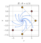
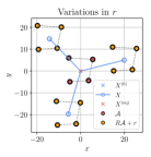
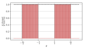
Figure 3: Homing controller response with $x^{(\text{eq})}=0$ and with variations in $R$ and $r$ simulated separately for $x^{(0)}$ chosen outside $Rx^{(\text{eq})}+r$.

Figure 4: Ratio of $100$ tests diverged for $100$ rotations, defined by $R:\theta\in[-2\pi,2\pi]$, of the anchor positions in $\mathcal{A}$.

We now validate the response of the distance-coupled controller (13) with varying degrees of noise in the measurement terms. The claims made on the regions of attraction defined in (22) will also be demonstrated. Note that the control coefficients are defined as $C=\alpha\mathbf{I}:\alpha=-5$ in all cases.

Let us define $\omega_{\varepsilon}$ as a uniformly distributed random variable with expected values in the range $[-\varepsilon,\varepsilon]$. The measurement noise is thus described as

$$d_{i}(x,\varepsilon)=d_{i}(x)+\omega_{\varepsilon}.$$

Figure 2 shows the response of the system with $p=3$ anchors and for varying degrees of noise, $\varepsilon$. The first case shows the ideal measurement scenario. That is, $\varepsilon=0$ with no error in the positions of the anchors. We place $x^{(\text{eq})}$ at the origin for simplicity. In this case, it is clear that there is no deviation between the true position and the anchor frame approximation. Likewise, the Lyapunov function converges ($V(x)\rightarrow 0$) as predicted from Proposition 1.

With an incorporation of a relatively large degree of measurement error ($\varepsilon=5$ and $\varepsilon=10$) we observe considerable differences between the approximation of the position from the distance-coupled function and the true position of the agent. Nonetheless, the agent is still capable of converging to a region around the equilibrium from any point.

Next, we validate the claims made in Section III-C for transformations of the anchors without updating (11). We first define the rotation $R:\theta=\tfrac{\pi}{4}$ and show that the agents converge with a policy defined by $R^{\intercal}C$. In the translation case, we sample various $r$ as uniform translations of the anchor set. Both sets of results are shown in Figure 4.

To demonstrate the region of attraction with respect to the rotation, $R$, of the anchors we can look at the behavior of the system for various angles $\theta$. Figure 4 shows the divergence rate for an agent with initial conditions

$$x^{(0)}=x^{(\text{eq})}+\omega_{\varepsilon},$$

where $\varepsilon=0.001$ is intentionally selected to be very small. We then show the results for $100$ uniformly spaced $\theta\in[-2\pi,2\pi]$ which were simulated until the candidate function converged ($V(x)\rightarrow 0$) or diverged ($V(x)\rightarrow\infty$). Each value in Figure 4 is the result of $100$ initial conditions. The system clearly stabilizes for all $\theta$ defined by the bounds in (22), and diverges otherwise. For a more explicit example, Figure 5 shows a series of agents initialized with $\omega_{\varepsilon=2.5}$ and $R:\theta=\tfrac{3\pi}{4}$ diverging from the origin as expected from (22).

IV Distance-coupled Formation Control

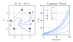
Figure 5: Distance-coupled controller response with the rotation, $R:\theta=\tfrac{3\pi}{4}$, of the anchor set (controller diverges).

Using the distance-coupled homing controller (13), we will define a new policy which drives $m$-agents to some predetermined formation. The only measurements each agent can make is the Euclidean distance it stands from each of the other agents in the environment. The following sections discuss the new system’s structure, defines the distance-coupled formation controller and proves certain properties analytically before demonstrating said claims in simulation.

IV-A Distance-coupled Formation Control

We utilize $m=p$ agents, with positions denoted by (3) and an intended formation described by the set $\mathcal{A}$. By defining our formation in terms of $\mathcal{A}$ we can exploit the notation from (12) to approximate the position of the agents in the anchor frame (discussed in Section IV-B).

In this scenario, each agent acts as an anchor for the others and vice versa. Thus, for an agent, $x_{k}$, we have the agent-distance set, $\mathcal{D}(x_{k},X)$, which is defined similarly to (6). We note that, in this form, the $k$-th element of the agent-distance set is always equal to $0$.

We define the corresponding list of desired positions as

$$X^{(\text{eq})}=\begin{bmatrix}x^{(\text{eq})}_{1}&\cdots&x^{(\text{eq})}_{m}\end{bmatrix}=\text{hstack}(\mathcal{A}),$$ (26)

where hstack$(\cdot)$ is the horizontal alternative to vstack$(\cdot)$. In order to utilize (12) for all agents, we expand the measurement vector from (11) to the matrix:

$$H(X)=\begin{bmatrix}h(x_{1})&\cdots&h(x_{m})\end{bmatrix},$$ (27)

where $h(x_{k})$ is the distance-coupled agent measurements derived from $\mathcal{D}(x_{k},X)$, i.e.

$$h(x_{k})=\text{vstack}(\{d^{2}(x_{k},x_{i})-d^{2}(x_{k},x_{j}):\forall(i,j)\in\mathcal{I}\}).$$ (28)

We similarly arrange the squared anchor difference vector from (11) as

$$B=b\mathbf{1}_{m}^{\intercal},$$ (29)

where $\mathbf{1}_{m}\in\mathbb{R}^{m}$ is a vector of all ones. This is valid as the vector $b$ is equivalent for every agent in $X$. Using the matrix notations defined above we can reformulate (12) and (13) as

$$X=K(H(X)-B),$$ (30)

$$U(X)=C(K(H(X)-B)-X^{(\text{eq})}),$$ (31)

where $K$ is similarly unchanged from (12). Finally, we can note that the only parameter which differs between the agents is the intended equilibrium position, identified by $x^{(\text{eq})}_{k}$ in the matrix $X^{(\text{eq})}$.

IV-B Formation Equivalence in the Anchor Frame

Before further inspection, we define formation equivalence (or, congruence) between the two frames of reference, $\mathbb{A}$ and $\mathbb{W}$, using selected tools from Procustes analysis [15]. Similar to the offsets defined in Section III-C, we have the agent positions in the world frame, $X\in\mathbb{W}$, with corresponding anchor frame coordinates $\tilde{X}\in\mathbb{A}$.

Definition 1:

Procrustes analysis defines the two sets, $X$ and $\tilde{X}$, as congruent if

$$\exists\Psi\text{ s.t. }X-\langle x\rangle=\Psi(\tilde{X}-\langle\tilde{x}\rangle),$$ (32)

given the orthogonal rotation, $\Psi(X,\tilde{X})=R(\theta)$, and the centroid of the formation, $\langle x\rangle=\tfrac{1}{m}\Sigma_{k=1}^{m}x_{k}$.

In practice, we can calculate an approximation of $\Psi$ using the Kabsch algorithm [16]. The resulting matrix is the most optimal rotation which superposes the set $\tilde{X}$ onto $X$.

Another method of denoting the transformation (32) is to combine the constant terms on the left and right sides into a single linear translation which superposes the anchor frame formation onto the world frame. This turns (32) into

$$X-\langle x\rangle=\Psi(\tilde{X}-\langle\tilde{x}\rangle)\;\Rightarrow\;X=\Psi\tilde{X}+\psi,$$ (33)

where $\psi=\langle x\rangle-\Psi\langle\tilde{x}\rangle$. The later sections will primarily use the shorthand definition of formation error (33). It can be further noted that the uniform scaling component to Procrustes analysis is omitted.

In order to measure policy convergence in Section IV-E, we define the formation error between $X$ and $X^{(\text{eq})}$ as the $L_{2}$-norm of the function (33) on individual agents, i.e.

$$W(X)=\Sigma_{k=1}^{m}\|(\Psi x_{k}+\psi-x^{(\text{eq})}_{k})\|_{2}.$$ (34)

IV-C Transformation Invariance

In order to discuss the equilibria of (31) we define transformation invariance and prove its application to the distance function. These claims will be used to similarly prove the invariance of (30) and (31) in the next section.

Definition 2:

A function $f(x,y):x,y\in\mathbb{R}^{n}$ is transformation invariant if $f(x,y)$ is constant under equivalent rotations and translations of both $x$ and $y$. That is,

$$f(Rx+r,Ry+r)=f(x,y),$$ (35)

given that $R\in\mathbb{R}^{n\times n}$ is an orthogonal rotation and $r\in\mathbb{R}^{n}$.

Lemma 2:

The distance function,

$$d(x,y)=\sqrt{(x-y)^{\intercal}(x-y)},$$ (36)

is transformation invariant by Definition 2.

Proof.

Define an arbitrary orthogonal rotation, $R$, and translation, $r$, of the original states $x$ and $y$ such that

$$x\rightarrow Rx+r\text{, and }y\rightarrow Ry+r.$$ (37)

Taking the distance between the transformed points:

$$d(Rx+r,Ry+r)=\\ \sqrt{(Rx+r-(Ry+r))^{\intercal}(Rx+r-(Ry+r))}\\ \begin{aligned} &=\sqrt{(x-y)^{\intercal}R^{\intercal}R(x-y)}\\ &=\sqrt{(x-y)^{\intercal}(x-y)},\end{aligned}$$

which is equivalent to (36). Thus concluding that the distance function follows by Definition 2.

IV-D Equilibria of the Distance-coupled Formation Controller

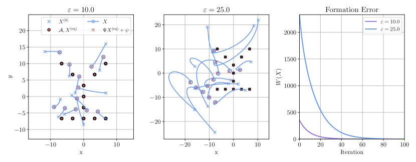
Figure 6: Distance-coupled formation control response for an arbitrary formation pattern and with varying levels of randomly generated offsets from the equilibrium positions: $X^{(0)}=X^{(\text{eq})}+\omega_{\varepsilon}$.

Using Lemma 2 we establish the invariance of the distance-coupled functions in $H(X)$. Subsequently, we will use this claim to derive the equilibria of (31).

Proposition 3:

The distance-coupled position (30) is transformation invariant for any congruent set of positions $X=\Psi\tilde{X}+\psi$.

Proof.

Let there exists an orthogonal rotation $\Psi$ and translation $\psi$ so that $X$ and $\tilde{X}$ are congruent. Identifying that the dependent variables in (30) are solely contained in $H(X)$, we isolate a single row of the measurement terms for an arbitrary agent, $h(x_{k})$. That is,

$$h_{i,j}(x_{k})=d^{2}(x_{k},x_{i})-d^{2}(x_{k},x_{j}),$$ (38)

for given indices $(i,j)$. Applying the transformation $(\Psi,\psi)$ to the entire formation, we get

$$h_{i,j}(\Psi\tilde{x}_{k}+\psi)=d^{2}(\Psi \tilde{x}_{k}+\psi,\Psi\tilde{x}_{i}+\psi)$$ (39)

$$-d^{2}(\Psi\tilde{x}_{k}+\psi,\Psi\tilde{x}_{j}+\psi).$$

Identifying the transformation invariance of the distance function from Lemma 2:

$$h_{i,j}(\Psi\tilde{x}_{k}+\psi) =d^{2}(\tilde{x}_{k},\tilde{x}_{i})-d^{2}(\tilde{x}_{k},\tilde{x}_{j})$$ (40)

$$=h_{i,j}(\tilde{x}_{k}).$$

Therefore, for a transformation on the entire agent group, (40) holds for all $(i,j)\in\mathcal{I}$ and for any agent, $x_{k}$. This implies that every element in the measurement matrix, $H(X)$, is also transformation invariant. Combining this with the position given by (30), we get that

$$H(X)=H(\Psi\tilde{X}+\psi)=H(\tilde{X})$$ (41)

$$\begin{aligned} \Rightarrow K(H(X)-B)&=K(H(\Psi\tilde{X}+\psi)-B)\\ &=K(H(\tilde{X})-B)=\tilde{X}.\end{aligned}$$

Proving that (30) is transformation invariant.

Proposition 4:

The controller (31) is transformation invariant for any congruent $X$ and $\tilde{X}$.

Proof.

Let us assume that Proposition 3 is true for the rotation $\Psi$ and translation $\psi$. Then we have that

$$U(X) =C(K(H(\Psi\tilde{X}+\psi)-B)-X^{(\text{eq})})$$ (42)

$$=C(K(H(\tilde{X})-B)-X^{(\text{eq})})$$

$$=U(\tilde{X}).$$

Implying that (31) is transformation invariant for any congruent $X$ and $\tilde{X}$.

We can then use Proposition 4 to identify the equilibria of the distance-coupled formation controller.

Corollary 1:

The formation controller (31) is at an equilibrium, $U(X)=0$, for any $X$ which is congruent to $\tilde{X}=X^{(\text{eq})}$.

Proof.

Assume that $\tilde{X}=X^{(\text{eq})}$ such that $U(\tilde{X})=0$. Then, for the world frame positions, $X=\Psi\tilde{X}+\psi$, and by Proposition 4 we have that

$$U(X)=U(\Psi\tilde{X}+\psi)=U(\tilde{X})=U(X^{(\text{eq})})=0.$$ (43)

Proving that the positions $X$ are at an equilibrium given they are congruent to $\tilde{X}$.

It should be noted that, while Corollary 1 defines the equilibria of (31), it makes no claims on its stability. However, because of the similarities between (13) and (31), it can be reasonably deduced that, for agent positions $X$ which are not congruent to $\tilde{X}$, we get similar bounds on the region of attraction as those shown in (22). This is demonstrated in the results for small perturbations of the agents from the equilibrium for various rotations.

IV-E Distance-coupled Formation Results

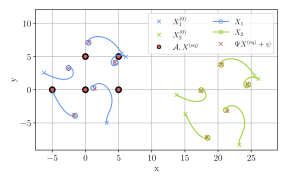
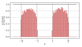
Figure 7: Response of formation controller with offset $\omega_{\varepsilon=10}$ and for the two agent sets with positions denoted by $X_{2}=X_{1}+r$.

Figure 8: Region of attraction results with $p=4$ and $100$ repetitions at each $R:\theta\in[-2\pi,2\pi]$ for a randomly generated offset with $\omega_{\varepsilon=0.1}$.

While we do not present a proof for the stability of the distance-coupled formation controller, we can demonstrate empirically its behavior under various initial conditions. We first show the response of the policy when the initial conditions are randomly offset around $X^{(\text{eq})}$. This will also help to validate our claims on the equilibrium positions defined in Corollary 1. The region of attraction will then be plotted similarly to Figure 4, and the results will be compared.

To validate the response of (31) we initialize the agent group such that

$$X^{(0)}=X^{(\text{eq})}+\omega_{\varepsilon},$$

with $\varepsilon=10$ and $\varepsilon=25$. The simulation is then iterated and the behavior of the policy is shown. The performance of the formation error function $W(X)$ is plotted over time for each test, showing that it converges in these two cases.

Figure 8 uses two sets of agents to validate the convergence of the formation controller for similarly perturbed formations. The first set, $X_{1}$, is the reference set and has initial conditions which are generated similar to the Figure 6 example with $\varepsilon=10$. The second set is linearly offset from $X_{1}$ by a constant $r$. As expected, the two sets follow the same trajectory and end in equilibrium positions which differ by the initial translation, $r$.

Because of their close relationship, we tested if the controller would behave similarly to rotations about the origin as it does in the homing problem. We thus modified the initial condition formula for the agent set such that

$$X^{(0)}=R(X^{(\text{eq})}+\omega_{\varepsilon}),$$

with $\varepsilon=0.1$ and for the same list of $\theta$ described in Section III-D. The simulation was then iterated until the controller converged ($W(X)\rightarrow 0$) or diverged ($W(X)\rightarrow\infty$), and the proportion of tests which diverged for $100$ samples are shown in Figure 8. As expected, there is a strong correlation to the bounds defined in (22), with more complicated interplay in the formation policy case. Figure 9 shows an example of the controller diverging with $R:\theta=\pi$ and $\omega_{\varepsilon=0.1}$.

V Conclusion

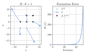
Figure 9: Divergence of (31) with initial conditions $x^{(0)}=Rx^{(\text{eq})}$ given $R:\theta=\pi$ and $\omega_{\varepsilon=0.1}$.

In this paper we define the distance-coupling method as a suitable approach to the position and formation control problems. In the homing case we prove stability and show that it is held for linear transformations of the anchor positions, even when the policy components (11) are not updated. The distance-coupled formation controller is also studied, and the equilibrium conditions are established under the definitions of congruence and transformation invariance. Claims are made on the general performance of the system under arbitrary transformations, and the resulting convergence properties are demonstrated empirically.

Generally speaking, the approach described here is framed using a single-integrator model (1) for simplicity. That said, the distance-coupled position functions (12) and (30) can be applied to any localization problem in which the available measurements are a function of the distance from known reference points. In the context of systems with more complex dynamics, the distance-coupled policies defined here can be used to calculate suitable waypoints for the agents to follow by a more appropriate controller.

References

- [1] Michael S. Floater “Generalized barycentric coordinates and applications” Publisher: Cambridge University Press In Acta Numerica 24, 2015, pp. 161–214 DOI: 10.1017/S0962492914000129
- [2] Kaveh Fathian et al. “Distributed Formation Control via Mixed Barycentric Coordinate and Distance-Based Approach” ISSN: 2378-5861 In 2019 American Control Conference (ACC), 2019, pp. 51–58 DOI: 10.23919/ACC.2019.8814890
- [3] Tingrui Han, Zhiyun Lin, Ronghao Zheng and Minyue Fu “A Barycentric Coordinate-Based Approach to Formation Control Under Directed and Switching Sensing Graphs” Conference Name: IEEE Transactions on Cybernetics In IEEE Transactions on Cybernetics 48.4, 2018, pp. 1202–1215 DOI: 10.1109/TCYB.2017.2684461
- [4] Dimos V. Dimarogonas and Kostas J. Kyriakopoulos “A connection between formation infeasibility and velocity alignment in kinematic multi-agent systems” In Automatica 44.10, 2008, pp. 2648–2654 DOI: 10.1016/j.automatica.2008.03.013
- [5] Dimos V. Dimarogonas, Panagiotis Tsiotras and Kostas J. Kyriakopoulos “Leader–follower cooperative attitude control of multiple rigid bodies” In Systems & Control Letters 58.6, 2009, pp. 429–435 DOI: 10.1016/j.sysconle.2009.02.002
- [6] Zhiyun Lin, B. Francis and M. Maggiore “Necessary and sufficient graphical conditions for formation control of unicycles” Conference Name: IEEE Transactions on Automatic Control In IEEE Transactions on Automatic Control 50.1, 2005, pp. 121–127 DOI: 10.1109/TAC.2004.841121
- [7] Dimos V. Dimarogonas and Karl H. Johansson “On the stability of distance-based formation control” ISSN: 0191-2216 In 2008 47th IEEE Conference on Decision and Control, 2008, pp. 1200–1205 DOI: 10.1109/CDC.2008.4739215
- [8] Yun Ho Choi and Doik Kim “Distance-Based Formation Control With Goal Assignment for Global Asymptotic Stability of Multi-Robot Systems” Conference Name: IEEE Robotics and Automation Letters In IEEE Robotics and Automation Letters 6.2, 2021, pp. 2020–2027 DOI: 10.1109/LRA.2021.3061071
- [9] J. Baillieul and A. Suri “Information patterns and Hedging Brockett’s theorem in controlling vehicle formations” In Proceedings of the 42nd IEEE, 2003 URL: https://ieeexplore.ieee.org/document/1272622
- [10] Wei Ren and Ella Atkins “Distributed multi-vehicle coordinated control via local information exchange” _eprint: https://onlinelibrary.wiley.com/doi/pdf/10.1002/rnc.1147 In International Journal of Robust and Nonlinear Control 17.10-11, 2007, pp. 1002–1033 DOI: 10.1002/rnc.1147
- [11] Ting Chen et al. “Formation control for second-order nonlinear multi-agent systems with external disturbances via adaptive method” ISSN: 2688-0938 In 2022 China Automation Congress (CAC), 2022, pp. 5616–5620 DOI: 10.1109/CAC57257.2022.10055393
- [12] Zhiyun Lin, Lili Wang, Zhimin Han and Minyue Fu “Distributed Formation Control of Multi-Agent Systems Using Complex Laplacian” In IEEE Transactions on Automatic Control 59.7, 2014, pp. 1765–1777 DOI: 10.1109/TAC.2014.2309031
- [13] Kwang-Kyo Oh, Myoung-Chul Park and Hyo-Sung Ahn “A survey of multi-agent formation control” In Automatica 53, 2015, pp. 424–440 DOI: 10.1016/j.automatica.2014.10.022
- [14] Hassan Khalil “Nonlinear Systems” Pearson, 2001 URL: https://www.pearson.com/en-us/subject-catalog/p/nonlinear-systems/P200000003306/9780130673893
- [15] Mikkel B Stegmann and David Delgado Gomez “A Brief Introduction to Statistical Shape Analysis”
- [16] W. Kabsch “A discussion of the solution for the best rotation to relate two sets of vectors” Number: 5 Publisher: International Union of Crystallography In Acta Crystallographica Section A: Crystal Physics, Diffraction, Theoretical and General Crystallography 34.5, 1978, pp. 827–828 DOI: 10.1107/S0567739478001680