SLO/GO Degradation–Loss Sensitivity in Climate–Human System Coupling

Abstract

The potential of extreme environmental change driven by a destabilized climate system is an alarming prospect for humanity. But the intricate, subtle ways Earth’s climate couples to social and economic systems raise the question of when more incremental climate change signals the need for alarm. Questions about incremental sensitivity are particularly crucial for human systems that are organized by optimization. Optimization is most valuable in resolving complex interactions among multiple factors, however, those interactions can obscure coupling to underlying drivers such as environmental degradation. Here, using Multi-Objective Land Allocation as an example, we show that model features that are common across non-convex optimization problems drive hypersensitivities in climate-induced degradation–loss response. We show that catastrophic losses in human systems can occur well before catastrophic climate collapse. We find punctuated insensitive/hypersensitive degradation–loss response, which we trace to the contrasting effects of environmental degradation on subleading, local versus global optima (SLO/GO). We argue that the SLO/GO response we identify in land-allocation problems traces to features that are common across non-convex optimization problems more broadly. Given the broad range of human systems that rely on non-convex optimization, our results therefore suggest that substantial social and economic risks could be lurking in a broad range in human systems that are coupled to the environment, even in the absence of catastrophic changes to the environment itself.

I Introduction

Climate change investigations [1] indicate that destabilizing Earth’s climate system may drive extreme environmental shifts that harbour catastrophic impacts on humanity. However, the coupling of human social and economic organization to the climate is complex [2], so the sensitivity of a given form of human organization to climate change is unclear.[2] For example, will large-scale changes in how we organize our societies and economies only stem from widespread environmental catastrophe? Or, could the nature of human–climate coupling drive large-scale changes in human organization in response to minor climate change? Understanding these questions is critical as data show Earth’s climate continues to warm [3].

Parameter sensitivity questions are crucial for land-use planning. Environmental changes, such as increased flood risk [4], reductions in precipitation [5] or a decline in soil quality [6], change the suitability of land for specific uses. These changes have knock-on social and economic impacts, such as via insurance costs [7] or crop yields [3], among other factors. Moreover, even rapid land redevelopment or rehabilitation occurs on significant timescales.[8] If small changes in climate conditions can trigger large-scale redistribution of optimal land-use patterns, the mismatch in timescales between the redistribution trigger and the land-use re-development response could create social and economic instability. Understanding land-use decision making methods’ resilience to climate change therefore provides an important set of test cases for studying the relationship between sensitivity and risk. In particular, land-use planning procedures can invoke non-convex optimization techniques. Therefore, the way in which non-convexity drives land-use planning responses to environmental degradation could signal the existence of analogous effects in other systems of human organization.

Here, using a model [9] from the literature on geographic information systems (GIS) informed land-use planning [10], we show that land-use planning exhibits punctuated hypersensitivity to climate change, in which marginal land degradation can drive large-scale land reallocation. Via a bespoke Markov Chain Monte Carlo (MCMC) sampling implementation in C++ [11] we frame the results of $1.2\times 10^{6}$ statistically independent planning simulations in terms of a degradation–loss ($\Delta$–$\Lambda$) framework. Our computed $\Delta$–$\Lambda$ response reveals that marginal changes in land suitability produce hypersensitive land-use response. We find that the non-linear coupling between land allocation and degradation results in the complete loss of specific land uses that occurs well before complete degradation. We give a schematic representation of our approach in Fig. 1

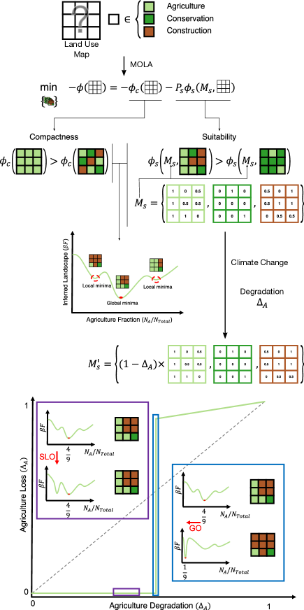
Figure 1: Schematic illustration of model of climate change-induced environmental degradation in land allocation. Multi-Objective Land Allocation (MOLA) supports land-use planning by casting the problem of determining land-use maps (here for simplicity we illustrate this via $3\times 3$ maps) as a weighted optimization problem. Typical planning criteria invoke notions of spatial compactness and land suitability, but optimal overall outcomes are typically not optimal for either component criterion, but instead involve complex trade-offs, and these trade-offs make it difficult to anticipate how planning would be affected by effects of climate change. We model this by incorporating potential future degradation in suitability for agricultural use. We compute the resulting loss of agricultural land under optimal scenarios in the face of degradation.

To understand the origin and generality of these effects, we use brute force methods to infer the parametric dependence of the landscapes of the underlying non-convex optimization problem. We trace the origin of punctuated insensitive/hypersensitive response to the non-uniform effect that environmental degradation has on the underlying optimization landscape of the coupled human system. It would be intuitive to expect that insensitive response occurs when degradation has only a minor effect on the optimization landscape. We find, instead, that degradation insensitivity can co-occur with large changes in optimization landscapes if landscape changes are primarily concentrated among sub-leading, local optima (SLO). In contrast to SLO-associated, insensitive degradation response we find that hypersensitive response occurs when changes in the optimization landscape affect global optima (GO).

Our analysis reveals two alarming outcomes: (i) that land-use planning models exhibit hypersensitivity to marginal climate change, and (ii) that, in all test cases, total loss greatly preceded total degradation. Additionally, our analysis indicates that the punctuated insensitive/hypersensitive response we observed was driven by systems with non-uniform, SLO/GO, parametric dependence across the optimization landscape. The fact that this phenomenon can be traced to such a generic feature of non-convex optimization is concerning because non-convex optimization problems support social and economic organization in a wide range of sectors such as airline networks,[12] food harvesting,[13] energy distribution,[14] among others. The generic mechanism that drives our findings thus signals that the SLO/GO induced hypersensitivities we observed here could have alarming analogues in a broad range of other areas of human activity. It is therefore vital to extend the degradation–loss framework we presented here to identify and mitigate brewing catastrophes that minor environmental change could induce in other sectors of human social and economic activity.

II Results

II.1 Partial Degradation Drives Total Loss

To determine the effect of climate change-induced degradation on land-use distributions, we sampled land-use patterns from $1.2\times 10^{6}$ statistically independent MCMC simulations of a set of MOLA models (see Methods). A MOLA model typically includes planning priorities of spatial compactness and land suitability for a given set of uses, encoded as numerical factors [10]. We used a reduction in the land-suitability factor to model the effect of climate change via a degradation factor $\Delta_{A}$ assigned to agriculture that ranged between $0$ (no degradation) and $1$ (complete degradation). We extracted optimal land-use patterns from sampled configurations, and computed agriculture loss $\Lambda_{A}$, the fractional reduction in land-use for agriculture, between $0$ (no loss compared to coverage at $\Delta_{A}=0$) and $1$ (complete loss compared to coverage at $\Delta_{A}=0$).

MOLA outcomes depend strongly on the relative prioritization of planning objectives. A prior investigation of the current model without degradation [15] showed that significant compactness–suitability trade-offs occur when the relative priority, parameterized via a so-called suitability pressure $P_{S}$, falls in the range $(0,8)$. We selected six different values of $P_{S}$ to ensure that our analysis addresses distinct trade-off regimes previously found in Ref. [15] in the absence of degradation. $\Delta$–$\Lambda$ response for six trade-off regimes is shown in Fig. 2.

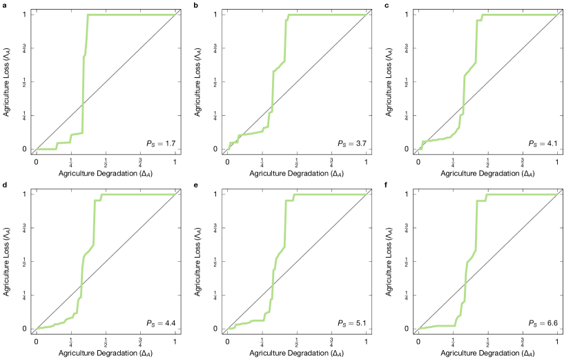
Figure 2: Degradation–Loss ($\Delta$–$\Lambda$) response of climate-coupled Multi-Objective Land Allocation (MOLA) shows that moderate degradation induces total loss and that marginal degradation produces punctuated insensitive/hypersensitive response. Panels a-f show $\Delta$–$\Lambda$ response in six compactness–suitability trade-off regimes. Results are for uniform relative agricultural degradation $\Delta_{A}$ where 0 represents no degradation, and 1 represents total degradation. Vertical axes represent relative land-use loss $\Lambda_{A}$. $\Lambda_{A}$ is normalized so that baseline land use coverage is taken relative to zero degradation (i.e. $\Lambda_{A}(\Delta_{A}=0)\equiv 0$) and total loss corresponds to $\Lambda_{A}=1$. $P_{S}$ values (inset) parameterize the relative weight of suitability relative to compactness in the model. $P_{S}$ values are selected to fall in compactness/suitability trade-off regimes identified in a prior, zero degradation investigation. In all cases $\Lambda_{A}=1$ for $\Delta_{A}<\tfrac{1}{2}$ indicating that moderate environmental degradation induces total land use loss. Additionally, the jagged, step-wise form of the response curves indicates that all cases exhibit punctuated insensitive/hypersensitive $\Delta$–$\Lambda$ response.

$\Delta$–$\Lambda$ response in Fig. 2 indicates that in all studied cases, the onset of total loss $\Lambda_{A}=1$, occurs well before the advent of total degradation, $\Delta_{A}=1$. Indeed, we find that in all cases we studied $\Lambda_{A}\to 1$ for $\Delta_{A}<\tfrac{1}{2}$. The finding that partial degradation drives total loss is concerning because it indicates that as climate change-induced environmental degradation feeds into a human system organized by non-convex optimization, even moderate degradation can lead to potentially catastrophic changes in land-use patterns.

II.2 Punctuated Insensitive/Hypersensitive Degradation–Loss Response

We next examine the degradation–loss ($\Delta$–$\Lambda$) response before the onset of total loss. This is also shown in Fig. 2 and corresponds to a portion of the $\Delta$–$\Lambda$ response curve that falls to the left of the onset of total loss. In all six compactness–suitability trade-off regimes we studied, we find that the $\Delta$–$\Lambda$ response is characterized by a series of step-wise increases in loss. This step-wise form signals that agricultural land-use loss ($\Lambda_{A}$) has a punctuated insensitive/hypersensitive dependence on the degree of agriculture degradation ($\Delta_{A}$).

A better understanding of how $\Delta$–$\Lambda$ data support this interpretation requires comparing with general expectation. In general $\Delta$–$\Lambda$ response should pass through the points $(0,0)$ and $(1,1)$, i.e., we define loss relative to a baseline land-use fraction at zero degradation, and we expect that complete degradation will lead to complete loss. The fragility or resilience of the $\Delta$–$\Lambda$ response is determined by how the system responds between these extremes. The grey line in each plot gives the response of a hypothetical system that exhibits a linear response that is commensurate with expectations for zero and complete loss. With this framing, it is possible to use $\Delta$–$\Lambda$ plots to identify both overall- and marginal sensitivity. Low overall sensitivity can be identified as the degree to which $\Delta$–$\Lambda$ response falls in the range $\Lambda<\Delta$ (i.e., overall relative degradation exceeds overall relative loss). Conversely, high overall sensitivity can be identified as the degree to which $\Delta$–$\Lambda$ response falls in the range $\Lambda>\Delta$ (i.e., overall relative loss exceeds overall relative degradation). Low sensitivity $\Lambda<\Delta$ indicates resilient climate–human system coupling that suppresses degradation effects. In contrast $\Lambda>\Delta$ indicates fragile climate–human system coupling that exacerbates degradation effects. Similarly, for marginal $\Delta$–$\Lambda$ sensitivity, “flat” (i.e. $d\Lambda/d\Delta\approx 0$) marginal response signals low sensitivity, which indicates marginal stability or resilience. In contrast “vertical” (i.e. $d\Lambda/d\Delta\to\infty$) marginal response signals hypersensitivity, which indicates marginal instability or fragility. Moderate sensitivity falls between these extremes.

Using the above lens for interpreting sensitivity, what we observed in Fig. 2 is not indicative of moderation. Instead, in all cases we observe that $\Delta$–$\Lambda$ response exhibits periods of low sensitivity, in which increasing $\Delta_{A}$ results in little to no change in $\Lambda_{A}$, punctuated by instances of hypersensitive response in which small changes in $\Delta_{A}$ produce very large changes in $\Lambda_{A}$. Our results indicate that the overall response appears resilient up to $\Delta_{A}\sim 0.3$ (with some $P_{S}$-dependent variation), after which there are a series of hypersensitivities that render the overall response largely fragile.

Taken together, our results indicate that marginal increases in degradation can induce large-scale losses, and that complete collapse of the land-use planning system can occur long before the complete degradation of the underlying climate system it is coupled to.

II.3 SLO/GO Landscape Rearrangement Drives Punctuated Hypersensitive Response

To understand the scope of these observations, it is instructive to identify their origin, which must trace back to the structure of the landscape of the underlying optimization problem. Fig. 3a shows the optimal land use fraction for all land uses as a function of $\Delta_{A}$ at fixed $P_{S}=4.4$ (see SI for other suitability pressures). To understand the origin of the difference between insensitive and hypersensitive response, we inferred underlying optimization landscapes from MCMC sampled allocation patterns. Key differences between insensitive and hypersensitive $\Delta$–$\Lambda$ response can be seen by comparing optimization landscapes for four values of degradation, $\Delta_{A}$, spaced by increments of 3% in Fig. 3b,c,d,e.

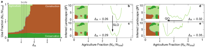
Figure 3: Changes in land-use patterns associated with hypersensitive degradation–loss ($\Delta$–$\Lambda$) response are driven by contrasts between subleading local optima (SLO) versus global optima (GO) rearrangements in underlying optimization landscapes. Panel a shows land-use distribution by degree of degradation shows punctuated insensitive/hypersensitive response in use patterns following $\Delta$–$\Lambda$ response shown in Fig. 1 (data are shown here for $P_{S}=4.4$, all other studied values of $P_{S}$ are shown in SI). This observed response arises from contrasting SLO/GO reorganization in the underlying landscapes. Panels b and c show use maps (inset) and inferred optimization landscapes at degradation amounts separated by 3% (b: $\Delta_{A}=0.26$; c: $\Delta_{A}=0.29$). The landscape plots show that this marginal increase in degradation results in minor changes in optimal land use patterns. However, this apparent insensitivity masks significant SLO rearrangement in inferred underlying optimization landscapes (see Methods). Panels d and e show use maps (inset) and inferred optimization landscapes at degradation amounts separated by 3% (d: $\Delta_{A}=0.32$; e: $\Delta_{A}=0.35$). Landscape plots show that this minor change in degradation affects underlying landscape’s GO organization, which is echoed by macroscopic rearrangement of the spatial land-use distribution.

Between degradation $\Delta_{A}=0.26$ (Fig. 3b) and $0.29$ (Fig. 3c) there is little change in the land-use fraction (Fig. 3a) and there is little change in the spatial distribution of land uses (inset maps in Fig. 3b,c). However, this marginal degradation-insensitivity in the optimal land pattern does not mean that there are no changes in the underlying optimization landscape. In fact, as a comparison between Fig. 3b and c shows, the optimization landscape reconfigures significantly between $\Delta_{A}=0.26$ and $0.29$, but the primary effect is on the sub-leading, local optimum (SLO).

As in Fig. 3b and c, the marginal increase in degradation between panels Fig. 3d and e is also 3%. However, the effect that increased degradation has on the land use fraction (Fig. 3a) and the spatial distribution land uses is dramatic. Comparing the underlying optimization landscapes at $\Delta_{A}=0.32$ (Fig. 3d) with that of $0.35$ (Fig. 3e) reveals that a relatively small increase in degradation affects the global optimum (GO), resulting in a reduction in the agricultural use fraction from $\approx 0.65$. to $\approx 0.38$. Normalized to a zero-degradation baseline, in this case a 3% change in degradation results in a relative loss of 32%.

Therefore, the punctuated nature of the response is caused by underlying optimization landscape rearrangement, with changes to SLO driving periods of insensitivity, and changes to GO producing hypersensitive response.

III Discussion

We modelled the effect of climate-change induced environmental degradation on land-use loss via multi-objective land allocation. Our degradation–loss analysis yielded two key outcomes. We found that the nature of the coupling of environmental degradation to a non-convex optimization model of land-use planning resulted in the onset of complete loss of land use well in advance of complete degradation of land-use suitability. Furthermore, we found that marginal increases at intermediate amounts of degradation produced punctuated insensitive/hypersensitive response in which increased degradation generally led to one of two outcomes: almost no losses in land use, or large amounts of loss. Moreover, we traced insensitive/hypersensitive response to reorganizations in the underlying optimization landscape that primarily affected the configuration of subleading, local optima (SLO) or the configuration of global optima (GO).

The SLO/GO-induced, punctuated insensitive/hypersensitive response we found here results from the differential effects of degradation on the form of the underlying landscape that originate, in turn, from the inhomogeneity of the land itself. Intrinsic spatial inhomogeneity gives rise to a set of local minima that respond unevenly to progressive environmental degradation. More formally, we observed that punctuated insensitive/hypersensitive response coincided with an optimization problem that had an optimization landscape with multiple local minima, and that these local minima had different parametric dependence on degradation. However, optimization landscapes with multiple local minima that have different parametric dependence are ubiquitous across non-convex optimization problems. The fact that a generic feature of non-convex optimization produces the SLO/GO behaviour that drives the punctuated insensitive/hypersensitive response we identified here suggests that a similar response could arise generically in situations where human systems are coupled to climate-induced environmental degradation.

The potential for the effects we observed to have analogues in other systems is concerning. Our investigation revealed that the effects of degradation can be easily masked in studies of human systems organized by optimization if the parametric dependence of the underlying landscape is not determined. The effects of degradation could then accumulate among subleading local minima, unnoticed, and drive subsequent hypersensitive response, seemingly without warning. I.e., in optimization settings, identifying weak marginal response to small amounts of environmental degradation provides no guarantee of subsequent stability.

Questions of stability are salient for, but not limited to, land-use. Triggering small, marginal environmental degradation could prompt response in the form of redevelopment and rehabilitation, human migration, or commercial and industrial relocation, all which occur over much longer timescales than the degradation. Other systems of social or economic organization could be imperilled by trigger/response timescale mismatches arising from SLO/GO-induced degradation–loss hypersensitivity if their dynamic response is limited by factors such as relocation, construction, manufacturing, procurement, deployment, or distribution. Worryingly, most social and economic systems that have a physical footprint are affected by multiple factors on that list. This suggests that SLO/GO features of optimization-based organization could prompt large-scale social and economic destabilization in many sectors even without large-scale destabilization of the climate itself. Given the importance of mitigating such instabilities, it would be valuable to extend the analysis given here, of elucidating the structure of the parametric dependence of the optimization landscape, to anticipate similar SLO/GO-induced instabilities in other human systems.

IV Methods

IV.1 Land Degradation Model

We employ a MOLA model from Ref. [16] that represents a 9 km² square area in the Xin’andu township of Dongxihu District, Wuhan, China [16] as a 30 by 30 grid. Each grid cell represents a parcel of land that can have one of three land use types: agriculture, construction, or conservation.

Land-use planning in such a setting can be informed by the use of weighted, multi-objective optimization based approaches to allocation. The model considered in Ref. [9] included spatial compactness and land suitability, two of the most widely used criteria [10] in optimal land-use allocation.

We aim to minimize an objective function that expresses the weighted combination of planning criteria, as suggested in Ref. [9],

$$\phi=-P_{C}\phi_{C}-P_{S}\phi_{S}\;.$$ (1)

In this equation, $P_{C}$ and $P_{S}$ are weights assigned to the objectives for compactness, $\phi_{C}$, and suitability, $\phi_{S}$ (explicit forms for $\phi_{C,S}$ are given below). $P_{C,S}$ can be interpreted as analogous to physical pressure [17]. The allocation’s characteristics are influenced by the relative values of $P_{C}$ and $P_{S}$. A predominance of one criterion over the other is seen when there is a significant disparity between $P_{C}\phi_{C}$ and $P_{S}\phi_{S}$. Conversely, a trade-off between the two criteria is achieved when $P_{C}\phi_{C}$ and $P_{S}\phi_{S}$ are of similar magnitudes.

The compactness criterion $\phi_{C}$ is given by

$$\phi_{c}=\sum_{k=0}^{K}\sum_{i=1}^{N}\sum_{j=1}^{M}c_{ijk}x_{ijk}\;.$$ (2)

Here, $M$ and $N$ index the map’s columns and rows, while $K$ denotes the number of distinct land-use types. The variable $x_{ijk}$ indicates whether the parcel at coordinates $(i,j)$ is designated for land-use type $k$, in which case $x_{ijk}=1$, otherwise it is $0$. The coefficient $c_{ijk}$ represents the number of matching neighbours for the parcel at $(i,j)$ and is defined as

$$c_{ijk}=x_{i+1j+1k}+x_{ij+1k}+x_{i+1jk}+x_{i-1jk}+x_{ij-1k}+x_{i-1j-1k}+x_{i-1j+1k}+x_{i+1j-1k}\;.$$ (3)

The suitability criterion $\phi_{S}$ is given by

$$\phi_{S}=\sum_{k=0}^{K}\sum_{i=1}^{N}\sum_{j=1}^{M}s_{ijk}x_{ijk};,$$ (4)

The suitability coefficient, $s_{ijk}$, quantifies the suitability of the parcel at $(i,j)$ for a specific land-use type $k$. We consider a $30\times 30$ map as per Ref. [9], with $M=N=30$, and three land-use types: agriculture, construction, and conservation, represented by $k=0,1,2$. Suitability data $s_{ijk}$ are detailed in the Supplementary Information (SI).

We investigated the trade-off regimes identified in Ref. [15] in a modified form of the model where we modelled climate-induced environmental degradation as a spatially-uniform scaling by a coefficient $\Delta_{A}$ of the land-use suitability for agriculture. We parameterized degradation between $\Delta_{A}=0$, zero degradation (baseline case), and $\Delta_{A}=1$ (total degradation). Mathematically, the suitability coefficient for agriculture, $k=0$, is scaled by $1-\Delta_{A}$ factor as

$$s^{\prime}_{ij0}=(1-\Delta_{A})s_{ij0}\;,$$ (5)

where $s^{\prime}_{ijk}=s_{ijk}$ for all other $k$.

A prior investigation of compactness/suitability trade-offs in this model [15] identified that land-use patterns could be grouped into six different trade-off regimes according to the relative weight of the design objectives. Ref. [15] found that the key trade-off regime could be found in terms of the suitability pressure $0<P_{S}<8$ in units that fix $P_{C}=1$.

Data shown in Figs. 2 and 3 investigate the sensitivity of loss response to the variation of degradation, $\Delta_{A}$, at each trade-off regime. To quantify the relative loss, we use the number of agricultural parcels and normalize them as

$$\Lambda_{A}=\frac{N_{A}(0)-N_{A}(\Delta)}{N_{A}(0)}\;,$$ (6)

where $N_{A}$ is the number of agricultural parcels.

IV.2 Markov Chain Monte Carlo Sampling

For a suitability pressure, $P_{S}$, within distinct, zero-degradation trade-off regimes, we computed optimal land use patterns via a cluster Markov Chain Monte Carlo (MCMC) code written in C++. Our MCMC code implements the ghost-site Wolff algorithm.[18] The code is available open source at Ref. [11].

Simple arguments based on detailed balance, see e.g. [19], dictate that for any choice of $P_{S}$ and $\Delta_{A}$, the most frequently sampled configuration is the one that is optimal. Because we expect that the underlying optimization is non-convex, we used brute force replication to correct for sampling errors. Overall, we ran more than $1.2\times 10^{6}$ statistically independent simulations. The results of these simulations are aggregated in Figs. 2 and 3.

IV.3 Inferred Landscapes

We inferred underlying optimization landscapes by appropriating free energy methods from physics. In particular, we computed the Landau free energy [20] using brute force accumulation following Ref. [15] analogously to methods used in systems of particles [21].

By leveraging general arguments that relate optimization and statistical physics [22], it is possible to determine that the probability of $p$ sampling a given state that satisfies the design objective with a value of $\phi$ is given by

$$p=e^{-\phi/T}\;,$$ (7)

where $T$ is a temperature parameter used in MCMC sampling. Hence, by simply accumulating samples, it is possible to reconstruct the solution space landscape by computing $-\log(p)$ of the sampled distribution at fixed $T$. Because the solution space space is $3^{30\times 30}$ extracting meaningful understanding from individual land-use maps is impractical, however it is useful to aggregate maps according to the total fraction of land-use of each type. Our inferred landscapes report these aggregates.

Appendix A Competing Interests

The authors have no competing interests to declare.

Appendix B Data Availability

Data from this investigation are available for download at Ref. [23].

Appendix C Code Availability

C++/Python source code used for this investigation is available for download at Ref. [11].

Appendix D Author Contributions

GvA initiated research. GvA, HA, and DC designed research. SC contributed original code. SC and IB performed simulations. SC, IB, HA, and GvA analyzed data. HA and GvA supervised research. SC, HA, DC, and GvA wrote the paper. All authors contributed comments and edits on the manuscript.

Appendix E Supplementary Information

Supplementary Figs. S1-S5.