Language-conditioned Detection Transformer

Abstract

We present a new open-vocabulary detection framework. Our framework uses both image-level labels and detailed detection annotations when available. Our framework proceeds in three steps. We first train a language-conditioned object detector on fully-supervised detection data. This detector gets to see the presence or absence of ground truth classes during training, and conditions prediction on the set of present classes. We use this detector to pseudo-label images with image-level labels. Our detector provides much more accurate pseudo-labels than prior approaches with its conditioning mechanism. Finally, we train an unconditioned open-vocabulary detector on the pseudo-annotated images. The resulting detector, named decola, shows strong zero-shot performance in open-vocabulary LVIS benchmark as well as direct zero-shot transfer benchmarks on LVIS, COCO, Object365, and OpenImages. decola outperforms the prior arts by 17.1 AP${}_{\text{rare}}$ and 9.4 mAP on zero-shot LVIS benchmark. decola achieves state-of-the-art results in various model sizes, architectures, and datasets by only training on open-sourced data and academic-scale computing. Code is available at https://github.com/janghyuncho/DECOLA.

1 Introduction

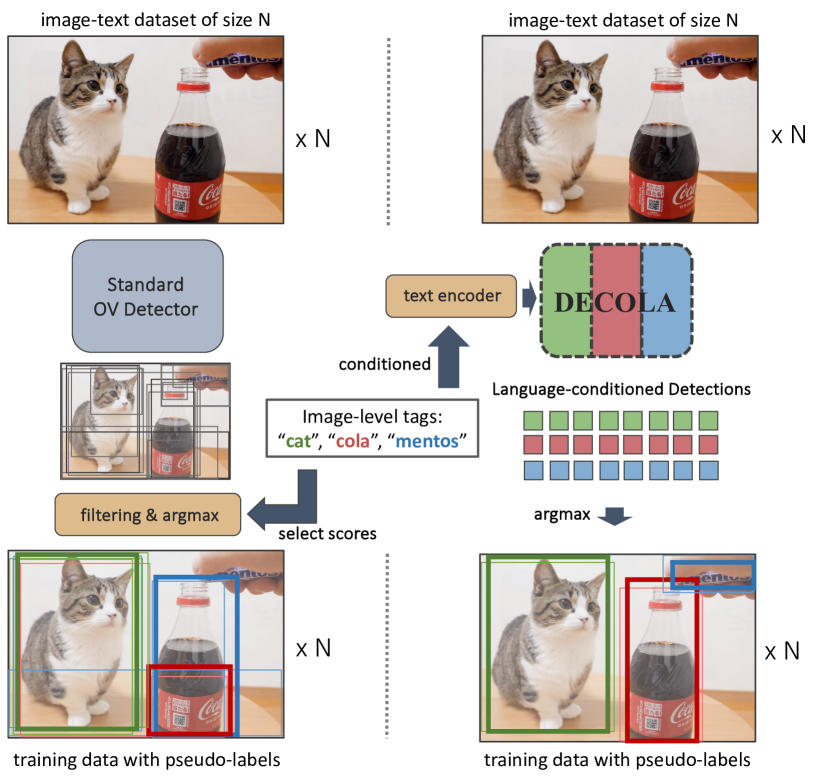
(a) Standard self-training

(b) decola self-training

Figure 1: An illustration of how standard open-vocabulary detectors and decola generate pseudo-labels using image-level data. Standard detectors use image-level information later in the pipeline after initial box proposals, which may result in low coverage of unseen classes (e.g., “mentos” and “cola”). decola adjusts the prediction to the information and ensures sufficient coverage.

Object detection has seen immense progress over the past decade. Classical object detectors reason over datasets of fixed predefined classes. This simplifies the design, training, and evaluation of new methods, and allows for rapid prototyping [18, 17, 2, 4, 73, 3, 76, 71, 43, 37, 25, 61, 5]. However, it complicates deployment to downstream applications too. A classical detector requires a new dataset to further finetune for every new concept it encounters. Collecting sufficient data for every new concept is not scalable [20]. Open-vocabulary detection offers an alternative [19, 44, 74, 67, 62, 66]. Open-vocabulary detectors reason about any arbitrary concept with free-form text, using the generalization ability of vision-language models. Yet, common open-vocabulary detectors reuse classical detectors and either replace the last classification layer with [74, 67, 19, 44], or fuse box feature with [66, 31] text representation from pretrained vision-language model. The inner workings of the detector remain unchanged.

In this paper, we introduce a transformer-based object detector that adjusts its inner workings to any arbitrary set of concepts represented in language. The detector considers only the queried set of concepts as foreground and disregards any other objects as background. It learns to adapt detection to the language embedding of queried concepts at run-time. Specifically, the detector conditions proposal generation with respect to the text embedding of each queried concept and refines the conditioned proposals into predictions. Our detection transformer conditioned on language (decola) offers a powerful alternative to classical architectures in open-vocabulary detection. Adapting the detector to language leads to stronger generalization to unseen concepts, and largely enhances self-training on weakly-labeled data.

decola’s ability to readily adapt to any queried concepts makes it particularly suitable for pseudo-labeling weakly-labeled data. Internet data, specifically images with paired text, is highly abundant and semantically rich [52, 54, 51]. The best vision models today build on this massive amount of weakly labeled data [47, 24, 34, 33, 13, 68, 10]. decola leverages the same data to produce high-quality object detection labels from image-level annotations alone. decola takes the image-level tags or text descriptions from the weakly labeled data and generates conditioned predictions as pseudo-labels. It efficiently processes multiple texts in parallel and only adds minimal computational overhead compared to the standard pseudo-labeling process. We finetune decola on this rich detection dataset of pseudo-annotations and achieve the state-of-the-art open-vocabulary detector.

We evaluate our detector on popular open-vocabulary detection benchmarks on the LVIS dataset [20, 19, 67]. The final model improves the state-of-the-art methods by 4.4 and 4.9 AP${}_{\text{novel}}$ on open-vocabulary LVIS [19] benchmark, and 5.9 and 5.4 AP${}_{\text{rare}}$ on standard LVIS [20] benchmark, with ResNet-50 [21] and Swin-B [39] backbones, respectively. Our largest model with Swin-L achieves 10.4 AP${}_{\text{rare}}$ and 3.6 mAP improvement. Furthermore, decola largely outperforms the state-of-the-art for direct zero-shot transfer benchmark on LVIS, by 12.0 and 17.1 AP${}_{\text{rare}}$ on LVIS minival and LVIS v1.0, respectively. decola consistently improves frequent, common, and rare classes altogether for different backbones and detection frameworks. Much of this improvement is driven by stronger pseudo-labeling capabilities. All our models are trained using open-sourced datasets with academic-scale computing. We open-source our code, pseudo-annotations, and checkpoints of all the model scales.

2 Related Work

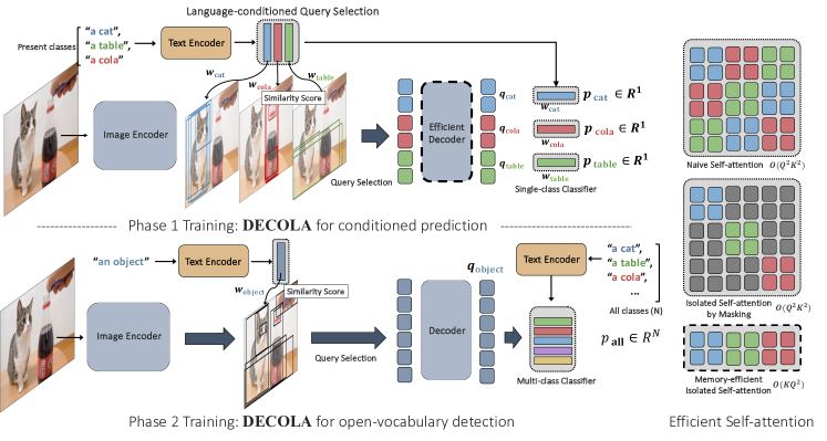
Figure 2: Overview of decola Phase 1 for conditioned prediction (top) and Phase 2 for open-vocabulary detection (bottom). For language-conditioned detection, each text embedding directly parameterizes the objectness function for each class. In Phase 2, the language-condition reads “an object” instead of particular class names, and predicts multi-class scores over all classes after decoding layers.

Open-vocabulary detection aims to detect objects of categories beyond the vocabulary of the training classes. A common solution is to inject language embeddings of class names in the last classification layer. OVR-CNN [67] pretrains a detector on image-caption data using BERT model [11] as language embedding. ViLD [19] trains a detector with CLIP text encoder [47] as language embedding with additional knowledge distillation [23] between predicted box features and the image encoder of CLIP. Detic [74] improves the above approaches through weakly-supervised learning on image-level annotations. RegionCLIP [72] introduces an intermediate pretraining step to better align CLIP to box features. BARON [62] improves the alignment between text and image encoders by extracting bag of regions as additional supervision. F-VLM [31] simplifies the training pipeline of open-vocabulary detection and explores the limit of the frozen vision-language model. All of the models above take the design of the object detector as granted, and inject language in the last classification layer of the network. We take a different approach and design a detector that adapts predictions to particular categories of interest.

Open-vocabulary DETR integrates DETR architecture into open-vocabulary detection. OWL [44] introduces a simple ViT architecture using pretrained CLIP and finetune with the DETR objective. OWLv2 uses self-training to further improve the performance [42]. OV-DETR [66] fuses features of a pretrained CLIP model with DETR object queries. Architecturally, OV-DETR is closest to decola. Both OV-DETR and decola condition predictions on the text representation of classes. OV-DETR uses the original DETR queries and expands each with a CLIP feature per class for all classes. This leads to a quadratic number of queries, growing with the original DETR queries and with the classes considered. On the other hand, decola explicitly controls the first-stage predictions (proposals) by formulating the scoring function to respect to the text embedding of each queried class at run-time. We visualize this difference in Figure 7 in the supplementary. The advantage is that we entirely remove inter-class competition and process a manageable amount of queries each focusing on a specific class, and running as fast as the vanilla Deformable DETR. This ability to freely adjust inner workings deviates decola from prior works; it expands detection data through high-quality pseudo-labeling and achieves state-of-the-art results.

Large-vocabulary object detection shares similar goals with open-vocabulary detection. Both learn from naturally long-tail data over large vocabularies. Vanilla large-vocabulary detectors are often ill-calibrated: The detector’s final classification layer favors frequently seen objects over rare ones. This imbalance is usually addressed through a change in loss [58, 56, 57, 7, 73], or leveraging additional weakly labeled data for self-training [16, 69, 77, 8]. In large-vocabulary detection, R-CNN-based frameworks [18, 17, 2, 4, 73] dominate despite DETR-style architectures [45, 71, 25, 5] having long surpassed them on standard benchmarks [36]. DETR automatically assigns object queries to output classes, and thus it learns to more heavily focus queries on common classes. We show that language-conditioning helps address this calibration issue. Specifically, it removes inter-class competition in the training objective as queries are no longer shared across categories. As a result, decola equally focuses on as many rare classes as frequent ones whenever they are present in an image. This yields a DETR-style detector that is competitive with the best R-CNN-based large-vocabulary detectors.

3 Preliminaries

Detection transformers (DETR) [3] build an object detection pipeline as a single feed-forward network. The network transforms object queries, arbitrary feature vectors, into labeled bounding boxes through a series of cross-attention layers in a decoder architecture. Vanilla DETR [3] learns object queries as free-form parameters, while modern DETRs architectures [76, 71, 25, 37, 61] adopt a two-stage paradigm similar to RCNNs [49]. This query mechanism controls much of the inner workings of the detector. Queries determine what image regions the detector focuses on, and what object classes are prioritized.

Query selection. Modern DETR architectures use image-dependent query selection, analogous to R-CNN’s proposal generation [49]. An objectness function $s$ scores each grid location $(i,j)$ in the image using a feature $x_{i,j}$ extracted from the transformer encoder. The top-$k$ scored regions proceed to the second stage as object queries $Q$:

$$s(x_{i,j})=\langle x_{i,j},w\rangle,\quad Q=\texttt{topk}_{x_{i,j}}(s(x_{i,j})).$$ (1)

Here, $w$ are the parameters of the objectness predictor. Each selected query produces a series of predictions that are refined over multiple iterations, similar to Cascade R-CNN [2]. The final prediction $\vec{p}$ contains scores over all classes $C$ and an associated box. At a high level, DETR and R-CNNs share the same motivation: first, localize all objects in a scene, then refine their predictions.

Training objective. During training, DETR assigns each object query to an object or marks it as background. This allows DETR to learn non-overlapping object queries without post-processing such as non-maximum-suppression. The Hungarian matching algorithm finds the optimal assignment between all predictions $P$ and all ground truth $G$, minimizing the loss function as matching cost:

$$\sigma^{*}=\arg\min_{\sigma\in\mathfrak{S}}\ell(P,G|\sigma)$$ (2)

where $\mathfrak{S}$ captures all possible assignments from $P$ to $G$. For each assigned prediction, the loss $\ell$ maximizes its class log-likelihood and fits its bounding box. For unassigned predictions, the loss $\ell$ reduces both the objectness score $s$ and class log-likelihood for all classes.

4 DECOLA

Our detection transformer conditioned on language, decola, changes the DETR architecture in one remarkable way: Object queries are conditioned on a language embedding. Figure 2 illustrates this change. This simple change has a few important implications: First, it allows the language embedding to control and focus queries to localize on the concepts at hand. Second, it removes any contention between different object classes. Each class present in the image uses the same amount of queries. Third, it generalizes to unseen classes by leveraging semantic knowledge encoded in language embedding throughout the detection pipeline. In the remainder of this section, we highlight the changes in the architecture and training objective for conditioning (decola Phase 1), and self-training on image-level data for open-vocabulary detection (decola Phase 2).

Language-conditioned query selection. decola conditions queries to a specific object category by modeling the objectness function as a similarity score between a region feature $x_{i,j}$ and a text representation of a category name $t(y)$ using their cosine similarity:

$$s_{y}(x_{i,j})=\frac{\langle x_{i,j},t(y)\rangle}{\|x_{i,j}\|\|t(y)\|},\;\;Q_{y}=\texttt{topk}_{x_{i,j}}(s_{y}(x_{i,j}))$$ (3)

The above objective avoids any inter-class calibration issue common in imbalanced data [58, 7, 56]. Queries do not compete, as decola independently selects top-$k$ scoring regions $Q_{y}$ for each class $y$. All queries proceed to the second stage in parallel. A memory-efficient attention mechanism isolates interaction within each class. After a series of decoding layers, each language-conditioned query predicts a single scalar score, corresponding to the likelihood of the class $y$, and the associated box. The overall architecture mirrors the two-stage deformable DETR [76] with two modifications: a language-conditioned query, and a binary output classifier.

Memory-efficient modeling. decola uses $n=|Q_{y}|$ queries per class for $K$ classes. Generally, $n$ is smaller than the total number of queries $|Q|$ of a standard DETR model. However, since we produce $n$ queries per class, the total number of queries in decola is much larger $|Q|\ll nK$. A naive implementation of the DETR decoder is unable to cope with the $O(n^{2}K^{2})$ memory requirements of the self-attention layers in the transformer decoder. We thus modify the self-attention formulation to isolate it within each class, reducing the memory cost to $O(n^{2}K)$. The actual implementation uses standard self-attention with a reshaping operation. See Figure 2 (right) for the illustration.

decola Phase 1: Train to condition on given concepts. Our goal is to design decola to take a set of class names in an image (or a batch of images) and predict objects of the corresponding classes or backgrounds. For each class $y$, each conditioned query $q_{y}\in Q_{y}$ therefore only predicts a single presence score for class $y$ and the box location. All predictions from the conditioned queries $P_{y}$ are matched with $G_{y}$, the subset of ground truth with class $y$:

$$\sigma^{*}_{y}=\arg\min_{\sigma\in\mathfrak{S}_{y}}\ell(P_{y},G_{y}|\sigma)$$ (4)

where $\mathfrak{S}_{y}$ is the set of possible matches between $P_{y}$ and $G_{y}$, and $\ell$ is the binary cross-entropy loss. Unlike the original DETR objective in Eqn. 2, Eqn. 4 matches within the conditioned class. It avoids inter-class competition during training and simplifies the training objective. Instead, it learns to adapt its predictions to $y$; the set of conditioned query $q_{y}$ considers any objects other than $y$ as background.

Pseudo-labeling weakly-labeled data. decola produces highly accurate predictions when conditioned on the exact categories of a scene, as shown in Section 5.4. This makes decola a strong pseudo-labeler for weakly-labeled data with either image tags or captions. We expand a large amount of such data with pseudo-bounding boxes of decola Phase 1 and self-train altogether to scale up open-vocabulary object detection. Unlike other forms of weakly supervised learning such as knowledge distillation [19] and online pseudo-labeling [74, 62], we simply generate labels for all images offline and jointly train over all pseudo-labeled data using the regular detection losses without any additional complication or slowdown. For each image and class $y$, decola encodes the class’ language feature and predicts a set of detections $P_{y}$. We simply choose the most confident prediction. Figure 6(d) shows our simple offline pseudo-labeling works better than online pseudo-labeling.

decola Phase 2: Train for open-vocabulary detection. The advantage of decola comes from adaptability to specified class names on a per-image basis. However, in open-vocabulary detection, the set of test classes is neither known a priori nor available per image. Hence, we convert decola into a general-purpose detector to detect all objects. We condition decola with “an object” as the text input, and inject the class information in the second-stage classifier. Figure 2 highlights this conversion. Since decola is trained to align image features to text embedding in both the first and second stages, this change only introduces inter-class calibration for multi-class object detection. We train decola with pseudo-labeled and human-labeled data as a standard supervised detection training, using the standard matching algorithm of DETR (Section 3). We do not introduce any additional hyper-parameter specifically for the weakly supervised learning [74] or design choices [31, 72], extra loss functions such as alignment loss [62], nor a large teacher model for knowledge distillation [19, 66]. Generating pseudo-labels with decola Phase 1 runs as fast as a regular detector and training Phase 2 is as easy as standard detection training on a supervised dataset. At a high level, decola Phase 1 training objective optimizes for a strong pseudo-labeler instead of a multi-class detector, which differentiates decola from prior works. Leveraging decola Phase 1 to expand weakly-labeled data is the key contribution to scaling up the final open-vocabulary object detection.

method	data	AP${}^{\text{box}}_{\text{novel}}$	AP${}^{\text{box}}_{\text{c}}$	AP${}^{\text{box}}_{\text{f}}$	mAP${}^{\text{box}}$
ResNet-50 (1K)
OV-DETR† [66]	LVIS-base, IN-21K	18.0	24.8	31.8	26.4
baseline	LVIS-base	10.2	30.9	38.0	30.1
baseline + self-train	LVIS-base, IN-21K	19.2	31.7	37.1	31.7
decola Phase 2	LVIS-base, IN-21K	23.8 (+4.6)	34.4 (+2.7)	38.3 (+1.2)	34.1 (+2.4)
ResNet-50
baseline	LVIS-base	9.4	33.8	40.4	32.2
baseline + self-train	LVIS-base, IN-21K	23.2	36.5	41.6	36.2
decola Phase 2	LVIS-base, IN-21K	27.6 (+4.4)	38.3 (+1.8)	42.9 (+1.3)	38.3 (+2.1)
Swin-B
baseline	LVIS-base	16.2	43.8	49.1	41.1
baseline + self-train	LVIS-base, IN-21K	30.8	43.6	45.9	42.3
decola Phase 2	LVIS-base, IN-21K	35.7 (+4.9)	47.5 (+3.9)	49.7 (+3.8)	46.3 (+4.0)
Swin-L
DITO⋆ [28]	O365, LVIS-base, DataComp-1B	45.8	-	-	44.2
OWLv2‡ [42]	O365, LVIS-base, VG, WebLI	45.9	-	-	50.4
baseline	O365, LVIS-base	21.9	53.3	57.7	49.6
baseline + self-train	O365, LVIS-base, IN-21K	36.5	53.5	56.5	51.8
decola Phase 2	O365, LVIS-base, IN-21K	46.9 (+10.4)	56.0 (+2.5)	58.0 (+1.5)	55.2 (+3.6)

Table 1: Open-vocabulary LVIS using DETR architectures. $\dagger$: we further finetune the official OV-DETR model trained on LVIS-base by self-training on ImageNet-21K data similar to “baseline + self-train” and decola. $\ddagger$: uses CLIP L/14, which is comparable to Swin-L backbone. $\star$: is based on Mask R-CNN with ViT L/16. We report the improvement between “baseline + self-train” to decola in green. Last 4 rows compare decola to Swin-L or equivalent scale of models that use additional detection data (e.g., Objects365, VG [30]) and billion-scale weakly-labeled data (DataComp-1B [15], WebLI [6]) for training.

method	framework	AP${}^{\text{box}}_{\text{novel}}$	mAP${}^{\text{box}}$	AP${}^{\text{mask}}_{\text{novel}}$	mAP${}^{\text{mask}}$
ViLD [19]	Mask R-CNN	16.7	27.8	16.6	25.5
RegionCLIP [72]	Mask R-CNN	-	-	17.1	22.5
DetPro [12]	Mask R-CNN	20.8	28.4	19.8	25.9
PromptDet [14]	Mask R-CNN	21.4	25.3	-	-
F-VLM [31]	Mask R-CNN	-	-	18.6	24.2
BARON [62]	Mask R-CNN	23.2	29.5	22.6	27.6
OADP [59]	Mask R-CNN	21.9	28.7	21.7	26.6
EdaDet [55]	Mask R-CNN	-	-	23.7	27.5
VLDet [35]	CenterNet2	-	-	21.7	30.1
CORA+ [63]	CenterNet2	28.1	-	-	-
Rasheed et al. [48]	CenterNet2	-	-	25.2	32.9
Detic-base [74]	CenterNet2	17.6	33.8	16.4	30.2
Detic [74]	CenterNet2	26.7	36.3	24.6	32.4
decola labels	CenterNet2	29.5	37.7	27.0	33.7

(a)

method	backbone	AP${}^{\text{box}}_{\text{novel}}$	mAP${}^{\text{box}}$	AP${}^{\text{mask}}_{\text{novel}}$	mAP${}^{\text{mask}}$
RegionCLIP [72]	R50$\times$4	-	-	22.0	32.3
CondHead [60]	R50$\times$4	24.1	33.7	24.4	32.0
ViLD [19]	EN-B7	-	-	26.3	29.3
OWL-ViT [44]	ViT-L/14	25.6	34.7	-	-
F-VLM [31]	R50$\times$64	-	-	32.8	34.9
VLDet [35]	Swin-B	-	-	26.3	38.1
3Ways [1]	NFNet-F6	30.1	44.6	-	-
RO-VIT [29]	ViT-L/16	32.1	34.0	-	-
CFM-ViT [27]	ViT-L/16	35.6	38.5	33.9	36.6
DITO [28]	ViT-B/16	34.9	36.9	32.5	34.0
CoDet [41]	Swin-B	-	-	29.4	39.2
Detic-base [74]	Swin-B	24.6	43.0	21.9	38.4
Detic [74]	Swin-B	36.6	45.7	33.8	40.7
decola labels	Swin-B	38.4	46.7	35.3	42.0

(b)

Table 2: Open-vocabulary LVIS using Mask R-CNN and CenterNet2 detectors. Methods in both tables use LVIS-base as the only human-labeled data for fair comparison. For system-level comparison (right), we include methods with non R-CNN architectures such as OWL-ViT [44]. The results show the impact of high-quality pseudo-labels generated by decola Phase 1.

method	data	AP${}^{\text{box}}_{\text{rare}}$	mAP${}^{\text{box}}$
ResNet-50
baseline	LVIS	26.3	35.6
baseline + self-train	LVIS, IN-21K	30.0	36.6
decola Phase 2	LVIS, IN-21K	35.9 (+5.9)	39.4 (+2.8)
Swin-B
baseline	LVIS	38.3	44.5
baseline + self-train	LVIS, IN-21K	42.0	45.2
decola Phase 2	LVIS, IN-21K	47.4 (+5.4)	48.3 (+3.1)
Swin-L
baseline	O365, LVIS	49.3	54.4
baseline + self-train	O365, LVIS, IN-21K	48.7	53.4
decola Phase 2	O365, LVIS, IN-21K	54.9 (+6.2)	56.4 (+3.0)

(a)

method	AP${}^{\text{box}}_{\text{rare}}$	mAP${}^{\text{box}}$	AP${}^{\text{mask}}_{\text{rare}}$	mAP${}^{\text{mask}}$
ResNet-50
Detic-base [74]	28.2	35.3	25.6	31.4
Detic [74]	31.4	36.8	29.7	33.2
decola labels	35.6 (+4.2)	38.6 (+1.8)	32.1 (+2.4)	34.4 (+1.2)
Swin-B
Detic-base [74]	39.9	45.4	35.9	40.7
Detic [74]	45.8	46.9	41.7	41.7
decola labels	47.6 (+1.8)	48.5 (+1.6)	43.7 (+2.0)	43.6 (+1.9)

(b)

Table 3: Standard LVIS benchmark. decola shows consistent improvement over different model scales and architectures.

5 Experiments

We evaluate the effectiveness of decola in two aspects: (1) pseudo-labeling quality of decola Phase 1 (Section 5.4) and (2) benchmark evaluation (Section 5.3). We consider three primary benchmarks to evaluate our final model (decola Phase 2): open-vocabulary LVIS [19], standard LVIS [20], and direct zero-shot evaluation to LVIS, COCO [36], Object365 [53], and OpenImages [32].

5.1 Experimental Setup

Datasets and benchmarks. We mainly evaluate our method on the LVIS dataset [20], a large-vocabulary instance segmentation and object detection dataset with 1203 naturally distributed object categories. LVIS splits categories into frequent, common, and rare. For open-vocabulary LVIS, we combine frequent and common categories into LVIS-base and consider the rare categories as novel concepts used for testing only [19]. For standard LVIS, we train and evaluate all classes. Direct zero-shot transfer evaluates models trained on different detection data (e.g., Object365) and other weakly-labeled data without any prior knowledge about the target dataset such as the set of classes or object frequency. In this benchmark, we test decola’s generalization to different domains. We evaluate decola on LVIS, COCO [36], Object365 [53], and OpenImages [32] in a fully zero-shot manner. All our models use the ImageNet-21K [51] dataset as weakly labeled data, which contains 14M of object-centric images annotated with a single class.

Evaluation metrics. We evaluate decola on AP${}_{\text{novel/rare}}$, AP${}_{\text{c}}$, AP${}_{\text{f}}$, and mAP following the LVIS evaluation metric [20]. We highlight the results in all three groups since we believe open-vocabulary detectors should not compensate for the performance of common/frequent classes for novel/rare classes. We evaluate both AP${}^{\text{box}}$ and AP${}^{\text{mask}}$ for object detection and instance segmentation. For zero-shot transfer benchmark with COCO and Object365, we use AP, AP₅₀, and AP₇₅ following prior work [19, 74]. For OpenImages, we report AP${}_{50}^{\text{flat}}$ on the expanded label space [74, 75]. For zero-shot transfer to LVIS, we consider LVIS minival [26] and standard LVIS v1.0 validation set and report AP${}^{\text{fixed}}$ [9] following the prior works [26, 34, 38]. In addition, we pursue a more direct measurement of the generated pseudo-labeling quality. Hence, we define conditioned mAP/AR (c-mAP/AR) and compare it to baseline open-vocabulary detectors. c-mAP measures the detection performance in mAP when the detector is provided the set of ground truth classes in each image. For example in Figure 1, both detectors use “cat”, “mentos” and “cola” as given. This extra information is used to select scores to rank the final predictions (baselines), or directly condition the detector (decola). We analyze the model’s behavior and label quality in Section 5.4 and Section 9 in supplementary.

		LVIS minival				LVIS v1.0 val
method	data	AP${}^{\text{box}}_{\text{rare}}$	AP${}^{\text{box}}_{\text{c}}$	AP${}^{\text{box}}_{\text{f}}$	mAP${}^{\text{box}}$	AP${}^{\text{box}}_{\text{rare}}$	AP${}^{\text{box}}_{\text{c}}$	AP${}^{\text{box}}_{\text{f}}$	mAP${}^{\text{box}}$
Swin-T
MDETR⋆ [26]	LVIS, GoldG, RefC	20.9	24.9	24.3	24.2	7.4	22.7	25.0	22.5
GLIP [34]	O365, GoldG, Cap4M	20.8	21.4	31.0	26.0	10.1	12.5	25.5	17.2
GroundingDINO [38]	O365, GoldG, Cap4M	18.1	23.3	32.7	27.4	-	-	-	-
GLIPv2 [70]	O365, GoldG, Cap4M	-	-	-	29.0	-	-	-	-
MQ-GroundingDINO† [65]	O365, GoldG, Cap4M, LVIS-5VQ	21.7	26.2	35.2	30.2	12.9	17.4	31.4	22.1
MQ-GLIP† [65]	O365, GoldG, Cap4M, LVIS-5VQ	21.0	27.5	34.6	30.4	15.4	18.4	30.4	22.6
decola Phase 2	O365, IN-21K‡	32.8	32.0	31.8	32.0	27.2	24.9	28.0	26.6
$\Delta$		(+12.0)	(+8.7)	-	(+3.0)	(+17.1)	(+12.4)	(+2.5)	(+9.4)
Swin-L
GLIP [34]	FourODs, GoldG, Cap24M	28.2	34.3	41.5	37.3	17.1	23.3	35.4	26.9
GroundingDINO [38]	O365, OI, GoldG, Cap4M, COCO, RefC	22.2	30.7	38.8	33.9	-	-	-	-
MQ-GLIP† [65]	FourODs, GoldG, Cap24M, LVIS-5VQ	34.5	41.2	46.9	43.4	26.9	32.0	41.3	34.7
OWLv2 [42]	O365, VG, WebLI	39.0	-	-	38.1	34.9	-	-	33.5
decola Phase 2	O365, OI, IN-21K‡	41.5	38.0	34.9	36.8	32.9	29.1	30.3	30.2
$\Delta$		(+2.5)	(+3.7)	-	-	-	(+5.8)	-	-

Table 4: Direct zero-shot transfer to LVIS. $\dagger$: methods use 5 per-class vision queries of LVIS dataset (denoted as “LVIS-5VQ”), which use images and annotations to extract instance-level features. $\star$: MDETR uses ResNet-101 backbone and trained fully-supervised on LVIS. Results that use LVIS data are in gray. $\ddagger$: Full ImageNet-21K. No LVIS information is used in decola.

	COCO			O365			OI
method	AP	AP50	AP75	AP	AP50	AP75	AP${}^{\text{flat}}_{50}$
R-CNNs
ViLD [19]	36.6	55.6	39.8	11.8	18.2	12.6	-
F-VLM [31]	32.5	53.1	34.6	11.9	19.2	12.6	-
DetPro [12]	34.9	53.8	37.4	12.1	18.8	12.9	-
BARON [62]	36.3	56.1	39.3	13.6	21.0	14.5	-
Detic [74]	39.1	56.3	42.2	14.2	20.7	15.2	42.9
DETRs
OV-DETR [66]	38.1	58.4	41.1	-	-	-	-
Detic [74]	39.8	56.6	43.3	14.5	21.4	15.5	41.6
decola Phase 2	40.3	57.0	43.7	15.0	22.0	16.0	43.3

Table 5: Cross-dataset generalization benchmark on COCO, Object365, and OpenImages. All models use a ResNet-50 backbone and train on LVIS-base and weakly-labeled data.

5.2 Models

decola is based on two-stage Deformable DETR [76]. As described in Section 4, the first-stage objectness function for query selection is replaced by a similarity score between the image feature and the CLIP text embedding of each class name. We train the detector with the improved DETR training recipe [71, 45]: look-forward-twice, larger MLP hidden dimension, no dropout, etc. We consider four backbones: a ResNet-50 [21], Swin-B and L for all LVIS benchmarks, and Swin-T and L for the direct zero-shot transfer. Unless otherwise mentioned, all backbones are pretrained on the ImageNet-21K dataset [50]. Next, we describe our key baseline models to directly compare to decola.

Baseline. We design a baseline open-vocabulary detector to closely compare to decola. Inspired by Detic [74], baseline replaces classification layers with the class embedding of the pretrained CLIP text encoder and is trained using Federated Loss [73]. decola Phase 1 and baseline are trained using human-labeled data (e.g., LVIS-base). All other settings (training dataset, number of training iterations, etc.) are kept the same between decola and baseline.

Baseline + self-train. Similar to decola Phase 2, we self-train baseline on weakly-labeled data. For the self-training algorithm, we use online self-training with max-size loss from Detic [74] as baseline comparison (baseline + self-train) to decola Phase 2. We tested max-size and max-score losses from Detic [74] (online pseudo-labeling) as well as offline pseudo-labeling similar to decola, and max-size loss consistently performed the best.

decola labels. We train a two-stage detector for broader comparison: CenterNet2 [73]. Specifically, we use Detic’s baseline model (“Detic-base”), a CenterNet2 trained on LVIS-base with CLIP embedding, and finetune on pseudo-labeled ImageNet-21K data using decola Phase 1 of the same backbone size. We denote this as “decola labels”.

Efficient modeling. For decola Phase 1, we use $n=300$ queries per class. One memory and time bottleneck during decola training is the first-stage loss computation. The original Deformable DETR computes Hungarian matching with all pixels to all objects in a class-agnostic manner, which is $\sum_{l\in L}H_{l}\cdot W_{l}$ predictions. To reduce the memory and time cost, we only consider the top $K=10,000$ confident pixels for each class $y$ during the first-stage matching and loss computation. Together with memory-efficient self-attention (Sec. 4), the training time and memory cost of decola increases by less than $20\%$ over the baselines (See Table 6).

Training details. Following Detic [74], we train decola Phase 1 and baseline $4\times$ on LVIS-base, and further finetune for another $4\times$ on ImageNet-21K data with pseudo-labeling. For training CenterNet2 with decola labels, we combine pseudo-labels from different image resolutions for $h\in\{240,280,320,360,400\}$, where $h$ is the shorter side of the image. Note that this mimics the random image resizing data augmentation during standard detection training. We use Detectron2 [64] based on PyTorch [46] in all of the experiments. More details are in Section 8 of supplementary.

5.3 Main Results

Open-vocabulary LVIS. Table 1 compares decola to baseline as well as state-of-the-art DETR-based open-vocabulary detectors; OV-DETR [66], OWLv2 [42], and baseline + self-train. For a fair comparison, we further finetune the official OV-DETR model checkpoint on ImageNet-21K for 4$\times$ schedule same as decola Phase 2 and baseline + self-train. For all backbone scales, we show consistent improvement over other methods. Notably, baseline + self-train exhibits degradation in frequent classes as a trade-off with improved novel classes, which is commonly observed behavior in other open-vocabulary detection methods, too. decola improves all categories consistently, which highlights the quality of our pseudo-labels. In the last rows with the Swin-L backbone, we report the result of two concurrent works, DITO [28] (Mask R-CNN-based) and OWLv2, to compare to the method that uses additional detection data (Object365) and billion-scale web data (DataComp-1B [15], WebLI [6]). decola demonstrates large improvement over the state-of-the-arts despite using orders of magnitude smaller training data and compute resources. To further examine decola’s scalability, we test the pseudo-labeling capability of decola on R-CNN-based detectors with decola labels (Detic-base finetuned with our pseudo-labels). In Table 2, we compare decola labels to a broad range of literature based on CenterNet2 [73] and Mask R-CNN [22]. Table LABEL:tab:c2_r50 compares methods with ResNet-50 backbone and Table LABEL:tab:c2_sys compares larger scale backbones for system-level comparison. In both tables, decola clearly improve upon the state-of-the-art by large margins without additional complication in training and bells-and-whistles.

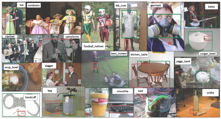
Figure 5: Examples of prediction on unseen categories. Images from ImageNet-21K dataset. Boxes are the most confident prediction from decola and baseline. decola conditions on the ground truth label, and baseline selects the max-score box of the ground truth class. Images are all from unseen categories, which neither model was trained on. Green: decola Phase 1 trained on LVIS-base. Red: baseline trained on LVIS-base. Both models use a Deformable DETR detector with a ResNet-50 backbone. More in Fig. 14 and  15 of supplementary.

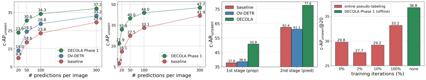
(a) c-AP for ResNet-50 (IN-1K)

(b) c-AP for Swin-B

(c) c-AR for 1st and 2nd stage boxes

(d) online vs offline: c-AP$@20$

Figure 6: Analyzing decola. All plots show the conditioned AP/AR for unseen classes. We compare decola Phase 1 and baselines. We highlight more detailed analyses about c-AP and c-AR in Section 9, Table 8 and 9 of the supplementary materials.

	train		test
method	time	mem.	time	mem.
baseline	44 h	8.9 G	0.07 s/img	2.5 G
+ self-train	45 h	10.2 G	0.07 s/img	2.5 G
OV-DETR	73 h	22.0 G	6.4 s/img	3.4 G
decola Phase 1	49 h	12.6 G	-	-
decola Phase 2	45 h	8.9 G	0.07 s/img	2.8 G

Table 6: Efficiency. Training time is measured with 8 DGX V100 on ResNet-50, 2 images per-GPU. float16 is used in both training and testing. OV-DETR uses the original optimized inference.

Standard LVIS. Tables 3 evaluate decola and baseline on the standard LVIS benchmark, where all object categories are used to fully supervise the detectors. Similar to the open-vocabulary LVIS, we compare DETR architectures in Table LABEL:tab:st_detr and R-CNN architectures in Table LABEL:tab:st_c2. Table LABEL:tab:st_detr shows that decola remarkably improves baseline by 9.5, 9.1, and 5.6 points on AP${}^{\text{box}}_{\text{rare}}$, outperforming baseline + self-train by 5.9, 5.4, and 6.2 AP${}^{\text{box}}_{\text{rare}}$ for ResNet-50, Swin-B, and Swin-L backbones, respectively. Similarly in Table LABEL:tab:st_c2, decola labels further improves the baseline of Detic by 7.4 and 7.7 AP${}^{\text{box}}_{\text{rare}}$, and outperforms Detic [74] by 4.2 and 1.8 AP${}^{\text{box}}_{\text{rare}}$ with ResNet-50 and Swin-B backbones, respectively.

Direct zero-shot evaluation. For direct zero-shot evaluation, we train decola with Swin-T [39] and use Object365 data for Phase 1, and ImageNet-21K for Phase 2 (full dataset and classes). We compare to MDETR [26], GLIP [34], GroundingDINO [38], and MQ-Det [65] finetuned from GLIP and GroundingDINO. Table 4 shows the results. decola outperforms the previous state-of-the-arts, by 12.0/17.1 AP${}_{\text{rare}}$ and 3.0/9.4 mAP on LVIS minival and LVIS v1.0 val, respectively. It is noteworthy that all other methods use much richer detection labels from GoldG data [26], a collection of grounding data (box and text expression pairs) curated by MDETR. Furthermore, other benchmark methods show highly imbalanced AP${}_{\text{rare}}$ and AP${}_{\text{f}}$ in both LVIS minival and LVIS v1.0 val (10-20 points gap). We hypothesize that the large collection of training data coincides with LVIS vocabulary, as all data follows a natural distribution of common objects. Also, decola enjoys significantly faster run-time compared to all other models that undergo BERT encoding for grounding, which requires more than 50 forward passes per image in order to predict all LVIS categories. Similarly, our Swin-L model outperforms GroundingDINO and GLIP by 19.3 and 13.3 AP${}_{\text{rare}}$, respectively, despite much smaller training data compared to FourODs [34] and match to OWLv2 with 10-B private WebLI data [6]. Table 5 further examines the generality of decola on different domains. decola Phase 2 with ResNet-50 outperforms all other competitive baselines by a large margin for both R-CNN and DETR architectures.

5.4 Analyses

In this section, we analyze the model’s behavior with conditioned mAP/AR (c-AP/AR) (defined in Sec. 5.1).

Pseudo-labeling quality. Figure 6(a) and 6(b) compare decola Phase 1, OV-DETR, and baseline on c-AP for unseen classes. Compared to baseline and OV-DETR, decola Phase 1 generates much higher quality pseudo-labels, especially in low-shot regimes. See examples in Figure 5.

Impact of conditioning. In Figure 6(c), we compare c-AR of unseen classes. This measures the detector’s ability to localize objects of interest when pseudo-labeling. We observe significant improvement in c-AR on both first-stage (proposals) and second-stage (predictions) due to our conditioning mechanism. This result demonstrates the key difference between decola and other open-vocabulary detectors.

Pseudo-labeling algorithms. Figure 6(d) shows the c-AP of baseline + self-train and decola Phase 1 for unseen classes with 20 predictions per-image. Each red bar indicates the percent of training iteration during self-training. Online self-labeling suffers a sharp drop during the early iterations, and c-AP after full iterations still underperforms compared to decola Phase 1. decola’s simple approach of offline self-training is more stable and effective.

6 Conclusion

In this paper, we explore a new open-vocabulary detection framework, decola. It adjusts its inner workings to the concepts that the user asks to reason over by conditioning on a language embedding. Our detector generates high-quality pseudo-labels on weakly labeled data through the conditioning mechanism. We finetune it with the pseudo-labels to build the state-of-the-art open-vocabulary detector.

Acknowledgement. We thank Xingyi Zhou for his valuable feedback, and Yue Zhao, Jeffrey Ouyang-Zhang, and Nayeon Lee for fruitful discussions. This material is in part based upon work supported by the National Science Foundation under Grant No. IIS-1845485 and IIS-2006820.

Supplementary Material

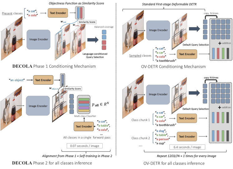
Figure 7: Difference in conditioning mechanism and multi-class inference between decola and OV-DETR. decola produces different proposals for each present object class in image by modeling the objectness function with the similarity score between text embedding and proposal feature. OV-DETR copies object queries from the first-stage DETR and add CLIP features. Bottom row illustrates how decola and OV-DETR performs multi-class detection.

7 Comparing to OV-DETR [66].

Conditioning mechanism. Figure 7 illustrates the difference in conditioning mechanism and multi-class inference between decola and OV-DETR. During training Phase 1, decola learns to use text embedding of each present object class in order to locate proposals. decola learns dense language-vision alignment by modeling the objecness function as the similarity score between text embedding and proposal features defined as equation 3 in the Section 4 of the main paper. decola transforms equal number of proposals into query embedding to sufficiently cover all classes. On the other hand, OV-DETR trains with the same DETR object queries and add CLIP features of randomly sampled object classes. This difference results in a significant improvement in conditioned AP and AR (+9.1 c-AP_@20, +16.5 c-AR), as shown in Figure 6(a) and 6(c) of the main paper.

Multi-class detection. decola finetunes for multi-class object detection during Phase 2 whereas OV-DETR maintains the original conditioning mechanism for finetuning. Finetuning with multi-class detection objective is critical for the final detection task: Detector needs to calibrate the multi-class scores over the dataset-level vocabulary to maximize mAP. OV-DETR trains with randomly sampled set of classes every iteration, which makes it unable to properly rank objects over all classes. This leads to a severe degradation in frequent classes as shown in Table 1 of the main paper. Moreover, the conditioning mechanism of OV-DETR requires splitting the text vocabulary over multiple chunks. For LVIS dataset, OV-DETR needs about 40 forward passes for every image at inference, leading to a substantial difference in speed at run-time (0.07 vs 6.4 sec / img) as shown in Table 6 of the main paper. The final models, decola Phase 2 and OV-DETR^† under identical training and architectural settings, exhibit large difference of 5.8 AP${}_{\text{novel}}$ and 7.7 mAP, as shown in Table 1 of the main paper.

Training setup. Both models are trained on LVIS-base for $4\times$ (decola Phase 1 and OV-DETR). OV-DETR undergoes extra $4\times$ with the original self-training using CLIP labeling [66]. This model is the same as the original OV-DETR reported in the original paper. We further finetune decola and OV-DETR on ImageNet-21K for $4\times$ for fair comparison, which result decola Phase 2 and OV-DETR^†.

8 Experimental Details

Training configuration. We closely follow [74] to train decola as well as baseline for both Deformable DETR and CenterNet2 results. Table LABEL:tab:training_configs and LABEL:tab:model_configs highlight important hyper-parameters in all experiments with Deformable DETR. For experiments with CenterNet2, we follow the same training and model configuration as Detic [74]. For all experiments, we used 8 V100 GPUs with 32G memory. All models are trained on float16 using Automatic Mixed Precision from PyTorch [46]. With this computing environment, training decola for Deformable DETR with ResNet-50 backbone takes about 50 hours and the baseline takes about 45 hours for $4\times$ training schedule. For ImageNet-21K pre-trained ResNet-50, we used the model from Ridnik et al. [50] consistent with [74]. Our codebase uses Detectron2 [64] based on PyTorch [46]. For direct zero-shot transfer to LVIS experiments, we use Swin-T and L [39] pretrained on ImageNet-21K. For both methods, we train Phase 1 on Object365 same number of iterations as GLIP [34]. We finetune Phase 2 on the entire ImageNet-21K for Swin-T, and ImageNet-21K and OpenImages [32] for the same number of iterations as Phase 1. Please note that the model may continue to improve as training longer. Swin-L model is trained with 2 nodes of 8 V100 machines, with 32 images per global batch. All our experiments are conducted under academic-scale compute and open-sourced datasets.

config	baseline training	baseline + self-train
shared configuration
optimizer	AdamW [40]	AdamW [40]
optimizer momentum	$\beta_{1},\beta_{2}=0.9,0.999$	$\beta_{1},\beta_{2}=0.9,0.999$
weight decay	0.0001	0.0001
total iterations	360000	360000
base learning rate	0.0002	0.0002
learning rate schedule	step decay	step decay
learning rate decay factor	0.1	0.1
learning rate decay step	300000	300000
gradient clip value	0.01	0.01
gradient clip norm	2.0	2.0
different configuration
batch size	16	(16, 64)
dataset ratio	n/a	$1:4$ [74]
image min-size range	(480, 800)	((480, 800), (240, 400)) [74]
image max-size	1333	(1333, 667) [74]
input augmentation	DETR-style [3]	resize shortest edge [74]
input sampling	repeated factor sampling [20]	(repeated factor [20], random)

(a)

config	baseline	decola Phase 1	decola Phase 2
shared configuration
cls weight	2.0	2.0	2.0
giou weight	2.0	2.0	2.0
l1 weight	5.0	5.0	5.0
two-stage	True	True	True
box refinement	True	True	True
feed-forward dim.	1024	1024	1024
look-forward-twice	True	True	True
drop-out rate	0.0	0.0	0.0
different configuration
number of queries	300	300 per class	300
classification loss type	federated loss [73]	biniary cross-entropy	federated loss [73]
1st-stage classifier type	learnable	“a [class name].”	“an object.”
1st-stage classifier norm	n/a	L2	L2
1st-stage classifier temp.	n/a	50	50
1st-stage top-$k$ per class†	n/a	10000	n/a
2nd-stage classifier type	“a [class name].”	“a [class name].”	“a [class name].”
2nd-stage classifier norm	L2	L2	L2
2nd-stage classifier temp.	50	50	50
classifier $\#$ classes‡	1203	1	1203
classifier bias init. value	$-\log(0.99/0.01)$	$-\log(0.99/0.01)$	$-\log(0.99/0.01)$

(b)

Table 7: Configurations. Training and model details for experiments with Deformable DETR. $\dagger$ is the top-$k$ only for Hungarian matching and loss computation to reduce computation, as explained in the main paper. $\ddagger$ is for LVIS experiments. Here decola for language-condition training has $\#$ classes as 1, since the second-stage with language-conditioned query is binary classification as opposed to multi-class classification in baseline and open-vocabulary detection.

model	data	c-AP${}_{\text{novel}}^{\text{box}}$@10	c-AP${}_{\text{novel}}^{\text{box}}$@20	c-AP${}_{\text{novel}}^{\text{box}}$@50	c-AP${}_{\text{novel}}^{\text{box}}$@100	c-AP${}_{\text{novel}}^{\text{box}}$@300
ResNet-50
baseline	LVIS-base	6.0	11.3	19.2	26.8	31.9
decola Phase 1	LVIS-base	19.4 (+13.4)	28.5 (+17.2)	34.1 (+14.9)	38.7 (+11.9)	40.0 (+8.1)
Swin-B
baseline	LVIS-base	7.4	16.1	27.5	33.1	41.9
decola Phase 1	LVIS-base	21.9 (+14.5)	32.0 (+15.9)	40.0 (+12.5)	44.0 (+6.9)	47.7 (+5.8)

(a)

model	data	c-AP${}_{\text{rare}}^{\text{box}}$@10	c-AP${}_{\text{rare}}^{\text{box}}$@20	c-AP${}_{\text{rare}}^{\text{box}}$@50	c-AP${}_{\text{rare}}^{\text{box}}$@100	c-AP${}_{\text{rare}}^{\text{box}}$@300
ResNet-50
baseline	LVIS	21.3	29.4	36.9	41.1	44.6
decola Phase 1	LVIS	26.6 (+5.3)	39.1 (+9.7)	45.2 (+8.3)	47.1 (+6.0)	48.8 (+4.2)
Swin-B
baseline	LVIS	30.1	38.2	45.5	49.3	53.2
decola Phase 1	LVIS	33.5 (+3.4)	43.9 (+5.7)	51.4 (+5.9)	53.8 (+4.5)	55.8 (+2.6)

(b)

Table 8: Conditioned AP${}_{\text{rare/novel}}$ result of decola Phase 1 and baseline pre-trained on LVIS-base (top) and LVIS (bottom). Conditioned AP measures detection performance when the set of object categories present in each image is given. baseline adapts its classification layer to the classes and decola conditions itself to the classes, as described in Section 4 of the main paper.

model	data	c-mAP${}^{\text{box}}$@10	c-mAP${}^{\text{box}}$@20	c-mAP${}^{\text{box}}$@50	c-mAP${}^{\text{box}}$@100	c-mAP${}^{\text{box}}$@300
ResNet-50
baseline	LVIS-base	24.4	29.8	35.0	37.9	40.2
decola Phase 1	LVIS-base	30.0 (+5.6)	36.8 (+7.0)	41.9 (+6.9)	44.2 (+6.3)	45.6 (+5.4)
Swin-B
baseline	LVIS-base	29.6	36.9	43.4	46.0	48.8
decola Phase 1	LVIS-base	33.5 (+3.9)	41.3 (+4.4)	47.4 (+4.0)	49.7 (+3.7)	51.5 (+2.7)

(a)

model	data	c-mAP${}^{\text{box}}$@10	c-mAP${}^{\text{box}}$@20	c-mAP${}^{\text{box}}$@50	c-mAP${}^{\text{box}}$@100	c-mAP${}^{\text{box}}$@300
ResNet-50
baseline	LVIS	27.3	33.4	38.8	41.2	43.1
decola Phase 1	LVIS	31.1 (+3.8)	38.5 (+5.1)	43.7 (+4.9)	45.6 (+4.4)	47.1 (+4.0)
Swin-B
baseline	LVIS	33.3	40.4	46.2	48.6	50.5
decola Phase 1	LVIS	35.7 (+2.4)	43.6 (+3.2)	49.4 (+3.2)	51.6 (+3.0)	53.2 (+2.7)

(b)

Table 9: Conditioned mAP result of decola in phase 1 and baseline pre-trained on LVIS-base (top) and LVIS (bottom). Conditioned mAP measures detection performance when the set of object categories present in each image is known. baseline adapts its classification layer to the classes and decola condition itself to the classes, as described in Section 4 of the main paper.

model	reg. loss	AP${}^{\text{box}}_{\text{novel}}$	mAP${}^{\text{box}}$
decola label		27.6	36.6
decola label	✓	29.5	37.7

(a)

model	AP${}^{\text{box}}_{\text{novel}}$	mAP${}^{\text{box}}$
baseline + decola label	25.1	36.9
decola Phase 2	27.6	38.3

(b)

type	c-AP${}^{\text{box}}_{\text{novel}}$	c-mAP${}^{\text{box}}$
multi	14.2	20.7
single	28.5	40.0

(c)

type	c-AP${}_{\text{novel}}^{\text{box}}$	c-mAP${}^{\text{box}}$
base	20.9	30.4
text	21.2	31.6
image	22.3	35.1

(d)

$p$	c-AP${}_{\text{novel}}^{\text{box}}$	mAP${}^{\text{box}}$
$1.0$	10.7	30.2
$0.5$	19.1	30.2
$0.0$	22.3	n/a

(e)

$p$	AP${}_{\text{novel}}^{\text{box}}$	AP${}_{\text{c}}^{\text{box}}$	AP${}_{\text{f}}^{\text{box}}$	mAP${}^{\text{box}}$
$0.5\rightarrow 0.5$	21.0	31.9	37.0	32.0
$0.5\rightarrow 1.0$	20.8	33.2	37.8	32.9
$0.0\rightarrow 1.0$	23.8	34.4	38.3	34.1

(f)

Table 10: Additional results. open-vocabulary LVIS results for various ablation study. We used Deformable DETR with ResNet-50 for all models here. For all results with c-AP, we use Phase 1. $k$ represents the detection limit per image. Note that the bottom row tables (d), (e), (f) are trained with decola and baseline trained using ResNet-50 pretrained with ImageNet-1K.

model	data	$n=1$	$n=2$	$n=5$	$n=10$	$n=20$
ResNet-50
baseline	LVIS-base	14.7	22.4	27.6	30.9	32.2
decola Phase 1	LVIS-base	25.2 (+10.5)	31.4 (+9.0)	36.0 (+8.4)	37.9 (+7.0)	39.9 (+7.7)
Swin-B
baseline	LVIS-base	17.8	26.0	33.7	37.6	40.9
decola Phase 1	LVIS-base	31.0 (+13.2)	37.3 (+11.3)	44.1 (+10.4)	46.2 (+8.6)	47.2 (+6.3)

(a)

model	data	$n=1$	$n=2$	$n=5$	$n=10$	$n=20$
ResNet-50
baseline	LVIS	17.8	24.8	33.0	38.7	42.3
decola Phase 1	LVIS	29.7 (+11.9)	36.7 (+11.9)	41.8 (+8.8)	45.9 (+7.2)	48.3 (+6.0)
Swin-B
baseline	LVIS	20.7	29.9	42.4	48.4	51.6
decola Phase 1	LVIS	34.5 (+13.8)	42.3 (+12.4)	49.0 (+6.6)	50.8 (+2.4)	52.7 (+1.1)

(b)

Table 11: decola is more box-efficient (c-AP${}_{\text{rare/novel}}$). We measure conditioned AP of rare/unseen classes (c-AP${}_{\text{rare/novel}}$) of decola Phase 1 and baseline pre-trained on LVIS-base (top) and LVIS (bottom) with different per-class number of query. decola uses $n=|Q_{y}|$ language-conditioned queries for each class in image. Baseline uses $n\cdot|C_{x}|$ object queries where $C_{x}$ is the set of object classes in image $x$. Two models use the same total number of object queries.

model	data	$n=1$	$n=2$	$n=5$	$n=10$	$n=20$
ResNet-50
baseline	LVIS-base	14.8	22.2	29.6	33.6	35.2
decola Phase 1	LVIS-base	24.5 (+9.7)	31.5 (+9.3)	37.9 (+8.3)	41.1 (+7.5)	43.4 (+8.2)
Swin-B
baseline	LVIS-base	18.0	26.9	36.6	41.0	43.4
decola Phase 1	LVIS-base	28.0 (+10.0)	35.2 (+8.3)	42.7 (+6.1)	46.5 (+5.5)	48.9 (+5.5)

(a)

model	data	$n=1$	$n=2$	$n=5$	$n=10$	$n=20$
ResNet-50
baseline	LVIS	15.0	22.6	31.1	35.7	38.3
decola Phase 1	LVIS	25.5 (+10.5)	32.2 (+9.6)	38.9 (+7.8)	42.6 (+6.9)	44.8 (+6.5)
Swin-B
baseline	LVIS	18.3	27.2	37.6	42.4	44.4
decola Phase 1	LVIS	29.3 (+11.0)	36.8 (+9.6)	44.0 (+6.4)	47.7 (+5.3)	50.1 (+5.7)

(b)

Table 12: decola is more box-efficient (c-mAP). We measure Conditioned mAP of decola Phase 1 and baseline pre-trained on LVIS-base (top) and LVIS (bottom) with different per-class number of query. decola uses $n=|Q_{y}|$ language-conditioned queries for each class in image. Baseline uses $n\cdot|C_{x}|$ object queries where $C_{x}$ is the set of object classes in image $x$. Two models use the same total number of object queries. Conditioned mAP measures with $k=300$ per-image detection limit.

method	pretrain	AP${}^{\text{box}}_{\text{novel}}$	AP${}^{\text{box}}_{\text{c}}$	AP${}^{\text{box}}_{\text{f}}$	mAP${}^{\text{box}}$
baseline	IN-1K	10.2	30.9	38.0	30.1
	RegionCLIP [72]	9.1	32.6	39.9	31.4
	IN-21K	9.4 (-0.8)	33.8 (+2.9)	40.4 (+2.4)	32.2 (+2.1)
baseline + self-train	IN-1K	19.2	31.7	37.1	31.7
	IN-21K	23.2 (+4.0)	36.5 (+4.8)	41.6 (+4.5)	36.2 (+4.5)
decola Phase 2	IN-1K	23.8	34.4	38.3	34.1
	IN-21K	27.6 (+3.8)	38.3 (+3.9)	42.9 (+4.6)	38.3 (+4.2)

(a)

method	O365	c-AP${}_{\text{rare}}^{\text{box}}$@300	c-AP${}_{\text{c}}^{\text{box}}$@300	c-AP${}_{\text{f}}^{\text{box}}$@300	c-mAP${}^{\text{box}}$@300
decola Phase 1		54.6	52.7	52.3	52.9
	✓	62.0 (+7.4)	62.0 (+9.3)	61.6 (+9.3)	61.8 (+8.9)

(b)

Table 13: Impact of different pretraining. Evaluated on open-vocabulary LVIS with ResNet-50 Deformable DETR (top) and large-vocabulary LVIS with Swinl-L Deformable DETR (bottom). We explore the impact of different pretraining on the final mAP (top) and conditioned AP (bottom).

9 Additional Experimental Results

Conditioned AP. Table 8 and 9 compare conditioned mAP and AP${}_{\text{novel}}$ of baseline and decola Phase 1. We show AP with different per image detection limit, reported with $@k$. Conditioned AP is defined in Section 5.1. Results at low detection limit follows more closely to the labeling quality; pseudo-labels are sampled based on the confidence score and typically only save the top-1 prediction. decola consistently improve baseline not only for novel classes but for overall. This difference is the core reason for decola’s scalability by self-training.

Box-efficient detector. In this section, we highlight an interesting property of decola. Object detectors for large-vocabulary dataset often tend to over-shoot predictions with a high number of boxes in order to increase recall for rare object classes. This behavior may be undesirable since lots of spammed boxes makes it difficult to interpret for downstream tasks. Therefore, Table 11 and 12 report c-AP of baseline and decola Phase 1 with a limited number of query (prediction) per class. $n=1$ means the detector only gets to predict a single box for each class present in image. Please recall that c-AP provides a set of present classes during inference. We show that decola show highly accurate predictions with low per-image detection limit.

Impact of different pre-training. Table 13 shows how backbone pretraining impact the final result on decola as well as the baseline. In Table 13, ImageNet-21K worked the best overall, but surprisingly there was no substantial difference in AP${}_{\text{novel}}^{\text{box}}$ from Deformable DETR framework, contrary to the finding in [74] with CenterNet2 detector. Here all models are trained on LVIS-base. Table LABEL:tab:pretrain_o365 shows that pretraining on Object365 substantially improve LVIS result. Since both Object365 and LVIS are large-scale detection datasets of natural objects, we expect some degree of semantic overlap between the datasets.

Co-training. decola trains language-conditioning and multi-class prediction in two separate phases. Here, we explore if we can co-train both conditioning and multi-class prediction. Specifically, we set a probability $p$ to train a detector by language-condition (conditioning the first-stage with class name) and multi-class (conditioning the first-stage with “an object”) and using multi-class classifier with text embedding same as baseline. Table LABEL:tab:cotrain1 reports the conditioned AP after training $4\times$ on LVIS-base with different $p$. We observe that c-AP is maximized with $p=0.0$, but mAP can match with the standard detection training with $p=0.5$. Table LABEL:tab:cotrain2 extends co-training to finetuning for Phase 2 on weakly labeled data. Here $p_{1}\rightarrow p_{2}$ denotes the sampling probability of “a object” conditioning for LVIS-base ($p_{1}$) and LVIS-base and ImageNet-21K ($p_{2}$). We confirm that the quality of pseudo-labels is the most important for finetuning with weakly-labeled data.

Other ablations. In Table LABEL:tab:boxloss, we show that decola label improves using box regression loss. Detic [74] only trains for classification loss since max-size loss samples pseudo-label that does not localize object accurately. This improvement shows that decola label provides a significant supervisory signal for localization as well as classification. In decola Phase 1, each query is conditioned to an object class and predicts a single score after decoding layers (“single”). Table LABEL:tab:second_stage_type explores different second-stage formulation. After the first stage, we ignore the conditioned classes and predict multi-class scores after decoding layers, denoted as “multi”.

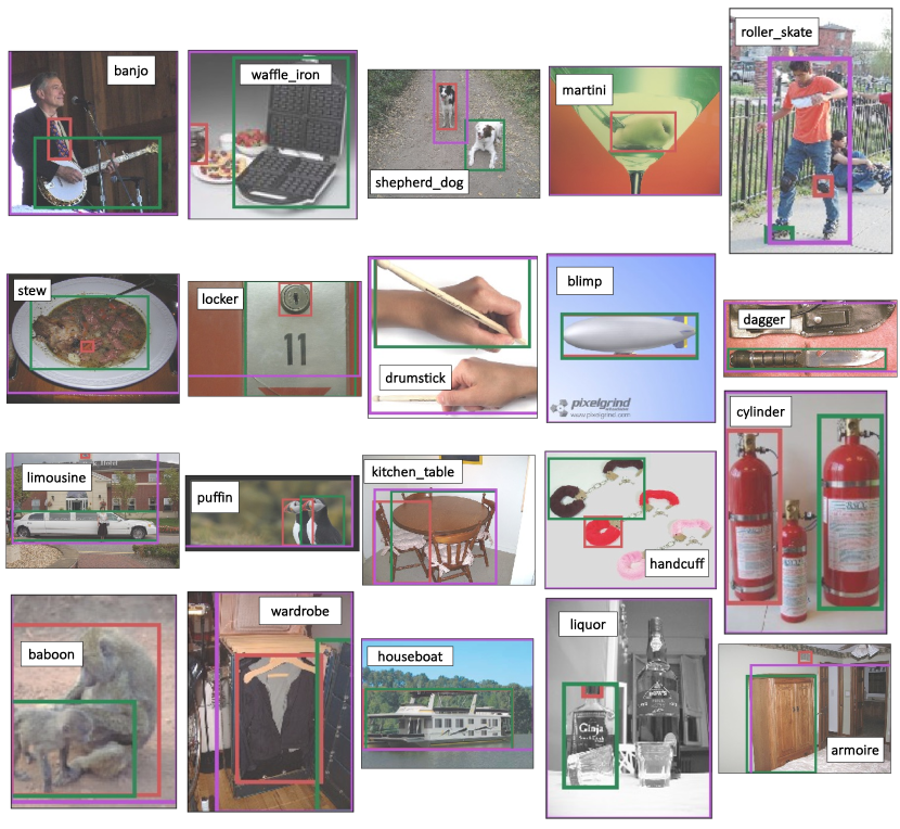
Figure 14: Random samples of prediction on unseen categories.

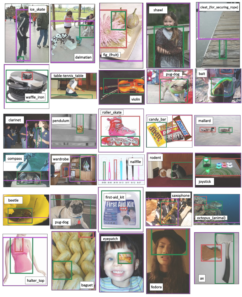
Figure 15: Random samples of prediction on unseen categories.

10 Qualitative Results

We show more visualization. Figure 14 and 15 show randomly sampled images and the pseudo-labels of decola and baseline. Images are from the ImageNet-21K from unseen categories, which none of the models are trained on. Boxes are the most confident prediction from decola and baseline and maximum size box ([74]). Green: the most confident prediction (max-score) decola trained on LVIS-base. Red: the most confident prediction (max-score) baseline trained on LVIS-base. Purple: the largest box prediction (max-size, Detic loss [74]) baseline trained on LVIS-base. All models use a Deformable DETR detector with a ResNet-50 backbone. We show randomly sampled images.

References

- Arandjelović et al. [2023] Relja Arandjelović, Alex Andonian, Arthur Mensch, Olivier J Hénaff, Jean-Baptiste Alayrac, and Andrew Zisserman. Three ways to improve feature alignment for open vocabulary detection. arXiv, 2023.
- Cai and Vasconcelos [2018] Zhaowei Cai and Nuno Vasconcelos. Cascade r-cnn: Delving into high quality object detection. In CVPR, 2018.
- Carion et al. [2020] Nicolas Carion, Francisco Massa, Gabriel Synnaeve, Nicolas Usunier, Alexander Kirillov, and Sergey Zagoruyko. End-to-end object detection with transformers. In ECCV, 2020.
- Chen et al. [2019] Kai Chen, Jiangmiao Pang, Jiaqi Wang, Yu Xiong, Xiaoxiao Li, Shuyang Sun, Wansen Feng, Ziwei Liu, Jianping Shi, Wanli Ouyang, et al. Hybrid task cascade for instance segmentation. In CVPR, 2019.
- Chen et al. [2022] Qiang Chen, Xiaokang Chen, Jian Wang, Haocheng Feng, Junyu Han, Errui Ding, Gang Zeng, and Jingdong Wang. Group detr: Fast detr training with group-wise one-to-many assignment. arXiv preprint arXiv:2207.13085, 2022.
- Chen et al. [2023] Xi Chen, Xiao Wang, Soravit Changpinyo, AJ Piergiovanni, Piotr Padlewski, Daniel Salz, Sebastian Goodman, Adam Grycner, Basil Mustafa, Lucas Beyer, Alexander Kolesnikov, Joan Puigcerver, Nan Ding, Keran Rong, Hassan Akbari, Gaurav Mishra, Linting Xue, Ashish V Thapliyal, James Bradbury, Weicheng Kuo, Mojtaba Seyedhosseini, Chao Jia, Burcu Karagol Ayan, Carlos Riquelme Ruiz, Andreas Peter Steiner, Anelia Angelova, Xiaohua Zhai, Neil Houlsby, and Radu Soricut. PaLI: A jointly-scaled multilingual language-image model. In ICLR, 2023.
- Cho and Krähenbühl [2022] Jang Hyun Cho and Philipp Krähenbühl. Long-tail detection with effective class-margins. In ECCV, 2022.
- Cho et al. [2023] Jang Hyun Cho, Philipp Krähenbühl, and Vignesh Ramanathan. Partdistillation: Learning parts from instance segmentation. In CVPR, 2023.
- Dave et al. [2021] Achal Dave, Piotr Dollár, Deva Ramanan, Alexander Kirillov, and Ross Girshick. Evaluating large-vocabulary object detectors: The devil is in the details. arXiv, 2021.
- Dehghani [2023] Mostafa et al Dehghani. Scaling vision transformers to 22 billion parameters. ICML, 2023.
- Devlin et al. [2019] Jacob Devlin, Ming-Wei Chang, Kenton Lee, and Kristina Toutanova. Bert: Pre-training of deep bidirectional transformers for language understanding. 2019.
- Du et al. [2022] Yu Du, Fangyun Wei, Zihe Zhang, Miaojing Shi, Yue Gao, and Guoqi Li. Learning to prompt for open-vocabulary object detection with vision-language model. 2022.
- Fang et al. [2023] Yuxin Fang, Wen Wang, Binhui Xie, Quan Sun, Ledell Wu, Xinggang Wang, Tiejun Huang, Xinlong Wang, and Yue Cao. Eva: Exploring the limits of masked visual representation learning at scale. In CVPR, 2023.
- Feng et al. [2022] Chengjian Feng, Yujie Zhong, Zequn Jie, Xiangxiang Chu, Haibing Ren, Xiaolin Wei, Weidi Xie, and Lin Ma. Promptdet: Towards open-vocabulary detection using uncurated images. In ECCV, 2022.
- Gadre et al. [2023] Samir Yitzhak Gadre, Gabriel Ilharco, Alex Fang, Jonathan Hayase, Georgios Smyrnis, Thao Nguyen, Ryan Marten, Mitchell Wortsman, Dhruba Ghosh, Jieyu Zhang, Eyal Orgad, Rahim Entezari, Giannis Daras, Sarah M Pratt, Vivek Ramanujan, Yonatan Bitton, Kalyani Marathe, Stephen Mussmann, Richard Vencu, Mehdi Cherti, Ranjay Krishna, Pang Wei Koh, Olga Saukh, Alexander Ratner, Shuran Song, Hannaneh Hajishirzi, Ali Farhadi, Romain Beaumont, Sewoong Oh, Alex Dimakis, Jenia Jitsev, Yair Carmon, Vaishaal Shankar, and Ludwig Schmidt. Datacomp: In search of the next generation of multimodal datasets. In Neurips (Datasets and Benchmarks Track), 2023.
- Ghiasi et al. [2021] Golnaz Ghiasi, Yin Cui, Aravind Srinivas, Rui Qian, Tsung-Yi Lin, Ekin D Cubuk, Quoc V Le, and Barret Zoph. Simple copy-paste is a strong data augmentation method for instance segmentation. In CVPR, 2021.
- Girshick [2015] Ross Girshick. Fast r-cnn. In ICCV, 2015.
- Girshick et al. [2014] Ross Girshick, Jeff Donahue, Trevor Darrell, and Jitendra Malik. Rich feature hierarchies for accurate object detection and semantic segmentation. In CVPR, 2014.
- Gu et al. [2022] Xiuye Gu, Tsung-Yi Lin, Weicheng Kuo, and Yin Cui. Open-vocabulary object detection via vision and language knowledge distillation. In ICLR, 2022.
- Gupta et al. [2019] Agrim Gupta, Piotr Dollar, and Ross Girshick. Lvis: A dataset for large vocabulary instance segmentation. In CVPR, 2019.
- He et al. [2016] Kaiming He, Xiangyu Zhang, Shaoqing Ren, and Jian Sun. Deep residual learning for image recognition. In CVPR, 2016.
- He et al. [2017] Kaiming He, Georgia Gkioxari, Piotr Dollár, and Ross Girshick. Mask r-cnn. In ICCV, 2017.
- Hinton et al. [2015] Geoffrey Hinton, Oriol Vinyals, and Jeffrey Dean. Distilling the knowledge in a neural network. In Neurips, 2015.
- Ilharco [2021] Gabriel et al Ilharco. Openclip, 2021.
- Jia et al. [2023] Ding Jia, Yuhui Yuan, Haodi He, Xiaopei Wu, Haojun Yu, Weihong Lin, Lei Sun, Chao Zhang, and Han Hu. Detrs with hybrid matching. 2023.
- Kamath et al. [2021] Aishwarya Kamath, Mannat Singh, Yann LeCun, Ishan Misra, Gabriel Synnaeve, and Nicolas Carion. Mdetr - modulated detection for end-to-end multi-modal understanding. ICCV, 2021.
- Kim et al. [2023a] Dahun Kim, Anelia Angelova, and Weicheng Kuo. Contrastive feature masking open-vocabulary vision transformer. In ICCV, 2023a.
- Kim et al. [2023b] Dahun Kim, Anelia Angelova, and Weicheng Kuo. Detection-oriented image-text pretraining for open-vocabulary detection. arXiv, 2023b.
- Kim et al. [2023c] Dahun Kim, Anelia Angelova, and Weicheng Kuo. Region-aware pretraining for open-vocabulary object detection with vision transformers. In CVPR, 2023c.
- Krishna et al. [2017] Ranjay Krishna, Yuke Zhu, Oliver Groth, Justin Johnson, Kenji Hata, Joshua Kravitz, Stephanie Chen, Yannis Kalantidis, Li-Jia Li, David A Shamma, et al. Visual genome: Connecting language and vision using crowdsourced dense image annotations. IJCV, 2017.
- Kuo et al. [2023] Weicheng Kuo, Yin Cui, Xiuye Gu, AJ Piergiovanni, and Anelia Angelova. Open-vocabulary object detection upon frozen vision and language models. In ICLR, 2023.
- Kuznetsova et al. [2020] Alina Kuznetsova, Hassan Rom, Neil Alldrin, Jasper Uijlings, Ivan Krasin, Jordi Pont-Tuset, Shahab Kamali, Stefan Popov, Matteo Malloci, Alexander Kolesnikov, et al. The open images dataset v4: Unified image classification, object detection, and visual relationship detection at scale. IJCV, 2020.
- Li et al. [2022a] Junnan Li, Dongxu Li, Caiming Xiong, and Steven Hoi. Blip: Bootstrapping language-image pre-training for unified vision-language understanding and generation. In ICML, 2022a.
- Li et al. [2022b] Liunian Harold Li, Pengchuan Zhang, Haotian Zhang, Jianwei Yang, Chunyuan Li, Yiwu Zhong, Lijuan Wang, Lu Yuan, Lei Zhang, Jenq-Neng Hwang, et al. Grounded language-image pre-training. In CVPR, 2022b.
- Lin et al. [2023] Chuang Lin, Peize Sun, Yi Jiang, Ping Luo, Lizhen Qu, Gholamreza Haffari, Zehuan Yuan, and Jianfei Cai. Learning object-language alignments for open-vocabulary object detection. In ICLR, 2023.
- Lin et al. [2014] Tsung-Yi Lin, Michael Maire, Serge Belongie, James Hays, Pietro Perona, Deva Ramanan, Piotr Dollár, and C Lawrence Zitnick. Microsoft coco: Common objects in context. In ECCV, 2014.
- Liu et al. [2022] Shilong Liu, Feng Li, Hao Zhang, Xiao Yang, Xianbiao Qi, Hang Su, Jun Zhu, and Lei Zhang. DAB-DETR: Dynamic anchor boxes are better queries for DETR. In ICLR, 2022.
- Liu et al. [2023] Shilong Liu, Zhaoyang Zeng, Tianhe Ren, Feng Li, Hao Zhang, Jie Yang, Chunyuan Li, Jianwei Yang, Hang Su, Jun Zhu, et al. Grounding dino: Marrying dino with grounded pre-training for open-set object detection. arXiv preprint arXiv:2303.05499, 2023.
- Liu et al. [2021] Ze Liu, Yutong Lin, Yue Cao, Han Hu, Yixuan Wei, Zheng Zhang, Stephen Lin, and Baining Guo. Swin transformer: Hierarchical vision transformer using shifted windows. In ICCV, 2021.
- Loshchilov and Hutter [2019] Ilya Loshchilov and Frank Hutter. Decoupled weight decay regularization. In ICLR, 2019.
- Ma et al. [2023] Chuofan Ma, Yi Jiang, Xin Wen, Zehuan Yuan, and Xiaojuan Qi. Codet: Co-occurrence guided region-word alignment for open-vocabulary object detection. In Nuerips, 2023.
- Matthias Minderer [2023] Neil Houlsby Matthias Minderer, Alexey Gritsenko. Scaling open-vocabulary object detection. NeurIPS, 2023.
- Meng et al. [2021] Depu Meng, Xiaokang Chen, Zejia Fan, Gang Zeng, Houqiang Li, Yuhui Yuan, Lei Sun, and Jingdong Wang. Conditional detr for fast training convergence. In ICCV, 2021.
- Minderer et al. [2022] Matthias Minderer et al. Simple open-vocabulary object detection with vision transformers. ECCV, 2022.
- Ouyang-Zhang et al. [2022] Jeffrey Ouyang-Zhang, Jang Hyun Cho, Xingyi Zhou, and Philipp Krähenbühl. Nms strikes back. arXiv preprint arXiv:2212.06137, 2022.
- Paszke et al. [2019] Adam Paszke, Sam Gross, Francisco Massa, Adam Lerer, James Bradbury, Gregory Chanan, Trevor Killeen, Zeming Lin, Natalia Gimelshein, Luca Antiga, Alban Desmaison, Andreas Kopf, Edward Yang, Zachary DeVito, Martin Raison, Alykhan Tejani, Sasank Chilamkurthy, Benoit Steiner, Lu Fang, Junjie Bai, and Soumith Chintala. Pytorch: An imperative style, high-performance deep learning library. In Neurips. 2019.
- Radford et al. [2021] Alec Radford, Jong Wook Kim, Chris Hallacy, Aditya Ramesh, Gabriel Goh, Sandhini Agarwal, Girish Sastry, Amanda Askell, Pamela Mishkin, Jack Clark, et al. Learning transferable visual models from natural language supervision. In ICML, 2021.
- Rasheed et al. [2022] Hanoona Abdul Rasheed, Muhammad Maaz, Muhammd Uzair Khattak, Salman Khan, and Fahad Khan. Bridging the gap between object and image-level representations for open-vocabulary detection. In Neurips, 2022.
- Ren et al. [2015] Shaoqing Ren, Kaiming He, Ross Girshick, and Jian Sun. Faster r-cnn: Towards real-time object detection with region proposal networks. Neurips, 2015.
- Ridnik et al. [2021] Tal Ridnik, Emanuel Ben-Baruch, Asaf Noy, and Lihi Zelnik. Imagenet-21k pretraining for the masses. In Neurips, 2021.
- Russakovsky et al. [2015] Olga Russakovsky, Jia Deng, Hao Su, Jonathan Krause, Sanjeev Satheesh, Sean Ma, Zhiheng Huang, Andrej Karpathy, Aditya Khosla, Michael Bernstein, Alexander C. Berg, and Li Fei-Fei. ImageNet Large Scale Visual Recognition Challenge. IJCV, 2015.
- Schuhmann et al. [2022] Christoph Schuhmann, Romain Beaumont, Richard Vencu, Cade Gordon, Ross Wightman, Mehdi Cherti, Theo Coombes, Aarush Katta, Clayton Mullis, Mitchell Wortsman, et al. Laion-5b: An open large-scale dataset for training next generation image-text models. Neurips, 2022.
- Shao et al. [2019] Shuai Shao, Zeming Li, Tianyuan Zhang, Chao Peng, Gang Yu, Xiangyu Zhang, Jing Li, and Jian Sun. Objects365: A large-scale, high-quality dataset for object detection. In ICCV, 2019.
- Sharma et al. [2018] Piyush Sharma, Nan Ding, Sebastian Goodman, and Radu Soricut. Conceptual captions: A cleaned, hypernymed, image alt-text dataset for automatic image captioning. In ACL, 2018.
- Shi and Yang [2023] Cheng Shi and Sibei Yang. Edadet: Open-vocabulary object detection using early dense alignment. In ICCV, 2023.
- Tan et al. [2020] Jingru Tan, Changbao Wang, Buyu Li, Quanquan Li, Wanli Ouyang, Changqing Yin, and Junjie Yan. Equalization loss for long-tailed object recognition. In CVPR, 2020.
- Tan et al. [2021] Jingru Tan, Xin Lu, Gang Zhang, Changqing Yin, and Quanquan Li. Equalization loss v2: A new gradient balance approach for long-tailed object detection. In CVPR, 2021.
- Wang et al. [2021] Jiaqi Wang, Wenwei Zhang, Yuhang Zang, Yuhang Cao, Jiangmiao Pang, Tao Gong, Kai Chen, Ziwei Liu, Chen Change Loy, and Dahua Lin. Seesaw loss for long-tailed instance segmentation. In CVPR, 2021.
- Wang et al. [2023] Luting Wang, Yi Liu, Penghui Du, Zihan Ding, Yue Liao, Qiaosong Qi, Biaolong Chen, and Si Liu. Object-aware distillation pyramid for open-vocabulary object detection. In CVPR, 2023.
- Wang [2023] Tao Wang. Learning to detect and segment for open vocabulary object detection. In CVPR, 2023.
- Wang et al. [2022] Yingming Wang, Xiangyu Zhang, Tong Yang, and Jian Sun. Anchor detr: Query design for transformer-based detector. In AAAI, 2022.
- Wu et al. [2023a] Size Wu, Wenwei Zhang, Sheng Jin, Wentao Liu, and Chen Change Loy. Aligning bag of regions for open-vocabulary object detection. In CVPR, 2023a.
- Wu et al. [2023b] Xiaoshi Wu, Feng Zhu, Rui Zhao, and Hongsheng Li. Cora: Adapting clip for open-vocabulary detection with region prompting and anchor pre-matching. In CVPR, 2023b.
- Wu et al. [2019] Yuxin Wu, Alexander Kirillov, Francisco Massa, Wan-Yen Lo, and Ross Girshick. Detectron2, 2019.
- Xu et al. [2023] Yifan Xu, Mengdan Zhang, Chaoyou Fu, Peixian Chen, Xiaoshan Yang, Ke Li, and Changsheng Xu. Multi-modal queried object detection in the wild. In Neurips, 2023.
- Zang et al. [2022] Yuhang Zang, Wei Li, Kaiyang Zhou, Chen Huang, and Chen Change Loy. Open-vocabulary detr with conditional matching. In ECCV, 2022.
- Zareian et al. [2021] Alireza Zareian, Kevin Dela Rosa, Derek Hao Hu, and Shih-Fu Chang. Open-vocabulary object detection using captions. In CVPR, 2021.
- Zhai et al. [2022] Xiaohua Zhai, Xiao Wang, Basil Mustafa, Andreas Steiner, Daniel Keysers, Alexander Kolesnikov, and Lucas Beyer. Lit: Zero-shot transfer with locked-image text tuning. In CVPR, 2022.
- Zhang et al. [2021] Cheng Zhang, Tai-Yu Pan, Yandong Li, Hexiang Hu, Dong Xuan, Soravit Changpinyo, Boqing Gong, and Wei-Lun Chao. MosaicOS: A simple and effective use of object-centric images for long-tailed object detection. In ICCV, 2021.
- Zhang et al. [2022] Haotian Zhang, Pengchuan Zhang, Xiaowei Hu, Yen-Chun Chen, Liunian Li, Xiyang Dai, Lijuan Wang, Lu Yuan, Jenq-Neng Hwang, and Jianfeng Gao. Glipv2: Unifying localization and vision-language understanding. Neurips, 2022.
- Zhang et al. [2023] Hao Zhang, Feng Li, Shilong Liu, Lei Zhang, Hang Su, Jun Zhu, Lionel M Ni, and Heung-Yeung Shum. Dino: Detr with improved denoising anchor boxes for end-to-end object detection. 2023.
- Zhong et al. [2022] Yiwu Zhong, Jianwei Yang, Pengchuan Zhang, Chunyuan Li, Noel Codella, Liunian Harold Li, Luowei Zhou, Xiyang Dai, Lu Yuan, Yin Li, et al. Regionclip: Region-based language-image pretraining. In CVPR, 2022.
- Zhou et al. [2021] Xingyi Zhou, Vladlen Koltun, and Philipp Krähenbühl. Probabilistic two-stage detection. arXiv preprint arXiv:2103.07461, 2021.
- Zhou et al. [2022a] Xingyi Zhou, Rohit Girdhar, Armand Joulin, Philipp Krähenbühl, and Ishan Misra. Detecting twenty-thousand classes using image-level supervision. In ECCV, 2022a.
- Zhou et al. [2022b] Xingyi Zhou, Vladlen Koltun, and Philipp Krähenbühl. Simple multi-dataset detection. In CVPR, 2022b.
- Zhu et al. [2021] Xizhou Zhu, Weijie Su, Lewei Lu, Bin Li, Xiaogang Wang, and Jifeng Dai. Deformable {detr}: Deformable transformers for end-to-end object detection. In ICLR, 2021.
- Zoph et al. [2020] Barret Zoph, Golnaz Ghiasi, Tsung-Yi Lin, Yin Cui, Hanxiao Liu, Ekin Dogus Cubuk, and Quoc Le. Rethinking pre-training and self-training. Neurips, 2020.