Measurements of the Thermal and Ionization State of the Intergalactic Medium during the Cosmic Afternoon

Abstract

We perform the first measurement of the thermal and ionization state of the intergalactic medium (IGM) across $0.9<z<1.5$ using 301 Ly$\alpha$ absorption lines fitted from 12 archival HST STIS quasar spectra, with a total pathlength of $\Delta z=2.1$. We employ the machine-learning-based inference method that uses joint Doppler parameter - column density ($b-N_{{\mbox{\scriptsize\text{H\,{i}}}}{}}$) distributions obtained from Ly$\alpha$ forest decomposition. Our results show that the H i photoionization rates, $\Gamma_{{\mbox{\scriptsize\text{H\,{i}}}}{}}$, are in good agreement with the recent UV background synthesis models, with $\log(\Gamma_{{\mbox{\scriptsize\text{H\,{i}}}}}/\text{s}^{-1})={-11.79}^{+0.18}_{-0.15}$, ${-11.98}^{+0.09}_{-0.09}$, and ${-12.32}^{+0.10}_{-0.12}$ at $z=1.4$, $1.2$, and $1$ respectively. We obtain the IGM temperature at the mean density, $T_{0}$, and the adiabatic index, $\gamma$, as $[\log(T_{0}/\text{K}),\gamma]=$ [${4.13}^{+0.12}_{-0.10}$, ${1.34}^{+0.10}_{-0.15}$], $[{3.79}^{+0.11}_{-0.11}$, ${1.70}^{+0.09}_{-0.09}]$ and $[{4.12}^{+0.15}_{-0.25}$, ${1.34}^{+0.21}_{-0.26}]$ at $z=1.4$, $1.2$ and $1$ respectively. Our measurements of $T_{0}$ at $z=1.4$ and $1.2$ are consistent with the expected trend from $z<3$ temperature measurements as well as theoretical expectations that, in the absence of any non-standard heating, the IGM should cool down after He ii reionization. Whereas, our $T_{0}$ measurements at $z=1$ show unexpectedly high IGM temperature. However, because of the relatively large uncertainty in these measurements of the order of $\Delta(T_{0})\sim 5000$ K, mostly emanating from the limited redshift path length of available data in these bins, we can not definitively conclude whether the IGM cools down at $z<1.5$. Lastly, we generate a mock dataset to test the constraining power of future measurement with larger datasets. The results demonstrate that, with redshift pathlength $\Delta z\sim 2$ for each redshift bin, three times the current dataset, we can constrain the $T_{0}$ of IGM within $1500$K. Such precision would be sufficient to conclusively constrain the history of IGM thermal evolution at $z<1.5$.

1 Introduction

After hydrogen reionization ($z<6$) (Madau et al., 1998; Fan et al., 2006; Faucher-Giguère et al., 2008; Robertson et al., 2015; McGreer et al., 2015), the thermal state of the intergalactic medium (IGM) is determined by the balance between heating from photoionization by the extragalactic UV background (UVB) and cooling mechanisms, including adiabatic cooling because of the Hubble expansion, radiative recombination cooling, and inverse Compton scattering where electrons interact with the cosmic microwave background. As a result of these processes, after the epoch of reionization, the intergalactic medium (IGM) subsequently adheres to the power-law temperature-density ($T$-$\Delta$) relation:

$$T(\Delta)=T_{0}\Delta^{\gamma-1},$$ (1)

where $\Delta=\rho/\bar{\rho}$ is the overdensity, $T_{0}$ is the temperature at mean density $\bar{\rho}$, and $\gamma$ is the power-law index (Hui & Gnedin, 1997; McQuinn & Upton Sanderbeck, 2016). These two parameters $[T_{0},\gamma]$ thus characterize the thermal state of the IGM, and enable us to impose constraints on its thermal history at various epochs (Davé & Tripp, 2001; Becker et al., 2011; Rorai et al., 2017; Hiss et al., 2018; Gaikwad et al., 2021), which enhance our understanding of the IGM thermal evolution and illustrate the intrinsic heating and cooling mechanisms of the Universe.

Based on current theoretical models, by the later stages of the universe ($z\lesssim 1.7$), i.e. long after the end of helium reionization at $z\sim 3$ (McQuinn et al., 2009; Worseck et al., 2011; Khaire, 2017), the thermal state of the IGM is dominated by the adiabatic cooling driven by Hubble expansion. Consequently, it is predicted that the IGM cools to temperatures around $T_{0}\sim 5000$ K and $\gamma\sim 1.6$ by $z\sim 0$ (McQuinn & Upton Sanderbeck, 2016). Interestingly, the specifics of He ii reionization hardly influence this outcome (Oñorbe et al., 2017b, a). This is because, after roughly 200 Myr, the IGM essentially "forgets" its past thermal history due to the aforementioned adiabatic cooling. Standard hydrodynamical simulations routinely forecast this cooling pattern of the IGM to temperatures of $T_{0}\sim 5000$ K by $z\sim 0$, however, there is not enough observational evidence to confirm this claim. This is mainly because of the large scatter in the $T_{0}$ measurements performed using various techniques over the last two decades at $1.7<z<3$, although most recent measurement (Hiss et al., 2018; Walther et al., 2019a; Gaikwad et al., 2021) hint towards cooling down of the IGM at $z<3$. The most conclusive evidence of the cooling of the IGM should come from the $T_{0}$ measurements at $z<1.5$ however these measurements are challenging. Part of the challenge lies in the fact that for $z\lesssim 1.7$, the Ly$\alpha$ transition is obstructed by the atmospheric cutoff ($\lambda\sim 3300$ Å), necessitating UV space observations via Hubble Space Telescope (HST), the only space-based telescope that has FUV and NUV spectrographs capable of providing data for these measurements. Currently, the only measurements of the IGM thermal state for $z<1.7$ come from Ricotti et al. (2000) and Davé & Tripp (2001), both utilizing datasets with very limited size ($\sim$ 50 Ly$\alpha$ absorption lines). Due to the limited scale of this dataset, the associated error margins are substantial, with $\sigma_{T_{0}}\gtrsim$ 5000K. This limitation implies that our understanding of the IGM therm state at low-$z$ remains imprecise.

Recent analyses of Hubble Space Telescope (HST) Cosmic Origins Spectrograph (COS) Ly$\alpha$ absorption spectra at $z<0.5$ suggest that the IGM temperature at low-$z$ may exceed theoretical predictions (Gaikwad et al., 2017b; Viel et al., 2017; Nasir et al., 2017). This claim stems from the decomposition of Ly$\alpha$ lines, where each line is characterized by its Doppler parameter $b$ and the neutral hydrogen column density $N_{\rm HI}$. These studies show that the low-$z$ Ly$\alpha$ lines appear notably broader than anticipated, indicated by larger $b$-parameters compared with those obtained from hydro simulations with and without feedback (Bolton et al., 2022b; Hu et al., 2023; Khaire et al., 2023a). Since these hydro simulations model the low-density gas traced by the Ly$\alpha$ forest, from the first principles, the most straightforward interpretation for these enlarged $b$ values is thermal broadening, suggesting an unexpectedly high IGM temperature (Viel et al., 2017) or non-standard missing turbulence in the simulations (Gaikwad et al., 2017b; Bolton et al., 2022b). If the IGM temperature is indeed higher than current models predict, it necessitates a reconsideration of heating sources. Potential mechanisms might include feedback effects from galaxy formation processes (however see Khaire et al., 2023a, b; Hu et al., 2023) or more novel phenomena such as heating due to dark matter annihilation (Bolton et al., 2022a). Additionally, turbulent broadening from non-gravitational forces, which are not yet integrated into simulations, could also play a role (Gaikwad et al., 2017b; Bolton et al., 2022b). It is noteworthy that this discrepancy in $b$ parameter distributions is found only in low-$z$. In contrast, at $z\gtrsim 2$, the distribution of $b$ parameters aligns well with the predictions made by hydro simulations regarding thermal and turbulent broadening (e.g Bolton et al., 2014; Hiss et al., 2019).

In addition to the discrepancy in $b$ parameters, the low-$z$ IGM presents another puzzle: the nature of the UV background (UVB), characterized by the H i photoionization rate, $\Gamma_{{\mbox{\scriptsize\text{H\,{i}}}}{}}$, which directly affects the abundance of Ly$\alpha$ absorbers in the low-$z$ IGM as well as crucial for studying the circum-galactic medium (e.g Lehner et al., 2013; Hussain et al., 2017; Chen et al., 2017; Wotta et al., 2019; Acharya & Khaire, 2022). A notable deviation between the $\Gamma_{{\mbox{\scriptsize\text{H\,{i}}}}{}}$ deduced from the Ly$\alpha$ forest at $z\sim 0.1$ and the forecasts from previous UVB synthesis models (e.g Haardt & Madau, 2012; Faucher-Giguère et al., 2009) lead Kollmeier et al. (2014) to introduce the problem of a "photon under-production crisis", which has however not been confirmed by other studies (Shull et al., 2015; Gaikwad et al., 2017a; Fumagalli et al., 2017; Khaire et al., 2019) and recent UVB models (Khaire & Srianand, 2015, 2019; Puchwein et al., 2019; Faucher-Giguère, 2020). The recent UVB models agree to the extent that the low-z $\Gamma_{{\mbox{\scriptsize\text{H\,{i}}}}{}}$ measurements favour UVB dominated by H i ionizing photons from quasars alone and the fraction of ionizing photons from galaxies at $z<2$ is negligibly small (Khaire & Srianand, 2019; Puchwein et al., 2019; Faucher-Giguère, 2020). However, at higher redshifts, $z>3$, a substantial increase in the ionizing escape fraction from galaxies from less than one percent to 15-20 percent is needed (Khaire et al., 2016) even in the presence of a high fraction of low-luminosity quasars claimed to be present at high-$z$ (Khaire, 2017; Finkelstein et al., 2019). This transition of escape fraction hinges only on the $\Gamma_{{\mbox{\scriptsize\text{H\,{i}}}}{}}$ measurements at $z>2$ and $z<0.5$ whereas there are no measurement of $\Gamma_{{\mbox{\scriptsize\text{H\,{i}}}}{}}$ at $0.5<z<1.8$, with a substantial void of almost five billion years of cosmic time. A part of this lack of measurement, besides the limited data from HST at these redshifts, is caused by the potential degeneracy between the IGM thermal and ionization states. To overcome this for $z<0.5$ $\Gamma_{{\mbox{\scriptsize\text{H\,{i}}}}{}}$ measurements previous studies (Gaikwad et al., 2017a; Khaire et al., 2019) leveraged either post-processing simulations to generate the thermal histories (Gaikwad et al., 2018) or a huge grid of NyX simulations (Walther et al., 2017) performed with different thermal histories of the IGM. It is important to recognize, a full description of the Ly$\alpha$ forest depends on three parameters $T_{0}$, $\gamma$, and $\Gamma_{{\mbox{\scriptsize\text{H\,{i}}}}{}}$. Degeneracies among these variables require that any reliable data-model comparison must adopt a careful statistical inference procedure.

To overcome the aforementioned difficulties, Hu et al. (2022, hereafter Hu22) adopts an inference method which jointly measures the thermal and ionization state of the low-$z$ IGM based on the decomposition of the Ly$\alpha$ forest into Doppler broadening parameter $b$ and column density $N_{{\mbox{\scriptsize\text{H\,{i}}}}{}}$. In this framework, Bayesian inference of the model parameters [$\log T_{0}$, $\gamma$, $\log\Gamma_{{\mbox{\scriptsize\text{H\,{i}}}}{}}$] is conducted based on the 2D joint $b$-$N_{{\mbox{\scriptsize\text{H\,{i}}}}{}}$ distribution and the line density d$N$/d$z$, with the help of neural density estimators (Alsing et al., 2019) and Gaussian emulators (Ambikasaran et al., 2016), both trained on a suite of Nyx simulations consisting of 51 simulation models with different thermal histories (Walther et al., 2017; Hiss et al., 2018). Such an inference method enables us to measure the thermal and ionization state of the IGM to high precision using limited-sized data.

In this work, we employ the aforementioned method to measure both the thermal and ionization state of the IGM using quasar spectra obtained from Space Telescope Imaging Spectrograph (STIS) on board HST. We opt for STIS due to its superior resolution compared with COS and available archival data. We utilize 12 HST STIS quasar spectra covering $0.9<z<1.5$, which are selected from the STIS archive based on their redshift coverage, signal-to-noise ratio (SNR)s, and the availability of metal identification. For the identification of metal lines, we import the metal identification from the COS Absorption Survey of Baryon Harbors (CASBaH) project (Tripp, 2014; Prochaska et al., 2019; Burchett et al., 2019; Haislmaier et al., 2021) for five of our spectra, and make use of the metal identification from Milutinović et al. (2007) for the remaining seven spectra. We fit these spectra to obtain our $\left\{b,N_{{\mbox{\scriptsize\text{H\,{i}}}}{}}\right\}$ sample using VPFIT (see § 2.1) and apply the Hu22 method to measure the thermal and ionization state of the IGM in three redshift bins centering on $z=1$, 1.2, and 1.4.

This paper is structured as follows. We introduce our observational data in § 2 together with the data processing procedure, including continuum fitting, Voigt profiles fitting, and metal masking. In §3 we describe our hydrodynamic simulations, parameter grid, and mock data processing procedures, including generating Ly$\alpha$ forest from simulation, creating mock sightlines, and forward-modeling. In §4 we present our inference algorithm, including emulators and likelihood function. Afterwards, we discuss our results in §6. In the end, we summarize the highlights of this study in §7. Throughout this paper, we write $\log$ in place of $\log_{10}$. Cosmology parameters used in this study ($\Omega_{m}=0.319181,\Omega_{b}h^{2}=0.022312,h=0.670386,n_{s}=0.96,\sigma_{8}=0.8288$) are taken from Planck Collaboration et al. (2014).

2 Observational Data

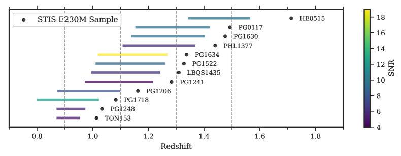
Figure 1: The HST STIS E230 spectra used in this study. The quasar are shown as black dots, and the Ly$\alpha$ spectra, with proximity zones removed, are shown as line segments with their colour indicating the mean SNR (per pixel). The three redshift bins used in this study are shown by the vertical dashed lines.

To measure the thermal state of the IGM around z $\sim 1$, we make use of the quasar spectra observed with the HST STIS (Woodgate et al., 1998) using the E230M echelle mode, which provide spectroscopic coverage from $\sim$ 1600 Å to 3100 Å. We select such echelle mode for two reasons. First, as discussed in § 1, its high spectral resolution is beneficial for our analysis, with R $\sim$ 30,000, corresponding to $\sim 10\text{ km/s}$ (Kimble et al., 1998; Medallon & Welty, 2023), and its line spread function (LSF) is close to Gaussian and has a weak dependence on the wavelength, which makes both the Voigt profile fitting (see § 2.1) and the generation of forward models easier (see § 3.3). Secondly, the echelle modes have higher wavelength coverage compared with first-order grating modes, enabling us to measure the $\left\{b,N_{{\mbox{\scriptsize\text{H\,{i}}}}{}}\right\}$ of the Ly$\alpha$ absorption lines across a wider redshift range with constant instrumental effects such as LSF, which makes our analysis across different redshift bins more robust. We search the archival HST STIS E230M data observed in the 0.2” × 0.2” slit, and retrieve 12 spectra with average SNR $\gtrsim 5$. The details of the observation, from which our quasar samples are obtained, are summarized in Table 1, and Fig. 1 depicts the redshift coverage of the spectra used in this study. The quasars are shown as black dots, and the spectra are shown as line segments with their colour indicating the SNR. The redshift bins considered for the measurements are shown by the vertical dashed lines in Fig. 1.

To reduce and combine the STIS spectra, we used the procedure of Tripp et al. (2001) with CALSTIS v3.4.2. In brief, starting with the CALSTIS x1d files, for each quasar we combined all exposures, including the coaddition of overlapping regions of adjacent echelle orders, all with appropriate weighting and using the STIS flags to mask out bad pixels (see Tripp et al., 2001, for details). We then fit the continuum of these spectra using the interactive continuum fitting program imported from linetools. Since we focus on the Ly$\alpha$ forest in this study, we make use of only the Ly$\alpha$ regions, excluding Ly$\beta$ and higher Lyman series absorption lines at $\lambda<1050$ Å, while also masking the quasar proximity zones at $\lambda>1180$ Å (see Fig.1). As a result, we only use the spectral segment with rest frame wavelength $1050<\lambda_{\text{rest}}<1180$ Å. The quasar sightlines are chopped and padded by white noise based on the noise vector of the spectrum before passing into the VP-fitting program to avoid any complications arising from the edges of the spectra, and the padded regions are later masked in post-processing. Such a treatment to the edges is also applied to the mock forward models to ensure our analysis is consistent.

Table 1: Summary of HST STIS observations used in the study

ID	$z_{qso}$	STIS wavelength range	Obs date	Exp time	average SNR/pix	average SNR/pix
		(Å)		(ksec)	(full spectra)	(Ly$\alpha$ regions)
TON153	1.014	2275 - 3110	2001 Jan.	5.3	5.0	4.8
			2002 Jun.	8.2
PG1248+401	1.033	2275 - 3110	2002 Jul.	25.2	5.9	5.0
			2001 Oct.	28.8
PG1718+481	1.083	1841 - 2673	1999 Nov.	14.1	7.9	9.8
PG1206+459a	1.162	2273 - 3110	2001 Jan.	17.3	7.3	6.4
LBQS1435-0134a	1.309	1985 - 2781	2015 Jun.	20.9	10.6	5.5
PG1241+176	1.283	2275 - 3110	2002 Jun.	19.2	4.7	4.4
PG1522+101a	1.328	1985 - 2781	2015 Mar.	7.7	9.5	7.1
			2015 May.	13.2
PG1634+706	1.337	1858 - 2673	1999 May.	14.5	12.9	18.7
		2275 - 3110	1999 Jun.	14.5
		1858 - 2673	1999 Jun.	26.4
PHL1377a	1.440	2275 - 3110	2002 Jan.	14.0	7.2	5.3
			2002 Feb.	28.0
PG1630+377a	1.476	2275 - 3110	2001 Feb.	5.3	10.6	7.5
			2001 Oct.	28.8
PG0117+213	1.493	2275 - 3110	2000 Dec.	42.0	7.2	7.5
HE0515-4414	1.713	2275 - 3110	2000 Jan.	31.5	7.9	7.6

• ^a The quasar sightlines on which we use the metal identification from the COS Absorption Survey of Baryon Harbors (CASBaH).

2.1 Voigt-Profile Fitting

In this work, we use the line-fitting program VPFIT, which fits a collection of Voigt profiles convolved with the instrument LSF to spectroscopic data (Carswell & Webb, 2014). We employ a fully automated VPFIT python wrapper adapted from Hiss et al. (2018), which is built on the VPFIT version 11.1. The wrapper routine controls VPFIT with the help of the VPFIT front-end/back-end programs RDGEN and AUTOVPIN and fit our simulated spectra automatically. We set up VPFIT to explore the range of parameters $1\leq b\leq 300~{}\text{km/s}$ and $11.5\leq\log(N_{{\mbox{\scriptsize\text{H\,{i}}}}}/\text{cm}^{-2})\leq 18$ for every single Ly$\alpha$ absorption lines. VPFIT automatically varies these parameters and fits for additional component lines until the $\chi^{2}$ with respect to the whole spectral segment is minimized. Such a VP-fitting procedure is applied to the whole spectral segment, fitting both the Ly$\alpha$ lines and metal lines, including both intervening metal lines and those from interstellar medium of Milky Way (MW); for simplicity, hereafter we refer to these collectively as metal lines. The removal of these metal lines is later discussed in § 2.2.

During our VP-fitting procedure, we noticed the presence of artefacts in the spectra, which are absent in our simulated and forward-modelled mock datasets. A visual assessment of these minor features in the data suggested they were not genuine, but rather artefacts from factors like flat fielding, continuum placement, or data reduction artifacts. This is especially true for top-quality spectra, where the exceptionally high SNR technically requires the inclusion of such faint components. To this end, we incorporate a fixed ’floor’ of 0.02 in quadrature to the normalized flux error vector for all spectra. We do this without introducing extra noise to the normalized flux. This value was determined through a process of trial and error. It was informed by the detection of a considerable number of absorption lines with notably low Doppler parameters and column densities, as reported by VPFIT in the spectra with the highest SNR. These faint, narrow lines were not observed in our simulated and forward-modelled sightlines. Nevertheless, implementing this noise floor primarily affects lines with $\log N_{{\mbox{\scriptsize\text{H\,{i}}}}{}}{}/\text{cm}^{-2}<12.5$ from our dataset, which will not be used for inference. This same noise floor is also applied to the simulated datasets to keep our data processing procedure consistent (see § 3.3).

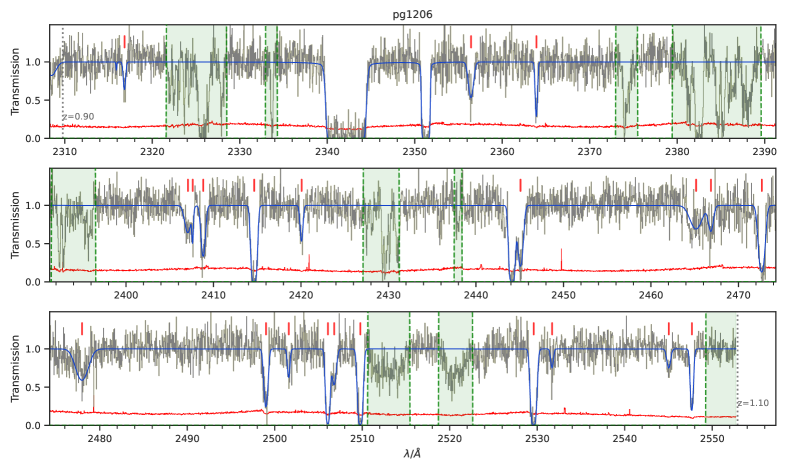
Figure 2: Illustration of the processed STIS spectrum of PG1206+459. The original spectrum is shown in gray, while a model spectrum based on VP-fitting is shown in blue. The noise vector is shown in red, and the masked regions are shown as green shaded regions. The Ly$\alpha$ lines used for our $\left\{b,N_{{\mbox{\scriptsize\text{H\,{i}}}}{}}\right\}$ dataset are labelled by red vertical lines.

Our VPFIT wrapper is designed to fit spectra using a custom LSF. However, it is important to note that it accommodates only a single LSF, without accounting for any wavelength dependency. To address this, we extract the STIS E230M LSF from linetools and interpolate it to match the central wavelength of the spectrum we aim to fit. As previously detailed in § 2, the STIS 230M exhibits a Gaussian-like LSF, which shows minimal variation across different wavelengths. Consequently, our approach of employing a singular LSF in the VP-fitting process does not introduce significant errors. To ensure consistency and avoid statistical biases, we apply the same fitting methodology to both our observational data and forward-modelled mock.

Furthermore, we follow the convention used in previous studies (Schaye et al., 2000; Rudie et al., 2012a; Hiss et al., 2018) and apply another filter for both $b$ and $N_{{\mbox{\scriptsize\text{H\,{i}}}}}$ in this study, using only $b$-$N_{{\mbox{\scriptsize\text{H\,{i}}}}}$ pairs in region $12.5\leq\log(N_{{\mbox{\scriptsize\text{H\,{i}}}}}/\text{cm}^{-2})\leq 14.5$ and $0.5\leq\log(b/\text{km s}^{-1})\leq 2.5$ in our analysis. Such a limitation is chosen to include the $b$-$N_{{\mbox{\scriptsize\text{H\,{i}}}}{}}$ distributions for all our Nyx simulation models (see § 3.1) while guaranteeing that the absorption lines are not strongly saturated, which maximizes the sensitivity to IGM thermal state and minimizes the impact of poorly understood strong absorption lines arising mainly from the circumgalactic medium of intervening galaxies.

One of our STIS spectra, PG1206 is shown as an example of the VP-fitting procedure in Fig. 2. The original spectrum is shown in grey, and the model based on VP-fitting is shown in blue. The noise vector of the original spectrum is shown in red, and the masked regions due to metal line detection are shown as green shaded regions. The Ly$\alpha$ lines used for our $\left\{b,N_{{\mbox{\scriptsize\text{H\,{i}}}}{}}\right\}$ dataset (after all filters) are labelled by red vertical lines.

2.2 Metal Identification

As previously mentioned, our VP-fitting procedure fits all absorption lines including Ly$\alpha$ lines and metal lines. For our analysis based on the $\left\{b,N_{{\mbox{\scriptsize\text{H\,{i}}}}{}}\right\}$ of the Ly$\alpha$ forest, it is critical to filter out these metal lines. To this end, we make use of archival metal identification data presented in Milutinović et al. (2007) for seven of our quasar sightlines and use metal identification from the CASBaH survey (Tripp, 2014; Prochaska et al., 2019; Burchett et al., 2019; Haislmaier et al., 2021) for the rest five spectra (see notes of the Table. 1). For each spectrum, we create a mask to cover the vicinity of each metal line based on the aforementioned metal identification. These masked regions are initially aligned with the central wavelength of the metal lines reported in the literature, while their initial widths are set to be $\Delta v=30$ km/s in velocity space. Such a value is chosen based on the resolution of STIS E230M, which corresponds to $\sim 10$ km/s. We then apply the masks to our VP-fit results to filter out potential metal lines. To do so, we first locate the absorption line region characterized by $F_{\text{line,fit}}\leq$ 0.99, where the $F_{\text{line,fit}}$ stands for the normalized flux given by the VP-fit model (the blue line in Fig. 2). If any absorption line region overlaps with the initial mask, we increase the width of the mask to cover the detected line, while the increment is given by the full width at half maximum (FWHM) of the detected line, approximated by FWHM = $b$/0.6, where the $b$ is given by VPFIT. Lastly, we adjust the masks manually to fill the small gaps (with $\Delta v=30$ km/s) between the masked regions and make sure all absorption lines close to (the original) metal masks reported by our VP-fitting procedure are masked. The aforementioned masking procedure is needed based on the fact that our VP-fitting procedure does not match the line identified in the literature exactly, due to the different spectra used for metal identification and different post-processing procedures, including coaddition, continuum fitting, and data smoothing used in our data. The aforementioned masking procedure makes sure that all potential metal contamination is removed. Afterwards, we manually masked a few gap regions in our quasar spectra resulting in the failure of the VPFIT caused by Damped Ly$\alpha$ absorption systems (DLAs). These masks are generated in post-processing, which means that we first apply VPFIT to the spectra assuming all lines are H i Ly$\alpha$ and remove the absorption lines that fall within the masked regions, same as done for finding overlapped lines with metal masks. In the end, we subtract the metal mask from our total pathlength and obtain $\Delta z=$2.097. Our full sample of quasar segments and their corresponding masks are presented in Appendix A.

With our imposed cuts on the $\left\{b,N_{{\mbox{\scriptsize\text{H\,{i}}}}{}}\right\}$, we find that 40 out of 341 lines are masked for our whole sample, and that leaves us with a $\left\{b,N_{{\mbox{\scriptsize\text{H\,{i}}}}{}}\right\}$ dataset consisting of 301 Ly$\alpha$ absorption lines. We divide the 301 Ly$\alpha$ absorbers into three redshift bins: $0.9<z<1.1$, $1.1<z<1.3$ and $1.3<z<1.5$ centered at $z=1$, $1.2$ and $1.4$, respectively, according to their central wavelength as determined by VPFIT. This provides us with the number of Ly$\alpha$ lines to be 102, 160 and 39 and redshift path of 0.762, 0.972 and 0.363 in the bins centred at $z=1$, $1.2$ and $1.4$, respectively. In Table 2 we summarize our $\left\{b,N_{{\mbox{\scriptsize\text{H\,{i}}}}{}}\right\}$ dataset for each redshift bin, with redshift pathlength, number of final Ly$\alpha$ lines as well as median values for the $b$ and $N_{{\mbox{\scriptsize\text{H\,{i}}}}}$ in each bin.

Table 2: Summary of the of the observational dataset

$z$ bins	$\Delta z$	Number	$b_{\text{m}}/\text{km s}^{-1}$	$\log(N_{{{\mbox{\scriptsize\text{H\,{i}}}}},\text{m}}/\text{cm}^{-2})$
$0.9\leq z\leq 1.1$	0.762	102	31.74	13.48
$1.1<z\leq 1.3$	0.972	160	28.83	13.37
$1.3<z\leq 1.5$	0.363	39	29.69	13.48

• The numbers of identified Ly$\alpha$ lines in each redshift, the total pathlength $\Delta z$, and the median value $b_{\text{m}}$ and $\log N_{{{\mbox{\scriptsize\text{H\,{i}}}}},\text{m}}$.

3 Simulations

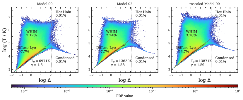
Figure 3: Volume weighted $T$-$\Delta$ distribution for three simulations models at $z=1.0$. The left panel is the Nyx model 00 with $T_{0}=6971$ K, $\gamma=1.60$, and the middle panel is the Nyx model 02 with $T_{0}=13630$ K, $\gamma=1.58$. The right panel shows the model generated by multiplying the temperature in model 00 by two, resulting in a $T_{0}=13871$ K and $\gamma=$1.59 according to our $\Delta-T$ fitting procedure. The best-fit power-law relationship is shown as grey dashed lines. The $\log T$ for each bin are plotted as black dots, with the 1-$\sigma_{T}$ error bars shown as black bars. The volume-weighted gas phase fractions are shown in the annotations. The fraction of diffuse Ly$\alpha$ gas and the values of $T_{0}$ and $\gamma$ in the rescaled model (the right panel) agree within a percent level to the actual model shown in the middle panel.

We utilize a set of Nyx cosmological hydrodynamic simulations (see Lukić et al., 2015; Almgren et al., 2013) to model the low-redshift IGM. Developed primarily for simulating the IGM, Nyx is a massively parallel cosmological simulation code. Within Nyx, dark matter evolution is captured by treating it as self-gravitating Lagrangian particles. In contrast, baryons are represented as an ideal gas on a uniform Cartesian grid, modelled using an Eulerian approach. The Eulerian gas dynamics equations are addressed using a second-order piece-wise parabolic method, ensuring accurate shock wave representation.

Nyx includes the main physical processes relevant for modelling the Ly$\alpha$ forest. Nyx assumes the gas to have a primordial composition: a hydrogen mass fraction of 0.76, a helium mass fraction of 0.24, and zero metallicity. The various processes, such as recombination, collisional ionization, dielectric recombination, and cooling, are implemented according to the methodologies described in Lukić et al. (2015). Nyx also models the process of inverse Compton cooling against the cosmic microwave background, and tracks the total thermal energy loss resulting from atomic collisional processes. The default model of NyX uses spatially uniform UVB form Haardt & Madau (2012). In subsequent stages, while generating the Ly$\alpha$ forest in post-processing (See §3.2), the UVB is treated as a variable parameter. Notably, since the Nyx simulations are tailored to study the IGM, they do not incorporate feedback or galaxy formation processes. This omission considerably reduces computational demands, enabling us to execute a vast ensemble of simulations with varied thermal parameters (as detailed in 3.1).

In this study, each Nyx simulation starts at $z=159$ and runs until $z=0.03$. It spans a simulation domain of $L_{\text{box}}=20~{}{\rm cMpc}/h$ having $N_{\text{cell}}=1024^{3}$ Eulerian cells for baryon and equal count of dark matter particles. The chosen box size strikes a balance between managing computational resources and ensuring convergence to within a margin of $<10\%$ on small scales (reflected in large $k$ values). A more detailed discussion on resolution and box size considerations can be found in Lukić et al. (2015).

Due to the inherent degeneracy between the thermal and ionization states of the IGM, it is essential to employ a substantial collection of Nyx simulations, each representing varied thermal histories. We provide a detailed description of the simulation grid utilized in this study in the following section.

3.1 Thermal Parameters and Simulation Grid

3.1.1 The THERMAL suite

To represent the IGM with varied thermal state spanning $0.9<z<1.5$, we utilize a subset of the Thermal History and Evolution in Reionization Models of Absorption Lines (THERMAL) suite of Nyx simulations (also see Hiss et al., 2018; Walther et al., 2019b). From this suite, we use 51 models, each showcasing different thermal histories. For every model, we produce three simulation snapshots at $z=1.0,1.2$, and 1.4. From these, we determine the thermal state, characterized by [$\log T_{0}$,$\gamma$]. Varied thermal histories are realized by manually adjusting the photoheating rates ($\epsilon$), in accordance with the methodology set forth in Becker et al. (2011). In this method, $\epsilon$ is treated as a function of overdensity, i.e.

$$\epsilon=A\epsilon_{\rm HM12}\Delta^{B},$$ (2)

where $\epsilon_{\rm HM12}$ represents the photoheating rate per H ii ion, tabulated in Haardt & Madau (2012), and $A$ and $B$ are parameters used to generate models with different thermal histories.

As the universe evolves towards lower redshifts, the thermal state of the IGM tends to stabilize, making it a challenge to produce models with uniformly distributed $T_{0}$ and $\gamma$ values. For an in-depth discussion on this, refer to Walther et al. 2019b. Specifically, crafting models with a low $T_{0}(<10^{3.5}~{}{\rm K})$ paired with a high $\gamma$ value $(>1.9)$ at lower redshifts proves particularly daunting. When lowering the $T_{0}$ by decreasing the photoheating rates, the cooling resulting from the Hubble expansion starts to play a dominant role, causing $\gamma$ to gravitate towards a value close to 1.6 (as discussed in McQuinn & Upton Sanderbeck, 2016). Consequently, the grid representing the interplay between $T_{0}$ and $\gamma$ assumes an irregular shape, leaving voids in regions characterized by high $\gamma$ and low $T_{0}$. This irregularity also stems from the inherent design of the parameter grid in the THERMAL suite, which can be traced back to the thermal state analysis of higher redshifts (Walther et al., 2019b).

3.1.2 $T_{0}$-rescaling models

As will be discussed later in § 5, our data favour models with high $T_{0}$ at $z=1.0$ and $z=1.4$, which is hard to generate based on the aforementioned procedure. This is because, as suggested by Eq. 2, our method alters the IGM thermal history of the simulation model by varying the heat released by the H i photoionization. However, the results of such a heating procedure fade away in low $z$, where the IGM is dominated by the adiabatic cooling caused by Hubble expansion (McQuinn, 2016). As a result, the $T_{0}$ of the IGM at $z<1.5$ becomes insensitive to the heat input in our method for models with high $T_{0}$. To this end, we rescale the IGM temperature to model the IGM with high temperature. For $z=1.0$, we select six simulation snapshots with 3.75 $\leq\log T_{0}\leq$ 3.9, which has $T_{0}$ close to the Nyx model 00 with $A=1,B=0$ (see Eq. 2) at $z=1.0$, and multiply their temperature $T$ (at each simulation cell) by 2.5 and 3 respectively to generate 12 new models. The other properties of the simulation remain unchanged, and since we rescaled the temperature of all simulation cells uniformly the whole $\Delta$-$T$ distribution of the simulation model still follows the power law $\Delta$-$T$ relationship Eq. 1 with the $T_{0}$ rescaled. The [$T_{0}$, $\gamma$] of original models and models with rescaled $T_{0}$ are illustrated in Fig. 7, where the original models are shown as green dots, the model rescaled to $2.5\times T_{0}$ and $3.0\times T_{0}$ are shown in orange and red respectively. Such temperature rescaling procedures are also applied to $z=1.4$ models, where our preliminary results also favour hot models, and the corresponding models are shown in Fig. 5.

3.1.3 Measuring the IGM thermal state $[T_{0},\gamma]$

To measure the thermal state for each of the 51 models, we fit temperature-density ($T$-$\Delta$) relation (see Eq. 1) to the temperatures and densities in the simulation domain. While fitting the $T$-$\Delta$ relationship, we noticed broader distributions of the IGM temperatures in low redshift ($z\lesssim 1.0$) compared to high redshift ($z>3$). To accommodate the dispersion in the IGM $T$-$\Delta$ distribution while fitting the power-law relationship, we adopt the fitting approach detailed in Hu22. This method first segregates the diffuse Ly$\alpha$ gas ( $T<10^{5}$K and $\Delta<120$, see Davé et al., 2010) into 20 bins based on $\log\Delta$. A linear least squares fit is then applied to the average temperatures within each bin. For this study, we’ve adjusted the fitting range to $-0.5<\log\Delta<1.5$. Examples of the $\Delta-T$ distribution and the corresponding power law fitting are shown in Fig. 3. For each panel, the best-fit power-law relationship is shown as grey dashed lines, and the $\log T$ for each bin are plotted as black dots, and the 1-$\sigma_{T}$ error bars are shown as black bars. The left panel shows the Nyx model 00 with $T_{0}=6971$ K, $\gamma=1.60$, and the middle panel shows the Nyx model 02 with $T_{0}=13630$ K, $\gamma=1.58$ generated by varying the parameter $A$ and $B$ in Eq. 2. The right panel shows the rescaled model 00 generated by multiplying the temperature in model 00 by two. It exhibit a $T_{0}=13871$ K and $\gamma=$1.59 according to our $\Delta-T$ fitting procedure.

3.1.4 Varying the UVB $\Gamma_{{\mbox{\scriptsize\text{H\,{i}}}}{}}$

Since we want to measure the ionization state of the IGM, we let the H i photoionization rate $\Gamma_{{\mbox{\scriptsize\text{H\,{i}}}}{}}$ be a free parameter when generating Ly$\alpha$ forest skewers from our simulations. As such, we add an additional parameter $\log\Gamma_{{\mbox{\scriptsize\text{H\,{i}}}}{}}$ to our thermal grid, extending it to [$\log T_{0}$, $\gamma$, $\log\Gamma_{{\mbox{\scriptsize\text{H\,{i}}}}{}}$]. Such procedure is done in the post-processing of the simulation, at the time when the simulated slightlines are generated (see § 3.2). The value of $\Gamma_{{\mbox{\scriptsize\text{H\,{i}}}}{}}$ we used in this study spans from $\log(\Gamma_{{\mbox{\scriptsize\text{H\,{i}}}}{}}/\text{s}^{-1})$ = -11.2 to -12.8 in logarithmic steps of $0.2$ dex, which gives 9 values in total. These values are fixed for all redshift bins.

3.2 Skewers

In this study, we produce mock Ly$\alpha$ spectra by calculating the Ly$\alpha$ optical depth ($\tau$) along lines of sight, referred to as skewers for simplicity. Within each simulation model, we create a set of 15,000 skewers, aligned with the $x$, $y$, and $z$ axes of the simulation box, distributing 5,000 skewers per axis. Properties necessary for the optical depth calculation are then extracted from each cell along these skewers. These properties include the temperature ($T$), overdensity ($\Delta$), and the line-of-sight velocity ($v_{z}$). Additionally, the hydrogen neutral fraction ($x_{{\mbox{\scriptsize\text{H\,{i}}}}{}}$), crucial for synthesizing Ly$\alpha$ forest skewers, is determined by assuming ionization equilibrium. This calculation incorporates both collisional ionization, dictated by the gas temperature ($T$), and photoionization. In our approach, $\Gamma_{{\mbox{\scriptsize\text{H\,{i}}}}{}}$ is treated as a free parameter during the post-processing. Considering that Nyx does not simulate radiative transfer, we employ an approximation to model the self-shielding effect of the UV background in optically thick gas. Following the method outlined by Rahmati et al. (2013), this involves attenuating $\Gamma_{{\mbox{\scriptsize\text{H\,{i}}}}{}}$ in cells with dense gas to mimic the effects of self-shielding.

Utilizing the given values of $x_{{\mbox{\scriptsize\text{H\,{i}}}}{}}$, $T$, $\Delta$, $v_{z}$, and $\Gamma_{{\mbox{\scriptsize\text{H\,{i}}}}{}}$, we compute the optical depth $\tau$ in redshift space. This is achieved by summing the contributions from all cells in real space along the line-of-sight, employing the full Voigt profile approximation as outlined by Tepper-García (2006). The continuum normalized flux of the Ly$\alpha$ forest along these skewers is then determined by $F=e^{-\tau}$. For each specified $\Gamma_{{\mbox{\scriptsize\text{H\,{i}}}}{}}$, this entire procedure is repeated to recalculate the skewers. Here, in our approach, we avoid the common practice of rescaling $\tau$ when generating skewers for different $\Gamma_{{\mbox{\scriptsize\text{H\,{i}}}}{}}$ values, a method typically used at higher redshifts. This is due to the differing nature of the IGM at low-$z$. Unlike the high-$z$ IGM, which is predominantly influenced by photoionization, the low-$z$ IGM contains a substantial proportion of shock-heated Warm-Hot Intergalactic Medium (WHIM) gas. It is thus necessary to recalculate the skewers so as to take the contribution from collisional ionized gas into account.

3.3 Forward Modeling of Noise and Resolution

In this paper, we aim to measure the thermal and ionization state of the IGM at $z\sim 1$. To this end, we generate mock datasets with properties consistent with our STIS E230M quasar spectra, which comprise 12 unique quasar spectra.

For low-$z$ IGM with temperatures at mean density $T_{0}\sim 5000~{}{\rm K}$, the $b$-values for pure thermal broadening (i.e. the narrowest lines in the Ly$\alpha$ forest) are $b\sim 9$ km/s, corresponding to a full width at half maximum (FWHM)$\sim b/0.6\sim 15$ km/s. Such absorption features can not be fully resolved by STIS which has a resolution of roughly 10 km/s. Thus, it is crucial to treat the instrumental effect carefully. Therefore, we forward model noise and resolution to make our simulation results statistically comparable with the observation data. In practice, we make use of tabulated STIS E230M LSF obtained from linetools and noise vectors from our quasar sample. For any individual quasar spectrum from the observation dataset, we first stitch randomly selected simulated skewers without repetition to cover the same wavelength of the quasar and then rebin the skewers onto the wavelength grid of the observed spectra. Then we convolve the simulated spectra with the HST STIS LSF while taking into account the grating and slits used for that specific data spectrum. The STIS LSF is tabulated for up to 160 pixels in each direction. We interpolate the LSF onto the wavelengths of the mock spectrum (segment) to obtain a wavelength-dependent LSF. Each output pixel is then modelled as a convolution between the input stitched skewers and the interpolated LSF for the corresponding wavelength. Afterwards, the newly generated spectrum is interpolated to the wavelength of the selected STIS spectra. The noise vector of the quasar spectrum is propagated to our simulated spectrum pixel-by-pixel by sampling from a Gaussian with $\sigma=\psi_{i}$, with $\psi_{i}$ being the data noise vector value at the i${}^{\text{th}}$ pixel. In the end, a fixed floor of 0.02 in quadrature is added to the error vector for all simulated spectra to avoid artificial effects in post-processing, as discussed in §2.1.

For each model, including both Nyx model from the THERMAL suite and those generated by rescaling the temperature, we generated 1000 mock spectra, from the 15,000 raw skewers. The total pathlength of the dataset for each model is roughly $\Delta z_{\text{tot}}\sim 100$. We then fit Voigt profiles to each line in the spectra to obtain the $\left\{b,N_{{\mbox{\scriptsize\text{H\,{i}}}}{}}\right\}$ dataset used for the training of the $b$-$N_{{\mbox{\scriptsize\text{H\,{i}}}}{}}$ distribution emulator, which will be discussed in § 4.1. For the purpose of illustration, an example of a forward-modelled spectrum is shown in Fig. 4 where the simulated spectrum is shown in grey, the model spectrum based on VPFIT line fitting is in blue, and the noise vector in red.

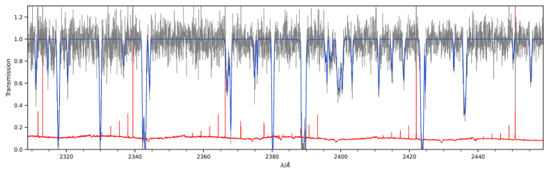
Figure 4: An example of the mock spectrum (grey) forward-modelled from one of the STIS quasar spectra (segments), with the corresponding noise vector (red). The model fitted by VPFIT is shown in the blue.

4 Inference Method

4.1 Emulating the $\left\{b,N_{{\mbox{\scriptsize\text{H\,{i}}}}{}}\right\}$ Distribution

In this work, we make use of the inference framework following Hu22, which measures the thermal state and the photoionization rate $\Gamma_{{\mbox{\scriptsize\text{H\,{i}}}}{}}$ of the low redshift IGM using its $b$-$N_{{\mbox{\scriptsize\text{H\,{i}}}}{}}$ distribution and absorber line density d$N$/d$z$. The $b$-$N_{{\mbox{\scriptsize\text{H\,{i}}}}{}}$ distribution emulator is built on density-estimation likelihood-free inference (DELFI), which turns inference into a density estimation task by learning the distribution of a dataset as a function of the labels or parameters (Papamakarios & Murray, 2016; Alsing et al., 2018; Papamakarios et al., 2018; Lueckmann et al., 2018; Alsing et al., 2019). Following Hu22, we make use of pydelfi, the publicly available python implementation of DELFI, which makes use of neural density estimation (NDE) to learn the sampling conditional probability distribution $P(\mathbf{d}\>|\>\boldsymbol{\theta})$ of the data summaries $\mathbf{d}$, as a function of labels/parameters $\boldsymbol{\theta}$, from a training set of simulated data. Here the data summaries $\mathbf{d}$ are [$\log\text{$N_{{\mbox{\scriptsize\text{H\,{i}}}}{}}${}}$, $\log b$], and our set of label parameters $\boldsymbol{\theta}$ are the IGM thermal and ionization state [$\log T_{0}$, $\gamma$, $\log\Gamma_{{\mbox{\scriptsize\text{H\,{i}}}}{}}$].

We generate training datasets by labelling the $\left\{b,N_{{\mbox{\scriptsize\text{H\,{i}}}}{}}\right\}$ pairs obtained from our mock spectra with the aforementioned labels. We then train the neural network on the summary-parameter pairs $\{[\log T_{0},\gamma,\log\Gamma_{{\mbox{\scriptsize\text{H\,{i}}}}{}}],[b,\log\text{$N_{{\mbox{\scriptsize\text{H\,{i}}}}{}}${}}]\}$. Our $b$-$N_{{\mbox{\scriptsize\text{H\,{i}}}}{}}$ distribution emulator learns the conditional probability distribution $P(b\mathbin{,}N_{{\mbox{\scriptsize\text{H\,{i}}}}{}}\,\>|\>\,T_{0},\gamma,\log\Gamma_{{\mbox{\scriptsize\text{H\,{i}}}}{}})$. These conditional $b$-$N_{{\mbox{\scriptsize\text{H\,{i}}}}{}}$ distributions are then used in our inference algorithm, where we try to find the best-fit model given the observational/mock dataset, which is described in the following section. It is worth mentioning that we train our $b$-$N_{{\mbox{\scriptsize\text{H\,{i}}}}{}}$ distribution emulator for each redshift bin separately based on the corresponding training datasets.

4.1.1 Likelihood function

In Bayesian inference, a likelihood $\mathcal{L}=P(\mathrm{data}|\mathrm{model})$ is used to describe the probability of observing the data for any given model. We adopt the likelihood formalism introduced in Hu22, which is summarized as follows,

$$\ln\mathcal{L}=\sum_{i=1}^{n}\ln(\mu_{i})-\left(\frac{\text{d}N}{\text{d}z}\right)_{\rm model}\Delta z_{\rm data},$$ (3)

where $\mu_{i}$ is the Poisson rate of an absorber occupying a cell in the $b$-$N_{\rm HI}$ plane with area $\Delta{\text{N}_{{\mbox{\scriptsize\text{H\,{i}}}}{},i}}\times\Delta b_{i}$, i.e.

$$\mu_{i}=\left(\frac{\text{d}N}{\text{d}z}\right)_{\rm model}\,P(b_{i},N_{{\mbox{\scriptsize\text{H\,{i}}}}{},i}\>|\>\boldsymbol{\theta})\,\Delta{N_{{\mbox{\scriptsize\text{H\,{i}}}}{}}}\,\Delta b\,\Delta z_{\rm data}.$$ (4)

The $P(b_{i},\text{N}_{{\mbox{\scriptsize\text{H\,{i}}}}{},i}\>|\>\boldsymbol{\theta})$ in the equation is the probability distribution function at the point $(b_{i},N_{{\mbox{\scriptsize\text{H\,{i}}}}{},i})$ for any given model parameters $\boldsymbol{\theta}$ evaluated by the DELFI $b$-$N_{{\mbox{\scriptsize\text{H\,{i}}}}{}}$ distribution emulator. The $\Delta z_{\rm data}$ is the total redshift pathlength covered by the quasar spectra from which we obtain our $\left\{b,N_{{\mbox{\scriptsize\text{H\,{i}}}}{}}\right\}$ dataset, and $\left({\text{d}N}/{\text{d}z}\right)_{\rm model}$ is the absorber density which is evaluated for any given set of parameters using a Gaussian process emulator (based on George, see Ambikasaran et al. 2016), which is also trained on our training datasets obtained from the Nyx simulation suite. More information on the likelihood function and the DELFI emulator can be found in Hu22.

5 Results

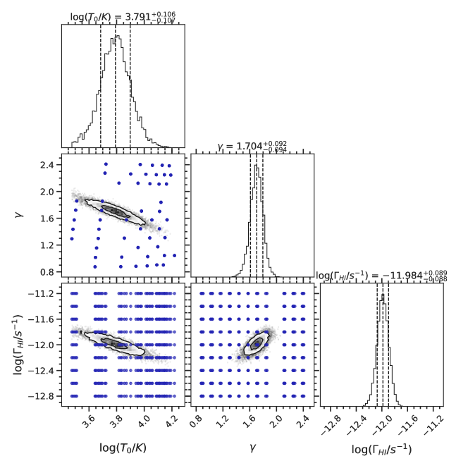
Figure 6: The MCMC posterior obtained by our inference method using our $\left\{b,N_{{\mbox{\scriptsize\text{H\,{i}}}}{}}\right\}$ dataset at $z=1.2$. Projections of the thermal grid used for generating models are shown as blue dots, while the true model is shown as red dots. The inner (outer) black contour represents the projected 2D 1(2)-sigma interval. Red lines in the marginal distributions indicate the parameters of true models, while the dashed black lines indicate the 16, 50, and 84 percentile values of the marginalized 1D posterior.

We applied the aforementioned inference method to our dataset at three redshift bins to measure the IGM thermal and ionization state at $z=$ 1.4, 1.2, and 1.0. The resulting MCMC posteriors are presented in Fig. 5, Fig. 6 and Fig. 7 respectively. Projections of the thermal grid used for generating models are shown as blue dots. The inner (outer) black contour represents the projected 2D 1(2)-sigma interval. The dashed black lines indicate the 16, 50, and 84 percentile values of the marginalized 1D posterior. For $z=1.0$ and 1.4, our preliminary results indicate that the observational data favour models with high temperature, and the MCMC posterior is truncated at the boundary of the parameter space. As described in § 3.1.2, these models with high temperatures are hard to model due to the heating mechanism used in the Nyx simulation. We thus manually rescale the temperature of some of the Nyx models and extend the parameter grid for our inference procedure as described in § 3.1. With these rescaled models, we are able to measure the thermal and ionization state of the IGM. The parameter grids that contains the rescaled models are shown in Fig. 5 and Fig. 7 for z=1.4 and z=1.0 respectively. The Nyx models used for temperature rescaling are shown as green dots, and the models with 2.5 and 3.0 times $T_{0}$ are shown as orange and red dots respectively.

We summarize the inference results (median values of the marginalized 1D posteriors for each parameter) in Table. 3.

Table 3: Summary of the inference results

$z$ bins	$\log(T_{0}/\text{K})$	$\gamma$	log ($\Gamma_{{\mbox{\scriptsize\text{H\,{i}}}}}/{\rm s}^{-1}$)
$1.3<z\leq 1.5$	${4.119}^{+0.152}_{-0.253}$	${1.341}^{+0.208}_{-0.258}$	${-11.789}^{+0.181}_{-0.147}$
$1.1<z\leq 1.3$	${3.791}^{+0.106}_{-0.107}$	${1.704}^{+0.092}_{-0.094}$	${-11.984}^{+0.089}_{-0.088}$
$0.9\leq z\leq 1.1$	${4.132}^{+0.115}_{-0.103}$	${1.357}^{+0.102}_{-0.151}$	${-12.320}^{+0.103}_{-0.115}$

• The inference results i.e., median values of the marginalized 1D posteriors for each parameter, for all three redshift bins. The errors are given by the 1-$\sigma$ error (16-84%) of the marginalized 1D posteriors.

The $\left\{b,N_{{\mbox{\scriptsize\text{H\,{i}}}}{}}\right\}$ data and the corresponding $b$-$N_{{\mbox{\scriptsize\text{H\,{i}}}}{}}$ distributions emulated by our DELFI emulator are shown in Fig. 8, and the likelihood contours corresponding to 80, 60, 40, and 20 cumulative percentiles are plotted as grey dashed lines. These plots show good agreement between the observational data and the emulated $b$-$N_{{\mbox{\scriptsize\text{H\,{i}}}}{}}$ distributions. We notice the inference result at $z=1.4$ has huge uncertainty due to the lack of observational data. However, the precision is still satisfactory, given the fact that our $\left\{b,N_{{\mbox{\scriptsize\text{H\,{i}}}}{}}\right\}$ sample at this redshift bin contains only 39 data points. Such a size is comparable with the one used in Ricotti et al. (2000), whereas the error bar is much smaller (see Fig. 12), which mainly because of our novel method using full $b$-$N_{{\mbox{\scriptsize\text{H\,{i}}}}{}}$ distribution (see Hiss et al., 2019, for the relevant discussion).

Based on the marginalized 2D posteriors, we observe that our results across all redshift bins exhibit the anticipated degeneracies between parameters. Specifically, $T_{0}$ is degenerate with both $\gamma$ and $\Gamma_{{\mbox{\scriptsize\text{H\,{i}}}}}$, as indicated in Hu22. To further assess the goodness of our inference results, we plot the marginalized 1D $b$ and $N_{{\mbox{\scriptsize\text{H\,{i}}}}}$ distributions of our sample in Fig. 9, Fig. 10, and Fig. 11 for each redshift bin, and compare them with 5000 mock datasets with the same size, sampled from the $b$-$N_{{\mbox{\scriptsize\text{H\,{i}}}}{}}$ distributions emulated based on the median values of the MCMC posteriors. The blue bars indicate the mean value of the number of lines that fall in each bin for the 5000 datasets, whereas the blue shaded regions represent the 1-$\sigma$ uncertainty calculated from the 5000 datasets. From the results, it is evident that our inference method adeptly recovers both the 2D and marginalized 1D distributions of $\left\{b,N_{{\mbox{\scriptsize\text{H\,{i}}}}{}}\right\}$, even though the limited data size, particularly at $z=1.4$, leads to noticeable fluctuations, which are underscored by the substantial 1-$\sigma$ error bar in the marginalized 1D distributions in both $b$ and $N_{{\mbox{\scriptsize\text{H\,{i}}}}}$ distributions.

As illustrated in Fig. 9, Fig. 10, and Fig. 11, our 1D $b$-parameter distributions emulated for best fit [$T_{0}$, $\gamma$, $\Gamma_{{\mbox{\scriptsize\text{H\,{i}}}}}$] are in good match with the observations, highlighting the robustness of our inference and suggesting that there is no severe discrepancy in $b$ distribution as opposed to the what is seen at $z<0.5$ (Gaikwad et al., 2017b; Viel et al., 2017). Note that this $z<0.5$ $b$-parameter discrepancy arises from studies based on COS low-$z$ Ly$\alpha$ spectra (Danforth et al., 2016), however, in reality, the spectral resolution and LSF of COS may not be very good for accurate $b$-parameter measurements, especially for small $b$ values. In contrast, old studies on higher-resolution STIS spectra, although with high uncertainty, found observed $b$-parameter in good agreement with predictions from cosmological simulations (see Fig. 3 in Davé & Tripp, 2001). This consistency implies that the $b$-parameter discrepancy found in the literature may be an artifact of the limited spectral resolution provided by COS, which will be further investigated in our future work. It also suggest that it might be beneficial to study the Ly$\alpha$ forest with the higher-resolution spectra obtained with STIS.

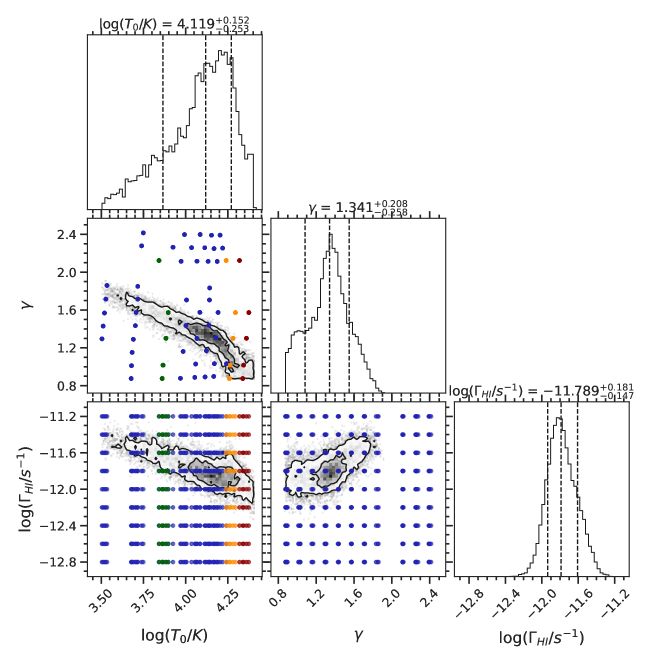
Figure 5: The MCMC posterior obtained by our inference method using our $\left\{b,N_{{\mbox{\scriptsize\text{H\,{i}}}}{}}\right\}$ dataset at $z=1.4$. Projections of the thermal grid used for generating models are shown as blue dots. The Nyx models used for temperature rescaling are shown as green dots, and the models with 2.5 and 3.0 times $T_{0}$ are shown as orange and red dots respectively. The inner (outer) black contour represents the projected 2D 1(2)-sigma interval. The dashed black lines indicate the 16, 50, and 84 percentile values of the marginalized 1D posterior.

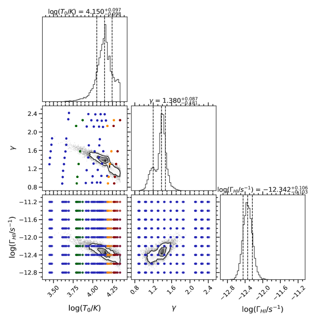
Figure 7: The MCMC posterior obtained by our inference method using our $\left\{b,N_{{\mbox{\scriptsize\text{H\,{i}}}}{}}\right\}$ dataset at $z=1.0$. Projections of the thermal grid used for generating models are shown as blue dots. The Nyx models used for temperature rescaling are shown as green dots, and the models with 2.5 and 3.0 times $T_{0}$ are shown as orange and red dots respectively. The inner (outer) black contour represents the projected 2D 1(2)-sigma interval. The dashed black lines indicate the 16, 50, and 84 percentile values of the marginalized 1D posterior.

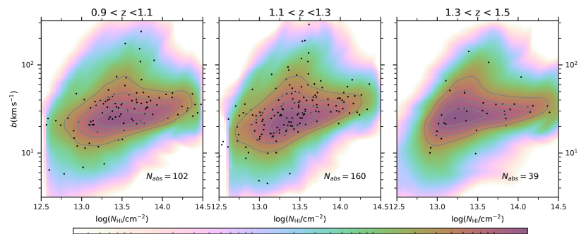
Figure 8: Joint $b$-$N_{{\mbox{\scriptsize\text{H\,{i}}}}{}}$ distributions emulated by our DELFI emulator based on the median values of the marginalized MCMC posterior at $z=$ 1.0, 1.2, and 1.4. Black dots are the $\left\{b,N_{{\mbox{\scriptsize\text{H\,{i}}}}{}}\right\}$ data. The likelihood contours corresponding to 80,60,40, and 20 cumulative percentiles CDF are plotted as gray solid lines. For illustration purposes, the values of the pdf are multiplied by 100 in the colour bar.

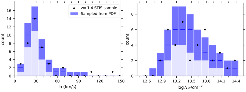
Figure 9: The marginalized 1D $b$ and $N_{{\mbox{\scriptsize\text{H\,{i}}}}}$ distributions of our are compared with 5000 mock datasets with the same size, sampled from the $b$-$N_{{\mbox{\scriptsize\text{H\,{i}}}}{}}$ distributions emulated based on the median values of the MCMC posteriors. The black dots represent our $\left\{b,N_{{\mbox{\scriptsize\text{H\,{i}}}}{}}\right\}$ data at $z=$1.4. The blue bars indicate the mean value of the number of lines that fall in each bin for the 5000 datasets, whereas the blue shaded regions represent the 1-$\sigma$ uncertainty calculated from the 5000 datasets.

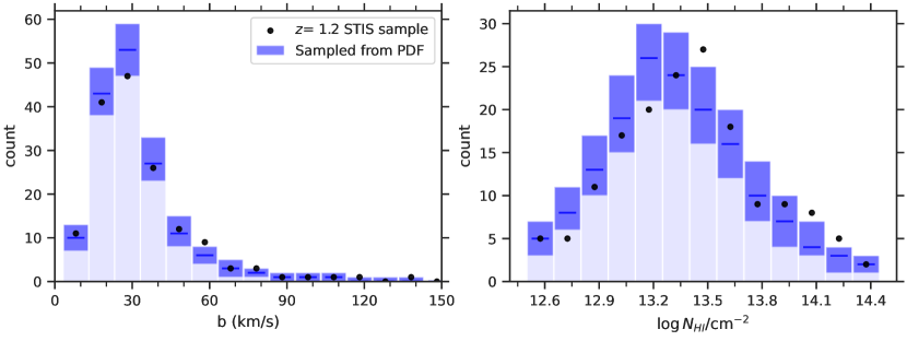
Figure 10: The marginalized 1D $b$ and $N_{{\mbox{\scriptsize\text{H\,{i}}}}}$ distributions of our are compared with 5000 mock datasets with the same size, sampled from the $b$-$N_{{\mbox{\scriptsize\text{H\,{i}}}}{}}$ distributions emulated based on the median values of the MCMC posteriors. The black dots represent our $\left\{b,N_{{\mbox{\scriptsize\text{H\,{i}}}}{}}\right\}$ data at $z=$1.2. The blue bars indicate the mean value of the number of lines that fall in each bin for the 5000 datasets, whereas the blue shaded regions represent the 1-$\sigma$ uncertainty calculated from the 5000 datasets.

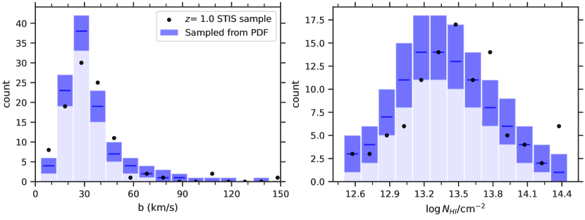
Figure 11: The marginalized 1D $b$ and $N_{{\mbox{\scriptsize\text{H\,{i}}}}}$ distributions of our are compared with 5000 mock datasets with the same size, sampled from the $b$-$N_{{\mbox{\scriptsize\text{H\,{i}}}}{}}$ distributions emulated based on the median values of the MCMC posteriors. The black dots represent our $\left\{b,N_{{\mbox{\scriptsize\text{H\,{i}}}}{}}\right\}$ data at $z=$1.0. The blue bars indicate the mean value of the number of lines that fall in each bin for the 5000 datasets, whereas the blue shaded regions represent the 1-$\sigma$ uncertainty calculated from the 5000 datasets.

5.1 Evolution of the thermal state of the IGM

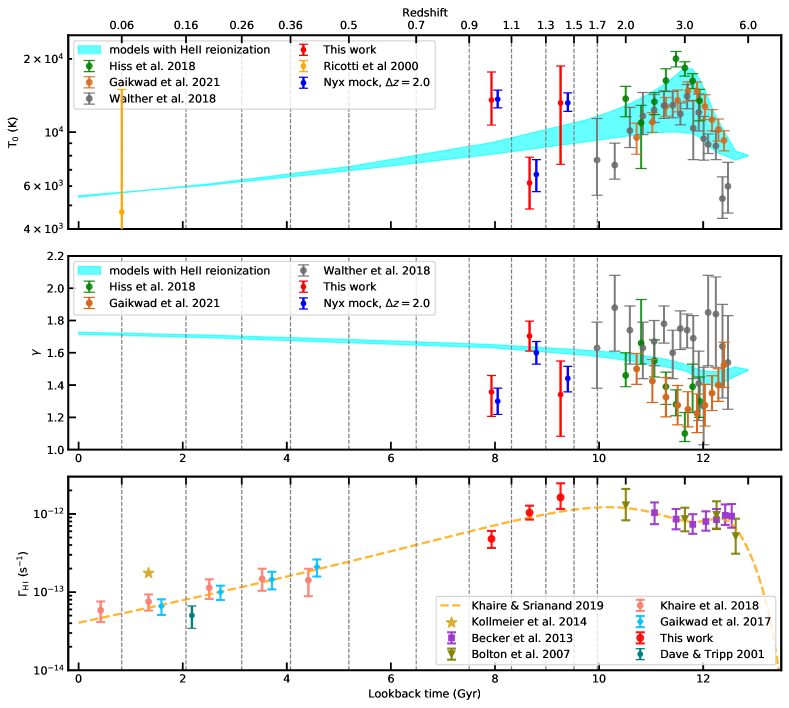
Figure 12: Evolution history of $T_{0}$ (top) and $\log\Gamma_{{\mbox{\scriptsize\text{H\,{i}}}}{}}$ (bottom) based on our inference results using the STIS data. Our results are shown as red dots, while measurements from other studies are displayed in different colours. The error bars stand for the 1-$\sigma$ error. The blue-shaded region in the top panel represents the range spanned by $T_{0}$ from hydrodynamical simulations of a large family of different HeII reionization models. The mock measurements based on Nyx simulation are shown in blue.

In Fig. 12 we summarize the $T_{0}$, $\gamma$ evolution across three redshift bins, and compare them with archival from previous studies at higher $z$ (Ricotti et al., 2000; Hiss et al., 2018; Walther et al., 2019a; Gaikwad et al., 2021). Our results and their 1-$\sigma$ uncertainties are shown as filled red data points and error bars. As a benchmark for current theoretical models, we plot the IGM thermal history spanned by all potential Helium reionization models (Oñorbe et al., 2017b, a) as the cyan-shaded region. To further assess how well do our low-$z$ results agree with previous results, in Fig. 13, we fit a power law relationship between $T_{0}$ and $z$ (blue dashed line), i.e., $\log{T_{0}}(z)=c_{1}z+c_{2}$, where $c_{1},c_{2}$ are fitting coefficients obtained from a least squares linear fit based on all previous $T_{0}$ measurements in between $1.5\leq z\leq 3.0$ (i.e., not including our measurements). Such a power law fit is a reasonable approximation in between $1.0\leq z\leq 3.0$ (see the prediction of low-$z$ $T_{0}$ in Upton Sanderbeck et al., 2016; McQuinn & Upton Sanderbeck, 2016). The power law relationship (blue dashed line in Fig. 13) suggests that our measurements at $z=1.2$ and 1.4 are consistent with previous results. However, a noticeable discrepancy in $T_{0}$ emerges at $z=1.0$, where our measurement of $T_{0}$  13500 K is significantly higher than best-fit power-law relationship predicted by previous measurements. Such a discrepancy suggests that the IGM may be far hotter than expected at $z\sim 1.0$, implying the existence of extra heating sources that are not included in our current IGM model, which becomes crucial at $z\sim 1.0$. Summarizing the $T_{0}$ measurements across all three redshift bins, two potential thermal histories for the IGM emerge: (1) The IGM might undergo a cooling phase around $z\sim 1.2$ before heating up to 13500 K at $z\sim 1.0$, which is not unfeasible given the significantly large time span of $\sim 700$ Myr between these two redshifts. (2) Alternatively, the IGM could consistently maintain a high temperature since $z\sim 1.5$. However due to the substantial error bars in $T_{0}$ in all three redshift bins, no definitive conclusion can be made until further investigation with larger datasets.

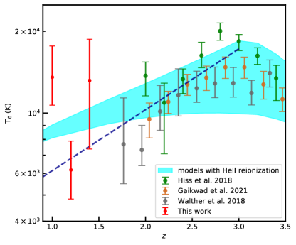
Figure 13: The evolution of $T_{0}$ in the IGM across $0.9<z<3.5$, with results from previous studies shown in comparison. The power law fit of $\log(T_{0}/\text{K})$ obtained by fitting all previous results in between $0.9<z<3.0$ are plotted as dark cyan dashed line.

To further investigate the possibe change of the IGM thermal state from $z=1.2$ to $z=1.0$, in Fig. 14, we over-plot the likelihood contours of the $b$-$N_{{\mbox{\scriptsize\text{H\,{i}}}}{}}$ distribution at $z=1.2$ on top of the $\left\{b,N_{{\mbox{\scriptsize\text{H\,{i}}}}{}}\right\}$ dataset and the corresponding $b$-$N_{{\mbox{\scriptsize\text{H\,{i}}}}{}}$ distribution at $z=1.0$. It can be seen that the $\left\{b,N_{{\mbox{\scriptsize\text{H\,{i}}}}{}}\right\}$ dataset and the corresponding $b$-$N_{{\mbox{\scriptsize\text{H\,{i}}}}{}}$ distribution at $z=1.0$ lies above the likelihood contours of the $b$-$N_{{\mbox{\scriptsize\text{H\,{i}}}}{}}$ distribution at $z=1.2$, suggesting that our observational data indeed favour a rapid change in the IGM thermal state between $1.0<z<1.2$.

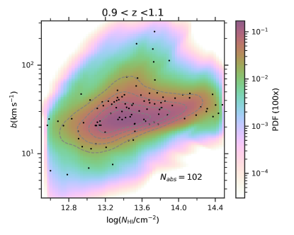
Figure 14: The likelihood contours of the $b$-$N_{{\mbox{\scriptsize\text{H\,{i}}}}{}}$ distribution at $z=1.2$ on top of the $\left\{b,N_{{\mbox{\scriptsize\text{H\,{i}}}}{}}\right\}$ dataset and the corresponding $b$-$N_{{\mbox{\scriptsize\text{H\,{i}}}}{}}$ distribution at $z=1.0$. The likelihood contours corresponding to 80,60,40, and 20 cumulative percentiles are plotted as gray dashed lines.

More discussion on this unexpected high $T_{0}$ is present in § 6.1.

As for $\gamma$, our results for $z=1.4$ and 1.2 align with this trend as outlined in McQuinn (2016), in which the value of $\gamma$ tends to decrease towards lower redshifts. However, the result at $z=1.0$ indicates a reduced $\gamma$. The cause of this discrepancy remains unclear, but it is worth noting that such a trend of $T_{0}$ and $\gamma$, i.e., high $T_{0}$, low $\gamma$, is consistent with the $T_{0}$-$\gamma$ degeneracy shown in the inference posterior (see the 2D marginalized posterior contours in $T_{0}$-$\gamma$ plane in Fig. 7). As a result, it is likely that the inference results at $z=1.0$, which yields high $T_{0}$ and low $\gamma$ are caused by inference uncertainty and degeneracy. On the other hand, it is also possible that the IGM starts to heat up at $z\sim 1.0$, leading to both increasing $T_{0}$ and decreasing $\gamma$. In this case, the inconsistencies observed in both $\gamma$ and $T_{0}$ have a common root cause.

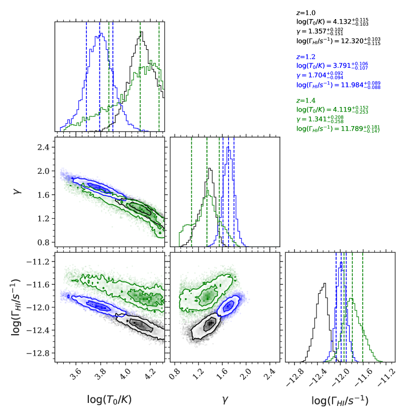
Figure 15: The MCMC posteriors obtained by our inference method for all three redshift bins. The $z=1.0$ posterior is shown in black, the $z=1.2$ posterior is shown in blue, and the $z=1.4$ posterior is shown in green.

To illustrate the evolution of the IGM thermal and ionization state, we over-plot the three MCMC posterior on top of each other in Fig. 15, where the 2D marginalized posterior for $z=1.4$ are shown in green, the one for $z=1.2$ is plotted in blue, and the one for $z=1.0$ is shown in black. From the $T_{0}$-$\gamma$ plane, we observe a clear turnover for both $T_{0}$ and $\gamma$ at $z=1.0$, suggesting a reverse evolution trend at $z\sim 1.0$. Such synchronization between the evolution of $T_{0}$ and $\gamma$ is important for us to understand the origin of the discrepancy, and relevant discussion is presented in § 6.1.

5.2 Evolution of the H i photoionization rate and the UVB

Our measurements fill in the $\Gamma_{{\mbox{\scriptsize\text{H\,{i}}}}}$ evolution history between $0.0<z<1.7$. In the bottom panel of Fig. 12 we show our $\Gamma_{{\mbox{\scriptsize\text{H\,{i}}}}}$ measurements across our three redshift bins, compared with previous studies (Davé & Tripp, 2001; Bolton, 2007; Becker & Bolton, 2013; Kollmeier et al., 2014; Gaikwad et al., 2017b; Khaire et al., 2019). Our inference results indicate that the $\Gamma_{{\mbox{\scriptsize\text{H\,{i}}}}{}}$ is in good agreement with the UVB model presented in Khaire & Srianand (2019) in all three redshift bins.

It is worth noting that for $z<3$, the UVB model of Khaire & Srianand (2019) is dominated by photons emitted by quasars alone i.e., the escape fraction on ionizing photons from galaxies is negligible at $z<3$. Our $\Gamma_{{\mbox{\scriptsize\text{H\,{i}}}}{}}$ measurements support the same conclusion that galaxies are not the main source of ionizing photons at $z<3$. The same conclusion can be drawn from the new UVB models of Puchwein et al. (2019) and Faucher-Giguère (2020) because their $\Gamma_{{\mbox{\scriptsize\text{H\,{i}}}}{}}$ values align very well with the UVB model of (Khaire & Srianand, 2019) at $z<2$. This is mainly because all three UVB models use updated quasar luminosity functions at $z<3$ (as presented in Croom et al., 2009; Ross et al., 2013; Palanque-Delabrouille et al., 2013) after Khaire & Srianand (2015) pointed out that previous UVB models (Haardt & Madau, 2012; Faucher-Giguère et al., 2009) used old quasar luminosity function that predicts factor two smaller ionizing emissivity.

The consistency of our new $\Gamma_{{\mbox{\scriptsize\text{H\,{i}}}}{}}$ measurements in the previously unexplored redshift range with recent UVB models attests to the robustness of these UVB synthesis models, especially in the aspect of hydrogen ionizing part of the UVB.

6 Discussion

6.1 The discrepancy in $T_{0}$

In this section, we delve into the observed discrepancy in IGM thermal state at $z\sim 1.0$. First of all, we notice a coherence between the high $T_{0}$ measured at $z\sim 1$ and the high $b$-values observed at $z\sim 0.1$, based on the COS Ly$\alpha$ forest dataset (Danforth et al., 2016), where the observed $b$-parameter significantly surpass the predicted value based on various simulations (Gaikwad et al., 2017b; Viel et al., 2017; Nasir et al., 2017; Bolton et al., 2022b, a). Quantitatively, Viel et al. (2017) compares the marginalized $b$ distribution with various simulations, showing that the $b$ distribution at $z\sim$ 0.1 can be best recovered by the hydrodynamic simulations (P-GADGET-3, see Springel et al., 2005) with $T_{0}\gtrsim 10000$ K, while the theoretical model dictates that the $T_{0}\sim 5000$ at $z=0.1$. The similarity of required IGM temperature at both $z=0.1$ and 1.0 suggests that the discrepancy at $z\sim 0.1$ may be related the one at $z\sim 1$, indicating a persistent trend from $z\sim 1.0$ to $0.1$. Additionally, it also suggests that the discrepancy observed at $z=0.1$ may not be attributable to the limited resolution of the COS.

The simplest explanation for these discrepancies is the thermal broadening caused by a higher-than-expected IGM temperature, which requires the existence of extra heating sources. If this is true, our understanding of IGM physics will be changed drastically, highlighting a severe need to investigate processes that are possibly responsible for it, such as dark matter annihilation (Araya & Padilla, 2014; Bolton et al., 2022a), gamma-ray sources (Puchwein et al., 2012), or feedback from galaxy formation, whose effects are not fully understood in low-$z$ (see Springel et al., 2005; Croton et al., 2006; Sijacki et al., 2007; Hopkins et al., 2008; Tillman et al., 2023b, a; Hu et al., 2023).

Another possible explanation instead of extra heating is the presence of unexpected non-thermal broadening mechanisms affecting the $b$-parameter of the Ly$\alpha$ forest, such as micro-turbulence motion in the IGM induced by jet or feedback (Gaikwad et al., 2017b; Viel et al., 2017; Nasir et al., 2017; Bolton et al., 2022b). However, these non-thermal broadening models fail to account for the unexpected trend in $\gamma$ observed in our results, where the $\gamma$ are lower than expected at $z=1.0$. To further investigate this, we plan to apply our inference method to the COS Ly$\alpha$ forest dataset at $z\leq 0.5$, which should help to break the degeneracy between $T_{0}$ and $\gamma$, thereby providing deeper insight into the $b$ discrepancy observed at $z\sim 0.1$.

6.2 Forecast based on mock observations

In this section, we make realistic forecasts for our future measurements with more abundant observational data. Given the amount of the newfound bright objects expected in upcoming surveys including Gaia DR3 (Gaia Collaboration et al., 2016, 2023). With a realistic amount of the observation from HST STIS, i.e., $\sim 50$ orbits, we expect the path length coverage for each redshift bin to be significantly extended. Here we assess the constraining power based on total pathlength $\Delta z=2$ for each redshift bin, corresponding to three times the current data size or roughly 15 spectra for each redshift bin, while assuming the characteristic SNRs of the data do not change. We pick forward-modelled mock spectra from our mock dataset at each redshift bin and generate mock observational data with total pathlength $\Delta z$=2. The Nyx model used here is the one with the thermal state that is closest to the inference results presented in § 5. The inference results obtained from these mock observations and their 1-$\sigma$ error bars are shown in Fig. 12 as blue dots. It can be seen that with $\Delta z=2$, the 1-$\sigma$ errors for $T_{0}$ become roughly $\sim 1500$ K, and the 1-$\sigma$ errors for $\gamma$ become roughly $\sim 0.08$. These results will help us to confirm whether the IGM cools down as predicted.

6.3 The effect of potential contamination

In spite of the careful masking procedure, our $\left\{b,N_{{\mbox{\scriptsize\text{H\,{i}}}}{}}\right\}$ dataset still encounters potential contaminants, including blended lines and unidentified metal lines, especially for the metal masks obtained from Milutinović et al. (2007), since their metal identification might not be complete. Here we briefly discuss the potential effects of these contaminants. It is well known that ionic metal line transitions mainly contribute to narrow absorption lines with $b\leq 10$ km/s (Schaye et al., 1999; Rudie et al., 2012b; Hiss et al., 2018). As a result, the metal line contaminants tend to bias our inference toward lower $T_{0}$. To this end, these contaminants shall not affect the main and most important result of this paper, i.e., the IGM seems to be hotter than expected at low-$z$, especially at $z=1.0$. For these blended lines, in this paper, we adopt a more conservative metal masking, where we manually filter out all suspicious lines close to the masked regions (see the masks in Appendix A). As for a more detailed quantitative analysis, we plan to identify all Ly$\alpha$ lines using the Ly$\beta$ (or higher transitions) forest (see e.g. Rudie et al., 2012b). We plan to do this in future by combining our data set with other archival and upcoming data form HST.

6.4 The effect of SNRs of the spectra

We notice that a few quasar sightlines in our sample have relatively low SNRs (see Table. 1), and it is unknown whether our results are biased by these spectra. Hence, in this section, we test the effect of these low-SNR sightlines on our inference results. To do that, we exclude three quasar spectra from our sample which have relatively lower SNR ($\leq 5$), while the remaining spectra all have SNR $>$5. We exclude TON153, PG1248+401 and PG1241+176 from the observational data and obtain a new $\left\{b,N_{{\mbox{\scriptsize\text{H\,{i}}}}{}}\right\}$ dataset, which provides 25 fewer Ly$\alpha$ lines compared with the old one and reduces the total pathlength $\Delta z$ by 0.24. We generate new mock datasets based on the nine spectra with SNR $>$ 7, and train our emulators based on the new dataset. The outcomes indicate that even after excluding low SNR spectra from our data (and correspondingly in our mock data), the results remain consistent across each redshift bin. Such a result is important for our future work, suggesting that it is possible to make use of relatively low SNR data to obtain higher total pathlength and analyse the evolution of the thermal and ionization state on finer redshift bins, such that we could pinpoint the onset of the discrepancy in $T_{0}$ (or $b$-parameter) between the observation and simulation more precisely.

7 Summary and Conclusion

In this paper, we make use of 12 archival STIS E230M quasar spectra, from which we obtain the $b$-$N_{{\mbox{\scriptsize\text{H\,{i}}}}{}}$ distribution distribution and line density d$N$/d$z$ over the redshift range $0.9<z<1.5$ in three redshift bins. We then measure the thermal and ionization state of the IGM following a machine-learning-based inference method presented in Hu22 for this redshift range for the first time. Below we summarize our resutls:

• We Voigt-profile fit the Ly$\alpha$ in all 12 quasar spectra using a fully automated VPFIT wrapper and obtain $\left\{b,N_{{\mbox{\scriptsize\text{H\,{i}}}}{}}\right\}$ for 341 lines. We use the metal identifications from the CASBaH project and combine them with the metal identification from Milutinović et al. (2007) to generate our metal masks, filtering out 40 contaminants besides Ly$\alpha$ absorption lines, and obtain a final sample of 301 Ly$\alpha$ lines across a total pathlength of $\Delta z=$2.097.

• We employ the Hu22 inference method, which simultaneously measures $[T_{0},\gamma,\Gamma_{{\mbox{\scriptsize\text{H\,{i}}}}}]$ from the $b$-$N_{{\mbox{\scriptsize\text{H\,{i}}}}{}}$ distribution and d$N$/d$z$, with the help of neural density estimators and Gaussian process emulators trained on a suite of 51 Nyx simulations each having a different IGM thermal history. It enables us to measure the IGM thermal and ionization state with high precision even with limited data.

• We obtain $[\log T_{0},\gamma]=[{4.119}^{+0.152}_{-0.253},{1.341}^{+0.208}_{-0.258}]$ at $z=1.4$ and $[\log T_{0},\gamma]=[{3.791}^{+0.106}_{-0.107},{1.704}^{+0.092}_{-0.094}]$ at $z=1.2$. These two measurements agree with the theoretical model (Fig. 12 and 13), suggesting that the thermal state of the IGM evolves as expected from $z=1.4$ to $z=1.2$.

• Nevertheless, our results yield $[\log T_{0},\gamma]$ = [${4.132}^{+0.115}_{-0.103}$, ${1.357}^{+0.102}_{-0.151}$ ] at $z=1$, suggesting an unexpectedly high IGM temperature and low $\gamma$, which is against the trend predicted by the current theoretical models of the IGM. Such high $T_{0}$ potentially suggests the existence of extra heating or unexpected non-thermal broadening at $z\sim 1.0$.

• Based on our measurements, it is possible that the IGM experiences a cooling phase until $z\sim 1.2$ from $z\sim 3$, and then it gets heated up to 13500 K at $z=1$ in approximately $700$ Myr. Alternatively, the IGM temperature might have remained consistently high since $z\sim 2$. However, due to significant uncertainties in $T_{0}$ for all three redshift bins, a definitive conclusion cannot be reached without further investigation.

• The inference results of $\gamma$ suggest that it also goes through unexpected evolution at $z\sim 1$. However, while it is likely that such a trend is caused by extra heating that causes the discrepancy in $T_{0}$, it is also possible that it is due to inference degeneracy between $T_{0}$ and $\gamma$.

• We compare our findings with previous work, which reports unanticipated high $b$-parameters compared with various simulations based on observational data at $z\sim 0.1$. These high $b$ values, if caused by thermal broadening, correspond to an IGM temperature with $T_{0}\sim 10000$K. This convergence towards a higher IGM temperature aligns with our findings and suggests that the discrepancy in $b$-parameter observed at $z\sim 0.1$ (Gaikwad et al., 2017b; Viel et al., 2017) could be related to the one we have identified in this study. It further implies that the observed discrepancy may emerge around $z\sim 1.0$ and persist down to $z\sim 0$.

• We successfully measure the $\Gamma_{{\mbox{\scriptsize\text{H\,{i}}}}}$ at three redshif bins, reporting $\Gamma_{{\mbox{\scriptsize\text{H\,{i}}}}}={-11.789}^{+0.181}_{-0.147}$, ${-11.984}^{+0.089}_{-0.088}$, and ${-12.320}^{+0.103}_{-0.115}$ at $z=1.4,1.2$ and $1.0$ respectively. These measurements align well with the predictions of recent UVB synthesis models (Khaire & Srianand, 2019; Puchwein et al., 2019; Faucher-Giguère, 2020), reinstating the fact that low-z UV background (at $z<3$) is dominated by radiation from quasars alone.

• By excluding three spectra with relatively low SNRs from our quasar sample, we confirm that our results are not sensitive to the SNR of the dataset, suggesting that it is feasible to conduct our analysis on larger quasar samples with lower SNR to make finer measurements of the IGM thermal and ionization state, so as to pinpoint the onset of the discrepancy in the IGM thermal state between the observation and simulation more precisely.

• We perform mock measurements using realistic datasets based on Nyx simulation to forecast the constraining power for our future work. The results demonstrate that with redshift pathlength $\Delta z\sim 2.0$ for each redshift bin, three times the current data size, we will be able to constrain the $T_{0}$ within $\pm$ 1500 K. This precision will help us to constrain the thermal history of the IGM in $0.9<z<1.5$, and confirm whether the IGM cools down as expected at $z\sim 1.0$.

Alongside our quasar sample, we have acquired approximately 15 additional archival STIS spectra across $0.5<z<2$, which is roughly half the size needed to draw a comprehensive picture of the low-$z$ IGM thermal evolution. After metal identification, these spectra can be incorporated into our analysis easily. We are also in the process of obtaining more observational data from the HST. Furthermore, we also planned to apply our inference methodology to simulations that utilize more sophisticated and diverse feedback mechanisms, such as those featured in EAGLE (Schaye et al., 2015) and the CAMELS suite (Villaescusa-Navarro et al., 2021). These efforts will deepen our understanding of how different feedback processes affect the low-$z$ IGM, and help investigate the causes behind the discrepancies observed between simulations and observations in the thermal state of the low-$z$ IGM.

AGN

active galactic nuclei

CMB

Cosmic Microwave Background

COS

Cosmic Origins Spectrograph

DELFI

density-estimation likelihood-free inference

DM

dark matter

DLA

damped Ly$\alpha$

GP

Gaussian process

HIRES

High Resolution Echelle Spectrometer

HST

Hubble Space Telescope

IGM

intergalactic medium

KDE

Kernel Density Estimation

KODIAQ

Keck Observatory Database of Ionized Absorbers toward QSOs

LD

least absolute deviation

LLS

Lyman limit systems

LS

least squares

LSF

line spread function

MCMC

Markov chain Monte Carlo

MW

Milky Way

NDE

neural density estimation

PCA

principal component analysis

PDF

probability density function

PKP

principal component analysis (PCA) decomposition of Kernel Density Estimation (KDE) estimates of a probability density function (PDF)

QSO

quasi-stellar objects

SNR

signal-to-noise ratio

STIS

Space Telescope Imaging Spectrograph

TDR

temperature-density relation

THERMAL

Thermal History and Evolution in Reionization Models of Absorption Lines

UV

ultraviolet

UVB

ultraviolet background

UVES

Ultraviolet and Visual Echelle Spectrograph

WHIM

warm hot intergalactic medium

CASBaH

COS Absorption Survey of Baryon Harbors

Data Availability

The simulation data and analysis code underlying this article will be shared on reasonable request to the corresponding author.

Appendix A Observational data and Metal masks

We present our observational spectra and the corresponding masks. The original spectrum is shown in grey, and the model based on VP-fitting is shown in blue. The noise vector of the original spectrum is shown in red, and the masked regions due to metal line detection are shown as green shaded regions. The Ly$\alpha$ lines used for our $\left\{b,N_{{\mbox{\scriptsize\text{H\,{i}}}}{}}\right\}$ dataset (after all filters) are labelled by red vertical lines.

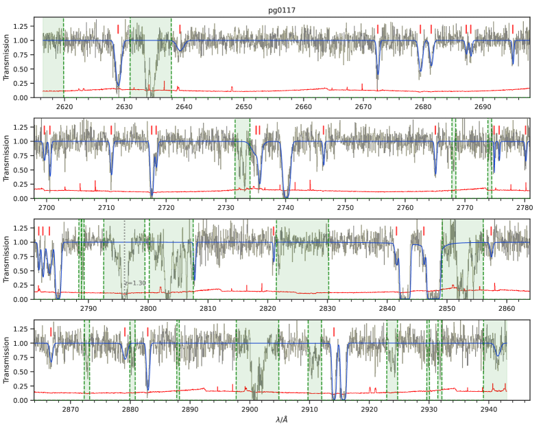
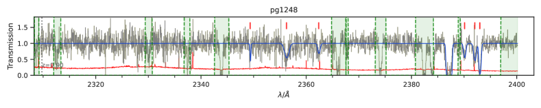
Figure 16: Illustration of the processed STIS spectrum of PG0117+213. The original spectrum is shown in gray, while a model spectrum based on line fitting (described in § 2.1) is shown in blue. The noise vector of the original spectrum is shown in red, and the masked regions are shown as a green shaded region. The Ly$\alpha$ lines used for our $\left\{b,N_{{\mbox{\scriptsize\text{H\,{i}}}}{}}\right\}$ dataset are labelled by red vertical line.

Fig. 16 continued. Spectrum of PG1248+401.

Fig. 16 continued. Spectrum of PG1522+101.

Fig. 16 continued. Spectrum of PG1634+706.

Fig. 16 continued. Spectrum of PG1718+481.

Fig. 16 continued. Spectrum for PHL1377. Fig. 16 continued. Spectrum of HE0515-4414.

Fig. 16 continued. Spectrum of LBQS1435-0134.

Fig. 16 continued. Spectrum of PG1241+176.

Fig. 16 continued. Spectrum of TON153.

Fig. 16 continued. Spectrum of PG1630+377.

References

- Acharya & Khaire (2022) Acharya A., Khaire V., 2022, MNRAS, 509, 5559
- Almgren et al. (2013) Almgren A. S., Bell J. B., Lijewski M. J., Lukić Z., Van Andel E., 2013, ApJ, 765, 39
- Alsing et al. (2018) Alsing J., Wandelt B., Feeney S., 2018, MNRAS, 477, 2874
- Alsing et al. (2019) Alsing J., Charnock T., Feeney S., Wandelt B., 2019, MNRAS, 488, 4440
- Ambikasaran et al. (2016) Ambikasaran S., Foreman-Mackey D., Greengard L., Hogg D. W., O’Neil M., 2016, IEEE Transactions on Pattern Analysis and Machine Intelligence, 38, 252
- Araya & Padilla (2014) Araya I. J., Padilla N. D., 2014, MNRAS, 445, 850
- Becker & Bolton (2013) Becker G. D., Bolton J. S., 2013, MNRAS, 436, 1023
- Becker et al. (2011) Becker G. D., Bolton J. S., Haehnelt M. G., Sargent W. L. W., 2011, MNRAS, 410, 1096
- Bolton (2007) Bolton J. S., 2007, The Observatory, 127, 262
- Bolton et al. (2014) Bolton J. S., Becker G. D., Haehnelt M. G., Viel M., 2014, MNRAS, 438, 2499
- Bolton et al. (2022a) Bolton J. S., Caputo A., Liu H., Viel M., 2022a, Phys. Rev. Lett., 129, 211102
- Bolton et al. (2022b) Bolton J. S., Gaikwad P., Haehnelt M. G., Kim T.-S., Nasir F., Puchwein E., Viel M., Wakker B. P., 2022b, MNRAS, 513, 864
- Burchett et al. (2019) Burchett J. N., et al., 2019, ApJ, 877, L20
- Carswell & Webb (2014) Carswell R. F., Webb J. K., 2014, VPFIT: Voigt profile fitting program (ascl:1408.015)
- Chen et al. (2017) Chen H.-W., Johnson S. D., Zahedy F. S., Rauch M., Mulchaey J. S., 2017, ApJ, 842, L19
- Croom et al. (2009) Croom S. M., et al., 2009, MNRAS, 399, 1755
- Croton et al. (2006) Croton D. J., et al., 2006, MNRAS, 365, 11
- Danforth et al. (2016) Danforth C. W., et al., 2016, VizieR Online Data Catalog, p. J/ApJ/817/111
- Davé & Tripp (2001) Davé R., Tripp T. M., 2001, ApJ, 553, 528
- Davé et al. (2010) Davé R., Oppenheimer B. D., Katz N., Kollmeier J. A., Weinberg D. H., 2010, MNRAS, 408, 2051
- Fan et al. (2006) Fan X., et al., 2006, AJ, 132, 117
- Faucher-Giguère (2020) Faucher-Giguère C.-A., 2020, MNRAS, 493, 1614
- Faucher-Giguère et al. (2008) Faucher-Giguère C.-A., Lidz A., Hernquist L., Zaldarriaga M., 2008, ApJ, 688, 85
- Faucher-Giguère et al. (2009) Faucher-Giguère C.-A., Lidz A., Zaldarriaga M., Hernquist L., 2009, ApJ, 703, 1416
- Finkelstein et al. (2019) Finkelstein S. L., et al., 2019, ApJ, 879, 36
- Fumagalli et al. (2017) Fumagalli M., Haardt F., Theuns T., Morris S. L., Cantalupo S., Madau P., Fossati M., 2017, MNRAS, 467, 4802
- Gaia Collaboration et al. (2016) Gaia Collaboration et al., 2016, A&A, 595, A1
- Gaia Collaboration et al. (2023) Gaia Collaboration et al., 2023, A&A, 674, A1
- Gaikwad et al. (2017a) Gaikwad P., Khaire V., Choudhury T. R., Srianand R., 2017a, MNRAS, 466, 838
- Gaikwad et al. (2017b) Gaikwad P., Srianand R., Choudhury T. R., Khaire V., 2017b, MNRAS, 467, 3172
- Gaikwad et al. (2018) Gaikwad P., Choudhury T. R., Srianand R., Khaire V., 2018, MNRAS, 474, 2233
- Gaikwad et al. (2021) Gaikwad P., Srianand R., Haehnelt M. G., Choudhury T. R., 2021, MNRAS, 506, 4389
- Haardt & Madau (2012) Haardt F., Madau P., 2012, ApJ, 746, 125
- Haislmaier et al. (2021) Haislmaier K. J., Tripp T. M., Katz N., Prochaska J. X., Burchett J. N., O’Meara J. M., Werk J. K., 2021, MNRAS, 502, 4993
- Hiss et al. (2018) Hiss H., Walther M., Hennawi J. F., Oñ orbe J., O’Meara J. M., Rorai A., Lukić Z., 2018, ApJ, 865, 42
- Hiss et al. (2019) Hiss H., Walther M., Oñorbe J., Hennawi J. F., 2019, ApJ, 876, 71
- Hopkins et al. (2008) Hopkins P. F., Hernquist L., Cox T. J., Kereš D., 2008, ApJS, 175, 356
- Hu et al. (2022) Hu T., et al., 2022, MNRAS, 515, 2188
- Hu et al. (2023) Hu T., Khaire V., Hennawi J. F., Onorbe J., Walther M., Lukic Z., Davies F., 2023, arXiv e-prints, p. arXiv:2308.14738
- Hui & Gnedin (1997) Hui L., Gnedin N. Y., 1997, MNRAS, 292, 27
- Hussain et al. (2017) Hussain T., Khaire V., Srianand R., Muzahid S., Pathak A., 2017, MNRAS, 466, 3133
- Khaire (2017) Khaire V., 2017, MNRAS, 471, 255
- Khaire & Srianand (2015) Khaire V., Srianand R., 2015, MNRAS, 451, L30
- Khaire & Srianand (2019) Khaire V., Srianand R., 2019, MNRAS, 484, 4174
- Khaire et al. (2016) Khaire V., Srianand R., Choudhury T. R., Gaikwad P., 2016, MNRAS, 457, 4051
- Khaire et al. (2019) Khaire V., et al., 2019, MNRAS, 486, 769
- Khaire et al. (2023a) Khaire V., Hu T., Hennawi J. F., Walther M., Davies F., 2023a, arXiv e-prints, p. arXiv:2306.05466
- Khaire et al. (2023b) Khaire V., Hu T., Hennawi J. F., Burchett J. N., Walther M., Davies F., 2023b, arXiv e-prints, p. arXiv:2311.08470
- Kimble et al. (1998) Kimble R. A., et al., 1998, in Bely P. Y., Breckinridge J. B., eds, Society of Photo-Optical Instrumentation Engineers (SPIE) Conference Series Vol. 3356, Space Telescopes and Instruments V. pp 188–202, doi:10.1117/12.324433
- Kollmeier et al. (2014) Kollmeier J. A., et al., 2014, ApJ, 789, L32
- Lehner et al. (2013) Lehner N., et al., 2013, The Astrophysical Journal, 770, 138
- Lueckmann et al. (2018) Lueckmann J.-M., Bassetto G., Karaletsos T., Macke J. H., 2018, arXiv preprint arXiv:1805.09294
- Lukić et al. (2015) Lukić Z., Stark C. W., Nugent P., White M., Meiksin A. A., Almgren A., 2015, MNRAS, 446, 3697
- Madau et al. (1998) Madau P., Pozzetti L., Dickinson M., 1998, ApJ, 498, 106
- McGreer et al. (2015) McGreer I. D., Mesinger A., D’Odorico V., 2015, MNRAS, 447, 499
- McQuinn (2016) McQuinn M., 2016, ARA&A, 54, 313
- McQuinn & Upton Sanderbeck (2016) McQuinn M., Upton Sanderbeck P. R., 2016, MNRAS, 456, 47
- McQuinn et al. (2009) McQuinn M., Lidz A., Zaldarriaga M., Hernquist L., Hopkins P. F., Dutta S., Faucher-Giguère C.-A., 2009, Apj, 694, 842
- Medallon & Welty (2023) Medallon S., Welty D., 2023, in , Vol. 22, STIS Instrument Handbook for Cycle 31 v. 22. p. 22
- Milutinović et al. (2007) Milutinović N., et al., 2007, MNRAS, 382, 1094
- Nasir et al. (2017) Nasir F., Bolton J. S., Viel M., Kim T.-S., Haehnelt M. G., Puchwein E., Sijacki D., 2017, MNRAS, 471, 1056
- Oñorbe et al. (2017a) Oñorbe J., Hennawi J. F., Lukić Z., 2017a, The Astrophysical Journal, 837, 106
- Oñorbe et al. (2017b) Oñorbe J., Hennawi J. F., Lukić Z., Walther M., 2017b, The Astrophysical Journal, 847, 63
- Palanque-Delabrouille et al. (2013) Palanque-Delabrouille N., et al., 2013, A&A, 551, A29
- Papamakarios & Murray (2016) Papamakarios G., Murray I., 2016, in Advances in Neural Information Processing Systems. pp 1028–1036
- Papamakarios et al. (2018) Papamakarios G., Sterratt D. C., Murray I., 2018, arXiv preprint arXiv:1805.07226
- Planck Collaboration et al. (2014) Planck Collaboration et al., 2014, A&A, 571, A16
- Prochaska et al. (2019) Prochaska J. X., et al., 2019, ApJS, 243, 24
- Puchwein et al. (2012) Puchwein E., Pfrommer C., Springel V., Broderick A. E., Chang P., 2012, MNRAS, 423, 149
- Puchwein et al. (2019) Puchwein E., Haardt F., Haehnelt M. G., Madau P., 2019, MNRAS, 485, 47
- Rahmati et al. (2013) Rahmati A., Pawlik A. H., Raičević M., Schaye J., 2013, MNRAS, 430, 2427
- Ricotti et al. (2000) Ricotti M., Gnedin N. Y., Shull J. M., 2000, ApJ, 534, 41
- Robertson et al. (2015) Robertson B. E., Ellis R. S., Furlanetto S. R., Dunlop J. S., 2015, ApJL, 802, L19
- Rorai et al. (2017) Rorai A., et al., 2017, Science, 356, 418
- Ross et al. (2013) Ross N. P., et al., 2013, ApJ, 773, 14
- Rudie et al. (2012a) Rudie G. C., Steidel C. C., Pettini M., 2012a, ApJ, 757, L30
- Rudie et al. (2012b) Rudie G. C., Steidel C. C., Pettini M., 2012b, ApJ, 757, L30
- Schaye et al. (1999) Schaye J., Theuns T., Leonard A., Efstathiou G., 1999, MNRAS, 310, 57
- Schaye et al. (2000) Schaye J., Theuns T., Rauch M., Efstathiou G., Sargent W. L. W., 2000, MNRAS, 318, 817
- Schaye et al. (2015) Schaye J., et al., 2015, MNRAS, 446, 521
- Shull et al. (2015) Shull J. M., Moloney J., Danforth C. W., Tilton E. M., 2015, ApJ, 811, 3
- Sijacki et al. (2007) Sijacki D., Springel V., Di Matteo T., Hernquist L., 2007, MNRAS, 380, 877
- Springel et al. (2005) Springel V., et al., 2005, Nature, 435, 629
- Tepper-García (2006) Tepper-García T., 2006, MNRAS, 369, 2025
- Tillman et al. (2023a) Tillman M. T., et al., 2023a, arXiv e-prints, p. arXiv:2307.06360
- Tillman et al. (2023b) Tillman M. T., Burkhart B., Tonnesen S., Bird S., Bryan G. L., Anglés-Alcázar D., Davé R., Genel S., 2023b, ApJ, 945, L17
- Tripp (2014) Tripp T., 2014, The COS Absorption Survey of Baryon Harbors (CASBaH): Probing the Circumgalactic Media of Galaxies from z = 0 to z = 1.5, HST Proposal ID 13846. Cycle 22
- Tripp et al. (2001) Tripp T. M., Giroux M. L., Stocke J. T., Tumlinson J., Oegerle W. R., 2001, ApJ, 563, 724
- Upton Sanderbeck et al. (2016) Upton Sanderbeck P. R., D’Aloisio A., McQuinn M. J., 2016, MNRAS, 460, 1885
- Viel et al. (2017) Viel M., Haehnelt M. G., Bolton J. S., Kim T.-S., Puchwein E., Nasir F., Wakker B. P., 2017, MNRAS, 467, L86
- Villaescusa-Navarro et al. (2021) Villaescusa-Navarro F., et al., 2021, ApJ, 915, 71
- Walther et al. (2017) Walther M., Hennawi J. F., Hiss H., Oñorbe J., Lee K.-G., Rorai A., O’Meara J., 2017, The Astrophysical Journal, 852, 22
- Walther et al. (2019a) Walther M., Oñorbe J., Hennawi J. F., Lukić Z., 2019a, ApJ, 872, 13
- Walther et al. (2019b) Walther M., Oñorbe J., Hennawi J. F., Lukić Z., 2019b, ApJ, 872, 13
- Woodgate et al. (1998) Woodgate B. E., et al., 1998, PASP, 110, 1183
- Worseck et al. (2011) Worseck G., et al., 2011, ApJl, 733, L24
- Wotta et al. (2019) Wotta C. B., Lehner N., Howk J. C., O’Meara J. M., Oppenheimer B. D., Cooksey K. L., 2019, The Astrophysical Journal, 872, 81