Are ensembles getting better all the time?

Abstract

Ensemble methods combine the predictions of several base models. We study whether or not including more models in an ensemble always improve its average performance. Such a question depends on the kind of ensemble considered, as well as the predictive metric chosen. We focus on situations where all members of the ensemble are a priori expected to perform as well, which is the case of several popular methods like random forests or deep ensembles. In this setting, we essentially show that ensembles are getting better all the time if, and only if, the considered loss function is convex. More precisely, in that case, the average loss of the ensemble is a decreasing function of the number of models. When the loss function is nonconvex, we show a series of results that can be summarised by the insight that ensembles of good models keep getting better, and ensembles of bad models keep getting worse. To this end, we prove a new result on the monotonicity of tail probabilities that may be of independent interest. We illustrate our results on a simple machine learning problem (diagnosing melanomas using neural nets).

Keywords: Ensemble methods, deep ensembles, random forests, large deviations, wisdom of crowds

1 Introduction

The idea that groups are collectively wiser than individuals can be traced back to various branches of science, ranging from political science to philosophy, economics, or sociology. It is referred to in various, sometimes colorful, ways: some, like Dekel and Shamir (2009), praise the “vox populi,” following Galton’s (1907) seminal paper; the phrase “wisdom of crowds,” used for instance by Prelec et al. (2017) or Simoiu et al. (2019), was immensely popularised by Surowiecki’s (2005) bestselling book; political scientists like Althaus (2003) often debate the virtues of the “miracle of aggregation” as a theoretical argument in favor of democracy; many scientists made the popular phrase “two heads are better than one” their own (e.g., Koriat, 2012; Chu-Carroll et al., 2003).

In statistics, forecasting, and machine learning, this idea is embodied by ensemble methods. Broadly speaking, ensembles combine the outputs of several base predictive models in a single decision, often by averaging (for regression) or by majority voting (for classification). They have been used in very different contexts, as illustrated for instance in Kuncheva’s (2014) monograph on the topic. Early applications were mostly related to forecasting (Bates and Granger, 1969; Clemen, 1989) and decision theory (Stone, 1961; Genest and Zidek, 1986). In the 1990s, a significant amount of new ensembling techniques were developed by the burgeoning machine learning community, including notably boosting (Freund and Schapire, 1997), Breiman’s bagging (1996) or random forests (2001), Ho’s (1998) random subspace method, neural network ensembles (Hansen and Salamon, 1990; Krogh and Vedelsby, 1994), and Bayesian model averaging (Hoeting et al., 1999). The success of ensembles has continued ever since: ensembles are now routinely used for probabilistic weather forecasting (Gneiting and Raftery, 2005), random forests and boosting remain the most efficient machine learning methods for tabular data (Grinsztajn et al., 2022), ensembles based on random projections are still actively researched (Cannings and Samworth, 2017), and ensembles of neural networks have been instrumental within the deep learning revolution, notably through dropout (Srivastava et al., 2014; Baldi and Sadowski, 2014; Hron et al., 2018) and deep ensembles (Lakshminarayanan et al., 2017) and their variants (see, e.g., Sun et al., 2022; Laurent et al., 2023, and references therein).

The empirical successes of ensembles seems to indicate that the more models are being aggregated, the better the ensemble is. The theoretical question we address in this paper is what we call the monotonicity question: Is it always true that an ensemble of $K+1$ models performs better than an ensemble of $K$ models? A positive answer to this question has practical consequences: given an ensemble with $K$ base models, performances will improve when using one (or ten) more.

The main heuristic justification of ensembles is that groups are collectively wiser than individuals, because aggregated decisions have a smaller variance than individual ones. Condorcet (1785) proposed a first formalisation of this insight. Indeed, his goal was to prove that, within a trial, the larger the number of jurors, the better. In modern machine learning jargon, he showed that ensembles containing an odd number of Bernoulli-distributed predictors are monotonically improving, with respect to the classification error (see Shteingart et al. 2020, for a modern proof). Surprisingly, he also noticed that monotonicity is broken if the ensemble is allowed to contain an even number of predictors.

While an important amount of work has been devoted to the theoretical study of ensembles (see, e.g., Germain et al., 2015; Scornet et al., 2015; Larsen, 2023), the monotonicity question has been quite overlooked, especially theoretically. Lam and Suen (1997) and Dougherty and Edward (2009) revisited Condorcet’s theorem, and studied the issues that make the presence of an even number of models problematic. Several generalisations of this theorem were also derived, in particular with weaker dependence assumptions (see, e.g., Ladha, 1993). Probst and Boulesteix (2018), in the context of random forests, performed a very thorough theoretical and empirical study of the monotonicity question. Their empirical conclusions were that, for some performance metrics (the cross-entropy or the Brier score for classification and the mean squared error for regression), ensembles are getting better all the time, but that is not necessarily the case for the classification error. Moreover, they provided theoretical support for some of these phenomena. Their paper was a key inspiration for this work, and our main contribution is to provide a unified view of their insights by essentially showing that ensembles are getting better all the time if, only if, the considered loss function is convex. Indeed, the cross-entropy, the Brier score, and the mean squared error are all convex losses (and always lead to monotonic improvements), whereas the classification error is not (and may lead to non-monotonicity).

The relationship between the usefulness of ensembling and convexity was perhaps first highlighted by Stone (1961) in the context of decision theory. It was further discussed by several papers in the 1990s (McNees, 1992; Perrone, 1993; Breiman, 1996; George, 1999). An interesting historical perspective on the question was provided by Manski (2010, Section 6). However, the relationship between the monotonicity question and convexity appears to have been overlooked.

Monotonicity beyond ensembles

Before we illustrate empirically the in and outs of our main question, it is worth mentioning some related work on monotonicity in statistics and machine learning. A first intriguing phenomenon is the fact that the coverage probability of a confidence interval for the true parameter of a Bernoulli random variable is non-monotonic (see, e.g., Brown et al. 2001, Figure 1). In plain words, and perhaps counter-intuitively, increasing the number of observations does not guarantee that the probability for the confidence interval to contain the true parameter increases! Another related question is the one of the monotonicity of learning: will a machine learning algorithm perform better when adding one new sample to the training set? This problem is mentioned for instance by Rasmussen and Williams (2006, Exercise 2.4), and was recently cast as an open problem by Viering et al. (2019) at the 32nd Conference on Learning Theory (COLT). Progress on that front was recently reviewed by Viering and Loog (2023).

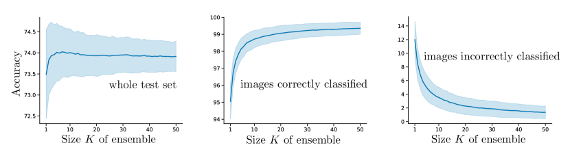
Figure 1: Evolution of the accuracy of a dropout ensemble on the dermatology data set as the number of models grows (mean and standard deviation over $500$ repetitions). (Left) The accuracy averaged over the whole test set has no clear monotonic pattern. (Middle) The accuracy averaged over images for which the asymptotic prediction $\overline{y}_{\infty}$ is correct is getting better. (Right) The accuracy averaged over images for which the asymptotic prediction $\overline{y}_{\infty}$ in incorrect is getting worse. The behaviours of these middle and right panels are explained by our theory. Notice that the three $y$-axes have different scales.

1.1 A motivating example: neural nets for medical diagnosis

In this section, we consider the following practical problem: we want to predict whether a dermatoscopic image corresponds to a benign keratosis-like lesion or a melanoma. We use the DermaMNIST (Yang et al., 2023) data set, based on the HAM10000 collection (Tschandl et al., 2018), and retain only the classes “benign keratosis” and “melanoma” (more details on the data set are available in Section LABEL:sec:experiments). Using a training set and a validation set, we train a convolutional neural network with dropout to discriminate these two classes. We then use a Monte Carlo dropout ensemble to classify the test set (Gal and Ghahramani, 2016; Hron et al., 2018), and look at the evolution of the accuracy (Figure 1) and the cross-entropy (Figure 2) as the ensemble grows. There is a crisp difference between the behaviours of the two losses. The overall accuracy has no clear monotonic pattern, but if we split the test set into two subsets depending on whether the asymptotic prediction is right or wrong, we notice that the accuracy is decreasing for right predictions and increasing for wrong ones! On the other hand, the cross entropy appears clearly decreasing, regardless of the quality of the prediction. Our goal is to provide clear theoretical explanations for these phenomena.

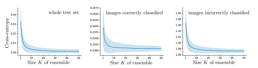
Figure 2: Evolution of the cross-entropy (or negative log-likelihood) of a dropout ensemble on the dermatology data set as the number of models grows (mean and standard deviation over 500 repetitions). (Left) Cross-entropy averaged over the whole test set. (Middle) Cross-entropy averaged over images for which the asymptotic prediction $\overline{y}_{\infty}$ is correct. (Right) Cross-entropy averaged over images for which the asymptotic prediction $\overline{y}_{\infty}$ in incorrect. As predicted by our theory, all curves are decreasing. Notice that the three $y$-axes have different scales.

1.2 Summary and organisation of the paper

In this work, we focus on the simplest instance of ensembles, that involve unweighted averaging of predictions that are “not too dependent”. While simple, this setting remains the usual formalization of most “wisdom of crowds” studies, and the basis of state-of-the-art machine learning methods like random forests and deep ensembles. In this context we show that whether or not an ensemble is monotonically improving is deeply connected to the local geometry of the chosen loss function, more specifically to its convexity and its smoothness. Informally, our results may be summarised by the sentence ensembles are getting better all the time if, and only if, the considered loss function is convex. More precisely our contributions are as follows.

• For convex loss functions and exchangeable predictions, we show that the expected loss is a non-increasing function of the number of ensembles members (Theorem 2), generalising several results previously obtained for specific losses (Noh et al., 2017; Probst and Boulesteix, 2018). This result can be strengthened for strictly convex losses (Theorem 4).

• For nonconvex loss functions and independent and identically distributed (i.i.d.) predictions, we show that, asymptotically, good ensembles keep getting better, and bad ensembles keep getting worse in the following sense:

  • when the loss if sufficiently smooth, ensembles keep eventually getting better when the loss function is locally convex at their asymptotic predictions, whereas they keep getting worse if the loss is locally concave there (Theorem 5);

  • for the classification error, ensembles keep eventually getting better when their asymptotic prediction corresponds to the true label, and keep getting worse if it corresponds to a wrong label (Theorem 8). This result comes with not-so-mild regularity conditions that we relate to classical counterexamples à la Condorcet.

• To prove our result for nonsmooth losses, we prove a new theorem on the monotonicity of tail probabilities that may be of independent interest (Theorem 7). This result is based on “strong” large deviations theorems (Bahadur and Ranga Rao, 1960; Petrov, 1965; Joutard, 2017).

2 Background, notations, and examples

We first present how to deal with a single prediction, and then why we may deal with several predictions, and how me may aggregate them.

2.1 A general predictive framework

We consider a predictive task where several kinds of methods can output predictions $\hat{y}$, living in a convex set $C$. We require the prediction set to be convex because we want that averaged predictions remain inside $C$ (this is barely a restriction, since when the prediction set is nonconvex we can simply replace it by its convex hull). The quality of these predictions can be evaluated using a loss function $L:C\rightarrow\mathbb{R}$. This broad setting contains several important cases, and we present below a few important examples. In most of these examples, $\hat{y}$ will be of the form $f(x)$, where $f$ is a predictor and $x$ a given data point. This means that $L(\hat{y})$ is the loss of an individual prediction, rather than the loss averaged over a dataset.

Supervised learning and forecasting are the main examples we are interested in. Consider a given data point $x\in\mathcal{X}$, with true label/response $y\in\mathcal{Y}$. The prediction will typically be $\hat{y}=f(x)$ where $f$ can be for instance a neural network, a random forest, or even a human expert opinion (e.g., a doctor diagnosing a patient based on their records $x$). In this setting, loss functions have the familiar form $L(\hat{y})=\ell(\hat{y},y)$ where $\ell:C\times\mathcal{Y}\rightarrow\mathbb{R}$ measures the mismatch between the true label and its prediction (see, e.g., Shalev-Shwartz and Ben-David 2014). As an example, for neural net classification with $n_{\text{cl}}$ classes, the prediction set $C$ will either be $\mathbb{R}^{n_{\text{cl}}}$ (in the absence of a final softmax layer, in this case $\hat{y}$ denotes the logits) or the ${n_{\text{cl}}}$-simplex ($\hat{y}$ will then be the output of the softmax layer). In both cases, $\ell$ will typically be the cross-entropy, defined in the case where $\hat{y}$ is the softmax output, as

$$L(\hat{y})=\ell(\hat{y},y)=\sum_{j=1}^{n_{\text{cl}}}-y_{j}\log\hat{y}_{j}\,,$$ (1)

where the true label is represented by a one-hot encoding $y=(y_{1},\ldots,y_{n_{\text{Cl}}})\in\{0,1\}^{n_{\text{Cl}}}$. Another common choice of loss function in that case is the classification error

$$L(\hat{y})=\ell(\hat{y},y)=\left\{\begin{matrix}1\;\text{ if }\;\text{argmax}(\hat{y})\neq\text{argmax}(y)\\ 0\;\text{ if }\;\text{argmax}(\hat{y})=\text{argmax}(y)\,.\end{matrix}\right.$$ (2)

If the response set is continuous (e.g., if $\mathcal{Y}=\mathbb{R}$ as in a standard regression problem), the prediction set can be simply $\mathbb{R}$ if we are simply interested in predicting a point estimate of the response, and $\ell$ can be the squared error: $L(\hat{y})=\ell(\hat{y},y)=(\hat{y}-y)^{2}$. In we are interested in the full conditional distribution of the response, $C$ can be defined as the set of probability densities over $\mathbb{R}$. The loss $\ell$ can then be any scoring rule like the negative log-likelihood $-\log\hat{y}(y|x)$ or the continuous ranked probability score, see, e.g., Gneiting and Raftery 2007. Other supervised examples with more exotic prediction spaces and loss functions include include image segmentation or ordinal regression.

Density estimation is generally unsupervised, and not directly a predictive problem. Is is nevertheless a particular case of our framework. Here, $\hat{y}$ will be a probability density over the data space $\mathcal{X}$, for instance modelled by a mixture model or a deep generative model, which means that $C$ will be the set of all densities over $\mathcal{X}$. For a given $x\in\mathcal{X}$, a popular loss function is then the negative log-likelihood $L(\hat{y})=-\log\hat{y}(x)$. Similarly to the probabilistic regression example outlined above, any scoring rule can also be chosen (e.g., score matching and its variants, commonly used for density estimation). More exotic losses include using statistical divergences between the distribution $\hat{y}$ and the empirical distribution of a test or validation set. While ensembling is less common for density estimation than forecasting and supervised learning, it has been successfully used in several contexts. For instance, Riesselman et al. (2018) used ensembles of deep generative models to model biological sequences and Russell et al. (2015) and Casa et al. (2021) have used ensembles of Gaussian mixtures for density estimation and clustering.

Statistical estimation involves an unknown parameter $\theta^{\star}\in\Theta$. In this case, $C=\Theta$ and $\hat{y}$ can be any estimator of $\theta$. A possible loss function in this example is given by $L(\hat{y})=d(\hat{y},\theta^{\star})$, where $d$ is a distance over $\Theta$. Here again, the use of ensembles is less common than for supervised learning. Nonetheless, bagging and its variants have been thoroughly studied for statistical estimation (see, e.g., Bühlmann and Yu 2002; Friedman and Hall 2007; Bach 2008).

Why is $L$ only a function of $\hat{y}$?

In many of these examples, the loss function depends on other quantities than the predictions (the features, the true label…), yet we just denote it by $L(\hat{y})$. Our analysis aims at studying the impact of the predictions on the loss, therefore we keep all these other quantities fixed, and vary only the predictions. This is why we only model our loss function $L$ as a function of the predictions $\hat{y}$. In particular, this means that our results typically concern the loss evaluated for a single given data point and a single ground truth label. Of course, we are also often interested in evaluating the loss not only on individual data points, but on batches or entire data sets. Our results on individual data points can then be extended by averaging them, as we discuss further in Section 2.2.3.

2.2 Several predictions, and how to average them

From now on, we consider that we are given $K\in\mathbb{N}^{\star}$ different predictions $\hat{y}_{1},\ldots,\hat{y}_{K}\in C$ that we wish to aggregate.

2.2.1 Where do our predictions $\hat{y}_{1},\ldots,\hat{y}_{K}$ come from?

A fundamental example to keep in mind is the situation where the predictions come from slight variations from the same model. In Breiman’s (1996) bagging, each $\hat{y}_{k}$ comes from using the same algorithm on a different bootstraped version of the original data. This is also the cornerstone of random forests, for which each $\hat{y}_{k}$ is the output of a single (random) decision tree (Breiman, 2001). Each tree has a different structure coming from the randomness of the tree construction procedure, leading to distinct, random $\hat{y}_{k}$s. Another important example, pioneered by Hansen and Salamon (1990) and popularised by Lakshminarayanan et al. (2017), uses as $\hat{y}_{k}$s the outputs of neural networks trained with different weights initialisations. Another popular way of creating ensembles of deep nets is via dropout (Srivastava et al., 2014; Baldi and Sadowski, 2014): each $\hat{y}_{k}$ is obtained by sampling a different dropout mask and applying it to the same backbone network. Gal and Ghahramani (2016) call such a technique Monte Carlo dropout.

In all the examples presented in the previous paragraph, the $\hat{y}_{1},\ldots,\hat{y}_{K}$ are i.i.d. random variables. Assumptions of this sort will be required for our proofs. Indeed, with the exception of Lemma 1, we will always require our predictions to be random variables with some (weak) dependence structure.

We want to emphasise that our framework also encompasses situations where we are given a few predictions that are fully deterministic, for instance, the forecasts of several different physical models. One way to see them as random predictions and to make them amenable to our theory is to assume that the ordering of the $\hat{y}_{1},\ldots,\hat{y}_{K}$ does not matter, or equivalently that we have no knowledge of how these models fare against each other. This can be formalised by assuming that we do not observe $\hat{y}_{1},\ldots,\hat{y}_{K}$ but $\hat{y}_{\sigma(1)},\ldots,\hat{y}_{\sigma(K)}$, where $\sigma$ is a uniformly sampled permutation of $\{1,\ldots,K\}$. Because $\sigma$ is random, $\hat{y}_{\sigma(1)},\ldots,\hat{y}_{\sigma(K)}$ is also random. While not i.i.d. in general, this randomly reordered ensemble satisfies another weaker condition called exchangeability. A sequence of random variables is exchangeable when any of its reorderings has the same distribution, we will give a formal definition in Eq. (13).

2.2.2 How to aggregate predictions?

Perhaps the simplest idea to aggregate predictions then to take their (unweighted) mean, namely to consider the prediction

$$\overline{y}_{K}=\frac{1}{K}\sum_{k=1}^{K}\hat{y}_{k}\,.$$ (3)

Note that we are allowed to consider such an aggregation since $C$ is convex, which implies that the ensemble prediction $\hat{y}$ indeed belongs to $C$. This simple aggregation scheme is used by many ensembles, for instance bagging (and in particular random forests), deep ensembles, or Monte Carlo dropout. Many other aggregation schemes have been proposed (see, e.g., Kuncheva 2014, Chapters 4 and 5), but our analysis is fundamentally tied to the simple averaging technique, so we will not discuss them further. A convenient property of $\overline{y}_{K}$ is that its asymptotic behavior is quite intuitive. Indeed, when $\hat{y}_{1},\ldots,\hat{y}_{K}$ are i.i.d. with mean $\overline{y}_{\infty}=\mathbb{E}\left[\hat{y}_{1}\right]=\cdots=\mathbb{E}\left[\hat{y}_{K}\right]$, then the law of large numbers implies that $\overline{y}_{K}\longrightarrow\overline{y}_{\infty}$ when $K\rightarrow+\infty$. We will refer to $\overline{y}_{\infty}$ as the asymptotic prediction of the ensemble.

Several other aggregation schemes can be, in some settings, equivalent to the simple average. For instance, the geometric mean can be written as a regular mean in log scale, since $\sqrt[K]{\hat{y}_{1}\cdots\hat{y}_{K}}=\exp\left(\frac{1}{K}\sum_{k=1}^{K}\log\hat{y}_{k}\right)$. The popular method of majority voting can also be seen as a form of standard average. Indeed, consider for instance a binary classification problem for which several votes $\hat{y}_{1},\ldots,\hat{y}_{K}\in\{0,1\}$ are cast for a true class $y\in\{0,1\}$. The prediction space $\{0,1\}$ is nonconvex, but we may choose to see the votes as elements of its convex hull $C=[0,1]$. A natural choice of loss function is then the classification error $L(\hat{y})$, defined by Eq. (22). The most natural way of combining these votes is to use majority voting, considering as final choice $\tilde{y}_{\text{MV,$K$}}=\mathbf{1}(\frac{1}{K}\sum_{k=1}^{K}\hat{y}_{k}>0.5)$. It turns out this majority vote will have the same loss as the ensemble prediction: $L(\tilde{y}_{\text{MV,$K$}})=L(\overline{y}_{K})$, which means that majority voting is equivalent to our simple average ensemble.

2.2.3 What sort of results are we going to prove?

Our goal will be to prove that, under variour settings, $\mathbb{E}[L(\overline{y}_{K})]$ is monotonic. Sometimes, we will merely show that $\mathbb{E}[L(\overline{y}_{K})]$ is eventually monotonic, which means that there exists an integer $K_{0}$ such that $(\mathbb{E}[L(\overline{y}_{K})])_{K\geq K_{0}}$ is monotonic.

A few comments about what this means are in order. The quantity $\mathbb{E}[L(\overline{y}_{K})]$ corresponds to the loss of a single prediction problem, e.g. predicting the label of a single image, averaged over the randomness of the ensemble. This is in contrast with many machine learning results that average over a dataset. Nevertheless, the monotonicity of individual losses will imply monotonicity for losses averaged over datasets by simply applying our results to every single point of the dataset and using the fact that an average of decreasing (respectively increasing) sequences remains decreasing (respectively increasing). This is illustrated in Fig. 2: our results imply that the cross-entropy loss decreases for every single test point, and in turn that the whole test cross-entropy decreases. Things are slighlty different in Fig. 1: we can’t average our results over the whole test set (since it is composed of points whose accuracy eventually grows and points whose accusracy eventually decreases). However, we can split the test dataset into two sub-datasets for which we can apply our theorems, leading to the midlle and right panels of Fig. 1.

3 Ensembles get better for convex losses

In this section, the loss function $L:C\rightarrow\mathbb{R}$ is always assumed to be convex. In a supervised context where $L(\hat{y})=\ell(\hat{y},y)$, this means that $\ell$ is convex in its first argument. In classification, this is for instance the case of the cross-entropy, the Brier score, or the hinge loss. In regression, convex losses include the mean absolute error, the mean squared error, or Huber’s (1964) robust loss. Examples in image segmentation include the cross-entropy or the Lovász-softmax loss (Berman et al., 2018). Another ubiquitous example of convex loss is the negative log-likelihood, both for density estimation and probabilistic prediction. In decision theory, convex losses correspond to concave utilities and to risk aversion (see e.g. Parmigiani and Inoue 2009, Chapter 4).

3.1 Warm-up: An ensemble predicts better than a single model

Let us begin by reviewing a few classical arguments in favour of ensembling with a convex loss, based on Jensen’s inequality. Similar arguments were for instance given by McNees (1992) or Breiman (1996, Section 4) in the specific cases of the squared and absolute losses and by Perrone (1993) and George (1999) for a generic convex loss. The convexity of $L$ directly implies that, for all $\hat{y}_{1},\ldots,\hat{y}_{K}\in C$,

$$L(\overline{y}_{K})\leq\frac{1}{K}\sum_{k=1}^{K}L(\hat{y}_{k})\leq\max_{k\in\{1,\ldots,K\}}L(\hat{y}_{k})\,.$$ (4)

Therefore the ensemble will perform better, on average, than any of its components randomly chosen (with uniform probability $1/K$). In particular, the ensemble will always perform better than its worst component.

When all elements of the ensemble are identically distributed, so are $L(\hat{y}_{1}),\ldots L(\hat{y}_{K})$ and integrating the left-hand side of Eq. 4 leads to

$$\mathbb{E}\left[L\left(\overline{y}_{K}\right)\right]\leq\mathbb{E}\left[L(\hat{y}_{1})\right]=\cdots=\mathbb{E}\left[L(\hat{y}_{K})\right]\,,$$ (5)

assuming that all involved expectations exist. This means that an ensemble of identically distributed predictors performs better than a single one of them, on average. If we further assume that the ensemble has mean $\overline{y}_{\infty}=\mathbb{E}\left[\hat{y}_{1}\right]=\cdots=\mathbb{E}\left[\hat{y}_{K}\right]$, then

$$L(\overline{y}_{\infty})\leq\mathbb{E}\left[L\left(\overline{y}_{K}\right)\right],$$ (6)

due to Jensen’s inequality and the fact that $\mathbb{E}[\hat{y}_{k}]=\overline{y}_{\infty}$ for all $k$. We chose to denote this mean $\overline{y}_{\infty}$ because the law of large numbers implies that $\overline{y}_{K}\longrightarrow\overline{y}_{\infty}$ almost surely when $K\rightarrow\infty$, if we further assume that the $\hat{y}_{k}s$ are independent. According to Eq. (6), this “infinite” ensemble that would be obtained by averaging over all possible predictions, is better than any of its finite counterparts. However, this does not say how these finite ensembles fare against each other. As we shall see now, this question can also be addressed by playing around with Jensen’s inequality.

3.2 A first monotonicity lemma

All the new results in this section are based on a simple identity, that expresses $\overline{y}_{K}$ as a convex combination of smaller ensembles. The starting point is to notice the following equality between $K$-dimensional vectors:

$$\begin{bmatrix}1\\ 1\\ \vdots\\ 1\\ 1\end{bmatrix} =\frac{1}{K-1}\left(\begin{bmatrix}0\\ 1\\ \vdots\\ 1\\ 1\end{bmatrix}+\begin{bmatrix}1\\ 0\\ \vdots\\ 1\\ 1\end{bmatrix}+\cdots+\begin{bmatrix}1\\ 1\\ \vdots\\ 0\\ 1\end{bmatrix}+\begin{bmatrix}1\\ 1\\ \vdots\\ 1\\ 0\end{bmatrix}\right).$$ (7)

This directly leads to

$$\frac{1}{K}\sum_{k=1}^{K}\hat{y}_{k}=\frac{1}{K}\sum_{j=1}^{K}\frac{1}{K-1}\sum_{k\neq j}\hat{y}_{k}\,,$$ (8)

which, combined with the convexity of $L$, leads to the following lemma.

Lemma 1 (monotonicity lemma).

Assume that $L$ is a convex function. Then, for any $\hat{y}_{1},\ldots,\hat{y}_{K}\in C$, we have

$$L\left(\frac{1}{K}\sum_{k=1}^{K}\hat{y}_{k}\right)\leq\frac{1}{K}\sum_{j=1}^{K}L\left(\frac{1}{K-1}\sum_{k\neq j}\hat{y}_{k}\right)\,.$$ (9)

This inequality may already be interpreted as a monotonicity result: removing an element of the ensemble uniformly at random will hurt, on average. Note that this comes without any assumption on the ensemble itself, which could be composed of very different and potentially deterministic models. To prove stronger results, we need to make additional assumptions on the ensemble. Our assumptions will be probabilistic, and will translate the fact that we suspect a priori that all elements of the ensembles perform as well.

3.3 Exchangeable ensembles are getting better all the time

We saw in the previous section (Eq. (6)) that assuming that the ensemble is identically distributed led to an asymptotic form of monotonicity: the infinite ensemble $\overline{y}_{\infty}$ performs better than any finite ensemble, which in turn performs better than any single model, because of Eq. (5). However, the identically distributed assumption alone will not take us very far. Indeed, let us consider the following example: we deal with an ensemble of three models such that $\hat{y}_{1}$ and $\hat{y}_{2}$ are independent and identically distributed, and $\hat{y}_{3}=\hat{y}_{1}$. Then, one can show that the ensemble gets worse in average when adding its third component:

$$\mathbb{E}\left[L\left(\frac{\hat{y}_{1}+\hat{y}_{2}}{2}\right)\right]\leq\mathbb{E}\left[L\left(\frac{\hat{y}_{1}+\hat{y}_{2}+\hat{y}_{3}}{3}\right)\right]$$ (10)

This directly follows from the identity

$$\frac{\hat{y}_{1}+\hat{y}_{2}}{2}=\frac{1}{2}\left(\frac{2\hat{y}_{1}+\hat{y}_{2}}{3}+\frac{\hat{y}_{1}+2\hat{y}_{2}}{3}\right),$$ (11)

combined with the Jensen’s inequality and the fact that

$$\hat{y}_{1}+\hat{y}_{2}+\hat{y}_{3}=2\hat{y}_{1}+\hat{y}_{2}=_{d}2\hat{y}_{2}+\hat{y}_{1},$$ (12)

where $=_{d}$ denotes equality in distribution.

This simple counter-example motivates the use of a stronger assumption than identically distributed. A natural choice would be to assume that the elements of the ensembles are i.i.d., which is often the case in practice (for instance in random forests or deep ensembles). We will rely on an assumption that is actually weaker than i.i.d. but stronger than i.d.: exchangeability. We remind that a sequence of random variables $\hat{y}_{1},\ldots,\hat{y}_{K}$ is exchangeable when, for any permutation $\sigma\in\mathfrak{S}_{K}$ of the indices,

$$(\hat{y}_{1},\ldots,\hat{y}_{K})=_{d}(\hat{y}_{\sigma(1)},\ldots,\hat{y}_{\sigma(K)}).$$ (13)

For more details on exchangeability, we refer to Diaconis (1988). Intuitively, an ensemble is exchangeable when the ordering of its members is not important. Many popular ensembles are exchangeable. This is of course the case of all i.i.d. ensembles (including bagging, random forests, deep ensembles), but there also exists non-i.i.d. exchangeable ensembles. One example that was sketched at the end of Section 2.2.1 is the one of a randomly reordered ensemble. Another general example is the one of cross-validated committees (see Rokach, 2010, Section 2.2.4) that train different models on different exchangeables subsets of the training data. Political scientists have also argued that exchangeability is a more sensible assumption than i.i.d. for jury theorems à la Condorcet (Ladha, 1993).

However, there are also ensembles for which the exchangeability assumption is inherently not satisfied. This is notably the case of boosting, or any similar technique that trains models iteratively, making the construction of the $k$th base model dependent on the $k-1$ previous models, and hereby making their ordering essential. This is also the case when we have prior knowledge that some models are much better than others. In these two cases, using a weighted average instead of just the usual mean $\overline{y}_{K}$ is more advisable.

Under this assumption of exchangeability, we can show the following result, that has a simple interpretation: when the loss is convex and the ordering does not matter, ensembles monotonically get better, on average.

Theorem 2 (monotonicity for convex losses, Marshall and Proschan, 1965).

If the loss $L$ is convex and $\hat{y}_{1},\ldots,\hat{y}_{K}$ are exchangeable, then,

$$\mathbb{E}\left[L\left(\overline{y}_{K}\right)\right]\leq\mathbb{E}\left[L\left(\overline{y}_{K-1}\right)\right].$$ (14)

Proof  From Lemma 1, we have, by integrating

$$\small\mathbb{E}\left[L\left(\frac{1}{K}\sum_{k=1}^{K}\hat{y}_{k}\right)\right]\leq\frac{1}{K}\sum_{j=1}^{K}\mathbb{E}\left[L\left(\frac{1}{K-1}\sum_{k\neq j}\hat{y}_{k}\right)\right],$$ (15)

but, because of exchangeability, for any $j\in\{1,\ldots,K\}$,

$$\small\mathbb{E}\left[L\left(\frac{1}{K-1}\sum_{k\neq j}\hat{y}_{k}\right)\right]=\mathbb{E}\left[L\left(\frac{1}{K-1}\sum_{k=1}^{K-1}\hat{y}_{k}\right)\right],$$ (16)

so all the terms of the sum of the right hand of Eq. (15) are equal to the right hand of Eq. (14), which concludes the proof.  

A version of Theorem 2 was first proved by Marshall and Proschan (1965) in a very different context, using the concept of majorisation (see, e.g., Marshall et al. 2011). In the machine learning community, a similar result was independently rediscovered and popularised in the context of variational inference for deep generative models by Burda et al. (2016). The connection between majorisation and the results of Marshall and Proschan (1965) and Burda et al. (2016) was highlighted and discussed by Mattei and Frellsen (2022). Struski et al. (2022) provided an alternative proof of the result of Burda et al. (2016) that is similar to our short proof of Theorem 2.

None of the works mentioned in the previous paragraph are related to ensembles. However, in the context of ensembles, several particular cases of Theorem 2 for specific loss functions have been previously proved. In particular, Probst and Boulesteix (2018) dealt with two cases: when $L$ is the square loss and when $L$ is the cross entropy and $K$ goes to infinity. Moreover, Noh et al. (2017) noticed that the result of Burda et al. (2016) could be applied to ensembles when $L$ is the negative log-likelihood.

3.4 Strict improvements for strongly convex losses

The previous result show that the average loss is non-increasing. Under which conditions is it strictly decreasing? This depends both on the properties of the loss (for instance, if $L$ is constant, no ensemble can strictly improve) and of the ensemble (an ensemble containing identical copies of the same predictor will have constant loss). We will see now that two simple assumptions are sufficient to ensure strict improvements: strong convexity of the loss, and existence of a nonsingular covariance of the ensemble. In this subsection, we further assume that the prediction set $C$ is equipped with a norm $\|\cdot\|$.

Definition 3 (strong convexity).

Let $\mu>0$. A function $L:C\rightarrow\mathbb{R}$ is $\mu$-strongly convex when, for all $x,y\in C$, we have

$$L(tx+(1-t)y)\leq tL(x)+(1-t)L(y)-\mu t(1-t)\|x-y\|^{2}\,.$$ (17)

Strong convexity leads to a strengthening of Jensen’s inequality (see, e.g., Nikodem 2014, Theorem 2) that we can combine with our key identity Eq. (1) to prove strict improvements for i.i.d. ensembles.

Theorem 4 (strict monotonicity for strongly convex losses).

If the ensemble is exchangeable with covariance matrix $\Sigma\succ 0$ and correlation coefficient $\rho=\textup{tr}(\textup{Cov}(\hat{y}_{1},\hat{y}_{2}))/\textup{tr}(\Sigma)$, and if the loss is $\mu$-strongly convex, then

$$\mathbb{E}\left[L\left(\overline{y}_{K}\right)\right]\leq\mathbb{E}\left[L\left(\overline{y}_{K-1}\right)\right]-\frac{\mu}{K(K-1)}(1-\rho)\textup{tr}(\Sigma).$$ (18)

The proof is available in Appendix A. This bound is tight when $L$ is the square loss and $\hat{y}_{1},\ldots,\hat{y}_{K}$ are i.i.d. standard Gaussian. For i.i.d. ensembles like random forests of deep ensembles, we have $\rho=0$ which slightly simplifies the bound. On the other hand, $\rho=1$ when $\hat{y}_{1}=\cdots=\hat{y}_{K}$ and the bound is tight.

This result formalises the fact that we can expect the loss improvements of ensembling to be larger as the variance of the ensemble grows. One may wonder what happens in the extreme case where the variance is infinite. Perhaps surprisingly, nothing clear can be said in this case. Indeed, take for instance $\hat{y}_{1},\ldots,\hat{y}_{K}$ to be i.i.d. Cauchy random variables. Then, $\overline{y}_{K}$ is also Cauchy distributed, which means that the performance of the ensemble will be constant for any loss function, even though the variance is infinite.

4 What happens for nonconvex losses?

For convex losses, we saw that the theory is quite simple and compelling: the average performance of ensembles is always improving. The picture becomes much more complex when the loss is no longer assumed to be convex. Indeed, we saw in Section 1.1 that there was a crisp difference between the cross-entropy loss and the accuracy.

As we will see, there is a general pattern for nonconvex losses. Some ensembles get better: they are the ones that, on average, “get it right” (in the sense that $\overline{y}_{\infty}$ is a “good prediction”), and correspond for instance to the ones on the middle panel of Fig. 1. On the other hand, when $\overline{y}_{\infty}$ is a “bad prediction”, we will see that ensembling hurts (as it does on the right panel of Fig. 1).

Contrarily to the results for the convex case, which were true for any $K$, all results in this section will be asymptotic, in the sense that we will prove that $\mathbb{E}[L(\overline{y}_{K})]$ is eventually monotonic (i.e., that it is monotonic for $K$ large enough).

4.1 Smooth nonconvex losses

A first case of nonconvex loss that is easy to tackle is the one of a concave loss. Indeed, if $L$ is concave, then $-L$ is convex which, by virtue of Theorem 2, implies that $\mathbb{E}[-L(\overline{y}_{K})]$ decreases and thus that $\mathbb{E}[-L(\overline{y}_{K})]$ increases: for a concave loss, ensembles are getting worse all the time! However, to the best of our knowledge, concave losses are never used in statistics and machine learning. Laan et al. (2017) considered the example of a “square-root cost” $L(\hat{y})=\sqrt{|y-\hat{y}|}$ which is locally concave everywhere except at zero, but not globally concave (which prevents us from using Theorem 2).

Although globally concave loss are not used, some losses are locally concave in some part of the prediction space, and locally convex on another. When these losses are smooth enough, these concave/concave parts can be recognised by checking if the Hessian of the loss is negative/positive definite.

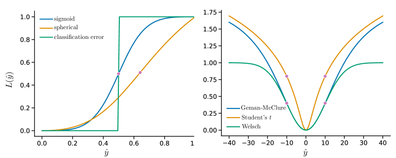
Figure 3: A few nonconvex loss functions for binary classification (left panel) and regression (right panel). In both case the true label/response is $y=0$. For smooth losses, purple dots denote inflexion points: the frontier between the concave part of the loss (that corresponds to “right” predictions) and the concave one (that corresponds to “wrong” ones).

Most of these smooth nonconvex loss functions share the informal property that the loss is locally convex in parts of the prediction space where predictions are “right,” and locally concave in parts where they are “wrong”. We have remained so far voluntarily vague regarding what we meant by “right” and “wrong,” because these terms will have different precise meanings depending on the loss functions. To illustrate this general behavior, let us look at a few examples.

We begin with losses designed for classification, and consider for simplicity the binary case. We assume that the correct class is $y=0$, and the prediction can be either an estimated probability $\hat{y}\in[0,1]$ that $1$ is the correct class, or a real-valued score $\hat{y}\in\mathbb{R}$ that is higher when the classifier is more confident that the label is $1$. We describe below three recipes for designing nonconvex smooth losses, and plot examples in Fig. 3.

• Smooth approximations of the classification error have been used as surrogates of it, and are generally nonconvex. An important instance is the sigmoid loss. This sigmoid loss was popularised by its use within the DOOM II algorithm of Mason et al. (1999). It was also notably studied by Bartlett et al. (2006, Example 7), who showed it was classification-calibrated. This loss is easier to interpret in the probabilistic prediction setting, when $\hat{y}\in[0,1]$. Indeed, in this case, the sigmoid loss is locally convex when $\hat{y}<0.5$, i.e., when the prediction using a 50% threshold is correct, and locally concave when $\hat{y}>0.5$, i.e. when the prediction using the same threshold is wrong. The Savage loss introduced in a boosting context by Masnadi-Shirazi and Vasconcelos (2008) and the normalised cross entropy used by Ma et al. (2020) to train deep nets with noisy labels have a similar sigmoidal shape. They also share the same property of being convex when $\hat{y}<0.5$, and concave when $\hat{y}>0.5$. For these losses, a “right prediction” is one whose most probable class is the correct one. In an opposite fashion, a“wrong prediction” gives the highest probability to the wrong class.

• Scoring rules are the most common way to design losses in the probabilistic setting (when $\hat{y}\in[0,1]$). Most strictly proper scoring rules for classification are convex, with the notable exception of the spherical score (see, e.g., Gneiting and Raftery, 2007). Like the sigmoid loss, the spherical score is convex when $\hat{y}$ is small and concave when $\hat{y}$ is large. However, unlike the sigmoid whose inflection point was at $\hat{y}=50\%$, the spherical inflection point of is at $\hat{y}=1/8+\sqrt{17}/8\approx 64\%$. We give a formal definition in Appendix B. For the spherical loss, a “right prediction” is thus one that will predict the true label $y=0$ using the somewhat peculiar cutoff of $0.64\%$ instead of the usual $50\%$. This illustrates the asymmetry of the spherical score.

• One way to avoid overfitting is to use a loss function that makes the model pay a price for overconfident predictions (potentially even correct ones). This is the rationale behind the tangent loss, introduced by Masnadi-Shirazi et al. (2010) as a boosting objective. Since this is not a probabilistic loss, predictions are real-valued scores $\hat{y}\in\mathbb{R}$. The tangent loss is concave when $\hat{y}$ is either too large or to small, penalising both overconfident mistakes and successes. In this case, “right predictions” correspond to the ones that are not overconfident.

Regarding regression, the most commonly occurring nonconvex smooth losses are used to induce robustness to outliers. The main motivation for such losses is that the squared loss will typically make the model pay an extremely large price for large errors. A way to fix this behavior is to design losses that resemble the squared error when errors are small, but grow less steadily when errors are large. The most famous robust loss is Huber’s (1964), which is equal to the squared error when the error is below a threshold, and grows linearly when the error is above this threshold. Huber’s loss is convex, therefore the analysis of the previous section guarantees that ensembles will get better all the time. However, many other losses that follow this rationale are nonconvex. A nice overview of these robust regression losses was recently offered by Barron (2019), who introduced a new general loss that generalises many previous losses (both convex and nonconvex). All nonconvex losses encompassed by Barron’s generalisation (as well as others, such as using a Student’s $t$ likelihood) share the property of being convex when the error $(\hat{y}-y)^{2}$ is smaller than a prespecified threshold $c$, and nonconvex when the error is larger than $c$. For all these nonconvex losses “bad predictions” are therefore outliers and “good” ones correspond to inliers. A few of these robust losses are displayed on Figure 3, all of them were chosen in order to have a cutoff of $c=10$.

Motivated by the previous examples, we will study a general loss that is smooth, strictly convex in some part of the prediction set $C$ (in that part, the loss Hessian will be positive definite), and strictly concave in another part of $C$ (in that part, the loss Hessian will be negative definite). The following result shows that ensembles will eventually keep getting better when the average prediction $\overline{y}_{\infty}$ ends up in this “good” part (i.e., where $L$ is strictly convex), and will keep getting worse when it ends up in the “bad” part (i.e. where $L$ is strictly concave).

Theorem 5 (Monotonicity of smooth nonconvex losses).

Let $\hat{y}_{1},\ldots,\hat{y}_{K}\in C$ be nondegenerate i.i.d. random variables whose first 5 moments are finite, and $L$ be a function with continuous and bounded partial derivatives of order up to 5, with Hessian matrix $H$. Then

1. If $H(\overline{y}_{\infty})\succ 0$, then the ensemble is eventually getting better: for $K$ large enough,

   $$\mathbb{E}\left[L\left(\overline{y}_{K}\right)\right]<\mathbb{E}\left[L\left(\overline{y}_{K-1}\right)\right],$$ (19)

2. If $H(\overline{y}_{\infty})\prec 0$, then the ensemble is eventually getting worse: for $K$ large enough,

   $$\mathbb{E}\left[L\left(\overline{y}_{K}\right)\right]>\mathbb{E}\left[L\left(\overline{y}_{K-1}\right)\right].$$ (20)

The proof of Theorem 5 is available in Appendix C, and essentially relies on a fourth order Taylor expansion of the loss.

Does this result says something about the classification error?

As illustrated in Figure 3, the sigmoid loss can be seen as a smooth approximation of the classification error. Thus, we could expect that the classification error will behave in the same way: ensembles whose prediction are eventually correct keep getting better, and ensembles who are eventually wrong keep getting worse. One might even contemplate the idea of an easy proof using the fact that the classification error is a limiting case of a sigmoid loss. Unfortunately, we did not manage to make such a proof work, and the behavior of the classification error is considerably more subtle, and involves more complex regularity conditions than the smoothness and moment assumptions of Theorem 5.

4.2 Why is the classification error difficult to handle?

To understand why the classification error is much more difficult to study than smooth losses, it is interesting to look at the following (counter) example, that goes back to Condorcet (1785), and was studied thoroughly by Lam and Suen (1997).

Consider a binary classification classification task, where the true label is $0$, and our predictions $\hat{y}_{1},\cdots,\hat{y}_{K}$ are i.i.d. samples from a Bernoulli distribution $\mathcal{B}(\overline{y}_{\infty})$. In that case, the classification error of any $\hat{y}\in[0,1]$ is simply $L(\hat{y})=\mathbf{1}(\hat{y}\leq 0.5)$. The expected loss of the ensemble will therefore be $\mathbb{E}[L(\overline{y}_{k})]=\mathbb{P}(\overline{y}_{K}\leq 0.5)$. It seems reasonable to conjecture that $\mathbb{P}(\overline{y}_{K}\leq 0.5)$ will go to zero decreasingly when $\overline{y}_{\infty}>0.5$, and to one increasingly when $\overline{y}_{\infty}<0.5$, which would be consistent with the analogy to the sigmoid loss sketched above. Unfortunately, this is not the case, and $\mathbb{P}(\overline{y}_{K}\leq 0.5)$ is not, in general, monotonic (even asymptotically).

Indeed, let us focus for instance on the case where the ensemble is eventually right, i.e., when $\overline{y}_{\infty}<0.5$. In that case, it can be shown that the subsequence of ensembles containing an odd number of models $L(\overline{y}_{2K+1})$ decreases (see Shteingart et al., 2020, Theorem 2, for a proof). However, monotonicity is broken when we include even numbers of models (Lam and Suen, 1997). A heuristic explanation of this failure, already mentioned by Condorcet (1785), is that odd numbers of predictions allow ties. Probst and Boulesteix (2018, Section 3.1.1) discuss this problem of ties as well, and possible tie-breakers.

This counterexample shows that an example as benign as a Bernoulli distribution is problematic for the classification error, and that a more complex mathematical machinery than the one of the previous proofs is required. tex

We develop such a machinery in the next section, leveraging large deviation theorems to study the monotonicity of quantities such as $\mathbb{P}(\overline{y}_{K}\leq 0.5)$. This section is largely independent from the rest of the paper, since it may be of independent interest, beyond ensembles.

4.3 Monotonicity of tail probabilities

In this section, we present two results on the monotonicity of tail probabilities of empirical means. We state these results in a general form, since they may be of broader interest. Namely, we consider a sequence of i.i.d. random variables $X_{1},\ldots,X_{n}$ living in $\mathbb{R}^{D}$ with finite expectation $\mu\in\mathbb{R}^{D}$.

Our goal is to find under which conditions $\operatorname{\mathbb{P}}\left(\overline{X}_{n}\geq\mu+\varepsilon\right)$ is eventually strictly decreasing, for a given $\varepsilon>0$. We know that $\operatorname{\mathbb{P}}\left(\overline{X}_{n}\geq\mu+\varepsilon\right)$ converges to zero without additional assumptions (this is a consequence of the weak law of large numbers). We will first deal with the univariate case (Theorem 6), for which more intuitive regularity conditions are available than for the general, multivariate setting (Theorem 7). In the next section, we will be able to readily apply these results to the sequence of predictions $\hat{y}_{k}$ to obtain an analogous of Theorem 5 for the classification error.

Theorem 6 (monotonicity of tail probabilities, univariate).

Let $X_{1},\ldots,X_{n}$ be i.i.d. random variables with finite expectation $\mu$, and let $\varepsilon>0$. Assume furthermore that

1. $\operatorname{\mathbb{E}}\left[\operatorname{e}^{tX_{1}}\right]<+\infty$ for all $t\in\mathbb{R}$;

2. $\operatorname{\mathbb{P}}\left(X_{1}>\mu+\varepsilon\right)>0$;

3. $X_{1}$ is absolutely continuous with respect to the Lebesgue measure;

or, alternatively to (3),

1. $X_{1}$ is a lattice random variable and $\operatorname{\mathbb{P}}\left(X_{1}=\mu+\varepsilon\right)>0$.

Then, $\operatorname{\mathbb{P}}\left(\overline{X}_{n}\geq\mu+\varepsilon\right)$ and $\operatorname{\mathbb{P}}\left(\overline{X}_{n}>\mu+\varepsilon\right)$ are both strictly decreasing for all $n$ large enough.

The idea of the proof (which can be found in Section D of the Appendix) is to use precise asymptotic results on tail probabilities obtained by Petrov (1965) (see also Bahadur and Ranga Rao, 1960). These results are sometimes referred to as “sharp” or “strong” large deviation theorems (because they are more precise than standard large deviations results like Cramer’s celebrated theorem).

We want to emphasize that Theorem 6, while intuitive, may not hold if $X_{1}$ does not meet the assumptions outlined in the statement of Theorem 6. As a first example, let us assume that $X_{1}$ has a $\alpha$-stable distribution with $\alpha<1$. Then one can show that $\operatorname{\mathbb{P}}\left(\overline{X}_{n}>\mu+\varepsilon\right)$ is actually increasing (see Section E of the Appendix). Of course, taking $\alpha<1$ in this example prevents $X_{1}$ from having finite expectation. Another intriguing example, sketched in the previous subsection, is when $X_{1}\sim\mathcal{B}(\mu)$ with $\mu\in(0,1)$. In that case, one can also derive the exact distribution of $X_{1}+\cdots+X_{n}$, a binomial $\mathrm{Bin}(n,\mu)$. Thus $\operatorname{\mathbb{P}}\left(\overline{X}_{n}>\mu+\varepsilon\right)$ can be written as a sum of binomial coefficients, whose behavior is notoriously difficult to fully comprehend (see e.g. Lam and Suen (1997), who show non-monotonicity in some cases). Here it is assumption (3bis) which does not hold: there is no mass at $\mu+\varepsilon$. As we illustrate in Appendix E, adding a small mass at $\mu+\varepsilon$ restores monotonicity. Coming back to the counter example of Section 4.2, which corresponds to the case $\mu+\varepsilon=0.5$, this means that allowing models to make no decision (i.e. outputting $\hat{y}=0.5$ with nonzero probability) leads to monotonicity in the classical Condorcet setting. Intuitively, this can be interpreted as follows: allowing blank votes make ties possibles both when there is an odd or an even number of voters. It is quite interesting to see here the classical regularity conditions of Bahadur and Ranga Rao (1960) and Petrov (1965) explain neatly the mathematical origins of the problem of even voters in Condorcet’s theorem.

Now we present a multivariate extension of Theorem 6. Note that, from now on, when $u$ and $v$ are both vectors, $u\leq v$ means that $u_{i}\leq v_{i}$ for all indices.

Theorem 7 (Monotonicity of tails, multivariate).

Let $X_{1},\ldots,X_{n}\in\mathbb{R}^{D}$ be i.i.d. random vectors distributed as $X$, finite mean $\mu$, moment-generating function $\phi:t\mapsto\operatorname{\mathbb{E}}\left[\mathrm{exp}\left(\langle t,X_{1}\rangle\right)\right]$, and cumulant-generating function $\varphi=\log\phi$. Assume that

1. $X$ has density $\rho$ with respect to the Lebesgue measure on $\mathbb{R}^{D}$ and that $\rho$ does not cancel;

2. there exists $\alpha>0$ such that $\phi$ is differentiable and bounded on $U_{\alpha}$, the open ball of radius $\alpha$

3. there exists constants $0<\lambda_{\min}<\lambda_{\max}<+\infty$ such that $\mathrm{Spec}(\nabla^{2}\varphi)\subseteq[\lambda_{\min},\lambda_{\max}]$.

Then, for any $\varepsilon\in\mathbb{R}^{D}$ such that $\varepsilon>0$ and

$$\min_{i\leq D}\frac{\varepsilon_{i}}{\left\lVert\varepsilon\right\rVert}<\sqrt{\frac{\lambda_{\min}}{\lambda_{\max}}}\,,$$ (21)

it holds that $\operatorname{\mathbb{P}}\left(\overline{X}_{n}\geq\mu+\varepsilon\right)$ is decreasing for $n$ large enough.

Theorem 7 is proved in Appendix D.2. In some sense, it generalises Theorem 6, since dealing with multivariate summands (which will allow us to treat the multiclass classification error in the next section). However, this comes at the cost of more stringent assumptions on the distribution of $X$, and in particular the local behavior of its cumulative distribution function. Moreover, while Theorem 6 was also applicable to some lattice random variables, this multivariate Theorem is restricted to absolutely continuous distributions. In particular, this means that $\operatorname{\mathbb{P}}\left(\overline{X}_{n}>\mu+\varepsilon\right)=\operatorname{\mathbb{P}}\left(\overline{X}_{n}\geq\mu+\varepsilon\right)$ is also eventually decreasing.

4.4 Ensembles and the classification error

We are finally in position to deal with the classification error. We consider a classification problem with $n_{\text{Cl}}$ classes. The true label is $y\in\{0,1\}^{n_{\text{Cl}}}$, and a prediction is a $n_{\text{Cl}}$-dimensional vector $\hat{y}=(\hat{y}^{(c)})_{c\leq n_{\text{Cl}}}\in\mathbb{R}^{n_{\text{Cl}}}$ of scores (that can be, for instance, estimated probabilities of each class). Without loss of generality, we assume that the true class is the first one ($y=(1,0,\ldots,0)^{\top}$). The classification error is then equal to one whenever the score of the true class is smaller than the maximum score:

$$L(\hat{y})=\left\{\begin{matrix}1\;\text{ if }\;\hat{y}^{(1)}\leq\text{max}_{c\neq 1}\left(\hat{y}^{(c)}\right)\\ 0\;\text{ if }\;\hat{y}^{(1)}>\text{max}_{c\neq 1}\left(\hat{y}^{(c)}\right).\end{matrix}\right.$$ (22)

The expected loss of an ensemble will thus be $\mathbb{E}[L(\overline{y}_{K})]=\mathbb{P}\left({\overline{y}_{K}}^{(1)}\leq\text{max}_{c\neq y}{\overline{y}_{K}}^{(c)}\right)$, which looks like something that could be attacked with the tail probability theorems of the previous section. And indeed it can, by rewriting the classification error

$$\mathbb{E}[L(\overline{y}_{K})] =1-\mathbb{P}\left({\overline{y}_{K}}^{(1)}>\max_{c\neq 1}{\overline{y}_{K}}^{(c)}\right)$$

$$=1-\mathbb{P}\left({\overline{y}_{K}}^{(1)}>{\overline{y}_{K}}^{(2)},\ldots,{\overline{y}_{K}}^{(1)}>{\overline{y}_{K}}^{(n_{\text{Cl}})}\right)$$

$$=1-\mathbb{P}\left({\overline{y}_{K}}^{(1)}1_{n_{\text{Cl}}-1}-{\overline{y}_{K}}^{(-1)}>0\right)$$

$$=1-\mathbb{P}\left(\frac{1}{K}\sum_{k=1}^{K}\left(\hat{y}_{k}^{(1)}1_{n_{\text{Cl}}}-{\hat{y}_{k}}^{(-1)}\right)>0\right)$$

$$=1-\mathbb{P}\left(\overline{X}_{K}>0\right)$$

$$=\mathbb{P}\left(-\overline{X}_{K}\geq 0\right),$$

where $1_{n_{\text{Cl}}-1}\in\mathbb{R}^{n_{\text{Cl}}-1}$ is a vector of ones, ${\hat{y}_{k}}^{(-1)}=\left({\hat{y}_{k}}^{(2)},\ldots,{\hat{y}_{k}}^{(n_{\text{Cl}})}\right)$ is the $(n_{\text{Cl}}-1)$-dimensional vector of the scores of the wrong classes, and, for all $k\in\{1,\ldots,K\}$,

$$X_{k}={\hat{y}_{k}}^{(1)}1_{n_{\text{Cl}}-1}-{\hat{y}_{k}}^{(-1)}\in\mathbb{R}^{n_{\text{Cl}}-1}.$$ (23)

In the binary case, when $n_{\text{Cl}}=2$, $X_{k}={\hat{y}_{k}}^{(1)}-{\hat{y}_{k}}^{(2)}$ just corresponds to the margin, that is, the difference between the score of the correct label and the score of the incorrect one.. In the multiclass case, $X_{k}$ is a $(n_{\text{Cl}}-1)$-dimensional vector of margins obtained for each possible “1 versus $c$” classification problems, for $c\in\{2,\ldots,n_{\text{Cl}}\}$. Following the seminal work of Bartlett et al. (1998), margins have been used a lot to study the theory of ensembles (see, e.g., Biggs et al., 2022, and references therein).

Before we state our theorem, we have to translate to the ensemble framework the regularity conditions of the two theorems of Section 4.3. We will provide two sets of assumptions that we cover the binary classification case (related Theorem 6) and the general multiclass setting (related to Theorem 7). In the rest of this section, we assume that $\hat{y}_{1},\ldots,\hat{y}_{k}\in\mathbb{R}^{n_{\text{Cl}}}$ are i.i.d. random variables with finite mean $\overline{y}_{\infty}$.

Assumption 1 (Correct prediction).

Let $\varepsilon=\mathbb{E}[X_{1}]={\overline{y}_{\infty}}^{(1)}1_{n_{\text{Cl}}-1}-{\overline{y}_{\infty}}^{(-1)}$. There are either $n_{\text{Cl}}=2$ classes and the regularity conditions of Theorem 6 are verified, or there are $n_{\text{Cl}}>2$ classes and the regularity conditions of Theorem 7 are verified, for $-X_{1},\ldots,-X_{K}$ and $\varepsilon$.

Assumption 1 implies in particular that $\varepsilon=\mathbb{E}[X_{1}]>0$ which is equivalent to the fact that the expected margin ${\overline{y}_{\infty}}^{(1)}-\max_{c\neq 1}{\overline{y}_{\infty}}^{(c)}$ is positive, and to the fact that the asymptotic prediction is correct, that is, $L(\overline{y}_{\infty})=0$. This assumption of positive margin is often used to study ensembles (see, e.g., Breiman, 2001).

Assumption 2 (Completely incorrect prediction).

Let $\varepsilon=-\mathbb{E}[X_{1}]={\overline{y}_{\infty}}^{(-1)}-{\overline{y}_{\infty}}^{(1)}1_{n_{\text{Cl}}-1}$. There are either $n_{\text{Cl}}=2$ classes and the regularity conditions of Theorem 6 are verified, or there are $n_{\text{Cl}}>2$ classes and the regularity conditions of Theorem 7 are verified, for $X_{1},\ldots,X_{K}$ and $\varepsilon$.

Assumption 2 implies in particular that $\varepsilon=-\mathbb{E}[X_{1}]>0$, which means that all margins are negative, i.e. that the model asymptotically gives the lowest score to the true class. Because of this, we call this an assumption of completely incorrect prediction. This implies in particular that $L(\overline{y}_{\infty})=1$.

Theorem 8 (Monotonicity of the classification error).

Let $\hat{y}_{1},\ldots,\hat{y}_{K}\in\mathbb{R}^{n_{\text{Cl}}}$ be i.i.d. random variables. Then

1. If the prediction is asymptotically correct (Assumption 1), then the ensemble is eventually getting better: for $K$ large enough,

   $$\mathbb{E}\left[L\left(\overline{y}_{K}\right)\right]<\mathbb{E}\left[L\left(\overline{y}_{K-1}\right)\right],$$ (24)

2. If the prediction is asymptotically completely incorrect (Assumption 2), then the ensemble is eventually getting better: for $K$ large enough,

   $$\mathbb{E}\left[L\left(\overline{y}_{K}\right)\right]>\mathbb{E}\left[L\left(\overline{y}_{K-1}\right)\right].$$ (25)

Proof  We begin by assuming that the prediction is correct (Assumption 1). Then, Theorem 6 (when $n_{\text{Cl}}=2$) or Theorem 7 (when $n_{\text{Cl}}>2$) ensures that $\operatorname{\mathbb{P}}\left(-\overline{X}_{n}\geq-\mathbb{E}[X_{1}]+\varepsilon\right)=\operatorname{\mathbb{P}}\left(-\overline{X}_{n}\geq 0\right)$ decreases for $K$ large enough. Using Eq. (4.4), this implies that $L(\overline{y}_{\infty})$ eventually decreases.

We now deal with the case of an incorrect prediction (Assumption 2). Again, Theorem 6 or Theorem 7 ensures that $\operatorname{\mathbb{P}}\left(\overline{X}_{n}>\mathbb{E}[X_{1}]+\varepsilon\right)=\operatorname{\mathbb{P}}\left(\overline{X}_{n}>0\right)$ eventually decreases. In turn, $L(\overline{y}_{\infty})$ eventually increases.  

5 Conclusion

Our initial question was “Is it always true that an ensemble of $K+1$ models performs better than an ensemble of $K$ models?” When the loss is convex and the ordering of the ensemble does not matter, Theorems 2 and 4 provide a clear and positive answer to this question. When the loss is non-convex, however, a more nuanced picture must be drawn: ensembles will get better in some setting, and worse in others.

Acknowledgments and Disclosure of Funding

This work was supported by the French government, through the 3IA Côte d’Azur Investments in the Future project managed by the National Research Agency (ANR) with the reference number ANR-19-P3IA-0002. DG also acknowledges the support of ANR through project NIM-ML (ANR-21-CE23-0005-01) and of EU Horizon 2020 project AI4Media (contract no. 951911).

Appendix A Proof of strict improvements under strong convexity

We prove here Theorem 4. Strong convexity leads to the following strengthening of Jensen’s inequality (see, e.g., Nikodem, 2014, Theorem 2).

Theorem 9 (Jensen improvement).

If $L:C\rightarrow\mathbb{R}$ is $\mu$-strongly convex, then, for all $x_{1},\ldots,x_{K}$, and

$$\small L\left(\frac{1}{K}\sum_{k=1}^{K}x_{k}\right)\leq\frac{1}{K}\sum_{k=1}^{K}L\left(x_{k}\right)-\mu\frac{1}{K}\sum_{k=1}^{K}\left|\left|x_{k}-\frac{1}{K}\sum_{j=1}^{K}x_{j}\right|\right|^{2}.$$ (26)

Our goal is to combine this result with our basic identity Eq. (8) to prove Theorem 4. We use Theorem 9 with $x_{j}=\frac{1}{K-1}\sum_{k\neq j}\hat{y}_{k}$. Using Eq. (8) and the exchangeability assumption, we find that

$$\mathbb{E}\left[L\left(\frac{1}{K}\sum_{k=1}^{K}\hat{y}_{k}\right)\right]\leq\mathbb{E}\left[L\left(\frac{1}{K-1}\sum_{k=1}^{K-1}\hat{y}_{k}\right)\right]-\mu\mathbb{E}\left[\left|\left|\frac{1}{K-1}\sum_{k=1}^{K-1}\hat{y}_{k}-\frac{1}{K}\sum_{k=1}^{K}\hat{y}_{k}\right|\right|^{2}\right].$$ (27)

We can then compute the expectation on the right-hand side

$$\mathbb{E}\left[\left|\left|\frac{1}{K-1}\sum_{k=1}^{K-1}\hat{y}_{k}-\frac{1}{K}\sum_{k=1}^{K}\hat{y}_{k}\right|\right|^{2}\right] =\frac{1}{K^{2}(K-1)^{2}}\mathbb{E}\left[\left|\left|K\sum_{k=1}^{K-1}\hat{y}_{k}-(K-1)\left(\hat{y}_{K}+\sum_{k=1}^{K-1}\hat{y}_{k}\right)\right|\right|^{2}\right]$$

$$=\frac{1}{K^{2}(K-1)^{2}}\mathbb{E}\left[\left|\left|\sum_{k=1}^{K-1}\hat{y}_{k}-(K-1)\hat{y}_{K}\right|\right|^{2}\right]$$

$$=\frac{1}{K^{2}(K-1)^{2}}\textup{tr}\left(\textup{Cov}\left(\sum_{k=1}^{K-1}\hat{y}_{k}-(K-1)\hat{y}_{K}\right)\right).$$ (28)

We can now use Bienaymé’s identity and exchangeability to compute the trace of the covariance:

$$\textup{tr}\left(\textup{Cov}\left(\sum_{k=1}^{K-1}\hat{y}_{k}-(K-1)\hat{y}_{K}\right)\right)=(K-1)\textup{tr}\left(\Sigma\right)+(K-1)(K-2)\textup{tr}\left(\textup{Cov}\left(\hat{y}_{1},\hat{y}_{2}\right)\right)\\ +(K-1)^{2}\textup{tr}\left(\Sigma\right)-2\textup{tr}\left(\textup{Cov}\left(\sum_{k=1}^{K-1}\hat{y}_{k},(K-1)\hat{y}_{K}\right)\right),$$ (29)

finally leading to

$$\textup{tr}\left(\textup{Cov}\left(\sum_{k=1}^{K-1}\hat{y}_{k}-(K-1)\hat{y}_{K}\right)\right)=K(K-1)\textup{tr}(\Sigma)(1-\rho)\,.$$ (30)

Plugging this expression into Equation (28) gives the desired bound. $\blacksquare$

Appendix B More details on the spherical score

Consider the setting of Section 4.1. The spherical score is defined as

$$L_{1}(\hat{y})=-\frac{\hat{y}}{\sqrt{\hat{y}^{2}+(1-\hat{y})^{2}}}\,,$$ (31)

when the true label is $y=1$. When the true label is $0$, as in Section 4.1, it is defined as

$$L_{0}(\hat{y})=-\frac{1-\hat{y}}{\sqrt{\hat{y}^{2}+(1-\hat{y})^{2}}}.$$ (32)

The second derivative of $L_{0}$ is $\hat{y}\mapsto(-4\hat{y}^{2}+\hat{y}+1)/(2(\hat{y}-1)x+1)^{5/2}$, whose unique root in $[0,1]$ is $1/8+\sqrt{17}/8\approx 0.64$. Therefore, as seen in Figure 3, $L_{0}$ will be strictly convex on $[0,1/8+\sqrt{17}/8)$ and strictly concave on $(1/8+\sqrt{17}/8,1]$.

Appendix C Proof of the theorem for smooth losses (Theorem 5)

We only treat the case $H(\hat{y}_{\infty})\succ 0$, since the case $H(\hat{y}_{\infty})\prec 0$ follows by replacing $L$ by $-L$. We will base our proof on the following lemma, which is obtained by Taylor-expanding the loss up to the fourth order. In this context, such a technique is often called the delta method for moments (see, e.g., Small, 2010; Bickel and Doksum, 2015). The proof of the lemma is slightly tedious, and is provided after the main theorem.

Lemma 10 (fourth order delta method).

Let $X_{1},\ldots,X_{n}$ be a sequence of i.i.d. random variables whose first $5$ moments are finite, with mean $\mu$ and covariance matrix $\Sigma\succeq 0$. Let $L$ be a function with continuous and bounded partial derivatives of order up to 5, with Hessian matrix $H$. Then, there exists a constant $\alpha\in\mathbb{R}$, that depends on the first $3$ moments of $X$ and the partial derivatives of the loss of order up to $4$, such that, when $K$ goes to infinity

$$\mathbb{E}[L(\bar{X}_{K})]=L(\mu)+\frac{\textup{tr}(H(\mu)\Sigma)}{2K}+\frac{\alpha}{K^{2}}+\mathcal{O}\left(\frac{1}{K^{5/2}}\right)\,.$$ (33)

Applying this result successively to $\bar{y}_{K}$ and $\bar{y}_{K+1}$ and taking the difference between the two terms, we obtain

$$\mathbb{E}[L(\bar{y}_{K})]-\mathbb{E}[L(\bar{y}_{K+1})] =\frac{\textup{tr}(H(\hat{y}_{\infty})\Sigma)}{2}\left(\frac{1}{K}-\frac{1}{K+1}\right)+\alpha\left(\frac{1}{K^{2}}-\frac{1}{(K+1)^{2}}\right)+\mathcal{O}\left(\frac{1}{K^{5/2}}\right)$$ (34)

$$=\frac{\textup{tr}(H(\hat{y}_{\infty})\Sigma)}{2}\frac{1}{K(K+1)}+\alpha\frac{1+2K}{K^{2}(K+1)^{2}}+\mathcal{O}\left(\frac{1}{K^{5/2}}\right).$$ (35)

Therefore,

$$K(K+1)\left(\mathbb{E}[L(\bar{y}_{K})]-\mathbb{E}[L(\bar{y}_{K+1})]\right) =\frac{\textup{tr}(H(\hat{y}_{\infty})\Sigma)}{2}+\alpha\frac{1+2K}{K(K+1)}+\mathcal{O}\left(\frac{1}{K^{1/2}}\right),$$ (36)

which implies that $K(K+1)\left(\mathbb{E}[L(\bar{y}_{K})]-\mathbb{E}[L(\bar{y}_{K+1})]\right)$ will converge to $\textup{tr}(H(\hat{y}_{\infty})\Sigma)/2$ when $K$ goes to infinity. Therefore, for $K$ large enough, the sign of $\mathbb{E}[L(\bar{y}_{K})]-\mathbb{E}[L(\bar{y}_{K+1})]$ is constant and exactly equal to the sign of $\textup{tr}(H(\hat{y}_{\infty})\Sigma)$.

Since $H(\hat{y}_{\infty})\succ 0$, $\Sigma\succeq 0$, and $\Sigma\neq 0$, a standard property of symmetric matrices (see, e.g., Serre, 2010, Proposition 6.1) ensures that $H(\hat{y}_{\infty})\Sigma$ is diagonalisable, with only real nonnegative eigenvalues (at least one of them being positive). This implies that $\textup{tr}(H(\hat{y}_{\infty})\Sigma)>0$, and, in turn, that for $K$ large enough, $\mathbb{E}[L(\bar{y}_{K+1})]<\mathbb{E}[L(\bar{y}_{K})]$. ∎

C.1 Proof of the fourth order delta method (Lemma 10)

Lemma 10 was proven in the univariate case by Small (2010, Section 4.3) and we extend it here to the multivariate case. We will see it as a consequence of the multivariate version of delta method presented by Bickel and Doksum (2015).

Under the assumptions of Lemma 10, Theorem 5.3.2 of Bickel and Doksum (2015) implies

$$\mathbb{E}[L(\bar{X}_{K})]=L(\mu)+\sum_{r=2}^{4}\frac{1}{r!}\sum_{j_{1},j_{2},\ldots,j_{r}=1}^{d}\frac{\partial^{r}L}{\partial x_{j_{1}}\cdots\partial x_{j_{r}}}(\mu)\mathbb{E}[(\bar{X}_{Kj_{1}}-\mu_{j_{1}})\cdots(\bar{X}_{Kj_{r}}-\mu_{j_{r}})]+\mathcal{O}(K^{-5/2})\,.$$ (37)

Let us look at the quadratic term. We have

$$\frac{1}{2}\sum_{j_{1},j_{2}=1}^{d}\frac{\partial^{2}L}{\partial x_{j_{1}}\partial x_{j_{2}}}(\mu)\mathbb{E}[(\bar{X}_{Kj_{1}}-\mu_{j_{1}})(\bar{X}_{Kj_{2}}-\mu_{j_{2}})] =\frac{1}{2}\mathbb{E}\left[(\bar{X}_{K}-\mu)^{T}H(\mu)(\bar{X}_{K}-\mu)\right]$$ (38)

$$=\frac{1}{2}\textup{tr}(H(\mu)\textup{Cov}(\bar{X}_{K}))=\frac{\textup{tr}(H(\mu)\Sigma)}{2K}.$$ (39)

Let us now look at the third and fourth order terms. We need to assess how $K$ affects the multivariate moments of the empirical mean. Let us define first the multivariate moments of $X$ as, for $r\in\{3,4\}$ and $j_{1},\ldots,j_{r}\in\{1,\ldots,d\}$

$$\mu_{j_{1},\ldots,j_{r}}=\mathbb{E}[(X_{j_{1}}-\mu_{j_{1}})\ldots(X_{j_{r}}-\mu_{j_{r}})]\,,$$ (40)

The moments of $\bar{X}_{K}$ can now be expressed in terms of moments of $X$. Following for instance Hall (1992, p. 54) or McCullagh (2018, Section 2.3), we have

$$\mathbb{E}[(\bar{X}_{Kj_{1}}-\mu_{j_{1}})(\bar{X}_{Kj_{2}}-\mu_{j_{2}})(\bar{X}_{Kj_{3}}-\mu_{j_{3}})]=\frac{1}{K^{2}}\mu_{j_{1},j_{2},j_{3}}\,,$$ (41)

and

$$\mathbb{E}[(\bar{X}_{Kj_{1}}-\mu_{j_{1}})(\bar{X}_{Kj_{2}}-\mu_{j_{2}})(\bar{X}_{Kj_{3}}-\mu_{j_{3}})(\bar{X}_{Kj_{4}}-\mu_{j_{4}})]=\frac{\mu_{j_{1},j_{2}}\mu_{j_{3},j_{4}}+\mu_{j_{1},j_{3}}\mu_{j_{2},j_{4}}+\mu_{j_{1},j_{4}}\mu_{j_{2},j_{3}}}{K^{2}}+\mathcal{O}\left(\frac{1}{K^{3}}\right),$$ (42)

where the constant in the $\mathcal{O}$ is a multivariate cumulant. Plugging these expressions into Equation (37) finally gives

$$\mathbb{E}[L(\bar{X}_{K})]=L(\mu)+\frac{\textup{tr}(H(\mu)\Sigma)}{2K}+\frac{\alpha}{K^{2}}+\mathcal{O}\left(\frac{1}{K^{5/2}}\right),$$ (43)

with

$$\alpha=\frac{1}{3!}\sum_{j_{1},j_{2},j_{3}=1}^{d}\frac{\partial^{3}L}{\partial x_{j_{1}}\partial x_{j_{2}}\partial x_{j_{3}}}(\mu)\mu_{j_{1},j_{2},j_{3}}\\ +\frac{1}{4!}\sum_{j_{1},j_{2},j_{3},j_{4}=1}^{d}\frac{\partial^{4}L}{\partial x_{j_{1}}\partial x_{j_{2}}\partial x_{j_{3}}\partial x_{j_{4}}}(\mu)\left(\mu_{j_{1},j_{2}}\mu_{j_{3},j_{4}}+\mu_{j_{1},j_{3}}\mu_{j_{2},j_{4}}+\mu_{j_{1},j_{4}}\mu_{j_{2},j_{3}}\right).$$ (44)

One can check that, in the univariate case ($d=1$), our expression for $\alpha$ is identical to the one given by Small (2010, Section 4.3). ∎

Appendix D Omitted proofs for Section 4.3

D.1 Proof of Theorem 6

For all $i\geq 1$, let us set $Y_{i}\vcentcolon=X_{i}-\mu$. Note that, by definition, the $Y_{i}$s are i.i.d. and centered. We are going to apply Theorem 3 and 6 of Petrov (1965) to the random variables $Y_{i}$s. Let us recall briefly Petrov’s results here. We start with some notation: $V(x)$ denotes the cdf of $X_{1}$, $\mathfrak{U}$ denotes the points of increase of $V$ and $A$ its supremum, $\mathcal{B}^{+}$ denotes the set of non-negative values of $h$ such that $\int_{0}^{+\infty}\operatorname{e}^{hx}\mathrm{d}V(x)<+\infty$ and $B$ its supremum. Further, assuming $B>0$, for any $0<h<B$, we define

$$R(h)=\int_{-\infty}^{+\infty}\operatorname{e}^{hx}\mathrm{d}V(x)\,,\qquad m(h)=\frac{1}{R(h)}\int_{-\infty}^{+\infty}x\operatorname{e}^{hx}\mathrm{d}V(x)\qquad\text{and}\qquad\sigma(h)^{2}=\frac{\mathrm{d}m(h)}{\mathrm{d}h}\,.$$

Finally, define $A_{0}=\lim_{h\to B^{-}}m(h)$. We are now able to state the results:

Theorem 11 (Theorem 3 and Theorem 6 from Petrov (1965)).

Let $Y_{1},Y_{2},\ldots$ be a sequence of i.i.d. random variables.

• Assume that the $Y_{i}$s are non-lattice such that $B>0$. Let $c$ be any constant satisfying the condition $\operatorname{\mathbb{E}}\left[Y_{1}\right]<c<A_{0}$. Then

  $$\operatorname{\mathbb{P}}\left(Y_{1}+\cdots+Y_{n}\geq nc\right)=\frac{\exp\left(n\log R(h)-nhc\right)}{h\sigma(h)\sqrt{2\pi n}}(1+o\left(1\right))\,.$$

  Here $h$ is the unique real root of the equation $m(h)=c$.

• Assume that the $Y_{i}$ are lattice distributed with values in $a+NH$, $N\in\mathbb{Z}$. Assume that $\operatorname{\mathbb{E}}\left[Y_{1}\right]>-\infty$, $A_{0}<+\infty$, and $B>0$. If $nx\in na+\mathbb{Z}H$, then

  $$\operatorname{\mathbb{P}}\left(Y_{1}+\cdots+Y_{n}=nx\right)=\frac{H\exp\left(n\log R(h)-nhx\right)}{\sigma(h)\sqrt{2\pi n}}\left(1+\mathcal{O}\left(\frac{1}{n}\right)\right)\,,$$

  and

  $$\operatorname{\mathbb{P}}\left(Y_{1}+\cdots+Y_{n}\geq nx\right)\leq\frac{H\exp\left(n\log R(h)-nhx\right)}{\sigma(h)\sqrt{2\pi n}(1-\operatorname{e}^{-Hh})}\left(1+\mathcal{O}\left(\frac{1}{n}\right)\right)\,$$

  as $n\to+\infty$ uniformly in $x\in[\operatorname{\mathbb{E}}\left[Y_{1}\right]+\varepsilon,A_{0}-\varepsilon]$, with $\varepsilon>0$ arbitrary. Here $h$ is the unique real root of the equation $m(h)=x$.

Theorem 11 gives us a control of the tail probability, which is precise enough to show monotonicity. There are two cases to consider: the non-lattice case (assuming (1), (2), and (3)) and the lattice case (assuming (1), (2), and (3bis)). We denote $p_{n}=\operatorname{\mathbb{P}}\left(\overline{X}_{n}\geq\mu+\varepsilon\right)$, for $\varepsilon$ satisfying the assumptions of the theorem.

Non-lattice case.

Under assumption (3), we know that the $Y_{i}$s are non-lattice random variables. Let us check carefully the assumptions of Petrov’s result: Under assumption (1), we know that $B=+\infty$. Under assumption (2), we know that $\operatorname{\mathbb{P}}\left(Y_{1}>\varepsilon\right)>0$. In the language of Petrov (1965), it implies that there is a growth point of $Y_{1}$ greater than $\varepsilon$. Thus $A$ is greater than $\varepsilon$. Since we are in the case $B=+\infty$, we know that $A_{0}=A$, and in particular $A_{0}>\varepsilon>0$. Thus we can apply the first part of Theorem 11 to the $Y_{i}$s with $c=\varepsilon$. We obtain

$$\forall n\in\mathbb{N}^{\star},\qquad p_{n}=\frac{\mathrm{exp}\left(n\log R(h)-nh\varepsilon\right)}{h\sigma(h)\sqrt{2\pi n}}(1+u_{n})\,,$$ (45)

where $u_{n}=o\left(1\right)$ as $n\to+\infty$. From Eq. (45), we deduce that, for all $n\geq 1$,

$$\frac{p_{n+1}}{p_{n}}=\rho\sqrt{\frac{n}{n+1}}\frac{1+u_{n+1}}{1+u_{n}}\,,$$ (46)

where $\rho\vcentcolon=\mathrm{exp}\left(\log R(h)-h\varepsilon\right)$. By the first lemma in Petrov (1965), $m$ is strictly increasing and continuous in $(0,+\infty)$. Thus, by definition of $h$, the mapping $\alpha:t\mapsto\log R(t)-t\varepsilon$ is decreasing for $t<h$ and increasing for $t>h$, attaining a (strict) minimum in $t=h$. Since $\alpha(0)=0$, we deduce that $\alpha(h)<0$, which in turn implies $\rho<1$ in Eq. (46). Since both $\sqrt{n/(n+1)}$ and $(1+u_{n+1})/(1+u_{n})$ are arbitrarily close to $1$ for large $n$, we deduce the result in the case of a non-lattice distribution.

Lattice case.

As in the previous paragraph, under assumption (1) and (2), $B=+\infty$ and $A_{0}>\varepsilon>0$. Moreover, assumption (3bis) guarantees that $n\varepsilon$ takes values in the lattice. Similarly to Eq. (45), we obtain

$$\forall n\in\mathbb{N}^{\star},\qquad p_{n}=\frac{H\mathrm{exp}\left(n\log R(h)-nh\varepsilon\right)}{\sigma(h)\sqrt{2\pi n}(1-\operatorname{e}^{-Hh})}(1+u_{n})\,,$$ (47)

where $u_{n}=o\left(1\right)$. From Eq. (49), we deduce that, for all $n\geq 1$,

$$\frac{p_{n+1}}{p_{n}}=\rho\sqrt{\frac{n}{n+1}}\frac{1+u_{n+1}}{1+u_{n}}\,,$$ (48)

where $\rho$ is as before. We conclude in the same fashion as in the first part of the proof and obtain monotonicity for $\operatorname{\mathbb{P}}\left(\overline{X}_{n}\geq\mu+\varepsilon\right)$.

Let us now deal with the strict inequality case. Decomposing $\operatorname{\mathbb{P}}\left(\overline{X}_{n}>\mu+\varepsilon\right)$ as the difference between $\operatorname{\mathbb{P}}\left(\overline{X}_{n}\geq\mu+\varepsilon\right)$ and $\operatorname{\mathbb{P}}\left(\overline{X}_{n}=\mu+\varepsilon\right)$, and using again Theorem 11, we obtain

$$\operatorname{\mathbb{P}}\left(\overline{X}_{n}>\mu+\varepsilon\right)=\frac{H\mathrm{exp}\left(n\log R(h)-nh\varepsilon\right)}{h\sigma(h)\sqrt{2\pi n}}\left(\frac{1}{1-\operatorname{e}^{-Hh}}-1\right)(1+u_{n})\,,$$ (49)

where $u_{n}=o\left(1\right)$. Since $1/(1-\operatorname{e}^{-Hh})-1>0$, the previous reasoning applies, and $\operatorname{\mathbb{P}}\left(\overline{X}_{n}>\mu+\varepsilon\right)$ is also eventually monotonic. ∎

Remark 12.

It is possible to relax assumption (1): a careful reading of Petrov (1965) reveals that one only needs a non-degenerate interval $[0,B)$ on which the moment generating function of $X_{1}$ is well-defined, with $B>0$. But in that event, $\varepsilon$ may need to be taken “small enough.” If assumption (2) is not satisfied, then simple counter-examples such as a Dirac at $\mu$ break the statement. Assumption (3bis) cannot be relaxed, as will be seen in the second example of the following discussion.

D.2 Proof of Theorem 7

Let us set $a\vcentcolon=\mu+\varepsilon$. We first notice that the assumptions of Lemma 13 (which is stated and proved in Section F.1) are satisfied, thus there exists $\tau\in U_{\alpha}$ such that $\nabla\varphi(\tau)=a$ and $\tau_{(1)}>0$. We now prove a stronger result than Theorem 7, namely, for $n$ large enough,

$$\operatorname{\mathbb{P}}\left(\overline{X}_{n}\geq a\right)=\frac{\mathrm{exp}\left(-n(\tau^{\top}a-\varphi(\tau))\right)}{(2\pi n)^{D/2}\prod_{k=1}^{D}\tau_{k}\det\left(\nabla^{2}\varphi(\tau)\right)^{1/2}}(1+o\left(1\right))\,.$$ (50)

The result follows from this last display, since $\tau^{\top}a-\varphi(a)>0$. Indeed, $t\mapsto t^{\top}a-\varphi(t)$ is a strictly concave function, with maximum achieved at $t=\tau$ and value $0$ at $0$. All that is left to do is to prove Eq. (50). We use Theorem 1 in Joutard (2017). More precisely, we apply Theorem 1 to $Z_{n}=\overline{X}_{n}$, with rate $b_{n}=n$ and $H=0$. We have several assumptions to check.

First, in Joutard (2017)’s notation, the moment-generating function of $b_{n}Z_{n}$ is given by $\phi_{n}(t)=\phi(t)^{n}$, since the $X_{i}$s are i.i.d. Simply by taking the log, we obtain that the normalized cumulant generating function of $b_{n}Z_{n}$ is given by $\varphi_{n}(t)=\log\phi(t)$. By assumption, $\phi$ is defined and differentiable on $U_{\alpha}$. Since $\phi$ is positive by construction, we have shown the existence of a differentiable function $\varphi$ such that $\lim_{n}\varphi_{n}(t)=\varphi(t)$ for all $t\in U_{\alpha}$.

We now proceed to show that assumption A1-3 are satisfied. We start with A1, asking that $\varphi_{n}$ is an holomorphic function on $D_{\alpha}^{p}$, where $D_{\alpha}\vcentcolon=\{z\in\mathbb{C}\}$. We notice that, since $\varphi_{n}=\varphi$, we only have to show the claim for $\varphi$. Let us fix all variables except the $i$th. That is, let us consider the mapping $\varphi_{i}:s\mapsto\varphi(t_{1},\ldots,t_{i-1},s,t_{i+1},\ldots,t_{p})$ for some $t_{1},\ldots,t_{i-1},t_{i+1},\ldots,t_{p}\in\mathbb{R}$. By our assumption on $\varphi$, $\varphi_{i}$ is well-defined on the segment $(-\alpha,\alpha)$, and therefore $\varphi_{i}$ as a function of the complex variable is well-defined and holomorphic on the strip $\{z=a+\mathbf{i}b,a\in(-\alpha,\alpha),b\in\mathbb{R}\}$. In particular, $\varphi_{i}$ is holomorphic on the disk $D_{\alpha}$. Hartogs’ theorem tells us that, since $\varphi:D_{\alpha}^{p}\to\mathbb{C}$ is a continuous function. Finally, Osgood’s Lemma guarantees that $\varphi$ is holomorphic on $D_{\alpha}^{p}$. That it is bounded is straightforward from our assumption.

Let us now turn to A2. Again, since $\varphi_{n}=\varphi$, the first part of the assumption is trivial to check (one can take $H(t)=0$). In order to prove that $\nabla^{2}\varphi(\tau)$ is positive definite, we apply what Petrov (1965) calls Cramér method. More precisely, let us define the random vector $Z$ with density with respect to Lebesgue measure on $\mathbb{R}^{p}$ defined as

$$\frac{1}{\phi(\tau)}\mathrm{exp}\left(\langle\tau,x\rangle\right)\rho(x)\,,$$

where, as we recall, $\rho$ is the density of $X$. Then one can readily check that $\nabla^{2}\varphi(\tau)=\mathrm{Cov}\left(Z\right)$. In particular, $\nabla^{2}\varphi(\tau)$ is positive semi-definite. Since, by assumption, $X$ has non-zero density everywhere, the same is true for $Z$ by construction. In particular, $Z$ is not supported in an hyperplane. Thus its covariance matrix has no zero eigenvalue and we can conclude.

All that is left to do is to prove that A3 is satisfied. We first notice that, according to the discussion at the beginning of this proof, for any $t\in\mathbb{R}$,

$$\left\lvert\frac{\phi_{n}(\tau+\mathbf{i}t)}{\phi_{n}(\tau)}\right\rvert=\left\lvert\frac{\phi(\tau+\mathbf{i}t)}{\phi(\tau)}\right\rvert\,.$$ (51)

Thus showing that $\left\lvert\frac{\phi(\tau+\mathbf{i}t)}{\phi(\tau)}\right\rvert<1$ will guarantee that Eq. (51) is $o\left(1/b_{n}^{p/2}\right)$. But one can recognize that

$$\frac{\phi(\tau+\mathbf{i}t)}{\phi(\tau)}=\operatorname{\mathbb{E}}\left[\mathrm{exp}\left(\mathbf{i}\langle t,Z\rangle\right)\right]\,,$$

which is the characteristic function of the random vector $Z$ defined in the previous paragraph. Again, since $X$ has non-zero density everywhere, the same is true for $Z$ and Lemma 15 (which is proved in Section F.2) guarantees that $\left\lvert\operatorname{\mathbb{E}}\left[\mathrm{exp}\left(\mathbf{i}\langle t,X\rangle\right)\right]\right\rvert<1$ for any $t\neq 0$. ∎

Appendix E When monotonicity does not hold

In this section, we give two examples in which the assumptions of Theorem 6 are not satisfied and $(p_{n})_{n\geq 1}$ is not monotonous. We set $S_{n}\vcentcolon=X_{1}+\cdots+X_{n}$.

Example 1.

Let us assume that $X_{1}$ has a $\alpha$-stable distribution, with density $f(x;\alpha,\beta,c,\mu)$. In that case, $S_{n}-n\mu=\sum_{i=1}^{n}1\cdot(X_{i}-\mu)$ has density

$$\frac{1}{n^{1/\alpha}}f(y/n^{1/\alpha};\alpha,\beta,c,\mu)\,.$$

We can directly compute $p_{n}$ by a change of variables, and we obtain

$$p_{n} =\operatorname{\mathbb{P}}\left(S_{n}-n\mu>n\varepsilon\right)$$

$$=\int_{n\varepsilon}^{+\infty}\frac{1}{n^{1/\alpha}}f(y/n^{1/\alpha};\alpha,\beta,c,\mu)\mathrm{d}y$$

$$p_{n} =\int_{n^{1-1/\alpha}\varepsilon}^{+\infty}f(x;\alpha,\beta,c,\mu)\mathrm{d}x\,.$$

Whenever $\alpha<1$, $\left(n^{1-1/\alpha}\varepsilon\right)_{n}$ is a decreasing sequence, and according to the last display $p_{n}$ is increasing. This is even though the distribution is symmetric around zero. We showcase this effect in Figure 4.

Example 2.

Let us assume that $X_{1}\sim\mathcal{B}(p)$, and therefore $S_{n}\sim\mathrm{Bin}(n,p)$. Thus

$$p_{n} =\operatorname{\mathbb{P}}\left(X_{1}+\cdots+X_{n}\geq n(p+\varepsilon)\right)$$

$$=\sum_{k=\lceil n(p+\varepsilon)\rceil}^{n}\binom{n}{k}p^{k}(1-p)^{n-k}\,.$$

While innocent-looking, this last display has a complicated behavior. In particular, it is not monotonic (see Figure 5). Transforming slightly this example in order to satisfy the assumptions of Theorem 6 radically changes the behavior of $p_{n}$, as predicted. One possible way to do so is to add a small mass $\varepsilon/(2(\mu+\varepsilon)-1)$ at $\mu+\varepsilon$, while setting the probability to be equal to $0$ and $1$ equal to $(2\mu-1)/(2(\mu+\varepsilon)-1)$. We refer to Figure 5 for an illustration.

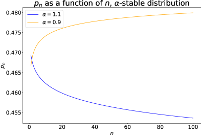
Figure 4: Evolution of $p_{n}$ when $X_{1}$ follows the $\alpha$-stable distribution. Here we considered $\varepsilon=0.1$. When $\alpha<1$, $p_{n}$ is increasing while it is decreasing, as expected, when $\alpha>1$.

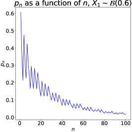
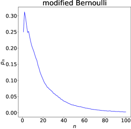
Figure 5: Left: evolution of $p_{n}$ when $X_{1}$ follows a Bernoulli distribution. Here we took $\varepsilon=0.1$. Right: same example, with some mass added at $\mu+\varepsilon$. We observe that the sequence $(p_{n})_{n\geq 1}$ is decreasing for sufficiently large $n$, as predicted by Theorem 6.

Appendix F Technical results

F.1 On the existence of $\tau$

For a subset $A$ of $\mathbb{R}^{D}$, we denote by $C(A)$ its convex hull, and by $\textup{int}(A)$ its interior.

Lemma 13 (Existence of $\tau$).

Let $X\in\mathbb{R}^{D}$ be a random variable with logaritmic moment generating function $\varphi$, support $\mathcal{S}$, and mean $\mu$. We assume that $X$ is absolutely continuous with respect to the Lebesgue measure, and that there exists $\alpha\in]0,\infty]$ such that $\{t\in\mathbb{R}^{D}|\varphi(t)<\infty\}=U_{\alpha}$, where $U_{\alpha}$ denotes the ball of radius $\alpha$. Let $\lambda_{\min}$ (resp. $\lambda_{\max}$) denote the minimal (resp. maximal) eigenvalue of $\nabla^{2}\varphi$. Then, for all $\varepsilon\in\mathbb{R}^{D}$ with strictly positive entries such that $\mu+\varepsilon\in\textup{int}(C(\mathcal{S}))$ and

$$\min_{1\leq i\leq D}\frac{\varepsilon_{i}}{\left\lVert\varepsilon\right\rVert}>\sqrt{2\left(1-\sqrt{\frac{\lambda_{\min}}{\lambda_{\max}}}\right)}\,,$$ (52)

there exists $\tau\in U_{\alpha}$ with strictly positive entries such that $\nabla\varphi(\tau)=\mu+\varepsilon$.

Remark 14.

Assumption (52) is quite restrictive. Indeed, assuming for a moment that $\left\lVert\varepsilon\right\rVert=1$, we see that the locus of points such that $\varepsilon_{i}>c$ for all $i$ is empty whenever $c\geq 1/\sqrt{d}$. Therefore, one needs

$$1-\frac{1}{2d}\leq\frac{\lambda_{\min}}{\lambda_{\max}}\left(\leq 1\right)$$

for Eq. (52) to hold for a non-empty set of points. For large $d$, this means requiring nearly isotropic $\nabla^{2}\varphi$.

Proof  Let $\varepsilon\in\mathbb{R}^{D}$ satisfying our assumptions. Since $\{t\in\mathbb{R}^{D}|\varphi(t)<\infty\}=U_{\alpha}$, $\varphi$ is “steep” in the sense of Barndorff-Nielsen (1978), and his Theorem 9.2 implies then that $\nabla\varphi(U_{\alpha})=\textup{int}(C(\mathcal{S}))$. Therefore, there exists $\tau\in U_{\alpha}$ such that $\nabla\varphi(\tau)=\mu+\varepsilon$.

All that is left to do is to show that all entries of $\tau$ are strictly positive. Since $\varphi$ is $\lambda_{\max}$-smooth, one can write

$$\frac{1}{\lambda_{\max}}\left\lVert\nabla\varphi(\tau)-\nabla\varphi(0)\right\rVert^{2}\leq(\nabla\varphi(\tau)-\nabla\varphi(0))^{\top}(\tau-0)=(\mu+\varepsilon-\mu)^{\top}\tau=\varepsilon^{\top}\tau\,.$$ (53)

Thus we have proved that $\varepsilon^{\top}\tau\geq\frac{1}{\lambda_{\max}}\left\lVert\varepsilon\right\rVert^{2}$. In particular, $\tau$ points in the same direction as $\varepsilon$. Though this is not sufficient to conclude: the halfspace of directing vector $\varepsilon$ contains points having non-positive coordinates. We note that, since $X$ is absolutely continuous, $\lambda_{\min}>0$, and $\varphi$ is $\lambda_{\min}$-strongly convex. Therefore,

$$(\nabla\varphi(\tau)-\nabla\varphi(0))^{\top}(\tau-0)\geq\lambda_{\min}\left\lVert\tau-0\right\rVert^{2}\,,$$ (54)

that is, $\varepsilon^{\top}\tau\geq\lambda_{\min}\left\lVert\tau\right\rVert^{2}$. Combining both bounds, we see that

$$\varepsilon^{\top}\tau\geq\sqrt{\frac{1}{\lambda_{\max}}\left\lVert\varepsilon\right\rVert^{2}\cdot\lambda_{\min}\left\lVert\tau\right\rVert^{2}}\,,$$

from which we deduce that

$$\cos(\varepsilon,\tau)\geq\sqrt{\frac{\lambda_{\min}}{\lambda_{\max}}}\,.$$ (55)

Equivalently, the angle between $\varepsilon$ and $\tau$ is less than $\theta_{0}\vcentcolon=\arccos\left(\sqrt{\frac{\lambda_{\min}}{\lambda_{\max}}}\right)$, meaning that $\tau$ belongs to $\mathcal{C}$ the half-cone of direction $\varepsilon$ and aperture $2\theta_{0}$.

Let us now prove that, under our assumption, no point of $\mathcal{C}$ has a negative coordinate. Without loss of generality, we can assume that $\left\lVert\varepsilon\right\rVert=\left\lVert\tau\right\rVert=1$. Using Eq. (55), we see that

$$\left\lVert\varepsilon-\tau\right\rVert^{2}=1+1-2\varepsilon^{\top}\tau\leq 2\left(1-\sqrt{\frac{\lambda_{\min}}{\lambda_{\max}}}\right)=\vcentcolon\rho^{2}\,.$$

To put it plainly, $\tau$ belongs to $\mathcal{B}$, the closed ball of center $\varepsilon$ and radius $\rho$. The distance from the center of $\mathcal{B}$ to each hyperplane $\{x_{i}=0\}$ is given by $\varepsilon_{i}$. Our assumption guarantees that $\varepsilon_{i}>\rho$ for all $i\in[d]$, thus $\mathcal{B}$ does not intersect any of the hyperplanes $\{x_{i}=0\}$. In particular, all point inside $\mathcal{B}$ have positive coordinates, and since $\tau\in\mathcal{B}$ we can conclude.  

Figure 6: Visual help for the proof of Lemma 13. The vector $\tau$ is contained in a half cone of axis $\varepsilon$ and angle $\theta_{0}$ (in red).

F.2 On the characteristic function of a random vector with non-zero density

In this section, we state and prove the following result, which is a straightforward multivariate extension of Lemma 3 in Chapter XV.7 of Feller (2008).

Lemma 15 (Characteristic function of random vector).

Let $X\in\mathbb{R}^{p}$ be a random vector with non-zero density almost everywhere. Then

$$\forall t\neq 0,\qquad\left\lvert\operatorname{\mathbb{E}}\left[\mathrm{exp}\left(\mathbf{i}\langle t,X\rangle\right)\right]\right\rvert<1\,.$$

Proof  Let us notice that the triangle inequality guarantees that $\left\lvert\operatorname{\mathbb{E}}\left[\mathrm{exp}\left(\mathbf{i}\langle t,X\rangle\right)\right]\right\rvert\leq 1$ for any $t\in\mathbb{R}^{p}$. Therefore, one only needs to show that $\left\lvert\operatorname{\mathbb{E}}\left[\mathrm{exp}\left(\mathbf{i}\langle t,X\rangle\right)\right]\right\rvert\neq 1$, which we will achieve reasoning by contradiction.

First, let us suppose that there exists $t\neq 0$ such that $\operatorname{\mathbb{E}}\left[\mathrm{exp}\left(\mathbf{i}\langle t,X\rangle\right)\right]=1$. Then the expectation of the non-negative function $x\mapsto 1-\cos\langle t,x\rangle$ is exactly $0$, meaning that $\langle t,x\rangle=0$ modulo $2\pi$ wherever $X$ has non-zero mass. Since $t\neq 0$, this implies that $X$ is supported in the collection of hyperplanes defined by

$$\langle t,x\rangle=2k\pi,\qquad k\in\mathbb{Z}\,,$$

which contradicts $X$ having non-zero density everywhere.

Let us now come back to the original problem, and assume that $\left\lvert\operatorname{\mathbb{E}}\left[\mathrm{exp}\left(\mathbf{i}\langle t,X\rangle\right)\right]\right\rvert=1$. Therefore there exists $b\in\mathbb{R}$ such that $\left\lvert\operatorname{\mathbb{E}}\left[\mathrm{exp}\left(\mathbf{i}\langle t,X\rangle\right)\right]\right\rvert=\operatorname{e}^{\mathbf{i}b}$. Since $t\neq 0$, there exists a vector $c\in\mathbb{R}^{p}$ such that $b=\langle t,c\rangle$, and one can write

$$\operatorname{\mathbb{E}}\left[\mathrm{exp}\left(\mathbf{i}\langle t,X-c\rangle\right)\right]=1\,.$$

We recognize the characteristic function of the random vector $Y\vcentcolon=X-c$, which also has non-zero density everywhere. Applying the previous reasoning to $Y$ also brings contradiction, and we can conclude.

References

- Althaus (2003) S. L. Althaus. Collective preferences in democratic politics: Opinion surveys and the will of the people. Cambridge University Press, 2003.
- Bach (2008) F. R. Bach. Bolasso: model consistent lasso estimation through the bootstrap. In Proceedings of the 25th international conference on Machine learning, pages 33–40, 2008.
- Bahadur and Ranga Rao (1960) R. R. Bahadur and R. Ranga Rao. On deviations of the sample mean. The Annals of Mathematical Statistics, 31(4):1015–1027, 1960.
- Baldi and Sadowski (2014) P. Baldi and P. Sadowski. The dropout learning algorithm. Artificial intelligence, 210:78–122, 2014.
- Barndorff-Nielsen (1978) O. E. Barndorff-Nielsen. Information and exponential families. Wiley, 1978.
- Barron (2019) J. T. Barron. A general and adaptive robust loss function. In Proceedings of the IEEE/CVF Conference on Computer Vision and Pattern Recognition, pages 4331–4339, 2019.
- Bartlett et al. (1998) P. Bartlett, Y. Freund, W. S. Lee, and R. E. Schapire. Boosting the margin: A new explanation for the effectiveness of voting methods. The annals of statistics, 26(5):1651–1686, 1998.
- Bartlett et al. (2006) P. L. Bartlett, M. I. Jordan, and J. D. McAuliffe. Convexity, classification, and risk bounds. Journal of the American Statistical Association, 101(473):138–156, 2006.
- Bates and Granger (1969) J. M. Bates and C. W. Granger. The combination of forecasts. Journal of the operational research society, 20(4):451–468, 1969.
- Berman et al. (2018) M. Berman, A. R. Triki, and M. B. Blaschko. The Lovász-softmax loss: A tractable surrogate for the optimization of the intersection-over-union measure in neural networks. In Proceedings of the IEEE conference on computer vision and pattern recognition, pages 4413–4421, 2018.
- Bickel and Doksum (2015) P. J. Bickel and K. A. Doksum. Mathematical statistics: basic ideas and selected topics, volume I (Second edition). Chapman and Hall/CRC, 2015.
- Biggs et al. (2022) F. Biggs, V. Zantedeschi, and B. Guedj. On margins and generalisation for voting classifiers. Advances in Neural Information Processing Systems, 35:9713–9726, 2022.
- Breiman (1996) L. Breiman. Bagging predictors. Machine Learning, 24(2):123–140, 1996.
- Breiman (2001) L. Breiman. Random forests. Machine learning, 45(1):5–32, 2001.
- Brown et al. (2001) L. D. Brown, T. T. Cai, and A. DasGupta. Interval estimation for a binomial proportion. Statistical science, 16(2):101–133, 2001.
- Bühlmann and Yu (2002) P. Bühlmann and B. Yu. Analyzing bagging. The annals of Statistics, 30(4):927–961, 2002.
- Burda et al. (2016) Y. Burda, R. Grosse, and R. Salakhutdinov. Importance weighted autoencoders. In International Conference on Learning Representations, 2016.
- Cannings and Samworth (2017) T. I. Cannings and R. J. Samworth. Random-projection ensemble classification. Journal of the Royal Statistical Society Series B: Statistical Methodology, 79(4):959–1035, 2017.
- Casa et al. (2021) A. Casa, L. Scrucca, and G. Menardi. Better than the best? answers via model ensemble in density-based clustering. Advances in Data Analysis and Classification, 15:599–623, 2021.
- Chu-Carroll et al. (2003) J. Chu-Carroll, K. Czuba, J. Prager, and A. Ittycheriah. In question answering, two heads are better than one. In Proceedings of the 2003 Human Language Technology Conference of the North American Chapter of the Association for Computational Linguistics, pages 24–31, 2003.
- Clemen (1989) R. T. Clemen. Combining forecasts: A review and annotated bibliography. International journal of forecasting, 5(4):559–583, 1989.
- Condorcet (1785) N. Condorcet. Essai sur l’application de l’analyse à la probabilité des décisions rendues à la pluralité des voix. Imprimerie Royale, 1785. Reprinted by Cambridge University Press in 2014.
- Dekel and Shamir (2009) O. Dekel and O. Shamir. Vox populi: Collecting high-quality labels from a crowd. In COLT, 2009.
- Diaconis (1988) P. Diaconis. Recent progress on de Finetti’s notions of exchangeability. Bayesian statistics, 3:111–125, 1988.
- Dougherty and Edward (2009) K. L. Dougherty and J. Edward. Odd or even: Assembly size and majority rule. The Journal of politics, 71(2):733–747, 2009.
- Feller (2008) W. Feller. An introduction to probability theory and its applications, vol. II. John Wiley & Sons, 2008.
- Freund and Schapire (1997) Y. Freund and R. E. Schapire. A decision-theoretic generalization of on-line learning and an application to boosting. Journal of computer and system sciences, 55(1):119–139, 1997.
- Friedman and Hall (2007) J. H. Friedman and P. Hall. On bagging and nonlinear estimation. Journal of statistical planning and inference, 137(3):669–683, 2007.
- Gal and Ghahramani (2016) Y. Gal and Z. Ghahramani. Dropout as a bayesian approximation: Representing model uncertainty in deep learning. In international conference on machine learning, pages 1050–1059. PMLR, 2016.
- Galton (1907) F. Galton. Vox populi. Nature, 75(1949):450–451, 1907.
- Genest and Zidek (1986) C. Genest and J. V. Zidek. Combining probability distributions: A critique and an annotated bibliography. Statistical Science, 1(1):114–135, 1986.
- George (1999) E. I. George. Bayesian model averaging: A tutorial: Comment. Statistical Science, 14(4):409–412, 1999.
- Germain et al. (2015) P. Germain, A. Lacasse, F. Laviolette, M. March, and J.-F. Roy. Risk bounds for the majority vote: From a PAC-Bayesian analysis to a learning algorithm. Journal of Machine Learning Research, 16(26):787–860, 2015.
- Gneiting and Raftery (2005) T. Gneiting and A. E. Raftery. Weather forecasting with ensemble methods. Science, 310(5746):248–249, 2005.
- Gneiting and Raftery (2007) T. Gneiting and A. E. Raftery. Strictly proper scoring rules, prediction, and estimation. Journal of the American statistical Association, 102(477):359–378, 2007.
- Grinsztajn et al. (2022) L. Grinsztajn, E. Oyallon, and G. Varoquaux. Why do tree-based models still outperform deep learning on typical tabular data? In Thirty-sixth Conference on Neural Information Processing Systems, Datasets and Benchmarks Track, 2022.
- Hall (1992) P. Hall. The bootstrap and Edgeworth expansion. Springer Science & Business Media, 1992.
- Hansen and Salamon (1990) L. K. Hansen and P. Salamon. Neural network ensembles. IEEE Transactions on Pattern Analysis and Machine Intelligence, 12(10):993–1001, 1990.
- Ho (1998) T. K. Ho. The random subspace method for constructing decision forests. IEEE transactions on pattern analysis and machine intelligence, 20(8):832–844, 1998.
- Hoeting et al. (1999) J. A. Hoeting, D. Madigan, A. E. Raftery, and C. T. Volinsky. Bayesian model averaging: a tutorial (with comments by m. clyde, david draper and ei george, and a rejoinder by the authors. Statistical science, 14(4):382–417, 1999.
- Hron et al. (2018) J. Hron, A. Matthews, and Z. Ghahramani. Variational bayesian dropout: pitfalls and fixes. In International conference on machine learning, pages 2019–2028. PMLR, 2018.
- Huber (1964) P. J. Huber. Robust estimation of a location parameter. Annals of Mathematical Statistics, 35:73–101, 1964.
- Joutard (2017) C. Joutard. Multidimensional strong large deviation results. Metrika, 80(6):663–683, 2017.
- Koriat (2012) A. Koriat. When are two heads better than one and why? Science, 336(6079):360–362, 2012.
- Krogh and Vedelsby (1994) A. Krogh and J. Vedelsby. Neural network ensembles, cross validation, and active learning. Advances in neural information processing systems, 7, 1994.
- Kuncheva (2014) L. I. Kuncheva. Combining pattern classifiers: methods and algorithms. John Wiley & Sons, 2014.
- Laan et al. (2017) A. Laan, G. Madirolas, and G. G. De Polavieja. Rescuing collective wisdom when the average group opinion is wrong. Frontiers in Robotics and AI, 4:56, 2017.
- Ladha (1993) K. K. Ladha. Condorcet’s jury theorem in light of de Finetti’s theorem: Majority-rule voting with correlated votes. Social Choice and Welfare, 10:69–85, 1993.
- Lakshminarayanan et al. (2017) B. Lakshminarayanan, A. Pritzel, and C. Blundell. Simple and scalable predictive uncertainty estimation using deep ensembles. Advances in neural information processing systems, 30, 2017.
- Lam and Suen (1997) L. Lam and S. Suen. Application of majority voting to pattern recognition: an analysis of its behavior and performance. IEEE Transactions on Systems, Man, and Cybernetics-Part A: Systems and Humans, 27(5):553–568, 1997.
- Larsen (2023) K. G. Larsen. Bagging is an optimal PAC learner. pages 450–458, 2023.
- Laurent et al. (2023) O. Laurent, A. Lafage, E. Tartaglione, G. Daniel, J.-m. Martinez, A. Bursuc, and G. Franchi. Packed ensembles for efficient uncertainty estimation. In International Conference on Learning Representations, 2023.
- Ma et al. (2020) X. Ma, H. Huang, Y. Wang, S. Romano, S. Erfani, and J. Bailey. Normalized loss functions for deep learning with noisy labels. In International conference on machine learning, pages 6543–6553. PMLR, 2020.
- Manski (2010) C. F. Manski. When consensus choice dominates individualism: Jensen’s inequality and collective decisions under uncertainty. Quantitative Economics, 1(1):187–202, 2010.
- Marshall and Proschan (1965) A. W. Marshall and F. Proschan. An inequality for convex functions involving majorization. Journal of Mathematical Analysis and Applications, 12(1):87–90, 1965.
- Marshall et al. (2011) A. W. Marshall, I. Olkin, and B. Arnold. Inequalities: Theory of Majorization and Its Applications. Springer, 2011.
- Masnadi-Shirazi and Vasconcelos (2008) H. Masnadi-Shirazi and N. Vasconcelos. On the design of loss functions for classification: theory, robustness to outliers, and savageboost. Advances in neural information processing systems, 21, 2008.
- Masnadi-Shirazi et al. (2010) H. Masnadi-Shirazi, V. Mahadevan, and N. Vasconcelos. On the design of robust classifiers for computer vision. In 2010 IEEE Computer Society Conference on Computer Vision and Pattern Recognition, pages 779–786. IEEE, 2010.
- Mason et al. (1999) L. Mason, J. Baxter, P. Bartlett, and M. Frean. Boosting algorithms as gradient descent. Advances in neural information processing systems, 12, 1999.
- Mattei and Frellsen (2022) P.-A. Mattei and J. Frellsen. Uphill roads to variational tightness: Monotonicity and Monte Carlo objectives. arXiv preprint arXiv:2201.10989, 2022.
- McCullagh (2018) P. McCullagh. Tensor methods in statistics (Second edition). Dover Books on Mathematics, 2018.
- McNees (1992) S. K. McNees. The uses and abuses of ‘consensus’ forecasts. Journal of Forecasting, 11(8):703–710, 1992.
- Nikodem (2014) K. Nikodem. On strongly convex functions and related classes of functions. In Handbook of functional equations, pages 365–405. Springer, 2014.
- Noh et al. (2017) H. Noh, T. You, J. Mun, and B. Han. Regularizing deep neural networks by noise: Its interpretation and optimization. Advances in Neural Information Processing Systems, 30, 2017.
- Parmigiani and Inoue (2009) G. Parmigiani and L. Inoue. Decision theory: Principles and approaches. John Wiley & Sons, 2009.
- Perrone (1993) M. P. Perrone. Improving regression estimation: Averaging methods for variance reduction with extensions to general convex measure optimization. PhD thesis, Brown University, 1993.
- Petrov (1965) V. V. Petrov. On the probabilities of large deviations for sums of independent random variables. Theory of Probability & Its Applications, 10(2):287–298, 1965.
- Prelec et al. (2017) D. Prelec, H. S. Seung, and J. McCoy. A solution to the single-question crowd wisdom problem. Nature, 541(7638):532–535, 2017.
- Probst and Boulesteix (2018) P. Probst and A.-L. Boulesteix. To tune or not to tune the number of trees in random forest. Journal of Machine Learning Research, 18:1–18, 2018.
- Rasmussen and Williams (2006) C. E. Rasmussen and C. K. Williams. Gaussian processes for machine learning, volume 1. Springer, 2006.
- Riesselman et al. (2018) A. J. Riesselman, J. B. Ingraham, and D. S. Marks. Deep generative models of genetic variation capture the effects of mutations. Nature methods, 15(10):816–822, 2018.
- Rokach (2010) L. Rokach. Ensemble-based classifiers. Artificial intelligence review, 33:1–39, 2010.
- Russell et al. (2015) N. Russell, T. B. Murphy, and A. E. Raftery. Bayesian model averaging in model-based clustering and density estimation. arXiv preprint arXiv:1506.09035, 2015.
- Scornet et al. (2015) E. Scornet, G. Biau, and J.-P. Vert. Consistency of random forests. The Annals of Statistics, 43(4):1716–1741, 2015.
- Serre (2010) D. Serre. Matrices. Theory and Applications (Second edition). Springer, 2010.
- Shalev-Shwartz and Ben-David (2014) S. Shalev-Shwartz and S. Ben-David. Understanding machine learning: From theory to algorithms. Cambridge university press, 2014.
- Shteingart et al. (2020) H. Shteingart, E. Marom, I. Itkin, G. Shabat, M. Kolomenkin, M. Salhov, and L. Katzir. Majority voting and the condorcet’s jury theorem. arXiv preprint arXiv:2002.03153, 2020.
- Simoiu et al. (2019) C. Simoiu, C. Sumanth, A. Mysore, and S. Goel. Studying the “wisdom of crowds” at scale. In Proceedings of the AAAI Conference on Human Computation and Crowdsourcing, volume 7, pages 171–179, 2019.
- Small (2010) C. G. Small. Expansions and asymptotics for statistics. Chapman and Hall/CRC, 2010.
- Srivastava et al. (2014) N. Srivastava, G. Hinton, A. Krizhevsky, I. Sutskever, and R. Salakhutdinov. Dropout: a simple way to prevent neural networks from overfitting. The journal of machine learning research, 15(1):1929–1958, 2014.
- Stone (1961) M. Stone. The opinion pool. The Annals of Mathematical Statistics, pages 1339–1342, 1961.
- Struski et al. (2022) Ł. Struski, M. Mazur, P. Batorski, P. Spurek, and J. Tabor. Bounding evidence and estimating log-likelihood in vae. arXiv preprint arXiv:2206.09453, 2022.
- Sun et al. (2022) R. Sun, A. Ramé, C. Masson, N. Thome, and M. Cord. Towards efficient feature sharing in mimo architectures. In Proceedings of the IEEE/CVF Conference on Computer Vision and Pattern Recognition, pages 2697–2701, 2022.
- Surowiecki (2005) J. Surowiecki. The wisdom of crowds. Anchor, 2005.
- Tschandl et al. (2018) P. Tschandl, C. Rosendahl, and H. Kittler. The HAM10000 dataset, a large collection of multi-source dermatoscopic images of common pigmented skin lesions. Scientific data, 5(1):1–9, 2018.
- Viering and Loog (2023) T. Viering and M. Loog. The shape of learning curves: A review. IEEE Transactions on Pattern Analysis and Machine Intelligence, 45(6):7799–7819, 2023.
- Viering et al. (2019) T. Viering, A. Mey, and M. Loog. Open problem: Monotonicity of learning. In Conference on Learning Theory, pages 3198–3201. PMLR, 2019.
- Yang et al. (2023) J. Yang, R. Shi, D. Wei, Z. Liu, L. Zhao, B. Ke, H. Pfister, and B. Ni. MedMNIST v2-A large-scale lightweight benchmark for 2D and 3D biomedical image classification. Scientific Data, 10(1):41, 2023.