FisherRF: Active View Selection and Uncertainty Quantification for Radiance Fields using Fisher Information

Abstract

This study addresses the challenging problem of active view selection and uncertainty quantification within the domain of Radiance Fields. Neural Radiance Fields (NeRF) have greatly advanced image rendering and reconstruction, but the limited availability of 2D images poses uncertainties stemming from occlusions, depth ambiguities, and imaging errors. Efficiently selecting informative views becomes crucial, and quantifying NeRF model uncertainty presents intricate challenges. Existing approaches either depend on model architecture or are based on assumptions regarding density distributions that are not generally applicable. By leveraging Fisher Information, we efficiently quantify observed information within Radiance Fields without ground truth data. This can be used for the next best view selection and pixel-wise uncertainty quantification. Our method overcomes existing limitations on model architecture and effectiveness, achieving state-of-the-art results in both view selection and uncertainty quantification, demonstrating its potential to advance the field of Radiance Fields. Our method with the 3D Gaussian Splatting backend could perform view selections at 70 fps. Source code and other materials are available at https://jiangwenpl.github.io/FisherRF/.

1 Introduction

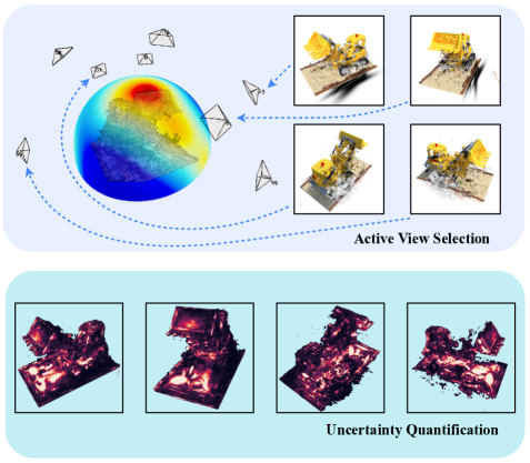
Figure 1: A brief overview of our method Given a radiance field that was trained with a limited number of views, our method could find the next best view that could maximize information gain by computing the Fisher Information of the radiance field. We illustrate the information gain as a heat map on the viewing sphere and show four of the candidate views. Our model can quantify pixel-wise uncertainty, visualized on the bottom, by examining the Fisher Information on the related parameters of the ray.

Neural Radiance Fields brought back image rendering and reconstruction from multiple views to the center of attention in the field of computer vision. Novel volumetric representations of radiance fields and differentiable volumetric rendering enabled unprecedented advances in image-based rendering of complex scenes both in terms of perceptual quality and speed. Recently, 3D Gaussian Splatting has demonstrated distinct advantages in real-time rendering and explicit point-based parameterizations without neural representations. However, the majority of approaches that estimate a radiance field need tens of viewpoints. When we are limited to a low number of 2D images, uncertainty naturally arises from occlusions, depth ambiguities, and aleatoric errors in the imaging process. It is crucial to establish a criterion for selecting information-maximizing views before knowing what the actual error will be in these views. Quantifying the observed information of a NeRF model is challenging, given that NeRF models are typically regression-based and scene-specific. The challenge intensifies when we aim to leverage quantified uncertainties for active view selection, especially when the selection candidates are only $SE(3)$ camera poses for acquiring new observations, a.k.a capturing new images.

Previous approaches for uncertainty quantification and view selection can be broadly categorized into two groups: variational white-box models and predictive black-box models. White-box models integrate conventional NeRF architectures with Bayesian models, such as reparameterization [25, 21, 26] and Normalizing Flows [32]. Black-box methods, on the other hand, do not modify the existing model architecture but seek to quantify predictive uncertainty by examining the distribution of predicted outcomes [40, 5].

White-box models depend on specific model architectures and are often characterized by slower training times due to the challenges associated with probabilistic learning. Conversely, existing black-box models either focus solely on studying the distribution of densities along a ray, assuming that the density distribution on a ray should be as sharp as possible, or rely on Monte Carlo-style sampling techniques [38] to quantify the perturbations of their model. In this study, our primary objective is to quantify the observed information of a Radiance Field model and utilize it to select the optimal view with the highest information gain. To achieve this, we propose the use of Fisher Information, which represents the expectation of observation information. This quantity is directly linked to the second-order derivatives or Hessian matrix of the loss function involved in optimizing Radiance Field models.

Importantly, the Hessian of the objective function in volumetric rendering is independent of ground truth data or the actual image measurement. This property allows us to compute the information gain between the training dataset and the candidate viewpoint pool using only the camera parameters of the candidate views. This capability facilitates an efficient next-best-view selection.

In addition to the information gain framework, the Hessian of the loss function has an intuitive interpretation: the perturbation at flat minima of the loss function. From an intuitive standpoint, one can perceive the Fisher Information matrix as a metric of the curvature of the log-likelihood function at specific parameter instantiations denoted as ${\bf w}^{*}$. Lower Fisher Information suggests that the log-likelihood function exhibits a flatter profile around ${\bf w}^{*}$, implying that the loss is less prone to changes when ${\bf w}^{*}$ is perturbed. The flat minimum interpretation has attracted substantial attention and research within various domains of machine learning [10, 14, 11, 33, 19]. Our method can be applied to any model that parametrizes explicitly the density and the radiance needed in volumetric rendering such as 3D Gaussian Splatting [13] and Plenoxels [29]. This allows us to derive pixel-wise uncertainty in the model’s predictions by examining the Fisher Information on parameters that contributed to the prediction for each pixel.

We implemented the computation of Fisher Information on top of two types of Radiance Field models: point-based 3D Gaussian Splatting [13] and Plenoxels [29]. In 3D Gaussians, we compute the Hessians of the mean, covariances, opacity, and spherical harmonics with respect to the negative log-likelihood. In Plenoxels, we compute the Hessians of density and spherical harmonics on the sparse voxel grid representation of Plenoxel with respect to its negative log-likelihood. When selecting candidates, we apply a greedy policy, choosing the view with the highest information gain. To make the computation of information gain tractable, we use an approximation of the decrease in entropy by its upper bound, which is the trace of the product of the Hessian of the candidate view times the Hessian with respect to all previous views. These matrices are highly sparse due to the disentangling of scene parameters with respect to disparate rays. The sparsity allows us a computation of the matrix trace above that is as cost-effective as back-propagation, enabling us to evaluate views at 70 fps when we use 3D Gaussian Splatting. We carried out an extensive evaluation in both active view selection and uncertainty quantification. Our evaluation contains the PSNR in the hold-out test as a function of the number of views and the selection regime (one or more views at a time) as well as an AUSE evaluation of the uncertainty and an evaluation of the stratification error. The quantitative and qualitative results unequivocally demonstrate that our approach surpasses previous methods and heuristic baseline by a significant margin. To summarize, our main contributions are as follows:

• A novel quantification of uncertainty that we use in computing the information gain of candidate views.

• An efficient computation of the information gain exploiting the sparse structure of the scene rendering problem.

• We were able to compute a pixel-wise uncertainty quantification and visualization.

• Extensive experimental evaluation showing that our active view selection outperforms existing active approaches.

2 Related Works

Active Learning and Radiance Fields are prosperous research fields with various research directions. In this section, we limit our literature overview on works on view selection and uncertainty quantification for radiance fields. We refer the readers to literature reviews if they are interested in Radiance Fields [8, 7] or Deep Active Learning [28, 41]. Besides, Fisher Information has been extensively studied in deep active learning [2, 1, 17, 16]. Notably, Kirsch et al. [14] unified existing works in active learning for deep learning problems from the perspective of Fisher Information, which shares many insights with our method.

Uncertainty Quantifications for Radiance Fields

In the Neural Radiance Fields, Chen et al. [5], Yan et al. [37] and Zhan et al. [40] attempted to quantify the uncertainty in a scene by the distribution of densities on a casted ray. Pan et al. [25] and Shen et al. [32, 31] designed Bayesian models by re-parametrizing the NeRF model. However, they only tackled the predictive uncertainty of the model that did not relate to the observed information of the parameters. Sunderhauf et al. [35] propose an additional uncertainty measure in uncharted regions, determined by the ray termination probability on the learned geometry. Regarding concurrent work, Goli et al. [9] also introduces Fisher information to quantify the uncertainty. However, they applied a considerable simplification by computing the Hessian over a hypothetical perturbation field, while we directly estimate the Fisher Information on the model parameters. Besides, the focus of their method is cleaning up noisy 3D positions in a NeRF model. Yan et al. [38] discussed the intuition of flat minimum and quantified the predictive uncertainty of neural mapping models through the lens of loss landscape. However, they only approximate the uncertainty of the variances from the output of neighboring points. Our method directly quantifies the observed information of the parameters by computing the Hessian matrix of the log-likelihood function of the model’s objective. To the best of our knowledge, we are the first method that quantifies the uncertainty of explicit radiance field models, thanks to the powerful framework of 3D Gaussian and our efficient formulation.

Active Learning for Radiance Field

Although the next best views selection problem was extensively studied before radiance fields gained popularity, there has not been much literature on active “training” view selection for novel view rendering. ActiveNeRF [25] studied the next best view selection and it is the closest approach to the view selection problem we are working on. Although Ran et al. [26], Yan et al. [38], Zhan [40] included the next best view selection in their neural mapping or reconstruction system, their goal was not to quantify the observed information of a radiance field.

3 Technical Approach

In this section, we first introduce the background knowledge of volumetric rendering in Sec. 3.1, which radiance field models, including our backbone model 3D Gaussian Splatting and Plenoxel, are widely used. We then introduce how we use Fisher Information in Sec. 3.2. By leveraging Fisher Information, we demonstrate how to select the next best view and next best batch of views in Sec. 3.3 and Sec. 3.4. Finally, we showcase that our method could quantify the pixel-wise uncertainties in Sec. 3.5.

3.1 Preliminaries: Volumetric Rendering and Gaussian Splatting

3D Gaussian Splatting [13], Plenoxels [29], and Neural Radiance Fields [22] all use volumetric rendering for image formation. Consider a camera ray $\text{r}(t)=\text{o}+t\text{d}$ originating from the camera center $\text{o}\in\mathcal{R}^{3}$ and passing through a specific pixel on the image plane. The color of the pixel can be expressed as:

$$C(\text{r})=\int_{t_{n}}^{t_{f}}T(t)\sigma(\text{r}(t))\text{c}(\text{r}(t),\text{d})\,dt\,$$ (1)

where $T(t)=\text{exp}\left(-\int_{t_{n}}^{t}\sigma(\text{r}(s))\,ds\right)$ denotes the accumulated transmittance, and $t_{n}$ and $t_{f}$ represent the near and far bounds within the scene. In practice, NeRF approximates the integral using stratified sampling and formulates it as a linear combination of sampled points:

$$\hat{C}(\text{r})=\sum_{i=1}^{N_{s}}T_{i}\left(1-\exp(-\sigma_{i}\delta_{i})\right){\bf c}_{i}$$ (2)

$$\alpha_{i}=\text{exp}\left(-\sum_{j=1}^{i-1}\sigma_{j}\delta_{j}\right)(1-\text{exp}(-\sigma_{i}\delta_{i}))$$ (3)

Here, $\delta_{i}=t_{i+1}-t_{i}$ represents the distance between adjacent samples, and $N_{s}$ indicates the number of samples. Based on this approach, NeRF approaches optimize the continuous function $F_{\theta}$ by minimizing the squared reconstruction errors between the ground truth obtained from RGB images ${\mathcal{I}_{i=1}^{N}}$ and the rendered pixel colors. Although 3D Gaussian Splatting has a different rendering pipeline, the image formation is still similar, whereas, in 3D Gaussian Splatting, ${\bf c}_{i}$ is the color of each 3D Gaussian given the view direction ${\bf d}$ and $\sigma_{i}$ is given by evaluating a 2D Gaussian with covariance $\Sigma$.

3.2 Fisher Information in Volumetric Rendering

Fisher Information is a measurement of information that an observation $({\bf x},{\bf y})$ carries about the unknown parameters $w$ that model $p({\bf y}|{\bf x};{\bf w})$. In the problem of novel view synthesis, $({\bf x},{\bf y})$ are the camera pose ${\bf x}$ and image observation ${\bf y}$ at pose ${\bf x}$, respectively, whereas ${\bf w}$ are the volumetric parameters of the radiance field. The objective of neural rendering is equivalent to minimizing the negative log likelihood (NLL) between rendered images and ground truth images on the holdout set, which inherently represents the quality of scene reconstruction

$$-\log p({\bf y}|{\bf x},{\bf w})=\left({\bf y}-f({\bf x},{\bf w})\right)^{T}\left({\bf y}-f({\bf x},{\bf w})\right)$$ (4)

where $f({\bf x},{\bf w})$ is our rendering model. Under regularity conditions [30], the Fisher Information of the model $\log p({\bf y}|{\bf x};{\bf w})$ is the Hessian of the log-likelihood function with respect to the model parameters ${\bf w}$:

$$\mathcal{I}({\bf w})=-\mathbb{E}_{{\bf y}|{\bf x}\sim p_{\bf w}}\big{[}\frac{\partial^{2}\log p({\bf y}|{\bf x},{\bf w})}{\partial{\bf w}^{2}}\big{|}{\bf w}\big{]}={\mathbf{H}}^{\prime\prime}[{\bf y}|{\bf x},{\bf w}]$$ (5)

where ${\mathbf{H}}^{\prime\prime}[{\bf y}|{\bf x},{\bf w}]$ is the Hessian matrix of Eq. (4).

3.3 Next Best View Selection Using Fisher Information

In the active view selection problem, we start with a training set $D^{train}$ and have an initial estimation of parameters ${\bf w}^{*}$ using $D^{train}$. The aim is to select the next best view that maximizes the Information Gain [18, 12, 15] between candidates views ${\bf x}^{acq}_{i}\in D^{pool}$ and $D^{train}$, where $D^{pool}$ is the pool of candidate views:

$$\mathcal{I}[{\bf w}^{*};\{{\bf y}^{acq}_{i}\}|\{{\bf x}^{acq}_{i}\},D^{train}]$$

$$=H[{\bf w}^{*}|D^{train}]-H[{\bf w}^{*}|\{{\bf y}^{acq}_{i}\},\{{\bf x}^{acq}_{i}\},D^{train}]$$ (6)

where $H[\cdot]$ is the entropy [14].

When the log-likelihood has the form of Eq. (4), in our case the rendering error, the difference of the entropies in the R.H.S. of Eq. (6) can be approximated as [14]:

$$\frac{1}{2}\log\det\left({\mathbf{H}}^{\prime\prime}[\{{\bf y}^{acq}_{i}\}|\{{\bf x}^{acq}_{i}\},{\bf w}^{*}]\;{\mathbf{H}}^{\prime\prime}[{\bf w}^{*}|D^{train}]^{-1}+I\right)$$

$$\leq\frac{1}{2}\operatorname{tr}\left({\mathbf{H}}^{\prime\prime}[\{{\bf y}^{acq}_{i}\}|\{{\bf x}^{acq}_{i}\},{\bf w}^{*}]\;{\mathbf{H}}^{\prime\prime}[{\bf w}^{*}|D^{train}]^{-1}\right).$$ (7)

As Fisher Information is additive, ${\mathbf{H}}^{\prime\prime}[{\bf w}^{*}|D^{train}]^{-1}$ can be computed by summing the Hessians of model parameters across all different views in $\{D_{train}\}$ before inverting. We can choose the next best view ${\bf x}^{acq}_{i}$ by optimizing

$$\operatorname*{arg\,max}_{{\bf x}^{acq}_{i}}\operatorname{tr}\left({\mathbf{H}}^{\prime\prime}[{\bf y}^{acq}_{i}|{\bf x}^{acq}_{i},{\bf w}^{*}]\;{\mathbf{H}}^{\prime\prime}[{\bf w}^{*}|D^{train}]^{-1}\right).$$ (8)

The Hessian ${\mathbf{H}}^{\prime\prime}[{\bf y}|{\bf x},{\bf w}^{*}]$ of our model can be computed as:

$${\mathbf{H}}^{\prime\prime}[{\bf y}|{\bf x},{\bf w}^{*}]=\nabla_{\bf w}f({\bf x};{\bf w}^{*})^{T}\nabla_{f({\bf x};{\bf w}^{*})}^{2}H[{\bf y}|f({\bf x};{\bf w}^{*})]\nabla_{\bf w}f({\bf x};{\bf w}^{*})$$ (9)

where ${\mathbf{H}}^{\prime\prime}[{\bf y}|{\bf x},{\bf w}^{*}]$ in our case is equal to the covariance of the RGB measurement that we set equal to one. Hence, the Hessian matrix can be computed just from the Jacobian matrix of $f({\bf x},{\bf w})$

$${\mathbf{H}}^{\prime\prime}[{\bf y}|{\bf x},{\bf w}^{*}]=\nabla_{\bf w}f({\bf x};{\bf w}^{*})^{T}\nabla_{\bf w}f({\bf x};{\bf w}^{*}).$$ (10)

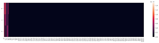
Figure 2: An example of the Jacobinas of the rendering equation on a casted ray. We plot the absolute values of the Jacobian of three channels in one ray w.r.t the sampled points on the ray in Plenoxel. Most sampled points in volumetric rendering only have very small values in their corresponding Jacobian matrix, prompting the sparsity of the Hessian matrix in Radiance Fields.

We can optimize the objective in Eq. (8) without knowing the ground truth of candidate views $\{{\bf y}^{acq}_{i}\}$, which was expected since the Fisher Information never depends on the observations themselves. The Hessian in (10) has only a limited number of off-diagonal elements because each pixel is considered independent in $-\log p({\bf y}|{\bf x},{\bf w})$. Furthermore, recent NeRF models [29, 24, 27, 34] typically employ structured local parameters that each parameter only contributes to the radiance and density of a limited spatial region for faster convergence and rendering. Therefore, only parameters that contribute to the color of the pixels would share non-zero values in the Hessian matrix ${\mathbf{H}}^{\prime\prime}[{\bf y}|{\bf x},{\bf w}^{*}]$. However, the number of optimizable parameters is typically more than 200 million, which means it is impossible to compute without sparsification or approximation. In practice, we apply Laplace approximation [6, 20] that approximates the Hessian matrix with its diagonal values plus a log-prior regularizer $\lambda I$

$${\mathbf{H}}^{\prime\prime}[{\bf y}|{\bf x},{\bf w}^{*}]\simeq\operatorname{diag}(\nabla_{\bf w}f({\bf x},{\bf w}^{*})^{T}\nabla_{\bf w}f({\bf x},{\bf w}^{*}))+\lambda I.$$ (11)

This approximation also allows us to invert the Hessian matrix ${\mathbf{H}}^{\prime\prime}[{\bf y}|{\bf x},{\bf w}^{*}]$ easily. We further showcase the sparsity of the Jacobian and Hessian matrix in Fig. 2 and Fig. 3.

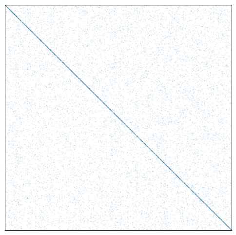
Figure 3: An example of the Hessian matrix on the parameters of Plenoxel. We compute the Hessian of the NLL function of volumetric rendering following the Eq. (10).

3.4 Batch Active View Selection

Selecting multiple views to capture new images is useful for its possible applications, such as view planning and scene reconstruction. If we directly use Eq. (8) to select a batch of acquisition samples $\{{\bf x}^{acq}_{i}\}$, we could possibly select very similar views inside the acquisition set $\{{\bf x}^{acq}_{i}\}$ as we do not consider the mutual information between our selections. However, we would face a combinatorial explosion if we directly attempt to maximize the expected information gain between training and acquisition samples and simultaneously minimize the mutual information across acquisition samples. Therefore, we employ a greedy optimization algorithm as illustrated in Alg. 1, which is $\nicefrac{{1}}{{e}}$-approximate in Fisher Information. When batch size $B$ is 1, our algorithm is equivalent to Eq. (8). Please note that we focus on batch active view selection instead of dataset subsampling as it is more related to real-world scenarios where we wish to plan a trajectory for an agent to acquire more training views.

Input: $\{{\mathbf{H}}^{\prime\prime}[{\bf w}^{*}|{\bf x}^{acq}_{i}]\}$, ${\mathbf{H}}^{\prime\prime}[{\bf w}^{*}|D^{train}]$, number of views to select $B$

Output: Selected Views $S_{B}$

1

2$S_{0}\leftarrow\emptyset$ ;

3 $H_{0}\leftarrow{\mathbf{H}}^{\prime\prime}[{\bf w}^{*}|D^{train}]$;

4

5for  $b\leftarrow 1$ to $B$ do

6       $i\leftarrow\operatorname*{arg\,max}_{{\bf x}^{acq}_{i}\in D^{pool}]\setminus S_{b-1}}\operatorname{tr}\left({\mathbf{H}}^{\prime\prime}[{\bf y}^{acq}_{i}|{\bf x}^{acq}_{i},{\bf w}^{*}]\;H_{b-1}^{-1}\right)$;

7       $S_{b}\leftarrow S_{b-1}\cup\{i\}$ ;

8       $H_{b}\leftarrow H_{b-1}+{\mathbf{H}}^{\prime\prime}[{\bf y}^{acq}_{i}|{\bf x}^{acq}_{i},{\bf w}^{*}]$ ;

9      

10 end for

Algorithm 1 Batch Active Views Selection

3.5 Pixel-wise Uncertainty with Volumetric Rendering

Previously, we discussed quantifying the uncertainty for any camera views. Our model can also be extended to obtain pixel-wise uncertainties. As we have discussed in Sec. 3.3, we can approximate the uncertainty on each parameter with the diagonal elements of the hessian matrix ${\mathbf{H}}^{\prime\prime}[{\bf y}^{acq}_{i}|{\bf x}^{acq}_{i},{\bf w}^{*}]$. In recent neural rendering models [13, 29], the parameters directly correspond to a spatial location in the scene. Therefore, we can compute the uncertainty in our rendered pixels by examining the diagonal Hessians along the casted ray for volumetric rendering

$$\mathbf{U}(\text{r})=\sum_{n=1}^{N_{s}}T_{i}\left(1-\exp(-\sigma_{n}\delta_{n})\right)tr({\bf G}_{n})$$ (12)

where ${\bf G}_{n}$ is the submatrix of ${\mathbf{H}}^{\prime\prime}[{\bf w}^{*}|D^{train}]$ containing the rows and columns that correspond to parameters at location $n$. Please note this is a relative uncertainty on the rendered pixels that treat each location equally. If we wish to estimate absolute uncertainties on predictions like depth maps, we need to denormalize the uncertainty in each term by its depth $d_{n}$.

4 Experiments

In this Section, we present the empirical evaluation of our approach. First, we introduce the details of our implementation in (Subsection 4.1). Then, we focus on the experiments of active view selection and compare our method quantitatively and qualitatively against the previous method. Finally, we present more results of our method on uncertainty quantification. results (Subsection 4.3).

4.1 Implementation Details

Our method can be applied to various kinds of neural rendering models. We implement the computation of Fisher Information on Plenoxels [29] and 3D Gaussian Splatting [13] with customized CUDA kernels.

As shown in Eq. 10, the diagonal Hessian matrixes can be implemented as efficiently as a back-propagation. Therefore, our customized CUDA kernel that computes diagonal Hessians for 3D Gaussian Splatting achieved more than 70 fps on a Nvidia RTX3090 GPU. The log-prior regularizer $\lambda$ in Eq. 11 is $10^{-6}$ across all experiments. The supplementary materials and code release will present other hyper-parameters and implementation details.

4.2 Active View Selection

We conducted extensive experiments on view selections to demonstrate that our expected information gain could help the model find the next best views. Here, we first introduce the dataset we use and detailed experimental settings. Then, we compare our method with random baselines and previous state-of-the-art [25] quantitatively and qualitatively.

Datasets

Our approach is extensively evaluated on two common benchmark datasets: Blender Dataset [22] and the challenging real-world Mip-NeRF360 dataset [3]. The Blender dataset comprises eight synthetic objects with intricate geometry and realistic non-Lambertian materials. Each scene in this dataset includes 100 training and 200 test views, all with a resolution of $800\times 800$. Our method uses the 100 training views as a candidate pool to select training views, and we evaluate all the models on the full 200 views test set. We use the default training configuration as in 3D Gaussian and Plenoxels for this dataset. Mip-NeRF360 [3] is a real-world $360^{\circ}$ dataset captured for nine different scenes. It has been widely used as a quality benchmark for novel view synthesis models [4, 23]. We train our models at the resolution of $1066\times 1600$ following 3D Gaussian Splatting [13].

Metrics

Our evaluations utilize image quality metrics such as peak signal-to-noise ratio (PSNR) and structural similarity index (SSIM) [36]. Additionally, we incorporate LPIPS [42], which provides a more accurate reflection of human perception.

Baselines

We quantitatively and qualitatively compare our method against the current state-the-art ActiveNeRF [25] and random selection baseline. To make a fair comparison with ActiveNeRF [25], we re-implemented a similar variance estimation algorithm in 3D Gaussian Splatting and Plenoxel in CUDA. We assign each 3D Gaussian (or grid cell in Plenoxels) a variance parameter and use volumetric rendering to render a variance map. More details about our re-implementation can be found in the supplementary materials.

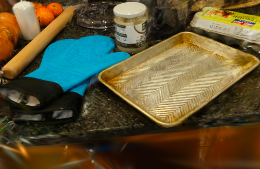
Figure 4: Qualitative Study of our method on Mip360 Dataset From the top to bottom are results from ActiveNeRF, random baseline, our method, and the ground truth. All the models in this figure are implemented on top of 3D Gaussian Splatting [13] for better performance on this challenging dataset. We could see baseline models exhibited artifacts in some renderings due to their lack of constraints from nearby training views.

PSNR/SSIM	400 Steps	8000 Steps	350k Steps

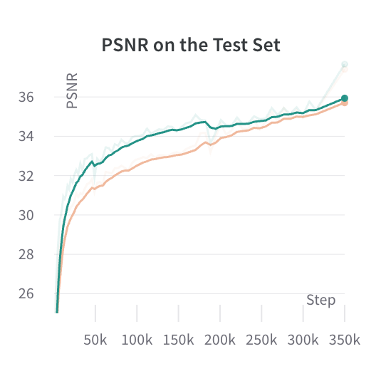
Figure 5: A comparative study on the effects of the number of training views and view selection strategies. The top renderings are from the random baseline, and the bottom are from our method. Both are implemented with 3D Gaussian Splatting. We further extend our experiments on the Blender dataset from selecting 20 views to selecting 80 views. We continue training over the model by selecting one new view every 100 epochs. Although the effects of view selection vanish after the model is trained with a sufficient number of views, our method is still better than the random baseline as it was less impacted by the degeneration and local minima when the model was only trained with a limited number of views at the early stage.

ActiveNeRF	Random	Ours

Figure 6: Qualitative Results on Blender Dataset with 20 Training Views All the methods are implemented on 3D Gaussian Splatting and compared in the same condition except for different training views selected by different methods. As can be seen, ActiveNeRF suffered from significant artifacts at a large scale, and the random baseline also experienced blurry details when zooming in. Our method, however, could select the training views that are most necessary for the current model, thus preventing catastrophic degeneration.

ActiveNeRF	Random	Ours

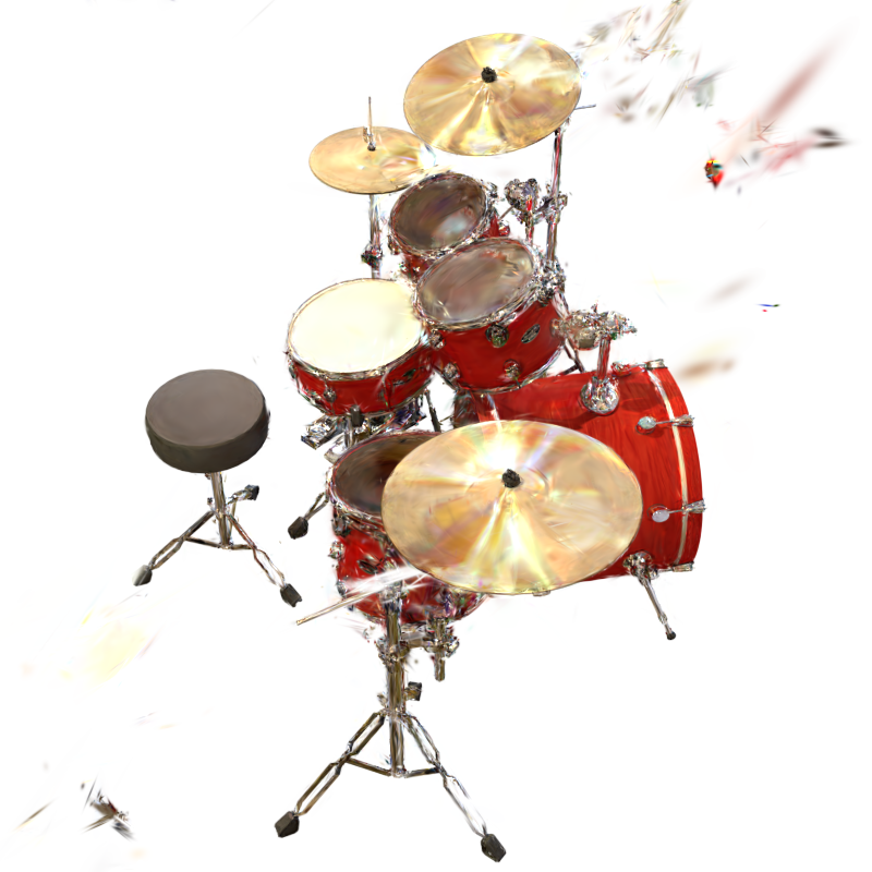
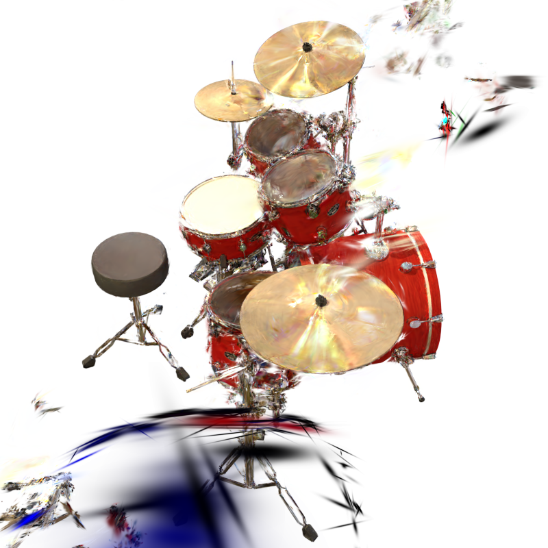
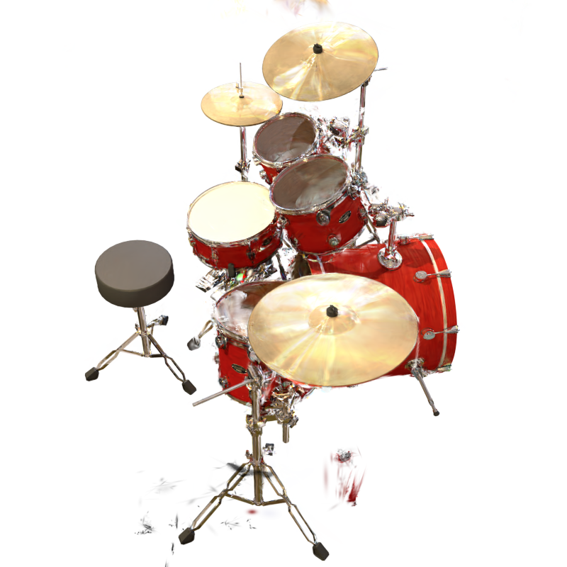
Figure 7: Qualitative Results on Blender Dataset with 10 Training Views We also qualitatively compare the method with ActiveNeRF and random baseline implemented on top of 3D Gaussian Splatting. By selecting the training views with maximum information gain, our model could still help the 3D Gaussian Splatting to get impressive views under this challenging setting.

Experiment Settings

We experiment with our model with 3D Gaussian Splatting backend on both the next view selection and the next batch of view selections across both the Blender and Mip360 Dataset. Each model is initialized with the same random seed and was trained on the same four uniform views. Each model is trained for 30,000 iterations following the default configurations of 3D Gaussian Splatting [13]. Similar to the training program of Gaussian Splatting, we reset the opacity every time we select new views to avoid degeneration of the training procedure. All the external settings in the experiment are kept the same except for the view selection algorithms.

Similarly, we also showcase the implementations of our active view selection algorithm on Plenoxels in the Blender Dataset. The experimental settings for initial views and view selection schedules are the same, except view selection was made every four epochs.

• Sequential Active View Selection: 1 new view is selected every 100 epochs till the model has 20 training views.

• Batch Active View Selection: 4 new views are selected every 300 epochs till the model has 20 training views.

Method	PSNR $\uparrow$	SSIM $\uparrow$	LPIPS $\downarrow$
ActiveNeRF*	26.240	0.8560	0.1240
Plenoxel + Random	23.242	0.8617	0.1582
Plenoxel + ActiveNeRF	23.522	0.8573	0.1499
Plenoxel + ActiveNeRF†)	23.147	0.8571	0.1478
3D Gaussian + Random	28.732	0.9389	0.0534
3D Gaussian + Random†	27.135	0.9267	0.0651
3D Gaussian + ActiveNeRF	25.854	0.9157	0.0766
3D Gaussian + ActiveNeRF†	27.326	0.9116	0.0756
Plenoxel + Ours	24.513	0.8759	0.1568
Plenoxel + Ours†	24.212	0.8782	0.1389
3D Gaussian + Ours	29.525	0.9436	0.0431
3D Gaussian + Ours†	29.094	0.9379	0.0531

Table 1: Active View Selections on Blender Dataset The best, second, and third results are highlighted in red, orange, and yellow, respectively.  $*$: Numbers are taken directly from ActiveNeRF’s paper [25] as reference, ${\dagger}$: batch active view selection setting.

Method	PSNR $\uparrow$	SSIM $\uparrow$	LPIPS $\downarrow$
Plenoxel + Random	19.950	0.8124	0.2329
Plenoxel + ActiveNeRF	19.770	0.8044	0.2098
3D Gaussian + Random	20.670	0.8242	0.2049
3D Gaussian + ActiveNeRF	22.979	0.8756	0.1109
Plenoxel + Ours	19.770	0.8044	0.2098
3D Gaussian + Ours	23.681	0.8831	0.1021

Table 2: Active View Selections on Blender Dataset with only 10 views The best, second, and third results are highlighted in red, orange, and yellow, respectively. Our view selection algorithm could select necessary views when the number of training views is extremely limited.

Method	PSNR $\uparrow$	SSIM $\uparrow$	LPIPS $\downarrow$
3D Gaussian + Random†	19.542	0.5684	0.3759
3D Gaussian + ActiveNeRF	17.889	0.5326	0.4142
3D Gaussian + ActiveNeRF†	18.303	0.5391	0.4059
3D Gaussian + Ours	20.351	0.6010	0.3608
3D Gaussian + Ours†	20.568	0.6078	0.3647

Table 3: Active View Selections on Mip-NeRF360 Dataset The best, second, and third results are highlighted in red, orange, and yellow, respectively; ${\dagger}$ batch active view selection setting. Our method outperformed previous state-of-the-art with a clear margin.

	Statue $\downarrow$	Africa $\downarrow$	Torch $\downarrow$	Basket $\downarrow$	Average $\downarrow$
CF-NeRF	0.54	0.34	0.50	0.14	0.38
Ours	0.26	0.30	0.33	0.19	0.27

Table 4: Uncertainty Estimation on LF Dataset from $360^{\circ}$ views Numbers are AUSE, the lower the better. The best results are highlighted in red, and the second-best results are in orange color. Our model outperformed previous state-of-the-art on most scenes by a large margin.

The quantitative results of active view selections can be found in Table. 1 and Table. 3. As can be seen, our method achieved better results across different metrics and datasets. We also compare our method qualitatively on the Blender and Mip-NeRF360 datasets in Fig. 4 and Fig. 6. Our sequential selection variant achieved better results on the Synthetic dataset because our batch acquisition algorithm is a greedy approximation of sequential view selection. However, the benefit of sequential view selection vanishes in the challenging real-world dataset because selecting necessary views at the early stage of training is crucial to prevent degeneration or local minima. This is further supported by our visualizations in Fig. 4 and Fig. 5, where we show the baseline models exhibited obvious artifacts due to insufficient regularizations across different training views. This suggests that batch view selection is preferable in real-world applications as it enables view planning without significant compromise on performance. Furthermore, we experiment with our model with the challenging ten views selection task on Blender Dataset. Each model is initialized with the same random seed and two uniform initial views. Each new view is added after every 100 epochs till the model has ten training views. The quantitative and qualitative results are in Table. 2 and Fig. 7. Again, our method selects necessary views given the extremely limited observations and preserves fine details of reconstructed objects.

4.3 Uncertainty Quantification

As discussed in Sec. 3.5, our model can be extended to compute pixel-wise uncertainties on training views. Following previous methods on uncertainty estimation [32, 31], we evaluate our method on the Light Field (LF) Dataset [39] using the Area Under Sparsification Error (AUSE) metric. The pixels are filtered twice, once using the absolute error with ground truth depth and once using the uncertainty. The difference in the mean absolute error on the remaining pixels between the two sparsification processes produces two different error curvatures, where the area between those two curvatures is the AUSE, which evaluates the correlation between uncertainties and the predicted error. A low AUSE indicates our model is confident in the correctly estimated depths and could predict a high uncertainty in the regions where we are likely to have larger errors.

As 3D Gaussian Splatting is not designed for forward-facing scenes, we re-run the CF-NeRF on $360^{\circ}$ views by using every 10th view for each scene in the LF dataset as a fixed training set and every 16th view as the test set. As seen in Table 4, our model exhibited better results than the previous state-of-the-art CF-NeRF [32]. More quantitative results and visualizations on uncertainty estimation can be found in our supplementary materials.

5 Conclusion and Limitations

We presented FisherRF, a novel method for active view selection and uncertainty quantification in Radiance Fields. Leveraging Fisher Information, our method provides an efficient and effective means to quantify the observed information of Radiance Field models. The flexibility of our approach allows it to be applied to various model parametrizations, including 3D Gaussian Splatting and Plenoxels. Our extensive evaluation of active view selection and uncertainty quantification has consistently shown superior performance compared to existing methods and heuristic baselines. These results highlight the potential of our approach to significantly enhance the quality and efficiency of image rendering and reconstruction tasks with limited viewpoints. However, our method is limited to static scenes in a confined scenario. Reconstructing large-scale and dynamically changing Radiance Field and quantifying its Fisher Information is still an open problem. More work could be done to overcome the limitations and extend the proposed method to more challenging settings.

Acknowledgements

The authors gratefully appreciate support through the following grants: NSF FRR 2220868, NSF IIS-RI 2212433, NSF TRIPODS 1934960, NSF CPS 2038873. The authors thank Pratik Chaudhari for the insightful discussion and Yinshuang Xu for proofreading the drafts.

References

- Ash et al. [2020] Jordan T. Ash, Chicheng Zhang, Akshay Krishnamurthy, John Langford, and Alekh Agarwal. Deep batch active learning by diverse, uncertain gradient lower bounds. In ICLR, 2020.
- Ash et al. [2021] Jordan T. Ash, Surbhi Goel, Akshay Krishnamurthy, and Sham M. Kakade. Gone fishing: Neural active learning with fisher embeddings. In NeurIPS, 2021.
- Barron et al. [2022] Jonathan T. Barron, Ben Mildenhall, Dor Verbin, Pratul P. Srinivasan, and Peter Hedman. Mip-nerf 360: Unbounded anti-aliased neural radiance fields. CVPR, 2022.
- Barron et al. [2023] Jonathan T. Barron, Ben Mildenhall, Dor Verbin, Pratul P. Srinivasan, and Peter Hedman. Zip-nerf: Anti-aliased grid-based neural radiance fields. In ICCV, 2023.
- Chen et al. [2023] Weirong Chen, Suryansh Kumar, and Fisher Yu. Uncertainty-driven dense two-view structure from motion. IEEE Robotics and Automation Letters, 8(3):1763–1770, 2023.
- Daxberger et al. [2021] Erik Daxberger, Agustinus Kristiadi, Alexander Immer, Runa Eschenhagen, Matthias Bauer, and Philipp Hennig. Laplace redux–effortless Bayesian deep learning. In NeurIPS, 2021.
- Dellaert and Yen-Chen [2021] Frank Dellaert and Lin Yen-Chen. Neural volume rendering: Nerf and beyond, 2021.
- Gao et al. [2023] Kyle Gao, Yina Gao, Hongjie He, Dening Lu, Linlin Xu, and Jonathan Li. Nerf: Neural radiance field in 3d vision, a comprehensive review, 2023.
- Goli et al. [2023] Lily Goli, Cody Reading, Silvia Sellán, Alec Jacobson, and Andrea Tagliasacchi. Bayes’ Rays: Uncertainty quantification in neural radiance fields. arXiv, 2023.
- Hinton and van Camp [1993] Geoffrey E. Hinton and Drew van Camp. Keeping the neural networks simple by minimizing the description length of the weights. In Proceedings of the Sixth Annual Conference on Computational Learning Theory, page 5–13, New York, NY, USA, 1993. Association for Computing Machinery.
- Hochreiter and Schmidhuber [1994] Sepp Hochreiter and Jürgen Schmidhuber. Simplifying neural nets by discovering flat minima. In NeurIPS, 1994.
- Houlsby et al. [2011] Neil Houlsby, Ferenc Huszar, Zoubin Ghahramani, and Máté Lengyel. Bayesian active learning for classification and preference learning. CoRR, abs/1112.5745, 2011.
- Kerbl et al. [2023] Bernhard Kerbl, Georgios Kopanas, Thomas Leimkühler, and George Drettakis. 3d gaussian splatting for real-time radiance field rendering. ACM Transactions on Graphics, 42(4), 2023.
- Kirsch and Gal [2022] Andreas Kirsch and Yarin Gal. Unifying approaches in active learning and active sampling via fisher information and information-theoretic quantities. Transactions on Machine Learning Research, 2022. Expert Certification.
- Kirsch et al. [2019] Andreas Kirsch, Joost van Amersfoort, and Yarin Gal. Batchbald: Efficient and diverse batch acquisition for deep bayesian active learning. In NeurIPS, 2019.
- Kirsch et al. [2021] Andreas Kirsch, Sebastian Farquhar, Parmida Atighehchian, Andrew Jesson, Frederic Branchaud-Charron, and Yarin Gal. Stochastic batch acquisition for deep active learning. arXiv preprint arXiv:2106.12059, 2021.
- Kothawade et al. [2021] Suraj Nandkishor Kothawade, Nathan Alexander Beck, Krishnateja Killamsetty, and Rishabh K Iyer. SIMILAR: Submodular information measures based active learning in realistic scenarios. In Advances in Neural Information Processing Systems, 2021.
- Lindley [1956] D. V. Lindley. On a Measure of the Information Provided by an Experiment. The Annals of Mathematical Statistics, 27(4):986 – 1005, 1956.
- MacDonald et al. [2023] Lachlan Ewen MacDonald, Jack Valmadre, and Simon Lucey. On progressive sharpening, flat minima and generalisation, 2023.
- MacKay [1992] David J. C. MacKay. Bayesian Interpolation. Neural Computation, 4(3):415–447, 1992.
- Martin-Brualla et al. [2021] Ricardo Martin-Brualla, Noha Radwan, Mehdi S. M. Sajjadi, Jonathan T. Barron, Alexey Dosovitskiy, and Daniel Duckworth. NeRF in the Wild: Neural Radiance Fields for Unconstrained Photo Collections. In CVPR, 2021.
- Mildenhall et al. [2020] Ben Mildenhall, Pratul P. Srinivasan, Matthew Tancik, Jonathan T. Barron, Ravi Ramamoorthi, and Ren Ng. Nerf: Representing scenes as neural radiance fields for view synthesis. In ECCV, 2020.
- Mildenhall et al. [2022] Ben Mildenhall, Dor Verbin, Pratul P. Srinivasan, Peter Hedman, Ricardo Martin-Brualla, and Jonathan T. Barron. MultiNeRF: A Code Release for Mip-NeRF 360, Ref-NeRF, and RawNeRF, 2022.
- Müller et al. [2022] Thomas Müller, Alex Evans, Christoph Schied, and Alexander Keller. Instant neural graphics primitives with a multiresolution hash encoding. ACM Trans. Graph., 41(4):102:1–102:15, 2022.
- Pan et al. [2022] Xuran Pan, Zihang Lai, Shiji Song, and Gao Huang. Activenerf: Learning where to see with uncertainty estimation. In ECCV, pages 230–246. Springer, 2022.
- Ran et al. [2023] Yunlong Ran, Jing Zeng, Shibo He, Jiming Chen, Lincheng Li, Yingfeng Chen, Gimhee Lee, and Qi Ye. Neurar: Neural uncertainty for autonomous 3d reconstruction with implicit neural representations. IEEE Robotics and Automation Letters, 8(2):1125–1132, 2023.
- Reiser et al. [2021] Christian Reiser, Songyou Peng, Yiyi Liao, and Andreas Geiger. Kilonerf: Speeding up neural radiance fields with thousands of tiny mlps. In ICCV, 2021.
- Ren et al. [2021] Pengzhen Ren, Yun Xiao, Xiaojun Chang, Po-Yao Huang, Zhihui Li, Brij B Gupta, Xiaojiang Chen, and Xin Wang. A survey of deep active learning. ACM computing surveys (CSUR), 54(9):1–40, 2021.
- Sara Fridovich-Keil and Alex Yu et al. [2022] Sara Fridovich-Keil and Alex Yu, Matthew Tancik, Qinhong Chen, Benjamin Recht, and Angjoo Kanazawa. Plenoxels: Radiance fields without neural networks. In CVPR, 2022.
- Schervish [2012] M.J. Schervish. Theory of Statistics. Springer New York, 2012.
- Shen et al. [2021] Jianxiong Shen, Adria Ruiz, Antonio Agudo, and Francesc Moreno-Noguer. Stochastic neural radiance fields: Quantifying uncertainty in implicit 3d representations. CoRR, abs/2109.02123, 2021.
- Shen et al. [2022] Jianxiong Shen, Antonio Agudo, Francesc Moreno-Noguer, and Adria Ruiz. Conditional-flow nerf: Accurate 3d modelling with reliable uncertainty quantification. In ECCV, 2022.
- Smith and Le [2018] Sam Smith and Quoc V. Le. A bayesian perspective on generalization and stochastic gradient descent. In ICLR, 2018.
- Sun et al. [2022] Cheng Sun, Min Sun, and Hwann-Tzong Chen. Direct voxel grid optimization: Super-fast convergence for radiance fields reconstruction. In CVPR, 2022.
- Sünderhauf et al. [2023] Niko Sünderhauf, Jad Abou-Chakra, and Dimity Miller. Density-aware nerf ensembles: Quantifying predictive uncertainty in neural radiance fields. In ICRA, 2023.
- Wang et al. [2003] Zhou Wang, Eero P Simoncelli, and Alan C Bovik. Multiscale structural similarity for image quality assessment. In NeurIPS, pages 1398–1402. IEEE, 2003.
- Yan et al. [2023a] Dongyu Yan, Jianheng Liu, Fengyu Quan, Haoyao Chen, and Mengmeng Fu. Active implicit object reconstruction using uncertainty-guided next-best-view optimization, 2023a.
- Yan et al. [2023b] Zike Yan, Haoxiang Yang, and Hongbin Zha. Active neural mapping. In ICCV, 2023b.
- Yücer et al. [2016] Kaan Yücer, Alexander Sorkine-Hornung, Oliver Wang, and Olga Sorkine-Hornung. Efficient 3d object segmentation from densely sampled light fields with applications to 3d reconstruction. ACM Trans. Graph., 35(3), 2016.
- Zhan et al. [2022a] Huangying Zhan, Jiyang Zheng, Yi Xu, Ian Reid, and Hamid Rezatofighi. Activermap: Radiance field for active mapping and planning, 2022a.
- Zhan et al. [2022b] Xueying Zhan, Qingzhong Wang, Kuan hao Huang, Haoyi Xiong, Dejing Dou, and Antoni B. Chan. A comparative survey of deep active learning, 2022b.
- Zhang et al. [2018] Richard Zhang, Phillip Isola, Alexei A Efros, Eli Shechtman, and Oliver Wang. The unreasonable effectiveness of deep features as a perceptual metric. In CVPR, pages 586–595, 2018.