Light controlled THz plasmonic time varying media: momentum gaps, entangled plasmon pairs, and pulse induced time reversal

Abstract

Floquet driven quantum matter exhibits a wealth of non-equilibrium correlated and topological states. Recently, attention has been drawn to the unusual wave propagation properties in these systems. This letter establishes a Floquet engineering framework in which coherent infrared light sources with a time dependent amplitude can be used to parametrically amplify plasmonic THz signals, mirror plasmonic wave packets in time, generate momemtum-gapped plasmonic band structures, entangled plasmon pairs, and THz radiation in two dimensional Dirac systems.

Introduction.

Wave propagation and manipulation in time varying media (galiffi2022photonics_time_varying_ptc, ), discussed by Morgenthaler as early as 1958 (morgenthaler1958velocity_modulated, ), and by Holberg and Kunz in 1966 (holberg1966parametric_PTC, ), has recently attracted a great deal of attention due to the emergence of exotic effects and potential applications. Notable examples are temporal switching (akbarzadeh2018_temporal_switch, ; pacheco2020temporal_switching, ; pacheco2021temporal_switching2, ), time-varying mirrors (galiffi2022photonics_time_varying_ptc, ), amplified emission and lasing (lyubarov2022photonic_time_crystal_amplified, ), topological properties (lustig2018topological_photonic_time_crystal, ), non-Hermitian physics (wang2018photonic_non_hermitian, ; li2021_non_hermition_TPT, ), momentum-gapped (k-gapped) states and photon pair generation (mendoncca2005_entangled_photon_pairs, ; lyubarov2022photonic_time_crystal_amplified, ), non-trivial statistical properties (carminati2021universal_statistics_time-varying_medium, ), superluminal solitons (pan2022superluminal_k-gap_solitons, ) and space-time crystals (peng2022topological_spacetime, ; sharabi2022spatiotemporal_PTC, ) are some examples. Beyond photonics, time varying media have been realized in classical liquids (bacot2016time_mirror_water, ) and acoustic media (fleury2016_topological_sound, ; wen2022_acoustic_non_hermitian, ).

Floquet engineering of quantum materials has proven to be a powerful tool for the manipulation of band structures and for creating unique non-equilibriun correlated states in atomic, optical, and condensed matter physics (oka2009photovoltaic_hall_effect, ; kitagawa2011floquetinduced, ; kitagawa2010topological_characterization_driven_quantum_system, ; lindner2011floquet, ; wang2013_floquet-bloch_states_observation, ; mciver2020light_anomaouls_hall_graphene, ; mahmood2016selective_scattering_floquet-bloch_volkov, ; zhou2023black_phosphorus_floquet, ; usaj2014_floquet_graphene_topo, ; perez2014floquet_traphene_topo, ; oka2019floquet_review, ; katz2020optically, ; castro2022optimal_floquet_control, ; esin2018q_steady_state_topo_ins, ; esin2020floquet_metal_insulator, ; esin2021_liquid_crystal, ; dehghani2015_floquet_topo, ; genske2015floquet_boltzmann, ; glazman1983kinetics_pulses_semiconductor, ; dehghani2014dissipative_topo_floquet, ; sentef2015pump_probe_floquet, ; chan2016floquet_ref, ; farrell2015floquet_ref, ; gu2011floquet_ref, ; hubener2017floquet_ref, ; jiang2011floquet_ref, ; kennes2019floquet_ref, ; kundu2013floquet_ref, ; thakurathi2017floquet_ref, ). Recent works suggested that Floquet engineering using high frequency drives enables control of low-energy collective modes of many body systems through Modulated Floquet Parametric Driving (MFPD) (kiselev2023MFPD, ). Here, we demonstrate that an optical Floquet drive can be used to create momentum gapped plasmonic time varying media – THz analogues of photonic time varying media, often called photonic time crystals (PTC) (lustig2018topological_photonic_time_crystal, ). This can be used to create entangled plasmon pairs, amplify teraherz (THz) plasmons in a two dimensional material, as well as to reverse the propagation of plasmons in time. MFPD helps to avoid experimental difficulties associated with the manipulation of low frequency plasmons. A high frequency harmonic drive is used to engineer an effective band structure whose shape can be subsequently controlled by changing the drive amplitude. Slowly varying the amplitude in time creates an effective medium with time dependent properties.

Our starting point are electrons in a two dimensional material. An effective quasi-energy band structure is induced by driving the electrons coherently with light of frequency $\Omega$. The subsequent periodic modulation of the drive amplitude with a frequency $\omega_{1}\ll\Omega$ results in a periodically changing Fermi velocity. The oscillation of the Fermi velocity parametrically couples to the soft plasmon modes of the two dimensional electron gas. This is the principle of MFPD, which is illustrated in Fig.1. In the linear approximation, the Floquet-engineered dynamics of the plane wave plasmon modes $\delta\rho_{\mathbf{q}}$ is governed by the equation

$$\partial_{t}\left(1+h\cos 2\omega_{1}t\right)\partial_{t}\delta\rho_{\mathbf{q}}+\omega_{\mathrm{pl}}^{2}\left(q\right)\delta\rho{}_{\mathbf{q}}=0.$$ (1)

Here $h$ is an amplitude describing the effect of the slow modulation of the driving field on the electron dispersion (see Eq. (4)), and $\omega_{\mathrm{pl}}\left(q\right)$ is the plasmon dispersion defined in Eq. (10). Eq. (1) is similar to the equation describing the evolution of electro-magnetic waves in PTCs (lyubarov2022photonic_time_crystal_amplified, ), where the driving enters via a periodic modulation of the dielectric constant $\varepsilon\left(t\right)$. In the following, we derive Eq. (1), show how MFPD induces momentum gaps in the plasmon dispersion, and how this effect can be used for the parametric amplification of plasmons and the generation of entangled plasmon pairs in the quantum limit.

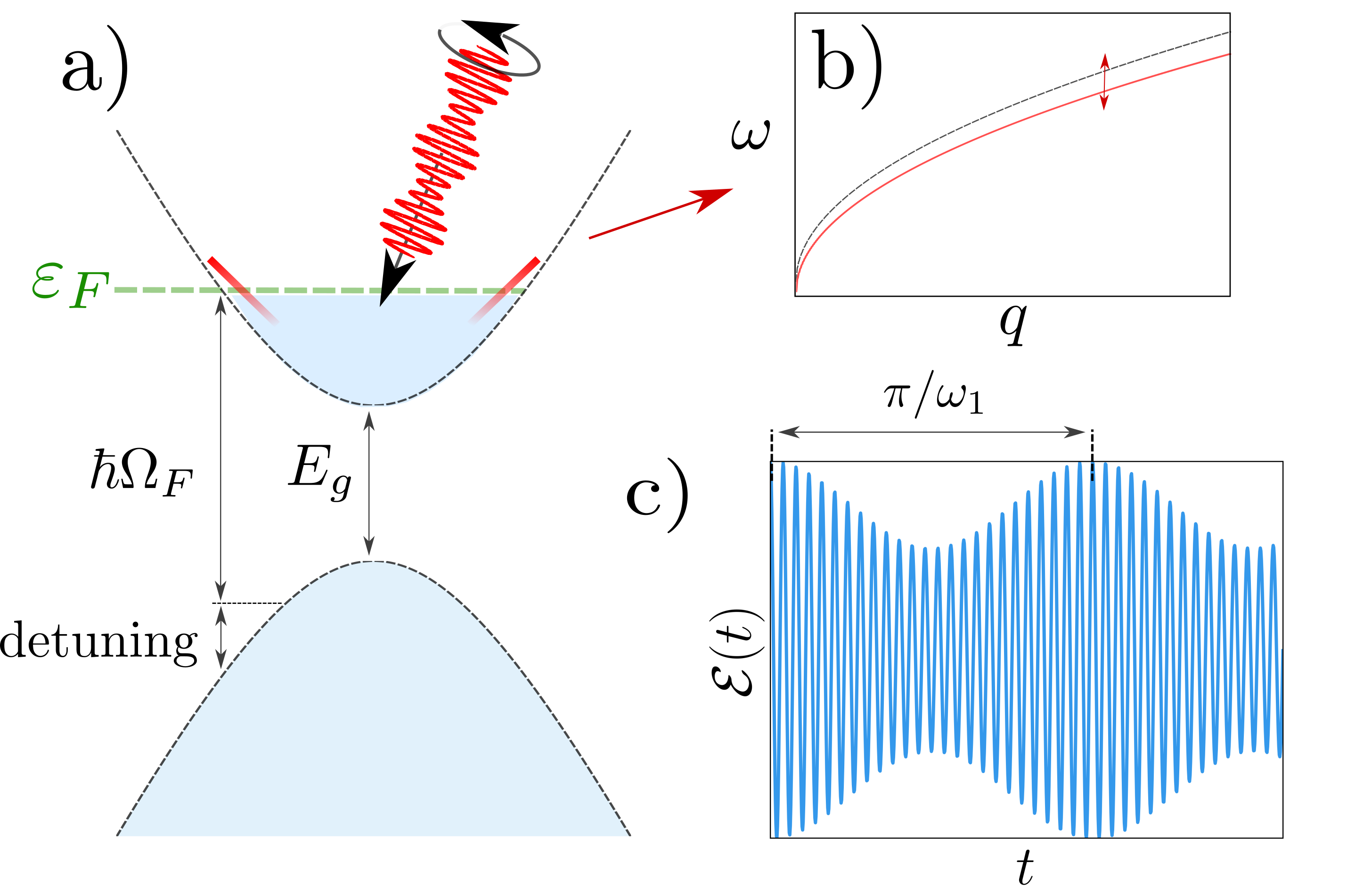
Figure 1: Floquet engineering and MFPD. a) The band structure of a gapped Dirac material (grey) with gap $E_{g}$ driven with circularly polarized infrared light. The driving frequency $\Omega_{F}$ and the Fermi energy $\varepsilon_{F}$ are chosen such that single photon absorption and particle-hole creation with energy transfer $\hbar\Omega_{F}$ is blocked by the Fermi see (detuning). The driving leads to a change of the group velocity at the Fermi surface (red). b) This change results in a shift of the plasmon dispersion $\omega_{\mathrm{pl}}\left(q\right)$. c) Modulating the amplitude of the Floquet drive with a frequency $\omega_{1}\ll\Omega_{F}$ will lead to an oscillating Fermi velocity. This oscillation induces a parametric resonance of the plasmon modes.

Interesting effects can also be achieved with pulsed signals. In analogy to recent experiments with surface waves in classical liquids (bacot2016time_mirror_water, ), we propose, that pulses can be used to induce time reversal of propagating plasmon wave packets. As we elaborate below, a high frequency pulse will split a propagating low frequency plasmon wave packet into two parts. While one part will continue to propagate in the initial direction, the other will evolve backwards in time and propagate towards its origin (see Fig. 2). We suggest that pulse induced time reversal is a promising way to control the propagation of THz plasmons with off-resonant, high frequency light – an effect that is mediated by the Floquet reshaping of the electron dispersion.

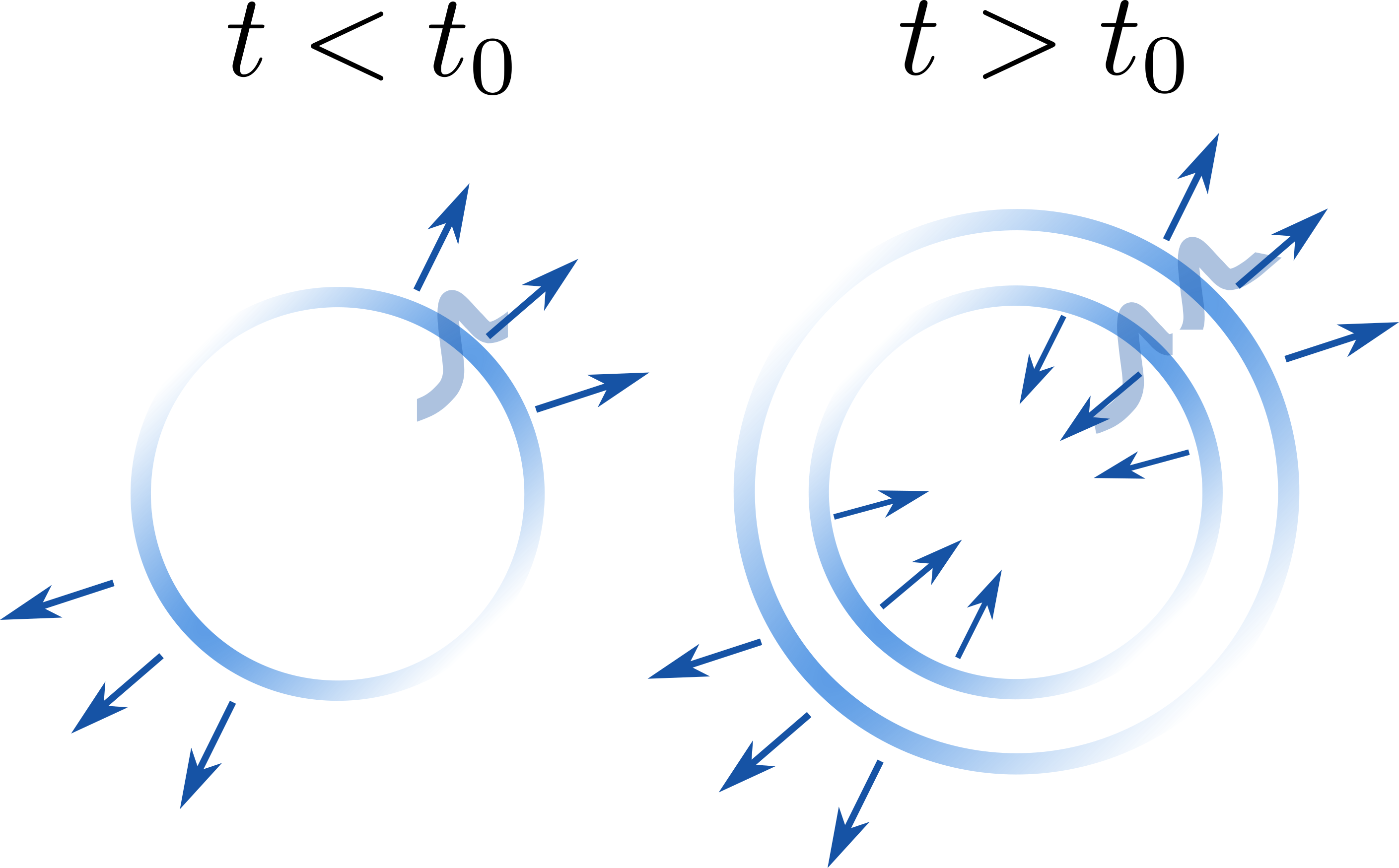
Figure 2: Pulse induced time reversal of a propagating spherical plasmon wave packet: A high frequency pulse is applied at time $t_{0}$. The abrupt change of the electrons’ Fermi velocity and effective mass results in a splitting of the wavefront into parts, with one part propagating back towards the origin.

Modulated Floquet parametric driving: Floquet engineering of time varying materials.

In this section we show how MFPD can be used to create a time varying plasmonic medium. For concreteness, we study a gapped Dirac Hamiltonian which describes electrons near the Fermi level of a two dimensional material – e.g. a transition metal dichalcogenide or black phosphorus (chaves2020_2d_semiconductors_bandgaps, ; kim2015dirac_black_phosphorus, ; chaves2017_excitonic_tmdcs, ):

$$H=\sum_{\mathbf{k}}\mathbf{c}_{\mathbf{k}}^{\dagger}\left[H_{0}\left(\mathbf{k}\right)+H_{d}\left(t\right)\right]\mathbf{c}_{\mathbf{k}}+\sum_{\mathbf{q}}V\left(\mathbf{q}\right)\rho_{\mathbf{q}}\rho_{-\mathbf{q}}.$$ (2)

We focus on a single valley and write $H_{0}=\mathbf{d}\cdot\boldsymbol{\sigma}$ with $\mathbf{d}=\left[\lambda k_{x},\lambda k_{y},E_{g}/2\right]$, where, $E_{g}$ is the energy gap between the two bands, $\boldsymbol{\sigma}$ is a Pauli vector describing pseudospin-orbit coupling, $\mathbf{c}_{\mathbf{k}}^{\dagger}$,$\mathbf{c}_{\mathbf{k}}$ are electron creation and annihilation operators, $\rho_{\mathbf{q}}=\sum_{\mathbf{k}}\mathbf{c}_{\mathbf{k}+\mathbf{q}}^{\dagger}\mathbf{c}_{\mathbf{k}}$ is the density operator and $V\left(\mathbf{q}\right)=2\pi/q$ is the 2D Fourier transform of the Coulomb potential.

The driving Hamiltonian is derived from minimal coupling: $H_{d}\left(\mathbf{k}\right)=e\mathbf{A}\cdot\nabla_{\mathbf{k}}H_{0}$. We assume circularly polarized light with an amplitude $\mathcal{E}$ described by the vector potential $\mathbf{A}=\left(\mathcal{E}/\Omega_{F}\right)\left[-\sin\Omega_{F}t,\cos\Omega_{F}t,0\right]$. For the subsequent analysis it is useful to change to the rotating frame by applying the unitary transformation $U=e^{i\hat{\mathbf{d}}\cdot\boldsymbol{\sigma}\Omega_{F}t}$ to Eq. (2) (rudner2020band_engineering, ). The spectrum of the single particle part of $H$ in the rotating frame reads

$$\varepsilon_{k}\approx\sqrt{\left(\left|\mathbf{d}\right|-\hbar\frac{\Omega_{F}}{2}\right)^{2}+\frac{e^{2}\mathcal{E}^{2}\lambda^{2}}{4\Omega^{2}\hbar^{2}}\left(2-\frac{E_{g}}{\left|\mathbf{d}\right|}\right)}$$ (3)

for $\lambda k/\left|\mathbf{d}\right|\ll 1$. Deriving Eq. (3), we used the rotating wave approximation and ignored terms oscillating at higher frequencies in the rotating frame (rudner2020band_engineering, ; lindner2011floquet, ).

To avoid direct single photon absorptions, which are a dominant source of heating in Floquet engineered systems (seetharam2015baths_controlled_floquet_population, ; esin2018q_steady_state_topo_ins, ; esin2021_liquid_crystal, ), we suggest to operate in an off-resonant regime, where the Fermi surface lies close to, but above the single photon resonance (see Fig.1). In this off-resonant regime, all states supporting excitations of an electron by photons with an energy of $\hbar\Omega_{F}$ and near-zero momentum tranfer are blocked. Processes involving the absorption of multiple photons are suppresed to second order in the small ratio of driving amplitude over driving frequency $e\mathcal{E}\lambda/\Omega^{2}\hbar^{2}$(seetharam2015baths_controlled_floquet_population, ; esin2021_liquid_crystal, ). Floquet engineering in this regime has recently been demonstrated experimentally (zhou2023black_phosphorus_floquet, ).

We employ MFPD by subjecting the Floquet drive amplitude $\mathcal{E}$ to a slow modulation. Expanding the dispersion relation around the Fermi momentum we find $\varepsilon_{k}\approx\hbar v_{F}\left(\mathcal{E},\Omega_{F}\right)\left(k-k_{F}\right)+\varepsilon_{k_{F}}\left(\mathcal{E},\Omega_{F}\right).$ Here, the Fermi velocity $v_{F}\left(\mathcal{E},\Omega_{F}\right)$ depends on the amplitude and frequency of the Floquet drive. A slow, time periodic modulation of $\mathcal{E}$ according to $\mathcal{E}\left(t\right)=\bar{\mathcal{E}}+\delta\mathcal{E}\cos\left(2\omega_{1}t\right),$where $\omega_{1}\ll\Omega_{F}$, will result in an oscillating Fermi velocity. For our purposes, it will be convenient to parametrize this time dependence as an oscillation of the effective mass $m^{*}=\hbar k_{F}/v_{F}\left(\mathcal{E},\Omega_{F}\right)$:

$$m^{*}\left(t\right)=\bar{m}^{*}\left(1+h\cos\left(2\omega_{1}t\right)\right).$$ (4)

Here, $h$ is a small dimensionless number quantifying the amplitude of the oscillatory component of the effective mass. Below, we estimate that for reasonable driving strenghts $h$ is of the order of $10^{-2}$.

Momentum-gapped states.

We now investigate the influence of the oscillating effective mass of Eq. (4) on the dispersion relation of plasmons in a Coulomb interacting 2D electron gas. The plasmon dynamics can be inferred from charge and momentum conservation (Eguiluz1976hydrodynamicPlasmons, ; Forster, ; lucas2015memory, ; kiselev2021_superdiffusive_modes, ). The continuity equation for the charge density $\rho$ reads

$$\partial_{t}\rho\left(\mathbf{x},t\right)=-\nabla\cdot\mathbf{j}\left(\mathbf{x},t\right).$$ (5)

Here, $\mathbf{j}$ is the electric current. It is related to the momentum density $\mathbf{p}$ via

$$\mathbf{p}\left(\mathbf{x},t\right)=\frac{m^{*}\left(t\right)}{e}\mathbf{j}\left(\mathbf{x},t\right).$$ (6)

An inhomogeneous charge distribution $\rho\left(\mathbf{x},t\right)$ will induce potential differences in the system which will accelerate the electrons according to Newton’s law:

$$\partial_{t}\mathbf{p}\left(\mathbf{x},t\right)=-\rho\left(\mathbf{x},t\right)\nabla\phi\left(\mathbf{x},t\right).$$ (7)

The electrostatic potential is given by

$$\phi\left(\mathbf{x},t\right)=\frac{1}{\varepsilon}\rho\left(\mathbf{x},t\right)\nabla\int d^{2}x^{\prime}\frac{\rho\left(\mathbf{x}^{\prime},t\right)}{\left|\mathbf{x}-\mathbf{x}^{\prime}\right|},$$ (8)

where $\varepsilon$ is the dielectric constant. The integral is taken over the whole sample. Inserting Eq. (6) into (7), taking the gradient and using Eq. (5), we find

$$\partial_{t}m^{*}\left(t\right)\partial_{t}\rho\left(\mathbf{x},t\right)=\frac{e}{\varepsilon}\nabla\cdot\rho\left(\mathbf{x},t\right)\nabla\int d^{2}x^{\prime}\frac{\rho\left(\mathbf{x}^{\prime},t\right)}{\left|\mathbf{x}-\mathbf{x}^{\prime}\right|}.$$ (9)

We separate the oscillating part of $\rho$ from the homogeneous background $\bar{\rho}$ and write $\rho=\bar{\rho}+\delta\rho$. Linearizing Eq. (9) in $\delta\rho$, and assuming plane-wave solutions $\delta\rho\left(\mathbf{x}\right)=\delta\rho_{\mathbf{q}}\exp\left(i\mathbf{q}\cdot\mathbf{x}\right)$, we obtain Eq. (1).

The plasmon dispersion $\omega_{\mathrm{pl}}\left(q\right)$ is given by

$$\omega_{\mathrm{pl}}\left(q\right)=\sqrt{\frac{e\rho_{0}}{m^{*}\varepsilon}q^{2}V\left(q\right)},$$ (10)

where $V\left(q\right)$ is the Fourier transform of the Coulomb potential.

We consider a quasi one-dimensional, waveguide-like set-up of infinite length and width $l$ (see Fig. 11). For this slab geometry we find

$$V\left(q\right)\approx\int_{0}^{l}dy\int_{-\infty}^{\infty}dx\frac{e^{i\mathbf{q}\cdot\mathbf{x}}}{\left|\mathbf{x}\right|}\approx 2l\left|\ln\frac{\left|q\right|l}{4}\right|$$ (11)

for $q\ll 1/l$, where the wavevector is chosen to align with the $x$-direction. The precise geometry of the device is not very important for the physics presented here, and the calculations would be very similar for an infinite 2D sample with $V\left(q\right)=2\pi/q$, except that we would need to keep track of the vector nature of $\mathbf{q}$.

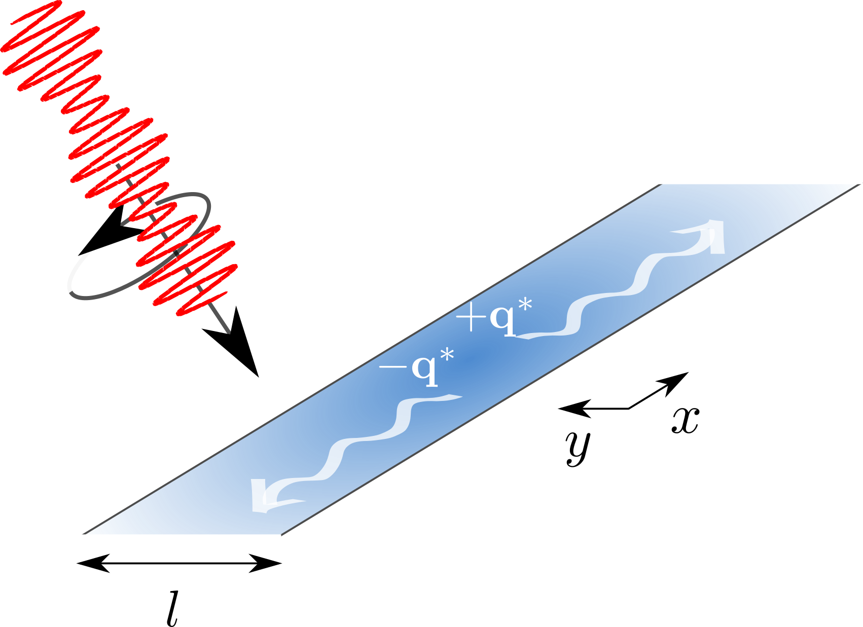
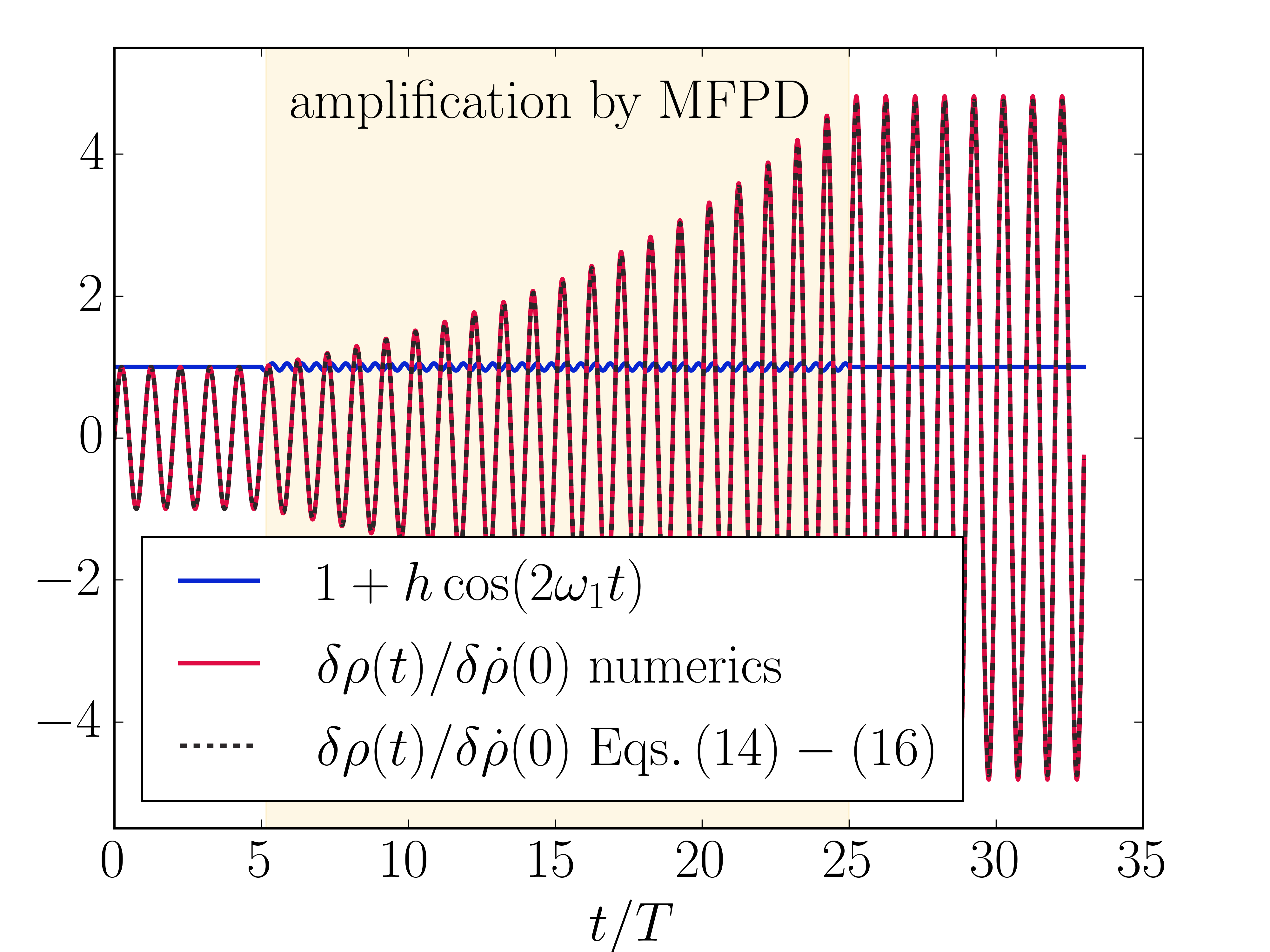
Figure 3: Left: the quasi one-dimensional slab geometry considered in Eq. (11). Due to momentum conservation, plasmons created by MFPD come in entangled pairs with momenta $\pm q^{*}$. Right: Amplification of a plasmon mode by MFPD. The relative oscillation of the effective mass $m^{*}$ is shown in blue. The red curve shows the numerical solution to Eq. (1). The dashed black curve shows the analytical approximation.

We want to study the behavior of $\delta\rho_{q}$ in the vicinity of the parametric resonance, where $\left|\omega_{\mathrm{pl}}\left(q\right)-\omega_{1}\right|\approx h\omega_{1}$. Using the ansatz $\delta\rho_{q}=a_{q}\left(t\right)\cos\left(\omega_{1}t\right)+b_{q}\left(t\right)\sin\left(\omega_{1}t\right)$, where the slowly varying coefficients are given by $a_{q}\left(t\right)=\tilde{a}e^{st}$ and $b_{q}\left(t\right)=\tilde{b}e^{st}$, we find (see supplementary material)

$$s_{\pm}\left(q\right)=\pm\frac{\omega_{1}}{2}\sqrt{\frac{1}{4}h^{2}-\left(\frac{\omega_{\mathrm{pl}}^{2}\left(q\right)-\omega_{1}^{2}}{\omega_{1}^{2}}\right)^{2}}.$$ (12)

For $\left|\omega_{\mathrm{pl}}^{2}\left(q\right)-\omega_{1}^{2}\right|>\omega_{1}^{2}h/2$ the exponent is imaginary, corresponding to dispersive plane-wave solutions, whereas for $\left|\omega_{\mathrm{pl}}^{2}\left(q\right)-\omega_{1}^{2}\right|<\omega_{1}^{2}h/2$, we find exponentially growing (or decaying) unstable non-dispersive solutions oscillating at the frequency $\omega_{1}$. This results in a momentum gapped dispersion, similar to the one appearing in so called photonic time crystals (lustig2018topological_photonic_time_crystal, ; galiffi2022photonics_time_varying_ptc, ). In the quasi 1D slab geometry, the gap is centered at the wavevectors $\pm q^{*}$, where $q^{*}$ is determined by the resonance condition

$$\omega_{\mathrm{pl}}\left(q^{*}\right)=\omega_{1}.$$ (13)

Notice that Eq. (1) is invariant with respect to time translations by $T=\pi/\omega_{1}$. This symmetry is broken by the system’s response – a feature that is known from discrete time crystals (else2020discrete_time_cryst_review, ; else2016floquet_discrete_time_crystals, ; yao2017discrete_time_crystal_original, ; zhang2017observation_discrete_time_crystal, ; kyprianidis2021observation_discrete_time_crystal, ; natsheh2021critical_properties_time_crystal, ; yao2020classical_discrete_time_crystal, ) and generic to parametric resonances. The momentum gap and the dispersion in the vicinity of the gap are shown in Fig. 4.

So far we did not consider the finite lifetime of plasmons. We assume that the main source of damping are momentum relaxing collisions (e.g. with phonons or crystal defects). For small $q$, the plasmon dispersion lies outside the particle-hole continuum and Landau damping can be neglected. The momentum density of plasmons is thus not conserved, but rather decays at a rate $\gamma$. To model this effect, we add the term $-\gamma\mathbf{p}$ to the right hand side of Eq. (7). To first order in $\gamma$, $s_{\pm}\left(q\right)$ in Eq. (12) obtains negative real part of $-\gamma/2$ (see supplementary material). The instability condition $\mathrm{Re}\left(s_{\pm}\right)>0$ is realized in a narrow region around $q^{*}$ for

$$h>2\gamma/\omega_{1}.$$ (14)

Interestingly, even if $h<2\gamma/\omega_{1}$ holds, the momentum-gap remains intact. The gap then hosts non-dispersive modes with decay rates $-\gamma/2\pm\omega_{1}h^{2}/4$ at $q=q^{*}$.

Band structure of the plasmonic time varying medium.

Eq. (12) suggests that the opening of the momentum gap is associated with the joining of two branches of the plasmon dispersion described by the plus and minus signs. To interpret the two branches, it is useful to write the solution of Eq. (12) in the form known from Floquet’s theorem (ince1956o_ODE_book, ). We find

$$\delta\rho_{q}=e^{i\epsilon_{\mathrm{pl}}\left(q\right)t}u_{\epsilon_{\mathrm{pl}}}\left(t\right),$$ (15)

where $\epsilon_{\mathrm{pl}}\left(q\right)$ is the plasmon quasi-dispersion that determines wave propagation once the periodic modulation is switched on . In the vicinity of the gap we have

$$\epsilon_{\mathrm{pl},\pm}\left(q\right)=-is_{\pm}\left(q\right)+i\omega_{1},$$ (16)

and

$$u_{\epsilon_{\mathrm{pl}}}\left(t\right)=\frac{1}{2}\left[\tilde{a}_{\epsilon_{\mathrm{pl}}}\left(1+e^{-2i\omega_{1}t}\right)-i\tilde{b}_{\epsilon_{\mathrm{pl}}}\left(1-e^{-2i\omega_{1}t}\right)\right],$$ (17)

where in accordance with Floquet’s theorem we find $u_{\epsilon_{\mathrm{pl}}}\left(t+\pi/\omega_{1}\right)=u_{\epsilon_{\mathrm{pl}}}\left(t\right)$. Keeping terms of oder $\mathcal{O}\left(h^{2}\right)$, one finds that for small $q$, i.e. away from the momentum gap, the quasi-dispersions of the $\pm$-modes are given by

$$\epsilon_{\mathrm{pl},+} \approx i\omega_{\mathrm{pl}}\left(q\right)/\sqrt{1+h^{2}/4}$$

$$\epsilon_{\mathrm{pl},-} \approx 2i\omega_{1}-i\omega_{\mathrm{pl}}\left(q\right)/\sqrt{1+h^{2}/4}.$$ (18)

While $\epsilon_{\mathrm{pl},+}$ reduces to $\omega_{\mathrm{pl}}\left(q\right)$ in the absence of MFPD ($h=0$), for the $\epsilon_{\mathrm{pl},-}$ mode, we find that $\tilde{b}_{\epsilon_{\mathrm{pl}}}=-i\tilde{a}_{\epsilon_{\mathrm{pl}}}$ for $q\approx 0$. This gives $\delta\rho_{q}\approx a_{\epsilon_{\mathrm{pl}},-}e^{-i\omega_{\mathrm{pl}}\left(q\right)t/\sqrt{1+h^{2}/4}}$, showing that the $\epsilon_{\mathrm{pl},-}$ and $\epsilon_{\mathrm{pl},+}$ modes describe equivalent, counter-propagating waves. Indeed, according to Floquet’s theorem, the quasi-dispersion $\epsilon_{\mathrm{pl}}$ is defined modulo a frequency shift of $2\omega_{1}$, which plays the role of a reciprocal unit vector along the frequency axis. We chose the Brillouin zone such that it covers frequencies from $0$ to $2\omega_{1}$. In analogy with the Bloch theory of electrons in periodic lattices, the opening of the momentum gap can be interpreted as an avoided level crossing of the $\epsilon_{\mathrm{pl},\pm}$-modes. The plasmonic band structure is shown in Fig. 4.

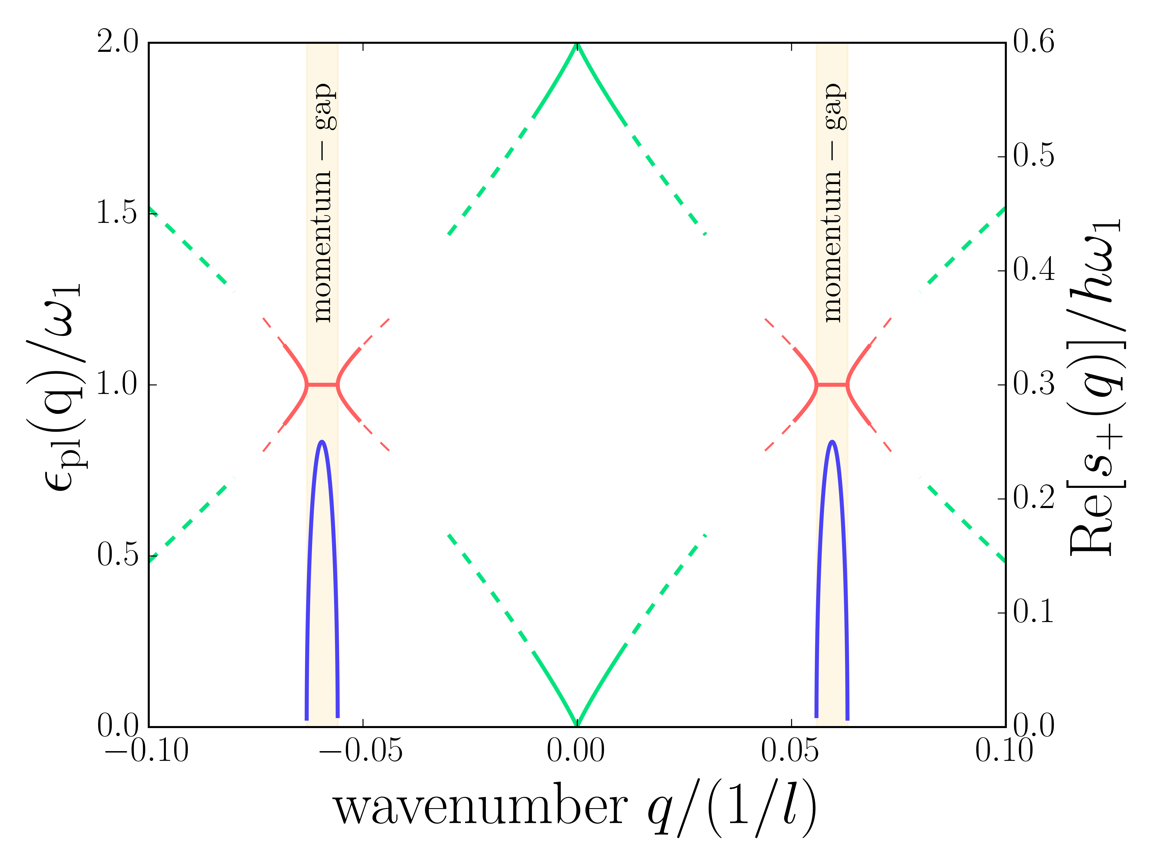
Figure 4: Dispersion of the plasmonic timy varying medium. The modulated Floquet drive couples to plasmon modes and induces gaps (yellow bars) near the resonance $\omega_{1}=\omega_{\mathrm{pl}}\left(q\right)$. In the vicinity of the gaps, the modes are given by Eq. (12) (red curves). Away from the gap, the drive-induced changes to the dispersion are small (green curves). The growth rate of the unstable modes $\mathrm{Re}\left[s_{+}\left(q\right)\right]$ is shown in blue.

The exponential growth of unstable plasmonic modes must saturate eventually. In the simplest scenario, MFPD can be switched off as soon as a predetermined amplification threshold amplitude is reached (see Fig. 3). More generically, the nonlinearities of the system will provide a stabilyzing mechanism (kovacic2018nonlinear_mathieu, ; kiselev2023MFPD, ; chen_vinals_1999_faraday_pattern_sel, ), leading to new correlated steady states characterized by the breaking of translation symmetry and the formation of patterns with periodicity $2\pi/q^{*}$ (kiselev2023MFPD, ). As has been shown for PTCs, nonlinearities can also lead to the formation of exotic superluminal solitons (pan2022superluminal_k-gap_solitons, ).

Production of entangled plasmon pairs.

Since the momentum supplied by the optical drive is negligable, plasmons can only be produced in pairs with opposite momenta $\pm\hbar q$. This results in the generation of entangled plasmon pairs. To see this, we find the Hamiltonian leading to Eq. (1) and then apply a second quantization procedure following Refs. (mendoncca2005_entangled_photon_pairs, ; lyubarov2022photonic_time_crystal_amplified, ). Details are given in the supplementary material. For the driven plasmon Hamiltonian in the interaction representation we find

$$H_{\mathrm{pl},\mathrm{int}}\approx\frac{h}{4}\hbar\omega_{1}\left(a_{q^{*}}^{\dagger}a_{-q^{*}}^{\dagger}+a_{-q^{*}}a_{q^{*}}\right),$$ (19)

where we focused on the resonant wavenumber $q^{*}$ and a small modulation strength $h\ll 1$.

Applied to the vacuum, the time evolution operator $U_{\mathrm{pl,int}}\left(t,0\right)=\exp\left(-tH_{\mathrm{pl},\mathrm{int}}/\hbar\right)$ generates a non-factorizable two mode squeezed state $\ket{\psi_{\mathrm{pl}}\left(t\right)}=U_{\mathrm{pl,int}}\left(t,0\right)\ket{0,0}$ in the basis $\ket{n_{q},n_{-q}}$ (gerry2005introductory_quantum_optics, ), where $n_{q}$ gives the number of plasmons in the state $q$:

$$\ket{\psi_{\mathrm{pl}}\left(t\right)}=\frac{1}{\cosh\left(\frac{h\omega_{1}t}{4}\right)}\sum_{n=0}\tanh^{n}\left(\frac{h\omega_{1}t}{4}\right)|n_{q},n_{-q}\rangle.$$ (20)

The total number of plasmons $\langle N_{\pm q}\rangle=\bra{\psi_{\mathrm{pl}}\left(t\right)}a_{\pm q}^{\dagger}a_{\pm q}\ket{\psi_{\mathrm{pl}}\left(t\right)}\sim\exp\left(h\omega_{1}t/2\right)$ grows exponentially in accordance with the classical result of Eq. (12). We note that the generation of entangled plasmon pairs has been discussed previously in Ref. (sun2022graphene_entangled_plasmon_pairs, ), where the authors suggested to excite the longitudinal plasmon modes of a graphene ribbon via their copling to a resonantly pumped transverse mode. Ref. (sun2022graphene_entangled_plasmon_pairs, ) also discusses possible modes of detection of plasmon entanglement.

Phase sensitive parametric amplification

A single mode plasmonic time varying medium resonator can act as a phase sensitive parametric amplifier. As a toy model, we consider a THZ waveguide coupled to an MFPD driven resonator at $x=0$. The waveguide is described by the equation

$$\frac{\partial^{2}Q}{\partial t^{2}}-c^{2}\frac{\partial^{2}Q}{\partial x^{2}}=-g\delta\dot{\rho}\delta\left(x\right),$$ (21)

while the equation for the oscillator reads

$$\partial_{t}\left(1+h\cos 2\omega_{1}t\right)\partial_{t}\delta\rho+\gamma\delta\dot{\rho}=\Gamma\dot{Q}\left(x=0\right).$$ (22)

Here, $c$ is the speed of wave propagation, $g$ and $\Gamma$ characterize the coupling between resonator and waveguide. We chose the MFPD frequency $\omega_{1}$ to coincide with the resonance frequency. Let us, for simplicity, assume that the waves transmitted through the waveguide also have a frequency $\omega_{1}$. For $x<0$, the waveguide field is written as

$$Q\left(x<0\right)=A\cos\left(\omega_{1}t-kr+\delta_{1}\right)+B\cos\left(\omega_{1}t+kr+\delta_{2}\right).$$ (23)

For $x>0$, we write

$$Q\left(x>0\right)=C\cos\left(\omega_{1}t-kr-\delta_{3}\right).$$ (24)

$A$, $B$, and $C$ describe incident, reflected and transmitted wave amplitudes respectively. In the supplementary material, we calculate the amplitudes as a function of the phase of the incomming wave $\delta_{1}$. We find that, roughly, $C\sim 1/\left(4\tilde{\gamma}^{2}/\omega^{2}-h^{2}\right)$, where $\tilde{\gamma}=\gamma+g\Gamma/\left(2c\omega_{1}\right)$ describes the losses of the resonator to both, internal damping and the waveguide. Thus, amplification is strongest near the critical value $h=2\tilde{\gamma}/\omega$. Fig. 5 shows the amplitude and phase of the amplified, transmitted signal as a function $\delta_{1}$. Both quantities show a strong dependence on the phase of the incident wave $\delta_{1}$ with respect to the MFPD drive.

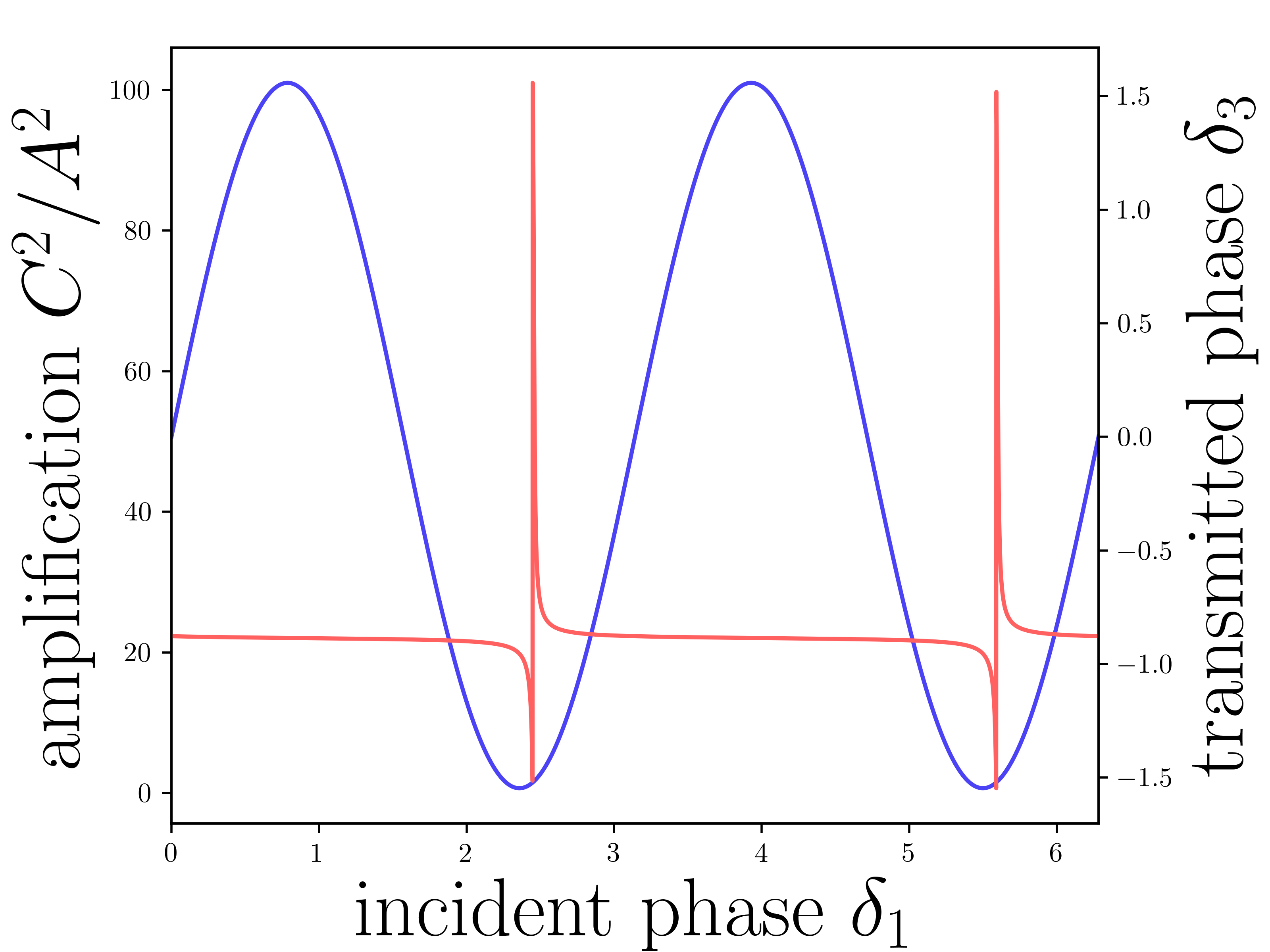
Figure 5: Normalized amplitude $C$ (blue) and phase $\delta_{3}$ (red) of the transmitted signal in the near-critical regime $h\lesssim 2\tilde{\gamma}/\omega_{1}$. Both are strongly dependent on the phase $\delta_{1}$ of the incident signal with respect to the MFPD driving. For the plot, we chose $h\approx 0.97\cdot 2\tilde{\gamma}/\omega_{1}$.

Pulse induced time reversal

So far we have considered the action of a periodic oscillation of the effective mass $m^{*}\left(t\right)$ resulting from an amplitude modulated high frequency Floquet driving. In this section, we show how a pulse induced, abrupt change of $m^{*}\left(t\right)$ can time reverse propagating plasmon wave packeges – the effect shown in Fig.2. We consider a pulse with peak amplitude $\mathcal{E}_{0}$, center frequency $\Omega_{F}$ and duration $\Delta t$. As shown in the supplement, the effect of such a pulse at time $t=t_{0}$ on the effective mass can be described by the formula

$$m^{*}\left(t\right)=\bar{m}^{*}\left(1+\bar{h}\delta\left(t-t_{0}\right)\right),$$ (25)

where $\bar{h}$ is an amplitude characterizing the impact of the pulse. Let us, for a moment, depart from the qusi-1D situation of Fig.3 and focus on a 2D system. Plasmon propagation in the presence of a pulse at $t=t_{0}$ is described by the equation

$$\partial_{t}^{2}\delta\rho_{\mathbf{q}}+\omega_{\mathrm{pl}}^{2}\left(q\right)\delta\rho{}_{\mathbf{q}}=-\bar{h}\partial_{t}\delta\left(t-t_{0}\right)\partial_{t}\delta\rho_{\mathbf{q}}.$$ (26)

Considering an initial propagating wave packet of the form $\delta\rho_{i}\left(\mathbf{x},t\right)=\int\frac{d^{2}q}{2\pi}\phi_{i}\left(\mathbf{q}\right)e^{i\mathbf{q}\cdot\mathbf{x}-i\omega_{\mathrm{pl}}\left(q\right)t}$, we find that, to first order in $\bar{h}$, the plasmon field at all times is given by

$$\delta\rho\left(\mathbf{x},t\right) \approx\delta\rho_{i}\left(\mathbf{x},t\right)$$

$$+\frac{i}{2}\bar{h}\Theta\left(t-t_{0}\right)\partial_{t}\left[\delta\rho_{i}\left(\mathbf{x},2t_{0}-t\right)+\delta\rho_{i}\left(\mathbf{x},t\right)\right].$$ (27)

The second right hand side term describes the impact of the pulse, with the first term in square brackets corresponding to a signal propagating backwards in time. Let us denote this part by $\delta\rho_{\mathrm{rev}}\left(\mathbf{x},t\right)$. In the supplement, we demonstrate that, for a narrow wave packet, the time reversed part is given by

$$\delta\rho_{\mathrm{rev}}\left(\mathbf{x},t\right)\approx A\left(q_{0}\right)\delta\rho_{i}\left(\mathbf{x},-t\right).$$ (28)

Here, $A\left(q_{0}\right)=\frac{1}{2}\omega_{\mathrm{pl}}\left(q_{0}\right)\bar{h}e^{-i2\omega_{\mathrm{pl}}\left(q_{0}\right)t_{0}}$ is a complex amplitude and $q_{0}$ is the central wavenumber of the package.

Discussion.

Recent ARPES measurements in electron doped black phosphorus – a Dirac-like gapped semiconductor – demonstrated a reshaping of the bandstructure by light in the off-resonant regime with blocked direct photoexcitations (zhou2023black_phosphorus_floquet, ). Thus, the regime of operation for MFPD induced plasmonic time varying materials is within experimental reach. While we used the example of a gapped Dirac system for our calculations, the outlined effects could be achieved in wider class of materials. An obvious candidate is graphene, which is an important system for both plasmonics and Floquet engineering (ni2018_plasmon_quality_factor_graphene, ; kitagawa2011floquetinduced, ; mciver2020light_anomaouls_hall_graphene, ).

With parameters given in the supplementary material and using Eq. (14), we estimate the critical driving strength to be $\mathcal{\bar{E}}\approx 4\cdot 10^{5}\,\mathrm{V}/\mathrm{m}$. The corresponding intensity is by a factor of $10^{4}$ smaller than in current solid state Floquet engineering experiments (wang2013_floquet-bloch_states_observation, ; mahmood2016selective_scattering_floquet-bloch_volkov, ; mciver2020light_anomaouls_hall_graphene, ; zhou2023black_phosphorus_floquet, ). We assumed a plasmon quality factor of $Q=\omega_{1}/\gamma\approx 10^{2}$ (ni2018_plasmon_quality_factor_graphene, ). $Q$-factors of $10^{3}-10^{4}$ are believed to be achievable on the basis of theoretical predictions (principi2013intrinsic_graphene_plasmon_quality_factor, ; ni2018_plasmon_quality_factor_graphene, ). This could help to further reduce the required laser intensity. Finally, we note that the realization of plasmonic time reversal requires only pulsed signals and could be demonstrated in set-ups similar to the ones used in most Floquet experiments (mciver2020light_anomaouls_hall_graphene, ; zhou2023black_phosphorus_floquet, ; mahmood2016selective_scattering_floquet-bloch_volkov, ; wang2013_floquet-bloch_states_observation, ).

Supplementary Material

Supplementary Sec..1 Solving the time varying plasmon equation

Here we show details of our solution to Eq. (1) of the main text using the ansatz

$$\delta\rho=a\left(t\right)\cos\left(\omega_{1}t\right)+b\left(t\right)\sin\left(\omega_{1}t\right).$$ (S 1)

Inserting Eq. (S 1) this into Eq. (1) results in

$$\partial_{t}\left(1+\frac{\delta m^{*}\left(t\right)}{m^{*}}\right)\partial_{t}\delta\rho =-2\omega_{1}h\sin\left(2\omega_{1}t\right)\delta\dot{\rho}+\left(1-h\cos\left(2\omega_{1}t\right)\right)\delta\ddot{\rho}$$

$$=-2\omega_{1}h\sin\left(\omega_{1}t\right)\left[\dot{a}\cos\left(\omega_{1}t\right)+\dot{b}\sin\left(\omega_{1}t\right)\right.$$

$$\qquad\left.-a\omega_{1}\sin\left(\omega_{1}t\right)+b\omega_{1}\cos\left(\omega_{1}t\right)\right]$$

$$\qquad+\left(1-h\cos\left(2\omega_{1}t\right)\right)\left[\ddot{a}\cos\left(\omega_{1}t\right)+\ddot{b}\sin\left(\omega_{1}t\right)\right.$$

$$\qquad-2\dot{a}\omega_{1}\sin\left(\omega_{1}t\right)+2\dot{b}\omega_{1}\cos\left(\omega_{1}t\right)$$

$$\qquad\left.-a\omega_{1}^{2}\cos\left(\omega_{1}t\right)-b\omega_{1}^{2}\sin\left(\omega_{1}t\right)\right]$$

$$\partial_{t}\left(1+\frac{\delta m^{*}\left(t\right)}{m^{*}}\right)\partial_{t}\delta\rho \approx-\omega_{1}h\left[\dot{a}\sin\left(\omega_{1}t\right)+\dot{b}\cos\left(\omega_{1}t\right)\right.$$

$$\qquad\left.-a\omega_{1}\cos\left(\omega_{1}t\right)+b\omega_{1}\sin\left(\omega_{1}t\right)\right]$$

$$\qquad+\left[\ddot{a}\cos\left(\omega_{1}t\right)+\ddot{b}\sin\left(\omega_{1}t\right)\right.$$

$$\qquad-2\dot{a}\omega_{1}\sin\left(\omega_{1}t\right)+2\dot{b}\omega_{1}\cos\left(\omega_{1}t\right)$$

$$\qquad\left.-a\omega_{1}^{2}\cos\left(\omega_{1}t\right)-b\omega_{1}^{2}\sin\left(\omega_{1}t\right)\right]$$

$$\qquad+\left(h/2\right)\left[\ddot{a}\cos\left(\omega_{1}t\right)-\ddot{b}\sin\left(\omega_{1}t\right)\right.$$

$$\qquad+2\dot{a}\omega_{1}\sin\left(\omega_{1}t\right)+2\dot{b}\omega_{1}\cos\left(\omega_{1}t\right)$$

$$\qquad\left.-a\omega_{1}^{2}\cos\left(\omega_{1}t\right)+b\omega_{1}^{2}\sin\left(\omega_{1}t\right)\right]$$

$$\gamma\partial_{t}\delta\rho =\gamma\left[\dot{a}\cos\left(\omega_{1}t\right)+\dot{b}\sin\left(\omega_{1}t\right)\right.$$

$$\quad\left.-a\omega_{1}\sin\left(\omega_{1}t\right)+b\omega_{1}\cos\left(\omega_{1}t\right)\right].$$

Comparing the coefficients in front of the sine and cosine functions we find the equations for the amplitudes $a\left(t\right)$ and $b\left(t\right)$:

$$-\omega_{1}h\left(\dot{a}+\omega_{1}b\right)+\ddot{b}-2\dot{a}\omega_{1}-b\omega_{1}^{2}+\left(h/2\right)\left(-\ddot{b}+2\dot{a}\omega_{1}+b\omega_{1}^{2}\right)+\gamma\left(\dot{b}-a\omega_{1}\right)+\omega_{\mathrm{pl}}^{2}\left(q\right)b =0$$

$$-\omega_{1}h\left(\dot{b}-\omega_{1}a\right)+\ddot{a}+2\dot{b}\omega_{1}-a\omega_{1}^{2}+\left(h/2\right)\left(\ddot{a}+2\dot{b}\omega_{1}-a\omega_{1}^{2}\right)+\gamma\left(\dot{a}+b\omega_{1}\right)+\omega_{\mathrm{pl}}^{2}\left(q\right)a =0$$

anticipating $a\sim b\sim e^{st}$, where $s\sim\omega_{1}h$ and ignoring $\mathcal{O}\left(h^{2}\right)$ and higher, we find

$$-\omega_{1}^{2}hb/2-2\dot{a}\omega_{1}-\gamma a\omega_{1}+\left(\omega_{\mathrm{pl}}^{2}\left(q\right)-\omega_{1}^{2}\right)b =0$$

$$\omega_{1}^{2}ha/2+2\dot{b}\omega_{1}+\gamma b\omega_{1}+\left(\omega_{\mathrm{pl}}^{2}\left(q\right)-\omega_{1}^{2}\right)a =0.$$ (S 2)

Next we use the ansatz $a=\tilde{a}e^{st}$, $b=\tilde{b}e^{st}$:

$$\left[\begin{array}[]{cc}-2s\omega_{1}-\gamma\omega_{1}&-\frac{1}{2}\omega_{1}^{2}h+\left(\omega_{\mathrm{pl}}^{2}-\omega_{1}^{2}\right)\\ \frac{1}{2}\omega_{1}^{2}h+\left(\omega_{\mathrm{pl}}^{2}-\omega_{1}^{2}\right)&2s\omega_{1}+\gamma\omega_{1}\end{array}\right]\left[\begin{array}[]{c}a\\ b\end{array}\right]=0.$$

The solvability condition

$$-\left(2s+\gamma\right)^{2}-\frac{\left(\omega_{\mathrm{pl}}^{2}-\omega_{1}^{2}\right)^{2}}{\omega_{1}^{2}}+\left(\frac{1}{2}\omega_{1}h\right)^{2}=0$$

gives

$$s=-\frac{\gamma}{2}\pm\frac{1}{2}\sqrt{\left(\frac{1}{2}\omega_{1}h\right)^{2}-\frac{\left(\omega_{\mathrm{pl}}^{2}-\omega_{1}^{2}\right)^{2}}{\omega_{1}^{2}}}.$$

This corresponds to Eq. (12) of the main text. The condition of instability is $s>0$:

$$\gamma<\sqrt{\left(\frac{1}{2}\omega_{1}h\right)^{2}-\frac{\epsilon^{4}}{\omega_{1}^{2}}},$$

thus plasmons in the frequency region

$$\epsilon^{4}<\frac{1}{4}\omega_{1}^{4}h^{2}-\omega_{1}^{2}\gamma^{2}$$

will become unstable if

$$h>\frac{2\gamma}{\omega_{1}}.$$

The instability grows according to

$$\text{$\delta\rho$}\sim e^{\left(h\omega_{1}/4-\gamma/2\right)t}.$$ (S 3)

Supplementary Sec..2 Production of entangled plasmon pairs

Using Hamilton’s equations for the plasmon

$$\begin{array}[]{c}\partial_{t}\delta\rho_{\mathbf{q}}=\frac{\partial H}{\partial p_{\mathbf{q}}}=\frac{p_{-\mathbf{q}}}{1+h\cos(2\omega_{1}t)}\\ \partial_{t}p_{\mathbf{q}}=-\frac{\partial H}{\partial\delta\rho_{\mathbf{q}}}=-\omega_{\mathrm{pl}}^{2}\left(q\right)\delta\rho_{-\mathbf{q}}\end{array}.$$ (S 4)

The equation of motion (1) of the main text can be derived from the Hamiltonian

$$H_{\mathrm{pl}}=\sum_{\mathbf{q}}\frac{1}{2}\left(1+h\cos(2\omega_{1}t)\right)^{-1}p_{\mathbf{q}}p_{-\mathbf{q}}+\frac{1}{2}\omega_{\mathrm{pl}}^{2}\left(q\right)\delta\rho_{\mathbf{q}}\delta\rho_{-\mathbf{q}}.$$ (S 5)

In the following, we focus on the quasi-1D geometry of Fig.3 where the wavevector $\mathbf{q}$ is represented by the number $q$. We subject this Hamiltonian to canonical quantization. Creation and anihillation operators are defined as

$$\begin{array}[]{c}a_{q}=\sqrt{\frac{\omega_{\mathrm{pl}}\left(q\right)}{2\hbar}}\left(\delta\rho_{q}-\frac{p_{-q}}{i\omega_{\mathrm{pl}}\left(q\right)}\right)\\ a_{q}^{\dagger}=\sqrt{\frac{\omega_{\mathrm{pl}}\left(q\right)}{2\hbar}}\left(\delta\rho_{-q}+\frac{p_{q}}{i\omega_{\mathrm{pl}}\left(q\right)}\right),\end{array}$$ (S 6)

and canonical quantization is implemented by demanding

$$\left[a_{q},a_{q^{\prime}}^{\dagger}\right]=\delta_{q,q^{\prime}}.$$ (S 7)

Written in terms of creation and anihillation operators, the Hamiltonian of Eq. (S 5) reads

$$\begin{array}[]{c}H=\sum_{q}\frac{\hbar\omega_{pl}(q)}{4}\left(1+\frac{1}{1+h\cos(2\omega_{1}t)}\right)\left(a_{q}^{\dagger}a_{q}+a_{-q}^{\dagger}a_{-q}\right)\\ +\frac{\hbar\omega_{pl}(q)}{4}\left(\frac{h\cos(2\omega_{1}t)}{1+h\cos(2\omega_{1}t)}\right)\left(a_{q}^{\dagger}a_{-q}^{\dagger}+a_{-q}a_{q}\right).\end{array}$$ (S 8)

Focusing on the resonant mode with $q=q^{*}$, for a small modulation strength $h\ll 1$, we find

$$H_{\mathrm{pl},\mathrm{int}}\approx\frac{h}{4}\hbar\omega_{1}\left(a_{q^{*}}^{\dagger}a_{-q^{*}}^{\dagger}+a_{-q^{*}}a_{q^{*}}\right)$$ (S 9)

for the Hamiltonian in the interaction representation.

Applying the time evolution operator $U_{\mathrm{pl,int}}\left(t,0\right)=\exp\left(-tH_{\mathrm{pl},\mathrm{int}}/\hbar\right)$ to the vacuum generates a non-factorizable two mode squeezed state $\ket{\psi_{\mathrm{pl}}\left(t\right)}=U_{\mathrm{pl,int}}\left(t,0\right)\ket{0,0}$ in the basis $\ket{n_{q},n_{-q}}$ (gerry2005introductory_quantum_optics, ). Here, $n_{q}$ is the number of plasmons in the state $q$:

$$\ket{\psi_{\mathrm{pl}}\left(t\right)}=\frac{1}{\cosh\left(\frac{h\omega_{1}t}{4}\right)}\sum_{n=0}\tanh^{n}\left(\frac{h\omega_{1}t}{4}\right)|n_{q},n_{-q}\rangle.$$ (S 10)

The total number of plasmons is given by

$$\langle N_{\pm q}\rangle=\bra{\psi_{\mathrm{pl}}\left(t\right)}a_{\pm q}^{\dagger}a_{\pm q}\ket{\psi_{\mathrm{pl}}\left(t\right)}.$$ (S 11)

We find

$$\langle N_{\pm q}\rangle=\sinh^{2}\left(\frac{h\omega_{1}t}{4}\right)\sim\exp\left(\frac{h\omega_{1}t}{2}\right),$$ (S 12)

which means that the intensity of the plasmon fields growth in accordance with the classical result of Eq. (12). of the main text.

Supplementary Sec..3 Pulse induced time reversal

Let us consider an optical pulse with frequency $\Omega_{F}$ and envelope $\mathcal{E}\left(t\right)=\mathcal{E}_{0}f\left(t-t_{0}\right)$, such that the maximum amplitude $\mathcal{E}_{0}$ is reached at $t_{0}$. Let the pulse have a width $\Delta t$, which is chosen such that $2\pi/\Omega_{F}\ll\Delta t\ll 2\pi/\omega_{\mathrm{pl}}\left(q_{0}\right)$, where $\omega_{\mathrm{pl}}\left(q_{0}\right)$ is the central frequency of the plasmon wave packet. The dependence of the effective mass on $\mathcal{E}$ is given by the formula

$$m^{*}\left(t\right)=\left.\frac{\varepsilon_{k}\left(\mathcal{E}\left(t\right),\Omega_{F}\right)}{\lambda k_{F}^{2}\left(1-\frac{\hbar\Omega_{F}}{2\left|\mathbf{d}\right|}\right)}\right|_{k=k_{F}}.$$ (S 13)

For simplicity, we can assume that

$$f\left(t\right)=\Theta\left(t-\Delta t/2\right)\Theta\left(t+\Delta t/2\right),$$ (S 14)

which translates to

$$m^{*}\left(t\right)=m^{*}\left(\mathcal{E}=0\right)+f\left(t\right)\left.\frac{\varepsilon_{k}\left(\mathcal{E}_{0},\Omega_{F}\right)}{\lambda k_{F}^{2}\left(1-\frac{\hbar\Omega_{F}}{2\left|\mathbf{d}\right|}\right)}\right|_{k=k_{F}}.$$ (S 15)

Since the pulse is very short with $\Delta t\ll 2\pi/\omega_{\mathrm{pl}}\left(q_{0}\right)$, we can approximate is with a delta function: $f\left(t\right)\approx\Delta t\delta\left(t-t_{0}\right)$. This yields

$$m^{*}\left(t\right)=m^{*}\left(\mathcal{E}=0\right)+\Delta t\delta\left(t-t_{0}\right)\left.\frac{\varepsilon_{k}\left(\mathcal{E}_{0},\Omega_{F}\right)}{\lambda k_{F}^{2}\left(1-\frac{\hbar\Omega_{F}}{2\left|\mathbf{d}\right|}\right)}\right|_{k=k_{F}}.$$ (S 16)

Thus, because of the scale separation between the frequencies of the drive and the plasmon we can write

$$m^{*}\left(t\right)=\bar{m}^{*}\left(1+\bar{h}\delta\left(t-t_{0}\right)\right),$$ (S 17)

where

$$\bar{h}=\left.\frac{\Delta t\varepsilon_{k}\left(\mathcal{E}_{0},\Omega_{F}\right)}{\lambda k_{F}^{2}\left(1-\frac{\hbar\Omega_{F}}{2\left|\mathbf{d}\right|}\right)}\right|_{k=k_{F}}$$ (S 18)

is a dimensionless amplitude characterizing the pulse. Thus, for a single driving pulse, Eq. (1) becomes

$$\partial_{t}^{2}\delta\rho_{\mathbf{q}}+\omega_{\mathrm{pl}}^{2}\left(q\right)\delta\rho{}_{\mathbf{q}}=-\bar{h}\partial_{t}\delta\left(t-t_{0}\right)\partial_{t}\delta\rho_{\mathbf{q}}.$$ (S 19)

For $t<t_{0}$, we consider a propagating wave-package of the form

$$\delta\rho_{i}\left(\mathbf{x},t\right)=\int\frac{d^{2}q}{2\pi}\phi_{i}\left(\mathbf{q}\right)e^{i\mathbf{q}\cdot\mathbf{x}-i\omega_{\mathrm{pl}}\left(q\right)t},$$ (S 20)

which is a linear superposition of solutions to the homogeneous part of Eq. (S 19). For $t\geq t_{0}$, we write

$$\delta\rho\left(\mathbf{x},t\right)=\int\frac{d^{2}q}{2\pi}\phi\left(\mathbf{q}\right)e^{i\mathbf{q}\cdot\mathbf{x}-i\omega_{\mathrm{pl}}\left(q\right)t}$$ (S 21)

To find the solution for $t>t_{0}$, we use the retarded Green’s function

$$G_{R}\left(t\right)=\Theta\left(t\right)\frac{\sin\left(\omega\left(q\right)t\right)}{\omega\left(q\right)},$$ (S 22)

which fulfills

$$\partial_{t}^{2}G_{R}\left(t\right)+\omega_{\mathrm{pl}}^{2}\left(q\right)G_{R}\left(t\right)=\delta\left(t\right).$$ (S 23)

From this expression, it is evident that the special solution to Eq. () is given by

$$-i\int\frac{d^{2}q}{2\pi}\int_{-\infty}^{\infty}dt^{\prime}\left[\partial_{t^{\prime}}G_{R}\left(t-t^{\prime}\right)\right]\bar{h}\delta\left(t^{\prime}-t_{0}\right)\phi\left(\mathbf{q}\right)\omega_{\mathrm{pl}}\left(q\right)e^{i\mathbf{q}\cdot\mathbf{x}-i\omega_{\mathrm{pl}}\left(q\right)t^{\prime}}$$ (S 24)

where we used integration by parts. In the above equation, the term involving the derivative of the Heaviside function inside $G_{R}$ vanishes, and we are left with

$$i\int\frac{d^{2}q}{2\pi}\Theta\left(t-t_{0}\right)\cos\left(\omega\left(q\right)\left(t-t_{0}\right)\right)\bar{h}\omega_{\mathrm{pl}}\left(q\right)\phi\left(\mathbf{q}\right)e^{i\mathbf{q}\cdot\mathbf{x}-i\omega_{\mathrm{pl}}\left(q\right)t_{0}}$$

$$\quad=\frac{i}{2}\bar{h}\Theta\left(t-t_{0}\right)\partial_{t}\left[\delta\rho\left(\mathbf{x},2t_{0}-t\right)+\delta\rho\left(\mathbf{x},t\right)\right]$$ (S 25)

The full solution is the sum of the homogeneous and pulse induced parts:

$$\delta\rho\left(\mathbf{x},t\right)=\delta\rho_{i}\left(\mathbf{x},t\right)+\frac{i}{2}\bar{h}\Theta\left(t-t_{0}\right)\partial_{t}\left[\delta\rho\left(\mathbf{x},2t_{0}-t\right)+\delta\rho\left(\mathbf{x},t\right)\right].$$ (S 26)

Eq. (S 26) is a self consistent equation and can be solved by iteration. To first order in $\bar{h}$, we find

$$\delta\rho\left(\mathbf{x},t\right) \approx\delta\rho_{i}\left(\mathbf{x},t\right)+\frac{i}{2}\bar{h}\Theta\left(t-t_{0}\right)\partial_{t}\left[\delta\rho_{i}\left(\mathbf{x},2t_{0}-t\right)+\delta\rho_{i}\left(\mathbf{x},t\right)\right]$$ (S 27)

The time inverted, backwards propagating wave is given by

$$\delta\rho_{\mathrm{rev}}\left(\mathbf{x},t\right)\approx\frac{i}{2}\bar{h}\Theta\left(t-t_{0}\right)\partial_{t}\delta\rho_{i}\left(\mathbf{x},2t_{0}-t\right).$$ (S 28)

For a narrow package where $\phi\left(\mathbf{q}\right)$ is centered around a wavenumber $q_{0}$ and has a width $\Delta q$. To leading order in $\Delta q/q_{0}$, we have

$$\delta\rho_{\mathrm{rev}}\left(\mathbf{x},t\right)\approx A\left(q_{0}\right)\delta\rho_{i}\left(\mathbf{x},-t\right)$$ (S 29)

with a complex time-inversion amplitude

$$A\left(q_{0}\right)=\frac{1}{2}\omega_{\mathrm{pl}}\left(q_{0}\right)\bar{h}e^{-i2\omega_{\mathrm{pl}}\left(q_{0}\right)t_{0}}.$$ (S 30)

Supplementary Sec..4 Phase sensitive parametric amplification

Starting with the equations describing the coupled resonator-waveguide system

$$\frac{\partial^{2}Q}{\partial t^{2}}-c^{2}\frac{\partial^{2}Q}{\partial x^{2}} =-g\delta\dot{\rho}\delta\left(x\right)$$ (S 31)

$$\partial_{t}\left(1+h\cos 2\omega_{1}t\right)\partial_{t}\delta\rho+\gamma\delta\dot{\rho}+\omega_{1}^{2}\delta\rho =\Gamma\dot{Q}\left(x=0\right),$$ (S 32)

we write the waveguide field$Q\left(x,t\right)$ as

$$Q\left(x<0\right)=A\cos\left(\omega_{1}t-kr+\delta_{1}\right)+B\cos\left(\omega_{1}t+kr+\delta_{2}\right)$$ (S 33)

and

$$Q\left(x>0\right)=C\cos\left(\omega_{1}t-kr-\delta_{3}\right).$$ (S 34)

$A$, $B$, and $C$ are the incident, reflected and transmitted wave amplitudes respectively. At $x=0$, $Q\left(x\right)$ is continuous. On the other hand, the first derivative $\partial_{x}Q\left(x\right)$ exhibits a jump, such as to match the discontinuity imposed by the delta function $\delta\left(x\right)$. These two conditions can be used to derive a relation between the incident and transmitted waves and the resonator field $\delta\rho$ at $x=0$:

$$C\sin\left(\omega t+\delta_{3}\right)=\frac{g}{2c\omega_{1}}\delta\dot{\rho}+A\cos\left(\omega t+\delta_{1}\right).$$ (S 35)

Inserting this expression for the field $\dot{Q}\left(x=0\right)$ in Eq. (S 32), we find an equation for the resonator driven by the incident wave:

$$\partial_{t}\left(1+h\cos 2\omega_{1}t\right)\partial_{t}\delta\rho+\tilde{\gamma}\delta\dot{\rho}+\omega_{1}^{2}\delta\rho=-\Gamma A\omega\sin\left(\omega t+\delta_{1}\right).$$ (S 36)

Here, $\tilde{\gamma}=\gamma+g\Gamma/\left(2c\omega_{1}\right)$. Here the first term describes internal losses, while the second term accounts for energy transmitted to the waveguide. With the ansatz of Eq. (S 1) and approximations similar to those leading to Eqs. (S 2), in the steady state $\dot{a}=\dot{b}=0$, we find

$$\left[\begin{array}[]{cc}-\tilde{\gamma}\omega_{1}&-\frac{1}{2}\omega_{1}^{2}h\\ \frac{1}{2}\omega_{1}^{2}h&\tilde{\gamma}\omega_{1}\end{array}\right]\left[\begin{array}[]{c}a\\ b\end{array}\right]=\left[\begin{array}[]{c}-\Gamma A\omega\sin\left(\delta_{1}\right)\\ -\Gamma A\omega\cos\left(\delta_{1}\right)\end{array}\right].$$ (S 37)

Solving for $a$, $b$ yields

$$a =2A\Gamma\frac{h\cos\delta_{1}+2\frac{\tilde{\gamma}}{\omega_{1}}\sin\delta_{1}}{4\frac{\gamma^{2}}{\omega^{2}}-h^{2}}$$ (S 38)

$$b =-2A\Gamma\frac{h\sin\delta_{1}+2\frac{\tilde{\gamma}}{\omega_{1}}\cos\delta_{1}}{4\frac{\tilde{\gamma}^{2}}{\omega^{2}}-h^{2}}.$$ (S 39)

The transmission amplitude $C$ and phase $\delta_{3}$ are determined from Eq. (S 35). In the limit of a strong amplification, where $a$ and $b$ are large, it is given by

$$C^{2} =\frac{g^{2}}{4c^{2}}\left(a^{2}+b^{2}\right)$$ (S 40)

$$\delta_{3} =\arctan\left(a/b\right).$$ (S 41)

Furthermore, from the continuity of $Q\left(x\right)$ at $x=0$ it is clear that $B\approx C$ and $\delta_{2}\approx\delta_{3}$ holds. Fig. shows the amplitude and phase of the transmitted wave for a near-critical $h\approx 2\tilde{\gamma}/\omega_{1}$.

Supplementary Sec..5 Estimating the critical driving strenght

We assume a gap size of $E_{g}=0.3\,\mathrm{eV}$, a Floquet driving frequency of $\hbar\Omega_{F}=0.35\,\mathrm{eV}$ and a pseudospin-orbit coupling of $\lambda=15\,\mathrm{eV}\text{Å}$. An electron density of $\bar{\rho}=1.18\cdot 10^{11}/\mathrm{cm}^{-2}$ guarantees that the Fermi energy is close to, but above the resonance. The plasmon quality factor $Q$ sets a lower bound on the required driving and modulation strength. Assuming $Q=\omega_{1}/\gamma\approx 10^{2}$, the instability condition $h>2\gamma/\omega_{1}$ yields a critical driving strength of $\mathcal{\bar{E}}\approx 4\cdot 10^{5}\,\mathrm{V}/\mathrm{m}$ with a modulation amplitude $\delta\mathcal{\bar{E}}=0.5\mathcal{\bar{E}}$. Such field strengths can be reached with continuous wave lasers. The corresponding intensity is by a factor of $10^{4}$ smaller than in current solid state Floquet engineering experiments (wang2013_floquet-bloch_states_observation, ; mahmood2016selective_scattering_floquet-bloch_volkov, ; mciver2020light_anomaouls_hall_graphene, ; zhou2023black_phosphorus_floquet, ).