Maximum Entropy Model Correction
in Reinforcement Learning

Abstract

We propose and theoretically analyze an approach for planning with an approximate model in reinforcement learning that can reduce the adverse impact of model error. If the model is accurate enough, it accelerates the convergence to the true value function too. One of its key components is the MaxEnt Model Correction (MoCo) procedure that corrects the model’s next-state distributions based on a Maximum Entropy density estimation formulation. Based on MoCo, we introduce the Model Correcting Value Iteration (MoCoVI) algorithm, and its sampled-based variant MoCoDyna. We show that MoCoVI and MoCoDyna’s convergence can be much faster than the conventional model-free algorithms. Unlike traditional model-based algorithms, MoCoVI and MoCoDyna effectively utilize an approximate model and still converge to the correct value function.

1 Introduction

Reinforcement learning (RL) algorithms can be divided into model-free and model-based algorithms based on how they use samples from the environment with dynamics $\mathcal{P}$. Model-free algorithms directly use samples for $\mathcal{P}$ to approximately apply the Bellman operator on value functions. At its core, the next-state expectations $\mathbb{E}_{X^{\prime}\sim\mathcal{P}(\cdot|x,a)}\mathopen{}\mathclose{{}\left[{\phi(X^{\prime})}}\right]$ is estimated for a function $\phi$, such as the value function $V$, at a state-action pair $(x,a)$. Model-based reinforcement learning (MBRL) algorithms, on the other hand, use samples from the environment to train a world model $\hat{\mathcal{P}}$ to approximate $\mathcal{P}$. The world model $\hat{\mathcal{P}}$ can be considered an approximate but cheap substitute of the true dynamics $\mathcal{P}$, and is used to solve the task instead of $\mathcal{P}$.

The world model $\hat{\mathcal{P}}$ often cannot be learned perfectly, and some inaccuracies between $\mathcal{P}$ and $\hat{\mathcal{P}}$ is inevitable. This error in the model can catastrophically hinder the performance of an MBRL agent, especially in complex environments that learning an accurate model is challenging (Talvitie, 2017; Jafferjee et al., 2020; Abbas et al., 2020). In some of these challenging environments, estimating the next-state expectations accurately might be much easier than learning a model. Motivated by this scenario, we aim to bridge the gap between model-based and model-free algorithms and ask: Can we improve MBRL algorithms by using both the next-state expectations and the approximate model $\hat{\mathcal{P}}$?

In this paper, we consider a discounted MDP with the true dynamics $\mathcal{P}$, and we suppose that we have access to an approximate model $\hat{\mathcal{P}}\approx\mathcal{P}$. At this level of abstraction, we do not care about how $\hat{\mathcal{P}}$ is obtained – it may be learned using a conventional Maximum Likelihood Estimate (MLE) or it might be a low-fidelity and fast simulator of the true dynamics $\mathcal{P}$. We further assume that for any function $\phi$ of states, we can obtain the next-state expectations $\mathbb{E}_{X^{\prime}\sim\mathcal{P}(\cdot|x,a)}\mathopen{}\mathclose{{}\left[{\phi(X^{\prime})}}\right]$ for all states $x$ and actions $a$. We consider this procedure costly compared to ones involving $\hat{\mathcal{P}}$ which will be considered free.

We propose the MaxEnt Model Correction (MaxEnt MoCo) algorithm that can be implemented with any planning algorithm that would normally be used for planning and reduce the impact of model error. MaxEnt MoCo first obtains $\mathbb{E}_{X^{\prime}\sim\mathcal{P}(\cdot|x,a)}\mathopen{}\mathclose{{}\left[{\phi_{i}(X^{\prime})}}\right]$ for all $(x,a)$ and a set of basis functions $\phi_{i}$. The main idea is that whenever the planning algorithm normally uses $\hat{\mathcal{P}}(\cdot|x,a)$ for some state-action $(x,a)$, a corrected distribution $\bar{p}$ is calculated and used instead. The distribution $\bar{p}$ is obtained by minimally modifying $\hat{\mathcal{P}}(\cdot|x,a)$ so that the next-state expectations $\mathbb{E}_{X^{\prime}\sim\bar{p}}\mathopen{}\mathclose{{}\left[{\phi_{i}(X^{\prime})}}\right]$ based on $\bar{p}$ are (more) consistent with the obtained $\mathbb{E}_{X^{\prime}\sim\mathcal{P}(\cdot|x,a)}\mathopen{}\mathclose{{}\left[{\phi_{i}(X^{\prime})}}\right]$ through queries. This procedure is known as Maximum Entropy density estimation (Dudík et al., 2007) – hence the name MaxEnt MoCo. We show that if the true value function can be well-approximated by a linear combination of the basis functions $\phi_{i}$, the estimated value function by MaxEnt MoCo can be significantly more accurate than the normally computed one using $\hat{\mathcal{P}}$.

We also introduce Model Correcting Value Iteration (MoCoVI) (Section 4) and its sample-based variant MoCoDyna (Section 5), which iteratively update the basis functions $\phi_{i}$. These algorithms select their past value functions as the basis functions, and execute MaxEnt MoCo to get a new, more accurate value function. This choice of basis functions proves to be effective. We show that if the model is accurate enough, MoCoVI and MoCoDyna can converge to the true value function, and the convergence can be much faster than a model-free algorithm that doesn’t have access to a model. In this paper, we study the theoretical underpinnings of maximum entropy model correction in RL. We provide theoretical analysis that applies to both finite and continuous MDPs, and to the approximate versions of the algorithms with function approximation.

2 Background

In this work, we consider a discounted Markov Decision Process (MDP) defined as ${M=({\mathcal{X}},{\mathcal{A}},\mathcal{R},\mathcal{P},\gamma)}$ (Szepesvári, 2010). We use commonly used definitions and notations, summarized in Appendix B. We briefly mention that we denote the value of a policy $\pi$ by $V^{\pi}$ and the optimal value function by $V^{*}$. Whenever we need to be explicit about the dependence of the value functions to reward kernel $\mathcal{R}$ and the transition kernel $\mathcal{P}$, we use ${V^{\pi}=V^{\pi}(\mathcal{R},\mathcal{P})}$ and $V^{*}=V^{*}(\mathcal{R},\mathcal{P})$. For any function $\phi\colon{\mathcal{X}}\to\mathbb{R}$, we define $\mathcal{P}\phi\colon{\mathcal{X}}\times{\mathcal{A}}\to\mathbb{R}$ as $(\mathcal{P}\phi)(x,a)\triangleq\int\mathcal{P}(\mathrm{d}x^{\prime}|x,a)\phi(x^{\prime})$ for all $(x,a)\in{\mathcal{X}}\times{\mathcal{A}}$. We refer to the problem of finding $V^{\pi_{\text{PE}}}$ for a specific policy ${\pi_{\text{PE}}}$ as the Policy Evaluation (PE) problem, and to the problem of finding an optimal policy as the Control problem. In this paper, we assume an approximate model $\hat{\mathcal{P}}\approx\mathcal{P}$ is given. We define $\hat{V}^{\pi}$ and $\hat{\pi}^{*}$ in the approximate MDP $\hat{M}=({\mathcal{X}},{\mathcal{A}},\mathcal{R},\hat{\mathcal{P}},\gamma)$ similar to their counterparts in the true MDP $M$. We assume the PE and control problems can be solved in $\hat{M}$ as it is a standard part of MBRL algorithms.

2.1 Impact of model error

In MBRL, the agent relies on the approximate model $\hat{\mathcal{P}}$ to solve the PE and Control problems (Sutton, 1990). A purely MBRL agent learns value functions and policies only using $\hat{\mathcal{P}}$, which means it effectively solves the approximate MDP ${\hat{M}=({\mathcal{X}},{\mathcal{A}},\mathcal{R},\hat{\mathcal{P}},\gamma)}$ instead of the true MDP $M$. The advantage is that this only requires access to a cost-efficient $\hat{\mathcal{P}}$, hence avoiding costly access to the true dynamics $\mathcal{P}$ (e.g., via real-world interaction). However, the model error can dramatically degrade the agent’s performance (Talvitie, 2017; Jafferjee et al., 2020; Abbas et al., 2020). The extent of the performance loss has been theoretically analyzed in prior work (Ávila Pires and Szepesvári, 2016; Talvitie, 2017; Farahmand et al., 2017; Farahmand, 2018). To characterize model errors and their impact mathematically, we define the following error measure for each state-action pair $(x,a)$:

$$\epsilon_{\mathrm{Model}}(x,a)=\sqrt{D_{\textnormal{KL}}(\;{\mathcal{P}(\cdot|x,a)}\;\|\;{\hat{\mathcal{P}}(\cdot|x,a)}\;)}.$$ (2.1)

We note that the choice of KL divergence for quantifying the model error is a natural one. Indeed, in conventional model learning (see e.g., Janner et al. 2019), a common choice of optimization objective is the maximum likelihood estimation (MLE) loss, which minimizes the empirical estimate of the KL-divergence of the approximate next-state distribution to the ground-truth. The following lemma provides performance guarantees for an MBRL agent as a function of $\epsilon_{\mathrm{Model}}$. Similar bounds have appeared in recent work (Ávila Pires and Szepesvári, 2016; Farahmand, 2018; Rakhsha et al., 2022).

Lemma 1.

Suppose that $\mathcal{P}$ is the true environment dynamics, $\hat{\mathcal{P}}$ is an approximation of $\mathcal{P}$, and $\mathopen{}\mathclose{{}\left\|{\epsilon_{\mathrm{Model}}}}\right\|_{\infty}=\sup_{x,a\in{\mathcal{X}}\times{\mathcal{A}}}\epsilon_{\mathrm{Model}}(x,a)$ is the worst-case error between them. Let $c_{1}=\gamma\sqrt{2}/(1-\gamma)$. We have $\|V^{\pi_{\text{PE}}}-\hat{V}^{\pi_{\text{PE}}}\|_{\infty}\leq\frac{\gamma}{1-\gamma}\|(\mathcal{P}^{\pi_{\text{PE}}}-\hat{\mathcal{P}}^{\pi_{\text{PE}}})V^{\pi_{\text{PE}}}\|_{\infty}\leq c_{1}\mathopen{}\mathclose{{}\left\|{\epsilon_{\mathrm{Model}}}}\right\|_{\infty}\cdot\mathopen{}\mathclose{{}\left\|{V^{\pi_{\text{PE}}}}}\right\|_{\infty}$ and $\|V^{*}-V^{\hat{\pi}^{*}}\|_{\infty}\leq\frac{2c_{1}\mathopen{}\mathclose{{}\left\|{\epsilon_{\mathrm{Model}}}}\right\|_{\infty}}{1-c_{1}\mathopen{}\mathclose{{}\left\|{\epsilon_{\mathrm{Model}}}}\right\|_{\infty}}\|V^{*}\|_{\infty}$.

Note that the model error impacts the PE solution through the term $(\mathcal{P}^{\pi_{\text{PE}}}-\hat{\mathcal{P}}^{\pi_{\text{PE}}})V^{\pi_{\text{PE}}}$. A similar observation can be made for the Control problem. This dependence has been used in designing value-aware losses for model learning (Farahmand et al., 2017; Farahmand, 2018; Voelcker et al., 2022; Abachi et al., 2022) and proves to be useful in our work as well.

2.2 Maximum entropy density estimation

Consider a random variable $Z$ defined over a domain ${\mathcal{Z}}$ with unknown distribution $p\in\mathcal{M}({\mathcal{Z}})$, and a set of basis functions $\phi_{i}:{\mathcal{Z}}\rightarrow\mathbb{R}$ for $i=1,2,\ldots,d$. Suppose that the expected values $\bar{\phi}_{i}=\mathbb{E}_{p}\mathopen{}\mathclose{{}\left[{\phi_{i}(Z)}}\right]$ of these functions under $p$ are observed. Our goal is to find a distribution $q$ such that $\mathbb{E}_{q}\mathopen{}\mathclose{{}\left[{\phi_{i}(Z)}}\right]$ matches $\bar{\phi}_{i}$. For example, if $\phi_{1}(z)=z$ and $\phi_{2}(z)=z^{2}$, we are interested in finding a $q$ such that its first and second moments are the same as $p$’s.

In general, there are many densities that satisfy these constraints. Maximum entropy (MaxEnt) principle prescribes picking the most uncertain distribution as measured via (relative) entropy that is consistent with these observations (Jaynes, 1957). MaxEnt chooses ${q^{*}=\mathop{\mathrm{missing}}{argmax}_{\mathbb{E}_{q}\mathopen{}\mathclose{{}\left[{\phi_{i}(Z)}}\right]=\bar{\phi}_{i}}H(q)}$, where $H(q)$ is the entropy of $q$, or equivalently, it minimizes the KL divergence (relative entropy) between $q$ and the uniform distribution (or Lebesgue measure) $u$, i.e., $q^{*}=\mathop{\mathrm{missing}}{argmin}_{\mathbb{E}_{q}\mathopen{}\mathclose{{}\left[{\phi_{i}(Z)}}\right]=\bar{\phi}_{i}}D_{\textnormal{KL}}(\;{q}\;\|\;{u}\;)$.

In some applications, prior knowledge about the distribution $q$ is available. The MaxEnt principle can then be generalized to select the distribution with the minimum KL divergence to a prior $\hat{p}$:

$$q^{*}=\mathop{\mathrm{missing}}{argmin}_{\mathbb{E}_{q}\mathopen{}\mathclose{{}\left[{\phi_{i}(Z)}}\right]=\bar{\phi}_{i}}D_{\textnormal{KL}}(\;{q}\;\|\;{\hat{p}}\;).$$ (2.2)

This is called the Principle of minimum discrimination information or the Principle of Minimum Cross-Entropy (Kullback, 1959; Shore and Johnson, 1980; Kapur and Kesavan, 1992), and can be viewed as minimally correcting the prior $\hat{p}$ to satisfy the constraints given by observations $\bar{\phi}_{i}$. In line with prior work, we call density estimation under this framework MaxEnt density estimation whether or not the prior is taken to be the uniform distribution (Dudík et al., 2004a; 2007).

While the choice of KL divergence is justified in various ways (e.g., the axiomatic approach of Shore and Johnson 1980), the use of other divergences has also been studied in the literature (Altun and Smola, 2006; Botev and Kroese, 2011). Although we focus on KL divergence in this work, in principle, our algorithms can also operate with other divergences provided that solving the analogous optimization problem of the form (2.2) is computationally feasible.

Problem (2.2) and its variants have been studied in the literature; the solution is a member of the family of Gibbs distributions:

$$q_{\lambda}(A)=\int_{z\in A}\hat{p}(\mathrm{d}z)\cdot\operatorname{exp}\mathopen{}\mathclose{{}\left(\sum_{i=1}^{d}\lambda_{i}\phi_{i}(z)-\Lambda_{\lambda}}\right),$$ (2.3)

where $A\subseteq{\mathcal{Z}}$, $\lambda\in\mathbb{R}^{d}$, and $\Lambda_{\lambda}$ is the log normalizer, i.e., $\Lambda_{\lambda}=\log\int\hat{p}(\mathrm{d}z)\cdot\operatorname{exp}\mathopen{}\mathclose{{}\left(\sum_{i=1}^{d}\lambda_{i}\phi_{i}(z)}\right)$. The dual problem for finding the optimal $\lambda$ takes the form

$$\lambda^{*}=\mathop{\mathrm{missing}}{argmin}_{\lambda\in\mathbb{R}^{d}}\log\int\hat{p}(\mathrm{d}z)\operatorname{exp}\mathopen{}\mathclose{{}\left(\sum_{i=1}^{d}\lambda_{i}\phi_{i}(z)}\right)-\sum_{i=1}^{d}\lambda_{i}\bar{\phi}_{i}\;.$$ (2.4)

Iterative scaling (Darroch and Ratcliff, 1972; Della Pietra et al., 1997), gradient descent, Newton and quasi-Newton methods (see Malouf (2002)) have been suggested for solving this problem. After finding $\lambda^{*}$, if $\mathrm{Var}[\operatorname{exp}(\sum_{i}\lambda_{i}\phi_{i}(\hat{Z}))]$ for $\hat{Z}\sim\hat{p}$ is small, e.g. when $\hat{p}$ has low stochasticity, $\Lambda_{\lambda}^{*}$ can be estimated with samples from $\hat{p}$. Then, one can sample from $q^{*}$ by sampling from $Z_{0}\sim\hat{p}$ and assign the importance sampling weight $\operatorname{exp}\mathopen{}\mathclose{{}\left(\sum_{i=1}^{d}\lambda^{*}_{i}\phi_{i}(Z_{0})-\Lambda_{\lambda^{*}}}\right)$. In general algorithms such Markov Chain Monte Carlo can be used for sampling (Brooks et al., 2011). When the observations $\bar{\phi}_{i}$ are empirical averages, Maximum entropy density estimation is equivalent to maximum likelihood estimation that uses the family of Gibbs distributions of the form (2.3) (Della Pietra et al., 1997).

3 Maximum Entropy Model Correction

As discussed in Section 2.2, MaxEnt density estimation allows us to correct an initial estimated distribution of a random variable using an additional info in the form of the expected values of some functions of it. In this section, we introduce the MaxEnt Model Correction (MaxEnt MoCo) algorithm, which applies this tool to correct the next-state distributions needed for planning from the one in the approximate model $\hat{\mathcal{P}}$ towards the true one in $\mathcal{P}$.

We assume that for any function $\phi\colon{\mathcal{X}}\to\mathbb{R}$, we can obtain (an approximation of) $\mathcal{P}\phi$. This operation is at the core of many RL algorithms. For instance, each iteration $k$ of Value Iteration (VI) involves obtaining $\mathcal{P}V_{k}$ for value function $V_{k}$. This procedure can be approximated when samples from $\mathcal{P}$ are available with techniques such as stochastic approximation (as in TD Learning) or regression (as in fitted value iteration). Due to its dependence on the true dynamics $\mathcal{P}$, we consider this procedure costly and refer to it as a query. On the other hand, we will ignore the cost of any other calculation that does not involve $\mathcal{P}$, such as calculations and planning with $\hat{\mathcal{P}}$. In Section 3.1, we consider the exact setting where similar to the conventional VI, we can obtain $\mathcal{P}\phi$ exactly for any function $\phi\colon{\mathcal{X}}\to\mathbb{R}$ . Then in Section 3.2, we consider the case that some error exists in the obtained $\mathcal{P}\phi$, which resembles the setting considered for approximate VI.

3.1 Exact Form

In this section, we assume that for any function $\phi\colon{\mathcal{X}}\to\mathbb{R}$, we can obtain $\mathcal{P}\phi$ exactly. We show that in this case, MaxEnt density estimation can be used to achieve planning algorithms with strictly better performance guarantees than Lemma 1. To see the effectiveness of MaxEnt density estimation to improve planning, consider the idealized case where the true value function $V^{\pi_{\text{PE}}}$ for the PE problem is known to us. Consequently, we can obtain $\mathcal{P}V^{\pi_{\text{PE}}}$ by querying the true dynamics $\mathcal{P}$. Assume that we could perform MaxEnt density estimation (2.2) for every state $x$ and action $a$. We minimally change $\hat{\mathcal{P}}(\cdot|x,a)$ to a new distribution $\bar{\mathcal{P}}(\cdot|x,a)$ such that $\mathbb{E}_{X^{\prime}\sim\bar{\mathcal{P}}(\cdot|x,a)}\mathopen{}\mathclose{{}\left[{V^{\pi_{\text{PE}}}(X^{\prime})}}\right]=(\mathcal{P}V^{\pi_{\text{PE}}})(x,a)$.

We then use any arbitrary planning algorithm using the new dynamics $\bar{\mathcal{P}}$ instead of $\hat{\mathcal{P}}$, which means we solve MDP $\bar{M}=({\mathcal{X}},{\mathcal{A}},\mathcal{R},\bar{\mathcal{P}})$ instead of $\hat{M}$. Due to the constraint in finding $\bar{\mathcal{P}}$, we have $\bar{\mathcal{P}}V^{\pi_{\text{PE}}}=\mathcal{P}V^{\pi_{\text{PE}}}$, therefore $r^{\pi_{\text{PE}}}+\gamma\bar{\mathcal{P}}^{\pi_{\text{PE}}}V^{\pi_{\text{PE}}}=r^{\pi_{\text{PE}}}+\gamma\mathcal{P}^{\pi_{\text{PE}}}V^{\pi_{\text{PE}}}=V^{\pi_{\text{PE}}}$. In other words, $V^{\pi_{\text{PE}}}$ satisfies the Bellman equation in $\bar{M}$. This means that MaxEnt MoCo completely eliminates the impact of the model error on the agent, and we obtain the true value function $V^{\pi_{\text{PE}}}$. The same argument can be made for the Control problem when we know $V^{*}$ and correction is performed via constraints given by $\mathcal{P}V^{*}$. The true optimal value function $V^{*}$ satisfies the Bellman optimality equation in $\bar{M}$, which means $\bar{V}^{*}=V^{*}$. The obtained optimal policy $\bar{\pi}^{*}=\pi_{g}(V^{*},\bar{\mathcal{P}})$ is also equal to $\pi^{*}=\pi_{g}(V^{*},\mathcal{P})$.

In practice, the true value functions $V^{\pi_{\text{PE}}}$ or $V^{*}$ are unknown – we are trying to find them after all. In this case, we do the correction procedure with a set of basis functions $\phi_{1},\ldots,\phi_{d}$ with $\phi_{i}\colon{\mathcal{X}}\to\mathbb{R}$. The set of basis functions can be chosen arbitrarily. As shall be clear later, we prefer to choose them such that their span can approximate the true value function $V^{\pi_{\text{PE}}}$ or $V^{*}$ well. We emphasize that this is only a criteria for the choice of basis functions suggested by our analysis. The basis functions are not used to approximate or represent value functions by the agent. In this section and Section 3.2, we focus on the properties of model error correction for any given set of functions. In Sections  4 and 5, we will introduce techniques for finding a good set of such functions.

Now, we introduce the MaxEnt MoCo algorithm. In large or continuous MDPs, it is not feasible to perform MaxEnt density estimation for all $x,a$. Instead, we take a lazy computation approach and calculate $\bar{\mathcal{P}}(\cdot|x,a)$ only when needed. The dynamics $\bar{\mathcal{P}}:{\mathcal{X}}\times{\mathcal{A}}\to\mathcal{M}({\mathcal{X}})$ is never constructed as a function of states and actions by the agent, and it is defined only for the purpose of analysis. First, we obtain $\mathcal{P}\phi_{i}$ for $i=1,2,\ldots,d$ through $d$ queries to the true dynamics $\mathcal{P}$. Then, we execute any planning algorithm that can normally be used in MBRL to solve the approximate MDP $\hat{M}$. The only modification is that whenever the planning algorithm uses the distribution $\hat{\mathcal{P}}(\cdot|x,a)$ for some state $x$ and action $a$, e.g. when simulating rollouts from $(x,a)$, we find a corrected distribution $\bar{\mathcal{P}}(\cdot|x,a)$ using MaxEnt density estimation and pass it to the planning algorithm instead of $\hat{\mathcal{P}}(\cdot|x,a)$ that would normally be used. The new distribution $\bar{\mathcal{P}}(\cdot|x,a)$ is given by

$$\bar{\mathcal{P}}(\cdot|x,a)\triangleq\mathop{\mathrm{missing}}{argmin}_{q\in\mathcal{M}({\mathcal{X}})} \;\;D_{\textnormal{KL}}(\;{q}\;\|\;{\hat{\mathcal{P}}(\cdot|x,a)}\;),$$ (P1)

such that $$\;\;\mathbb{E}_{X^{\prime}\sim q}\mathopen{}\mathclose{{}\left[{\phi_{i}(X^{\prime})}}\right]=(\mathcal{P}\phi_{i})(x,a)\qquad(i=1,2,\ldots,d).$$

As discussed in Section 3, the optimization problem (P1) can be solved through the respective convex dual problem as in (2.4). Also note that the dual problem only has $d$ parameters, which is usually small, and solving it only involves $\hat{\mathcal{P}}$ that is considered cheap.

We now analyze the performance of MaxEnt MoCo in PE. Let $\bar{V}^{\pi_{\text{PE}}}$ be the value function of ${\pi_{\text{PE}}}$ in MDP $\bar{M}=({\mathcal{X}},{\mathcal{A}},\mathcal{R},\bar{\mathcal{P}},\gamma)$. We will show that the error of MaxEnt MoCo depends on how well $V^{\pi_{\text{PE}}}$ can be approximated with a linear combination of the basis functions. To see this, first note that the constraints in (P1) mean that $({\bar{\mathcal{P}}^{\pi_{\text{PE}}}}-{\mathcal{P}^{\pi_{\text{PE}}}})\phi_{i}=0$. Thus, for any $w\in\mathbb{R}^{d}$ we can write the upper bound on $\|V^{\pi_{\text{PE}}}-\bar{V}^{\pi_{\text{PE}}}\|_{\infty}$ that is given in Lemma 1 as

$$\frac{\gamma}{1-\gamma}\mathopen{}\mathclose{{}\left\|{({\mathcal{P}^{\pi_{\text{PE}}}}-{\bar{\mathcal{P}}^{\pi_{\text{PE}}}})V^{\pi_{\text{PE}}}}}\right\|_{\infty} =\frac{\gamma}{1-\gamma}{\Big{\lVert}({\mathcal{P}^{\pi_{\text{PE}}}}-{\bar{\mathcal{P}}^{\pi_{\text{PE}}}})(V^{\pi_{\text{PE}}}-\sum_{i=1}^{d}w_{i}\phi_{i})\Big{\rVert}_{\infty}}$$ (3.1)

$$\leq\frac{\sqrt{2}\gamma}{1-\gamma}\sup_{x,a}\sqrt{D_{\textnormal{KL}}(\;{\mathcal{P}(\cdot|x,a)}\;\|\;{\bar{\mathcal{P}}(\cdot|x,a)}\;)}\,{\Big{\lVert}V^{\pi_{\text{PE}}}-\sum_{i=1}^{d}w_{i}\phi_{i}\Big{\rVert}_{\infty}},$$

where the last inequality is proved similar to the proof of the second inequality in Lemma 1. Now, from the general Pythagoras theorem for KL-divergence (see Thm. 11.6.1 of Cover and Thomas 2006), for any $(x,a)$, we have

$$D_{\textnormal{KL}}(\;{\mathcal{P}(\cdot|x,a)}\;\|\;{\bar{\mathcal{P}}(\cdot|x,a)}\;)\leq D_{\textnormal{KL}}(\;{\mathcal{P}(\cdot|x,a)}\;\|\;{\hat{\mathcal{P}}(\cdot|x,a)}\;).$$ (3.2)

This inequality is of independent interest as it shows that MaxEnt MoCo is reducing the MLE loss of the model. It is worth mentioning that since $\bar{\mathcal{P}}$ is not constructed by the agent, this improved MLE loss can go beyond what is possible with the agent’s model class. A feature that is valuable in complex environments that are hard to model. Inequalities (3.2) and (3.1) lead to an upper bound on $\|V^{\pi_{\text{PE}}}-\bar{V}^{\pi_{\text{PE}}}\|_{\infty}$. We have the following proposition:

Proposition 1.

Suppose that $\mathcal{P}$ is the true environment dynamics, $\hat{\mathcal{P}}$ is an approximation of $\mathcal{P}$, and $\epsilon_{\mathrm{Model}}$ is defined as in (2.1). Let $c_{1}=\gamma\sqrt{2}/(1-\gamma)$ as in Lemma 1. Then,

$$\mathopen{}\mathclose{{}\left\|{V^{\pi_{\text{PE}}}-\bar{V}^{\pi_{\text{PE}}}}}\right\|_{\infty}\leq c_{1}\mathopen{}\mathclose{{}\left\|{\epsilon_{\mathrm{Model}}}}\right\|_{\infty}\inf_{w\in\mathbb{R}^{d}}{\Big{\lVert}V^{\pi_{\text{PE}}}-\sum_{i=1}^{d}w_{i}\phi_{i}\Big{\rVert}_{\infty}},$$

$$\mathopen{}\mathclose{{}\left\|{V^{*}-V^{\bar{\pi}^{*}}}}\right\|_{\infty}\leq\frac{2c_{1}\mathopen{}\mathclose{{}\left\|{\epsilon_{\mathrm{Model}}}}\right\|_{\infty}}{1-c_{1}\mathopen{}\mathclose{{}\left\|{\epsilon_{\mathrm{Model}}}}\right\|_{\infty}}\inf_{w\in\mathbb{R}^{d}}{\Big{\lVert}V^{*}-\sum_{i=1}^{d}w_{i}\phi_{i}\Big{\rVert}_{\infty}}.$$

The significance of this result becomes apparent upon comparison with Lemma 1. Whenever the value function can be represented sufficiently well within the span of the basis functions $\{\phi_{i}\}$ used for correcting $\hat{\mathcal{P}}$, the error between the value function $\bar{V}$ of the modified dynamics $\bar{\mathcal{P}}$ compared to the true value function $V^{\pi_{\text{PE}}}$ is significantly smaller than the error of the value function $\hat{V}^{\pi_{\text{PE}}}$ obtained from $\hat{\mathcal{P}}$ — compare $\;\inf_{w\in\mathbb{R}^{d}}\|V^{\pi_{\text{PE}}}-\sum_{i=1}^{d}w_{i}\phi_{i}\|_{\infty}$ with $\;\mathopen{}\mathclose{{}\left\|{V^{\pi_{\text{PE}}}}}\right\|_{\infty}$.

3.2 Approximate Form

In the previous section, we assumed that the agent can obtain $\mathcal{P}\phi_{i}$ exactly. This is an unrealistic assumption when we only have access to samples from $\mathcal{P}$ such as in the RL setting. Estimating $\mathcal{P}\phi_{i}$ from samples is a regression problem and has error. We assume that we have access to the approximations $\psi_{i}\colon{\mathcal{X}}\times{\mathcal{A}}\to\mathbb{R}$ of $\mathcal{P}\phi_{i}$ such that $\psi_{i}\approx\mathcal{P}\phi_{i}$ with the error quantified by $\epsilon_{\mathrm{Query}}$. Specifically, for any $(x,a)$, we have $\epsilon_{\mathrm{Query}}(x,a)=\|{\boldsymbol{\psi}}(x,a)-(\mathcal{P}{\boldsymbol{\phi}})(x,a)\|_{2}$ where ${\boldsymbol{\phi}}\colon{\mathcal{X}}\to\mathbb{R}^{d}$ and ${\boldsymbol{\psi}}\colon{\mathcal{X}}\times{\mathcal{A}}\to\mathbb{R}^{d}$ are the $d$-dimensional vectors formed by $\phi_{i}$ and $\psi_{i}$ functions.

When the observations are noisy, MaxEnt density estimation is prone to overfiting (Dudík et al., 2007). Many techniques have been introduced to alleviate this issue including regularization (Chen and Rosenfeld, 2000a; Lebanon and Lafferty, 2001), introduction of a prior (Goodman, 2004), and constraint relaxation (Kazama and Tsujii, 2003; Dudík et al., 2004b). In this work, we use $\ell_{2}^{2}$ regularization (Lau, 1994; Chen and Rosenfeld, 2000b; Lebanon and Lafferty, 2001; Zhang, 2004; Dudík et al., 2007) and leave the study of the other approaches to future work.

The regularization is done by adding $\frac{1}{4}\beta^{2}\mathopen{}\mathclose{{}\left\|{\lambda}}\right\|_{2}^{2}$ to the objective of the dual problem (2.4). This pushes the dual parameters to remain small. The hyperparameter $\beta$ controls the amount of regularization. Smaller $\beta$ leads a solution closer to the original one. Notice that with extreme regularization when $\beta\to\infty$, we get $\lambda=0$, which makes the solution of MaxEnt density estimation the same as the initial density estimate $\hat{p}$. The regularization of the dual problem has an intuitive interpretation in the primal problem. With the regularization, the primal problem (P1) is transformed to

$$\bar{\mathcal{P}}(\cdot|x,a)\triangleq\mathop{\mathrm{missing}}{argmin}_{q}\;D_{\textnormal{KL}}(\;{q}\;\|\;{\hat{\mathcal{P}}(\cdot|x,a)}\;)+\frac{1}{\beta^{2}}\sum_{i=1}^{d}\Big{(}\mathbb{E}_{X^{\prime}\sim q}\mathopen{}\mathclose{{}\left[{\phi_{i}(X^{\prime})}}\right]-\psi_{i}(x,a)\Big{)}^{2}.$$ (P2)

We now have introduced a new hyperparameter $\beta$ to MaxEnt MoCo. As $\beta\to 0$, the solution converges to that of the constrained problem (P1), because intuitively, $\beta$ controls how much we trust the noisy observations $\psi_{i}$. Smaller values of $\beta$ means that we care about being consistent with the queries more than staying close to $\hat{\mathcal{P}}$, and larger values of $\beta$ shows the opposite preference. It turns out the impact of the choice of $\beta$ is aligned with this intuition. As $\mathopen{}\mathclose{{}\left\|{\epsilon_{\mathrm{Model}}}}\right\|_{\infty}$ increases or $\mathopen{}\mathclose{{}\left\|{\epsilon_{\mathrm{Query}}}}\right\|_{\infty}$ decreases, we should rely on the queries more and choose a smaller $\beta$. We provide the analysis for a general choice of $\beta$ in the supplementary material, and here focus on when $\beta=\|\epsilon_{\mathrm{Query}}\|_{\infty}/\|\epsilon_{\mathrm{Model}}\|_{\infty}$.

Theorem 1.

Let $c_{1}=\gamma\sqrt{2}/(1-\gamma)$, $c_{2}=3\gamma\sqrt{d}/(1-\gamma)$, and $\beta=\|\epsilon_{\mathrm{Query}}\|_{\infty}/\|\epsilon_{\mathrm{Model}}\|_{\infty}$. For any $w_{\mathrm{max}}\geq 0$, we have

$$\mathopen{}\mathclose{{}\left\|{V^{\pi_{\text{PE}}}-\bar{V}^{\pi_{\text{PE}}}}}\right\|_{\infty}\leq 3c_{1}\mathopen{}\mathclose{{}\left\|{\epsilon_{\mathrm{Model}}}}\right\|_{\infty}\inf_{\mathopen{}\mathclose{{}\left\|{w}}\right\|_{\infty}\leq w_{\mathrm{max}}}{\Big{\lVert}V^{\pi_{\text{PE}}}-\sum_{i=1}^{d}w_{i}\phi_{i}\Big{\rVert}_{\infty}}+c_{2}\mathopen{}\mathclose{{}\left\|{\epsilon_{\mathrm{Query}}}}\right\|_{\infty}\cdot w_{\mathrm{max}},$$

$$\mathopen{}\mathclose{{}\left\|{V^{*}-V^{\bar{\pi}^{*}}}}\right\|_{\infty}\!\!\!\leq\frac{6c_{1}\mathopen{}\mathclose{{}\left\|{\epsilon_{\mathrm{Model}}}}\right\|_{\infty}}{1-3c_{1}\mathopen{}\mathclose{{}\left\|{\epsilon_{\mathrm{Model}}}}\right\|_{\infty}}\inf_{\mathopen{}\mathclose{{}\left\|{w}}\right\|_{\infty}\leq w_{\mathrm{max}}}{\Big{\lVert}V^{*}-\sum_{i=1}^{d}w_{i}\phi_{i}\Big{\rVert}_{\infty}}\!\!\!\!\!+\frac{2c_{2}\mathopen{}\mathclose{{}\left\|{\epsilon_{\mathrm{Query}}}}\right\|_{\infty}}{1-3c_{1}\mathopen{}\mathclose{{}\left\|{\epsilon_{\mathrm{Model}}}}\right\|_{\infty}}\cdot w_{\mathrm{max}}.$$

The above theorem shows that the error in the queries contribute an additive term to the final bounds compared to the exact query setting analyzed in Proposition 1. This term scales with $w_{\mathrm{max}}$, which can be chosen arbitrarily to minimize the upper bound. Larger values of $w_{\mathrm{max}}$ allow a better approximation of $V^{\pi_{\text{PE}}}$ and $V^{*}$ in the infimum terms, but amplify the query error $\epsilon_{\mathrm{Query}}$. Thus, if $V^{\pi_{\text{PE}}}$ (or $V^{*}$) can be approximated by some weighted sum of the basis functions using smaller weights, $w_{\mathrm{max}}$ can be chosen to be smaller. Unlike the exact case discussed in Proposition 1, the choice of basis functions is important beyond the subspace generated by their span. Therefore, transformations of the basis functions such as centralization, normalization, or orthogonalization might improve the effectiveness of MaxEnt Model Correction.

One limitation of the results of Theorem 1 is that they depend on the $\ell_{\infty}$ norm of $\epsilon_{\mathrm{Model}}$ and $\epsilon_{\mathrm{Query}}$. However, if the functions $\hat{\mathcal{P}}$ and $\psi_{i}$ are estimated with function approximation, their error is generally controlled in some weighted $\ell_{p}$ norm. Thus, error analysis of RL algorithms in weighted $\ell_{p}$ norm is essential and has been the subject of many studies (Munos, 2003; 2007; Farahmand et al., 2010; Scherrer et al., 2015). We do provide this analysis for MaxEnt MoCo, but to keep the main body of the paper short and simple, we defer them to the supplementary material.

4 Model Correcting Value Iteration

In the previous section, we introduced MaxEnt model correction for a given set of query functions $\phi_{1},\ldots,\phi_{d}$. We saw that a good set of functions is one that for some $w\in\mathbb{R}^{d}$, the true value function $V^{\pi_{\text{PE}}}$ or $V^{*}$ is well approximated by $\sum_{i}w_{i}\phi_{i}$. In this section, we introduce the Model Correcting Value Iteration (MoCoVI) algorithm that iteratively finds increasingly better basis functions. We show that if the model is accurate enough, MoCoVI can utilize the approximate model to converge to the true value function despite the model error, and do so with a better convergence rate than the conventional VI. Since MoCoVI calls the MaxEnt MoCo procedure iteratively, we introduce a notation for it. If $\bar{\mathcal{P}}$ is the corrected dynamics based on the set of basis functions $\Phi$ and their query results $\Psi$, and $\bar{V}^{\pi_{\text{PE}}},\bar{V}^{*},\bar{\pi}^{*}$ are the respective $V^{\pi_{\text{PE}}},V^{*},\pi^{*}$ in $\bar{M}=({\mathcal{X}},{\mathcal{A}},\mathcal{R},\bar{\mathcal{P}})$, we define ${\mathrm{MoCo}_{\beta}^{\pi_{\text{PE}}}}(\mathcal{R},\hat{\mathcal{P}},\Phi,\Psi)\triangleq\bar{V}^{\pi_{\text{PE}}}$ and ${\mathrm{MoCo}_{\beta}^{*}}(\mathcal{R},\hat{\mathcal{P}},\Phi,\Psi)\triangleq(\bar{V}^{*},\bar{\pi}^{*})$ to be the solution of PE and Control problems obtained with MaxEnt MoCo.

To start with, consider the PE problem and assume that we can make exact queries to $\mathcal{P}$. We set $\phi_{1},\ldots,\phi_{d}\colon{\mathcal{X}}\to\mathbb{R}$ to be an arbitrary initial set of basis functions, with query results $\psi_{i}=\mathcal{P}\phi_{i}$ for $1\leq i\leq d$. We perform the MaxEnt MoCo procedure using $\phi_{1:d}$ and $\psi_{1:d}$ to obtain $V_{0}={\mathrm{MoCo}_{\beta}^{\pi_{\text{PE}}}}(\mathcal{R},\hat{\mathcal{P}},\phi_{1:d},\psi_{1:d})$. In the next iteration, we set $\phi_{d+1}=V_{0}$. Then, we query $\mathcal{P}$ at $\phi_{d+1}$ to obtain $\psi_{d+1}=\mathcal{P}\phi_{d+1}$. By executing MaxEnt MoCo with the last $d$ queries, we arrive at $V_{1}={\mathrm{MoCo}_{\beta}^{\pi_{\text{PE}}}}(\mathcal{R},\hat{\mathcal{P}},\phi_{2:d+1},\psi_{2:d+1})$. We can use Proposition 1 to bound the error of $V_{1}$.

$$\mathopen{}\mathclose{{}\left\|{V^{\pi_{\text{PE}}}-V_{1}}}\right\|_{\infty} \leq\frac{\gamma\sqrt{2}}{1-\gamma}\cdot\mathopen{}\mathclose{{}\left\|{\epsilon_{\mathrm{Model}}}}\right\|_{\infty}\cdot\frac{\inf_{w\in\mathbb{R}^{d}}\mathopen{}\mathclose{{}\left\|{V^{\pi_{\text{PE}}}-\sum_{i=1}^{d}w_{i}\phi_{1+i}}}\right\|_{\infty}}{\mathopen{}\mathclose{{}\left\|{V^{\pi_{\text{PE}}}-V_{0}}}\right\|_{\infty}}\cdot\mathopen{}\mathclose{{}\left\|{V^{\pi_{\text{PE}}}-V_{0}}}\right\|_{\infty}$$

As $\sum_{i=1}^{d}w_{i}\phi_{1+i}$ is equal to $V_{0}$ with the choice of $w_{1:d-1}=0$ and $w_{d}=1$, the fraction above is less than or equal to $1$. Generally, the fraction gets smaller with larger $d$ and better basis function, leading to a more accurate $V_{1}$. If the model is accurate enough, the new value function $V_{1}$ is a more accurate approximation of $V^{\pi_{\text{PE}}}$ than the initial $V_{0}$. By repeating this procedure we may converge to $V^{\pi_{\text{PE}}}$.

We now introduce MoCoVI based on the above idea. We start with an initial set of basis functions $\phi_{1},\ldots,\phi_{d}$ and their query results $\psi_{1},\ldots,\psi_{d}$ such that $\psi_{i}\approx\mathcal{P}\phi_{i}$ for $1\leq i\leq d$. At each iteration $k\geq 0$, we execute MaxEnt MoCo with $\phi_{k+1:k+d}$ and $\psi_{k+1:k+d}$ to obtain $V_{k}$ (and $\pi_{k}$). In the end, we set $\phi_{k+d+1}=V_{k}$ and query $\mathcal{P}$ to get the new query result. That is, for any $k\geq 0$

$$\begin{cases}V_{k}={\mathrm{MoCo}_{\beta}^{\pi_{\text{PE}}}}(\mathcal{R},\hat{\mathcal{P}},\phi_{k+1:k+d},\psi_{k+1:k+d})\quad\text{or}\quad V_{k},\pi_{k}={\mathrm{MoCo}_{\beta}^{*}}(\mathcal{R},\hat{\mathcal{P}},\phi_{k+1:k+d},\psi_{k+1:k+d}),\\ \phi_{k+d+1}=V_{k}\;,\;\psi_{k+d+1}\approx\mathcal{P}\phi_{k+d+1}.\end{cases}$$

The choice of value functions can be motivated from two viewpoints. First, it has been suggested that features learned to represent the past value function may be useful to represent the true value functions as well (Dabney et al., 2021). This suggests that the true value function may be approximated with the span of the past value functions. A property shown to be useful in Theorem 2. Second, this choice means that the corrected transition dynamics $\bar{\mathcal{P}}$ at iteration $k$ will satisfy $\bar{\mathcal{P}}V_{k-i}\approx\mathcal{P}V_{k-i}$ for $i=1,2,\ldots,d$. This property has been recognized to be valuable for the dynamics that is used for planning in MBRL, and implemented in value-aware model learning losses (Farahmand et al., 2017; Farahmand, 2018; Abachi et al., 2020; Voelcker et al., 2022; Abachi et al., 2022). However, practical implementations of these losses has been shown to be challenging (Voelcker et al., 2022; Lovatto et al., 2020). In comparison, MoCoVI works with any model learning approach and creates this property through MaxEnt density estimation. The next theorem provides convergence result of MoCoVI in supremum norm based on the analysis in Theorem 1.

Theorem 2.

Let $K\geq 1$. Assume $\epsilon_{\mathrm{Query}}^{\infty}(x,a)=\sqrt{d}\cdot\sup_{i\geq 0}\mathopen{}\mathclose{{}\left|(\mathcal{P}\phi_{i})(x,a)-\psi_{i}(x,a)}\right|$ and $\beta=\|\epsilon_{\mathrm{Query}}\|_{\infty}/\|\epsilon_{\mathrm{Model}}\|_{\infty}$. Let $c_{1},c_{2}$ be as in Theorem 1 and $w_{\mathrm{max}}\geq 1$. Define ${V^{\mathrm{target}}}=V^{\pi_{\text{PE}}}$ for PE and ${V^{\mathrm{target}}}=V^{*}$ for Control. Finally, let

$$\gamma^{\prime}=3c_{1}\mathopen{}\mathclose{{}\left\|{\epsilon_{\mathrm{Model}}}}\right\|_{\infty}\cdot\max_{1\leq k\leq K}\frac{\inf_{\|w\|_{\infty}\leq w_{\mathrm{max}}}\;\|{V^{\mathrm{target}}}-\sum_{i=1}^{d}w_{i}\phi_{k+i}\|_{\infty}}{\mathopen{}\mathclose{{}\left\|{{V^{\mathrm{target}}}-V_{k-1}}}\right\|_{\infty}}.$$

We have

$$\mathopen{}\mathclose{{}\left\|{V^{\pi_{\text{PE}}}-V_{K}}}\right\|_{\infty}\leq\gamma^{\prime K}\mathopen{}\mathclose{{}\left\|{V^{\pi_{\text{PE}}}-V_{0}}}\right\|_{\infty}+\frac{1-\gamma^{\prime K}}{1-\gamma^{\prime}}c_{2}\mathopen{}\mathclose{{}\left\|{\epsilon_{\mathrm{Query}}^{\infty}}}\right\|_{\infty}w_{\mathrm{max}},$$

$$\mathopen{}\mathclose{{}\left\|{V^{*}-V^{\pi_{K}}}}\right\|_{\infty}\leq\frac{2\gamma^{\prime K}}{1-3c_{1}\mathopen{}\mathclose{{}\left\|{\epsilon_{\mathrm{Model}}}}\right\|_{\infty}}\cdot\mathopen{}\mathclose{{}\left\|{V^{*}-V_{0}}}\right\|_{\infty}+\frac{1-\gamma^{\prime K}}{1-\gamma^{\prime}}\frac{2c_{2}\mathopen{}\mathclose{{}\left\|{\epsilon_{\mathrm{Query}}^{\infty}}}\right\|_{\infty}}{1-3c_{1}\mathopen{}\mathclose{{}\left\|{\epsilon_{\mathrm{Model}}}}\right\|_{\infty}}w_{\mathrm{max}}.$$

This result should be compared with the convergence analysis of approximate VI. Notice that both MoCoVI and VI query $\mathcal{P}$ once per iteration, which makes this comparison fair. According to Munos (2007), $\mathopen{}\mathclose{{}\left\|{V^{*}-V^{\pi_{K}}}}\right\|_{\infty}$ for VI is bounded by $\frac{2\gamma^{K}}{1-\gamma}\mathopen{}\mathclose{{}\left\|{V^{*}-V_{0}}}\right\|_{\infty}+\frac{2\gamma(1-\gamma^{K-1})}{(1-\gamma)^{2}}\|\epsilon_{\mathrm{Query}}\|_{\infty}$. Here we considered the error in applying the Bellman operator equal to the query error. In VI, the initial error $\mathopen{}\mathclose{{}\left\|{V^{*}-V_{0}}}\right\|_{\infty}$ decreases with the rate $\mathcal{O}\mathopen{}\mathclose{{}\left(\gamma^{K}}\right)$. In comparison, for MoCoVI, the initial error decreases with the rate $\mathcal{O}\mathopen{}\mathclose{{}\left(\gamma^{\prime k}}\right)$. While the convergence rate of VI is tied to the fixed parameter $\gamma$ and become undesirable if $\gamma$ is close to $1$, the rate of MoCoVI improves with more accurate models. Consequently, the convergence rate of MoCoVI can be much faster than VI if the model is accurate enough.

A closely comparable algorithm to MoCoVI is OS-VI (Rakhsha et al., 2022). OS-VI also does solve a new MDP at each iteration, but instead of changing the transition dynamics, changes the reward function. The convergence rate of OS-VI, when stated in terms of our $\epsilon_{\mathrm{Model}}$ using Pinsker’s inequality, is $c_{1}\|\epsilon_{\mathrm{Model}}\|_{\infty}$. In comparison, $\gamma^{\prime}$ can become much smaller if the past value functions can approximate the true value function well or if $d$ is increased. Moreover, OS-VI can diverge if the model is too inaccurate, but even if $\gamma^{\prime}>1$, the bound given in Theorem 1 still holds for $V_{k}$ for all $k$, which means MoCoVI does not diverge.

5 Model Correcting Dyna

Algorithm 1 MoCoDyna($T,d,c,\beta,K$)

1:Initialize $\phi_{1},\ldots,\phi_{d+c}$, $\psi_{1},\ldots,\psi_{d+c}$, and $\hat{\mathcal{P}},\hat{r}$.

2:for $t=1,2,\ldots,T$ do

3:     Sample $X_{t},A_{t},R_{t},X^{\prime}_{t}$ from the environment.

4:     $\hat{r},\hat{\mathcal{P}}\leftarrow\text{Update}(\hat{r},\hat{\mathcal{P}},X_{t},A_{t},R_{t},X^{\prime}_{t})$

5:      $\psi_{1:d+c}\leftarrow\text{Update}(\psi_{1:d+c},X_{t},A_{t},X^{\prime}_{t})$

6:      $V_{t}\leftarrow{\mathrm{MoCo}_{\beta}^{\pi_{\text{PE}}}}(\hat{r},\hat{\mathcal{P}},\phi_{1:d},\psi_{1:d})\quad\text{or}\quad V_{t},\pi_{t}\leftarrow{\mathrm{MoCo}_{\beta}^{*}}(\hat{r},\hat{\mathcal{P}},\phi_{1:d},\psi_{1:d})$,

7:     if $t~{}\text{mod}~{}K=0$ then

8:         Pop $\phi_{1},\psi_{1}$

9:          $\phi_{d+c}\leftarrow\mathrm{BasisCreation}(V_{t},\phi_{1:d+c-1})\quad,\quad\psi_{d+c}(x,a)\leftarrow 0$

10:     end if

11:end for

We extend MoCoVI to the sample-based setting where only samples from the true dynamics $\mathcal{P}$ are available. The key challenge is that we can no longer obtain $\psi_{k}$ from $\phi_{k}$ by a single query. Instead, we should form an estimate of $\mathcal{P}\phi_{k}$ using the samples. In general, this is a regression task that is studied in supervised learning. In algorithms that a replay buffer of transitions $(X_{i},A_{i},R_{i},X_{i}^{\prime})_{i=1}^{N}$ is stored, the regression can be done with $(X_{i},A_{i})$ as the input and $V_{k}(X_{i}^{\prime})$ as the target. In this paper, we present a version of the algorithm based on stochastic approximation, but we emphasize that the algorithm can be extended to use function approximation without any fundamental barriers.

An overview of MoCoDyna for finite MDPs is given in Algorithm 1. For some integer $c\geq 0$, we keep $d+c$ basis functions $\phi_{1},\ldots,\phi_{d+c}$. As explained later, this set of basis functions is updated similar to MoCoVI: the oldest function is regularly substituted with the current value function. A set of approximate query results $\psi_{1},\ldots,\psi_{d+c}$ for the basis functions is also maintained. That is, we will have $\psi_{i}\approx\mathcal{P}\phi_{i}$ for each $i$ via stochastic approximation. At each step, we get a sample $(X_{t},A_{t},R_{t},X_{t}^{\prime})$ from the environment. We update $\psi_{i}(X_{t},A_{t})$ for $i=1,\ldots,d+c$ by $\psi_{i}(X_{t},A_{t})\leftarrow\psi_{i}(X_{t},A_{t})+\frac{1}{N_{i}(X_{t},A_{t})}(\phi_{i}(X^{\prime}_{t})-\psi_{i}(X_{t},A_{t}))$. Here, $N_{i}(X_{t},A_{t})$ is the number of times $(X_{t},A_{t})$ has been visited since the function $\phi_{i}$ has been added to the set of basis functions. At every step, the agent also updates its approximate model $\hat{r},\hat{\mathcal{P}}$ using the new sample $(X_{t},A_{t},R_{t},X_{t}^{\prime})$.

At each iteration, MoCoDyna runs the MaxEnt MoCo procedure to obtain the new value function and policy. That is, the agent uses an arbitrary planning algorithm to solve the PE or control problem with rewards $\hat{r}$ and the dynamics obtained by correcting $\hat{\mathcal{P}}$. The correction only uses the $d$ oldest basis functions among the $d+c$ functions. The reason is that for a basis function $\phi$ that has been added to the set recently, the agent has not had enough samples to form an accurate approximation of $\mathcal{P}\phi_{i}$. Finally, every $K$ steps, the agent updates its set of basis functions. The oldest function $\phi_{1}$ is removed along with $\psi_{1}$. The new basis function $\phi_{d+c}$ is chosen such that $V_{t}$ belongs to span of $\phi_{1:d+c}$. In the simplest form, we can set $\phi_{d+c}=V_{t}$, but as discussed after Theorem 1 some linear transformations might be beneficial. We allow this transformation by defining $\phi_{d+c}\leftarrow\mathrm{BasisCreation}(V_{t},\phi_{1:d+c-1})$.

6 Numerical Experiments

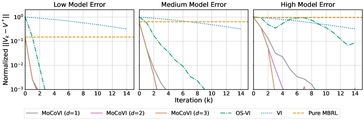
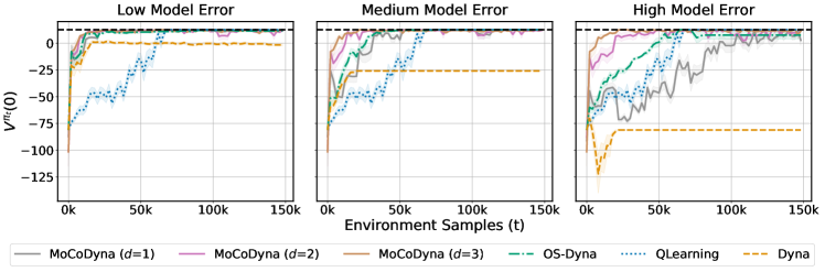
Figure 1: Comparison of (top) MoCoVI with VI, pure MBRL and OS-VI, and (bottom) MoCoDyna with QLearning, Dyna, and OS-Dyna. (Left) low ($\lambda=0.1$), (Middle) medium ($\lambda=0.5$), and (Right) high ($\lambda=1$) model errors. Each curve is average of 20 runs. Shaded areas show the standard error.

We empirically show the effectiveness of MoCoVI and MoCoDyna to utilize an approximate model. We consider the $6\times 6$ grid world environment with four actions introduced by Rakhsha et al. (2022), with $\gamma=0.9$. We defer the details of the environment to the supplementary material. As shown in Theorem 2, the convergence rate of MoCoVI depends on the model error and $d$. We introduce error to $\hat{\mathcal{P}}$ by smoothing the true dynamics $\mathcal{P}$ as suggested by Rakhsha et al. (2022): for $\lambda\in[0,1]$, the smoothed dynamics $\mathcal{P}^{(\lambda)}$ is $\mathcal{P}^{(\lambda)}(\cdot|x,a)\triangleq(1-\lambda)\cdot\mathcal{P}(\cdot|x,a)+\lambda\cdot U\big{(}\{x^{\prime}|\mathcal{P}(x^{\prime}|x,a)>0\}\big{)}$, where $U(S)$ is the uniform distribution over set $S$. The parameter $\lambda$ controls the model error, from no error with $\lambda=0$ to a large error with $\lambda=1$ (uniform transition probability over possible next-states).

Fig.  1 first compares MoCoVI with OS-VI (Rakhsha et al., 2022), VI, and the value function obtained based on the model. We set $\hat{\mathcal{P}}=\mathcal{P}^{(\lambda)}$ for $\lambda=0.1,0.5$ and $1$. The plot shows normalized error of $V_{k}$ against $V^{*}$, that is, $\|V_{k}-V^{*}\|_{1}/\|V^{*}\|_{1}$. MoCoVI can converge to the true value function in a few iterations even with extreme model errors. The robustness, as expected, is improved with larger values of $d$. In comparison, OS-VI and VI show a much slower rate than MoCoVI and the value function obtained from $\hat{\mathcal{P}}$ suffers from the model error. Fig. 1 then shows the results in the RL setting. We compare MoCoDyna with OS-Dyna (Rakhsha et al., 2022), QLearning, and Dyna. At each step, the algorithms are given a sample $(X_{t},A_{t},R_{t},X_{t}^{\prime})$ where $X_{t},A_{t}$ are chosen uniformly in random. We use $\hat{\mathcal{P}}=\mathcal{P}^{(\lambda)}_{\mathrm{MLE}}$ where $\mathcal{P}_{\mathrm{MLE}}$ is the MLE estimate of dynamics at the moment. For OS-Dyna and QLearning which have a learning rate, for some $\alpha,N>0$, we use the constant learning $\alpha$ for $t\leq N$ and $\alpha/(t-N)$ for $t>N$ to allow both fast initial convergence and stability. The results show a similar pattern as for MoCoVI. MoCoDyna can successfully solve the task with any model error. In fact, MoCo with $d=2,3$ significantly outperforms other algorithms. In comparison, QLearning and OS-Dyna show a slower rate of convergence, and Dyna cannot solve the task due to the model error.

7 Conclusion

In this work, we set out to bridge model-based and model-free approaches in RL by devising a cost-efficient approach to alleviate model errors. We develop the MaxEnt model correction framework, which adopts MaxEnt density estimation to reduce model errors given a small number of queries to the true dynamics. A thorough theoretical analysis indicates that our framework can significantly accelerate the convergence rate of policy evaluation and control algorithms, and ensure convergence to the true value functions despite model errors if said errors are sufficiently small. We also develop a sample-based variant, MoCoDyna, which extends the Dyna framework. Lastly, we confirm the practical relevance of our theoretical findings by benchmarking MoCo-based planning algorithms against their naive counterparts, and showing superior performance both in terms of convergence rate and expected returns. Future work should investigate deep RL applications of the MoCo framework.

Acknowledgments

We would like to thank the members of the Adaptive Agents Lab, especially Claas Voelcker, who provided feedback on a draft of this paper. AMF acknowledges the funding from the Canada CIFAR AI Chairs program, as well as the support of the Natural Sciences and Engineering Research Council of Canada (NSERC) through the Discovery Grant program (2021-03701). MK acknowledges the support of NSERC via the Canada Graduate Scholarship - Doctoral program (CGSD3-568998-2022). Resources used in preparing this research were provided, in part, by the Province of Ontario, the Government of Canada through CIFAR, and companies sponsoring the Vector Institute.

Appendix A List of appendices

• Appendix B provides extended background on MDPs.

• Appendix C contains the proofs for Section 2.1.

• Appendix D provides technical details of Maximum Entropy Density Estimation.

• Appendix E contains the proofs for Section 3.1.

• Appendix F contains the proofs for Section 3.2.

• Appendix G provides the analysis of MaxEnt MoCo in $\ell_{p}$ norms.

• Appendix H contains the proofs for $\ell_{p}$ analysis of MaxEnt MoCo.

• Appendix I contains the proofs for Section 4.

• Appendix J shows additional empirical results.

Appendix B Background on Markov Decision Processes

In this work, we consider a discounted Markov Decision Process (MDP) defined as ${M=({\mathcal{X}},{\mathcal{A}},\mathcal{R},\mathcal{P},\gamma)}$ [Bertsekas and Tsitsiklis, 1996, Szepesvári, 2010, Sutton and Barto, 2019]. Here, ${\mathcal{X}}$ is the state space, ${\mathcal{A}}$ is the action space, $\mathcal{R}\colon{\mathcal{X}}\times{\mathcal{A}}\to\mathcal{M}(\mathbb{R})$ is the reward kernel, $\mathcal{P}\colon{\mathcal{X}}\times{\mathcal{A}}\to\mathcal{M}({\mathcal{X}})$ is the transition kernel, and $0\leq\gamma<1$ is the discount factor. We define $r\colon{\mathcal{X}}\times{\mathcal{A}}\to\mathbb{R}$ to be the expected reward and assume it is known to the agent. A policy $\pi\colon{\mathcal{X}}\to\mathcal{M}({\mathcal{A}})$ is a mapping from states to distributions over actions. We denote the expected rewards and transitions of a policy $\pi$ by $r^{\pi}\colon{\mathcal{X}}\to\mathbb{R}$ and $\mathcal{P}^{\pi}\colon{\mathcal{X}}\to\mathcal{M}({\mathcal{X}})$, respectively. For any function $\phi\colon{\mathcal{X}}\to\mathbb{R}$, we define $\mathcal{P}\phi\colon{\mathcal{X}}\times{\mathcal{A}}\to\mathbb{R}$ as

$$(\mathcal{P}\phi)(x,a)\triangleq\int\mathcal{P}(\mathrm{d}x^{\prime}|x,a)\phi(x^{\prime})\qquad(\forall x,a).$$

The value function ${V^{\pi}=V^{\pi}(\mathcal{R},\mathcal{P})}$ of a policy $\pi$ is defined as

$${V^{\pi}(x)\triangleq\mathbb{E}\mathopen{}\mathclose{{}\left[{\sum_{t=0}^{\infty}\gamma^{t}R_{t}|X_{0}=x}}\right]},$$

where actions are taken according to $\pi$, and $X_{t}$ and $R_{t}$ are the state and reward at step $t$. The value function of $\pi$ satisfies the Bellman equation: For all $x\in{\mathcal{X}}$, we have

$$V^{\pi}(x)=r^{\pi}(x)+\gamma\int\mathcal{P}^{\pi}(\mathrm{d}x^{\prime}|x)V^{\pi}(x^{\prime}),$$ (B.1)

or in short, $V^{\pi}=r^{\pi}+\gamma\mathcal{P}^{\pi}V^{\pi}$. The optimal value function $V^{*}=V^{*}(\mathcal{R},\mathcal{P})$ is defined such that ${V^{*}(x)=\max_{\pi}V^{\pi}(x)}$ for all states $x\in{\mathcal{X}}$. Similarly, $V^{*}$ satisfies the Bellman optimality equation:

$$V^{*}(x)=\max_{a\in{\mathcal{A}}}~{}\mathopen{}\mathclose{{}\left\{r(x,a)+\gamma\int\mathcal{P}(\mathrm{d}x^{\prime}|x,a)V^{*}(x^{\prime})}\right\}.$$ (B.2)

We denote an optimal policy by $\pi^{*}=\pi^{*}(\mathcal{P},\mathcal{R})$, for which we have $V^{*}=V^{\pi^{*}}$. We refer to the problem of finding $V^{\pi_{\text{PE}}}$ for a specific policy ${\pi_{\text{PE}}}$ as the Policy Evaluation (PE) problem, and to the problem of finding an optimal policy as the Control problem.

The greedy policy at state $x\in{\mathcal{X}}$ is

$${\pi}_{g}(x;V)\leftarrow\mathop{\mathrm{missing}}{argmax}_{a\in{\mathcal{A}}}\mathopen{}\mathclose{{}\left\{r(x,a)+\gamma\int\mathcal{P}(\mathrm{d}y|x,a)V(y)}\right\}.$$ (B.3)

In this paper, we assume an approximate model $\hat{\mathcal{P}}\approx\mathcal{P}$ is given. We define $\hat{V}^{\pi}$ and $\hat{\pi}^{*}$ in the approximate MDP $\hat{M}=({\mathcal{X}},{\mathcal{A}},\mathcal{R},\hat{\mathcal{P}},\gamma)$ similar to their counterparts in the true MDP $M$.

Appendix C Proofs for Section 2.1

In this section, we provide the proof of Lemma 1. Before that, we first show two useful lemmas.

Lemma 2.

For two transition dynamics $\mathcal{P}_{1},\mathcal{P}_{2}$ and any policy $\pi$ we have

$$\mathopen{}\mathclose{{}\left\|{\mathcal{P}_{1}^{\pi}(\cdot|x)-\mathcal{P}_{2}^{\pi}(\cdot|x)}}\right\|_{1}\leq\sqrt{2}\int\pi(\mathrm{d}a|x)\sqrt{D_{\textnormal{KL}}(\;{\mathcal{P}_{1}(\cdot|x,a)}\;\|\;{\mathcal{P}_{2}(\cdot|x,a)}\;)}$$

Proof.  We have

$$\mathopen{}\mathclose{{}\left\|{\mathcal{P}_{1}^{\pi}(\cdot|x)-\mathcal{P}_{2}^{\pi}(\cdot|x)}}\right\|_{1} =\int_{y}\mathopen{}\mathclose{{}\left|\mathcal{P}_{1}^{\pi}(\mathrm{d}y|x)-\mathcal{P}_{2}^{\pi}(\mathrm{d}y|x)}\right|$$

$$=\int_{y}\mathopen{}\mathclose{{}\left|\int_{a}\pi(\mathrm{d}a,x)(\mathcal{P}_{1}(\mathrm{d}y|x,a)-\mathcal{P}_{2}(\mathrm{d}y|x,a))}\right|$$

$$\leq\int_{y}\int_{a}\pi(\mathrm{d}a,x)\mathopen{}\mathclose{{}\left|\mathcal{P}_{1}(\mathrm{d}y|x,a)-\mathcal{P}_{2}(\mathrm{d}y|x,a)}\right|$$

$$=\int_{a}\pi(\mathrm{d}a,x)\int_{y}\mathopen{}\mathclose{{}\left|\mathcal{P}_{1}(\mathrm{d}y|x,a)-\mathcal{P}_{2}(\mathrm{d}y|x,a)}\right|$$

$$=\int_{a}\pi(\mathrm{d}a,x)\mathopen{}\mathclose{{}\left\|{\mathcal{P}_{1}(\cdot|x,a)-\mathcal{P}_{2}(\cdot|x,a)}}\right\|_{1}$$ (C.1)

$$\leq\int_{a}\pi(\mathrm{d}a,x)\sqrt{2D_{\textnormal{KL}}(\;{\mathcal{P}_{1}(\cdot|x,a)}\;\|\;{\mathcal{P}_{2}(\cdot|x,a)}\;)}$$

where we used the Pinsker’s inequality. ∎

Lemma 3.

For two transition dynamics $\mathcal{P}_{1},\mathcal{P}_{2}$ and any policy $\pi$, Define

$$G^{\pi}_{\mathcal{P}_{1},\mathcal{P}_{2}}\triangleq(\mathbf{I}-\gamma\mathcal{P}^{\pi}_{2})^{-1}(\gamma\mathcal{P}^{\pi}_{1}-\mathcal{P}^{\pi}_{2})$$

We have

$$\mathopen{}\mathclose{{}\left\|{G^{\pi}_{\mathcal{P}^{\pi}_{1},\mathcal{P}^{\pi}_{2}}}}\right\|_{\infty}\leq\frac{\gamma\sqrt{2}}{1-\gamma}\sup_{x,a}\sqrt{D_{\textnormal{KL}}(\;{\mathcal{P}_{1}(\cdot|x,a)}\;\|\;{\mathcal{P}_{2}(\cdot|x,a)}\;)}$$

Proof.  When clear from context, we write $G^{\pi}$ instead of $G^{\pi}_{\mathcal{P}_{1},\mathcal{P}_{2}}$. We have

$$\mathopen{}\mathclose{{}\left\|{G^{\pi}}}\right\|_{\infty} \leq\gamma\mathopen{}\mathclose{{}\left\|{(\mathbf{I}-\gamma\mathcal{P}^{\pi}_{2})^{-1}}}\right\|_{\infty}\mathopen{}\mathclose{{}\left\|{\mathcal{P}^{\pi}_{1}-\mathcal{P}^{\pi}_{2}}}\right\|_{\infty}$$

$$\leq\frac{\gamma}{1-\gamma}\sup_{x}\mathopen{}\mathclose{{}\left\|{\mathcal{P}^{\pi}_{1}(\cdot|x)-\mathcal{P}^{\pi}_{2}(\cdot|x)}}\right\|_{1}$$

where we used $\mathopen{}\mathclose{{}\left\|{(\mathbf{I}-A)^{-1}=1/(1-\mathopen{}\mathclose{{}\left\|{A}}\right\|_{\infty})}}\right\|_{\infty}$ for $\mathopen{}\mathclose{{}\left\|{A}}\right\|_{\infty}\leq 1$ and the fact that $\mathopen{}\mathclose{{}\left\|{\mathcal{P}^{\pi}_{2}}}\right\|_{\infty}=1$. Due to Lemma 2 we have for any $x$

$$\mathopen{}\mathclose{{}\left\|{\mathcal{P}^{\pi}_{1}(\cdot|x)-\mathcal{P}^{\pi}_{2}(\cdot|x)}}\right\|_{1} \leq\sqrt{2}\int\pi(\mathrm{d}a|x)\sqrt{D_{\textnormal{KL}}(\;{\mathcal{P}_{1}(\cdot|x,a)}\;\|\;{\mathcal{P}_{2}(\cdot|x,a)}\;)}$$

$$\leq\sup_{x,a}\sqrt{2D_{\textnormal{KL}}(\;{\mathcal{P}_{1}(\cdot|x,a)}\;\|\;{\mathcal{P}_{2}(\cdot|x,a)}\;)}$$

substituting this in the bound for $\mathopen{}\mathclose{{}\left\|{G^{\pi}}}\right\|_{\infty}$ gives the result. ∎

We now give the proof of Lemma 1.

Proof of Lemma 1 for PE

Proof.  Since $\hat{V}^{\pi}=(\mathbf{I}-\gamma\hat{\mathcal{P}}^{\pi})^{-1}r^{\pi}$ and $r^{\pi}=(\mathbf{I}-\gamma\mathcal{P}^{\pi})V^{\pi}$ we have

$$V^{\pi}-\hat{V}^{\pi} =(\mathbf{I}-\gamma\hat{\mathcal{P}}^{\pi})^{-1}(\mathbf{I}-\gamma\hat{\mathcal{P}}^{\pi})V^{\pi}-(\mathbf{I}-\gamma\hat{\mathcal{P}}^{\pi})^{-1}r^{\pi}$$

$$=(\mathbf{I}-\gamma\hat{\mathcal{P}}^{\pi})^{-1}[(\mathbf{I}-\gamma\hat{\mathcal{P}}^{\pi})V^{\pi}-(\mathbf{I}-\gamma\mathcal{P}^{\pi})V^{\pi}]$$

$$=(\mathbf{I}-\gamma\hat{\mathcal{P}}^{\pi})^{-1}(\gamma\mathcal{P}^{\pi}-\gamma\hat{\mathcal{P}}^{\pi})V^{\pi}$$

$$=G^{\pi}_{\mathcal{P},\hat{\mathcal{P}}}V^{\pi}$$ (C.2)

Thus,

$$\mathopen{}\mathclose{{}\left\|{V^{\pi}-\hat{V}^{\pi}}}\right\|_{\infty} \leq\gamma\mathopen{}\mathclose{{}\left\|{(\mathbf{I}-\gamma\hat{\mathcal{P}}^{\pi})^{-1}}}\right\|_{\infty}\mathopen{}\mathclose{{}\left\|{(\mathcal{P}^{\pi}-\hat{\mathcal{P}}^{\pi})V^{\pi}}}\right\|_{\infty}$$

$$\leq\frac{\gamma}{1-\gamma}\mathopen{}\mathclose{{}\left\|{(\mathcal{P}^{\pi}-\hat{\mathcal{P}}^{\pi})V^{\pi}}}\right\|_{\infty}$$

$$\leq\frac{\gamma}{1-\gamma}\mathopen{}\mathclose{{}\left\|{(\mathcal{P}^{\pi}-\hat{\mathcal{P}}^{\pi})}}\right\|_{\infty}\mathopen{}\mathclose{{}\left\|{V^{\pi}}}\right\|_{\infty}$$

$$\leq\frac{\gamma\sqrt{2}}{1-\gamma}\mathopen{}\mathclose{{}\left\|{\epsilon_{\mathrm{Model}}}}\right\|_{\infty}\mathopen{}\mathclose{{}\left\|{V^{\pi}}}\right\|_{\infty}$$

where we followed the proof of Lemma 3 for the last inequality. ∎

Proof of Lemma 1 for Control

Proof.  Define $r_{0}=r+(\gamma\mathcal{P}-\gamma\hat{\mathcal{P}})V^{*}$ similar to Rakhsha et al. [2022, Lemma 3]

$$V^{\pi^{*}}(r_{0},\hat{\mathcal{P}})=V^{*}(r,\mathcal{P}).$$

Assume $f\preccurlyeq g$ mean $f(x)\geq g(x)$ for any $x$. We can write

$$0 \preccurlyeq V^{\pi^{*}}(r,\mathcal{P})-V^{\hat{\pi}^{*}}(r,\mathcal{P})$$

$$=V^{\pi^{*}}(r_{0},\hat{\mathcal{P}})-V^{\hat{\pi}^{*}}(r,\mathcal{P})$$

$$=V^{\pi^{*}}(r_{0},\hat{\mathcal{P}})-V^{\pi^{*}}(r,\hat{\mathcal{P}})+V^{\pi^{*}}(r,\hat{\mathcal{P}})-V^{\hat{\pi}^{*}}(r,\mathcal{P})$$

$$\preccurlyeq V^{\pi^{*}}(r_{0},\hat{\mathcal{P}})-V^{\pi^{*}}(r,\hat{\mathcal{P}})+V^{\hat{\pi}^{*}}(r,\hat{\mathcal{P}})-V^{\hat{\pi}^{*}}(r,\mathcal{P})$$

$$=(\mathbf{I}-\gamma\hat{\mathcal{P}}^{\pi^{*}})^{-1}(r_{0}^{\pi^{*}}-r^{\pi^{*}})+V^{\hat{\pi}^{*}}(r,\hat{\mathcal{P}})-V^{\hat{\pi}^{*}}(r,\mathcal{P})$$

$$=(\mathbf{I}-\gamma\hat{\mathcal{P}}^{\pi^{*}})^{-1}(\gamma\mathcal{P}^{\pi^{*}}-\gamma\hat{\mathcal{P}}^{\pi^{*}})V^{*}+V^{\hat{\pi}^{*}}(r,\hat{\mathcal{P}})-V^{\hat{\pi}^{*}}(r,\mathcal{P})$$

$$=G^{\pi^{*}}_{\mathcal{P},\hat{\mathcal{P}}}V^{*}+V^{\hat{\pi}^{*}}(r,\hat{\mathcal{P}})-V^{\hat{\pi}^{*}}(r,\mathcal{P})$$

$$=G^{\pi^{*}}_{\mathcal{P},\hat{\mathcal{P}}}V^{*}-G^{\hat{\pi}^{*}}_{\mathcal{P},\hat{\mathcal{P}}}V^{\hat{\pi}^{*}}(r,\mathcal{P})$$

$$=G^{\pi^{*}}_{\mathcal{P},\hat{\mathcal{P}}}V^{*}-G^{\hat{\pi}^{*}}_{\mathcal{P},\hat{\mathcal{P}}}V^{*}+G^{\hat{\pi}^{*}}_{\mathcal{P},\hat{\mathcal{P}}}(V^{*}-V^{\hat{\pi}^{*}}(r,\mathcal{P}))$$

$$\preccurlyeq\mathopen{}\mathclose{{}\left|G^{\pi^{*}}_{\mathcal{P},\hat{\mathcal{P}}}V^{*}}\right|+\mathopen{}\mathclose{{}\left|G^{\hat{\pi}^{*}}_{\mathcal{P},\hat{\mathcal{P}}}V^{*}}\right|+\mathopen{}\mathclose{{}\left|G^{\hat{\pi}^{*}}_{\mathcal{P},\hat{\mathcal{P}}}(V^{*}-V^{\hat{\pi}^{*}}(r,\mathcal{P}))}\right|$$

where we used (C.2). Comparing the first line with the least, we obtain

$$\mathopen{}\mathclose{{}\left\|{V^{\pi^{*}}-V^{\hat{\pi}^{*}}}}\right\|_{\infty} \leq\mathopen{}\mathclose{{}\left\|{G^{\pi^{*}}_{\mathcal{P},\hat{\mathcal{P}}}V^{*}}}\right\|_{\infty}+\mathopen{}\mathclose{{}\left\|{G^{\hat{\pi}^{*}}_{\mathcal{P},\hat{\mathcal{P}}}V^{*}}}\right\|_{\infty}+\mathopen{}\mathclose{{}\left\|{G^{\hat{\pi}^{*}}_{\mathcal{P},\hat{\mathcal{P}}}(V^{*}-V^{\hat{\pi}^{*}})}}\right\|_{\infty}$$ (C.3)

$$\leq 2c_{1}\mathopen{}\mathclose{{}\left\|{\epsilon_{\mathrm{Model}}}}\right\|_{\infty}\mathopen{}\mathclose{{}\left\|{V^{*}}}\right\|_{\infty}++c_{1}\mathopen{}\mathclose{{}\left\|{\epsilon_{\mathrm{Model}}}}\right\|_{\infty}\mathopen{}\mathclose{{}\left\|{V^{*}-V^{\hat{\pi}^{*}}}}\right\|_{\infty}$$

where we used Lemma 3. Rearranging the terms give the result. ∎

Appendix D Technical details of Maximum Entropy Density Estimation

In this section we present the technical details of maximum entropy density estimation. This involves the duality methods for solving the optimization algorithms and some useful lemmas regarding their solutions. These problems are well studied in the literature. We do not make any assumptions on whether the environment states space, which will be the domain of the distributions in this section, is finite or continuous, and we make arguments for general measures. Due to this, our assumptions as well as our constraints may differ from the original papers in the literature. In those cases, we prove the results ourselves.

D.1 Maximum Entropy Density Estimation with Equality Constraints

Assume $Z$ is a random variable over domain ${\mathcal{Z}}$ with an unknown distribution $p\in\mathcal{M}({\mathcal{Z}})$. For a set of functions $\phi_{1},\ldots,\phi_{d}\colon{\mathcal{Z}}\to\mathbb{R}$ the expected values $\bar{\phi}_{i}=\mathbb{E}_{Z\sim p}\mathopen{}\mathclose{{}\left[{\phi_{i}(Z)}}\right]$ are given. We will use ${\boldsymbol{\phi}}\colon{\mathcal{Z}}\to\mathbb{R}^{d}$ and $\bar{\boldsymbol{\phi}}\in\mathbb{R}^{d}$ to refer to the respective vector forms. We also have access to an approximate distribution $\hat{p}\in\mathcal{M}({\mathcal{Z}})$ such that $\hat{p}\approx p$. The maximum entropy density estimation gives a new approximation $q^{*}$ that is the solution of the following optimization problem

$$\min_{q\in\mathcal{M}({\mathcal{Z}})} \;\;D_{\textnormal{KL}}(\;{q}\;\|\;{\hat{p}}\;),$$ (D.1)

s.t. $$\;\;\mathbb{E}_{Z\sim q}\mathopen{}\mathclose{{}\left[{\phi_{i}(Z)}}\right]=\bar{\phi}_{i}\qquad(1\leq i\leq d).$$

The KL-divergence in (D.1) is finite only if $q$ is absolutely continuous w.r.t. $\hat{p}$. In that case, $q$ can be specified with its density w.r.t $\hat{p}$ defined as $f\triangleq\frac{\mathrm{d}q}{\mathrm{d}\hat{p}}\colon{\mathcal{Z}}\to\mathbb{R}$ where $\frac{\mathrm{d}q}{\mathrm{d}\hat{p}}$ is the Radon-Nikodym derivative. Let $L_{1}({\mathcal{Z}},\hat{p})$ be the $L_{1}$ space over ${\mathcal{Z}}$ with measure $\hat{p}$. We have $f\in L_{1}({\mathcal{Z}},\hat{p})$.

Also for any $f\in L_{1}({\mathcal{Z}},\hat{p})$ such that $f\geq 0$ and $\int f(z)\hat{p}(\mathrm{d}z)=1$ we can recover a distribution $q\in\mathcal{M}({\mathcal{Z}})$ as

$$q(A)=\int_{A}f(z)\hat{p}(\mathrm{d}z).$$ (D.2)

Consequently, (D.1) can be written in terms of $f$. We have

$$D_{\textnormal{KL}}(\;{q}\;\|\;{\hat{p}}\;) =\int q(\mathrm{d}z)\log\frac{q(\mathrm{d}z)}{p(\mathrm{d}z)}$$

$$=\int\frac{q(\mathrm{d}z)}{p(\mathrm{d}z)}\log\frac{q(\mathrm{d}z)}{p(\mathrm{d}z)}\cdot\hat{p}(\mathrm{d}z)$$

$$=\int f(z)\log f(z)\cdot\hat{p}(\mathrm{d}z)$$

We can write (D.1) as

$$\min_{f} \;\;\int f(z)\log f(z)\;\hat{p}(\mathrm{d}z),$$ (D.3)

s.t. $$\;\;\int f(z)\phi_{i}(z)\;\hat{p}(\mathrm{d}z)=\bar{\phi}_{i}\qquad(1\leq i\leq d),$$

$$\;\;\int f(z)\;\hat{p}(\mathrm{d}z)=1,$$

$$\;\;f\in L_{1}({\mathcal{Z}},\hat{p}).$$

The constraint $f\geq 0$ is implicit in the domain of the KL objective. The Lagrangian with dual parameters $\lambda,\Lambda^{\prime}$ is

$$L(f,\lambda,\Lambda^{\prime})=\int\mathopen{}\mathclose{{}\left[f(z)\log f(z)-\sum_{i=1}^{d}\lambda_{i}f(z)\phi_{i}(z)+\Lambda^{\prime}f(z)}\right]\;\hat{p}(\mathrm{d}z)+\sum_{i}\lambda_{i}\bar{\phi}_{i}-\Lambda^{\prime}.$$ (D.4)

Then, we can obtain the dual objective $D_{\bar{\boldsymbol{\phi}}}(\lambda,\Lambda^{\prime})\triangleq\inf_{f}L(f,\lambda,\Lambda^{\prime})$ from this result by Decarreau et al. [1992, Proposition 2.4].

Lemma 4 ([Decarreau et al., 1992]).

For any fixed $\lambda\in\mathbb{R}^{d},\Lambda^{\prime}\in\mathbb{R}$, the Lagrangian $L$ in (D.4) has a unique minimizer $f_{\lambda,\Lambda^{\prime}}$ defined as

$$f_{\lambda,\Lambda^{\prime}}\triangleq\operatorname{exp}\bigg{(}\sum_{i=1}^{d}\lambda_{i}\phi_{i}(z)-\Lambda^{\prime}-1\bigg{)}.$$

The dual objective is given by

$$D_{\bar{\boldsymbol{\phi}}}(\lambda,\Lambda^{\prime})=-\int\operatorname{exp}\bigg{(}\sum_{i=1}^{d}\lambda_{i}\phi_{i}(z)-\Lambda^{\prime}-1\bigg{)}\hat{p}(\mathrm{d}z)+\sum_{i=1}^{d}\lambda_{i}\bar{\phi}_{i}-\Lambda^{\prime}.$$

It is concave, continuously differentiable, and its partial derivatives are

$$\frac{\partial D_{\bar{\boldsymbol{\phi}}}(\lambda,\Lambda^{\prime})}{\partial\lambda_{i}}=\bar{\phi}_{i}-\int f_{\lambda,\Lambda^{\prime}}(z)\phi_{i}(z)\hat{p}(\mathrm{d}z)\qquad,\qquad\frac{\partial D_{\bar{\boldsymbol{\phi}}}(\lambda,\Lambda^{\prime})}{\partial\Lambda^{\prime}}=1-\int f_{\lambda,\Lambda^{\prime}}(z)\hat{p}(\mathrm{d}z).$$

Thus, for the dual objective $D_{\bar{\boldsymbol{\phi}}}(\lambda,\Lambda^{\prime})$ we have $D_{\bar{\boldsymbol{\phi}}}(\lambda,\Lambda^{\prime})=L(f_{\lambda,\Lambda^{\prime}},\lambda,\Lambda^{\prime})$. We arrive at the following dual problem

$$\max_{\lambda\in\mathbb{R}^{d},\Lambda^{\prime}\in\mathbb{R}}D_{\bar{\boldsymbol{\phi}}}(\lambda,\Lambda^{\prime})=\mathopen{}\mathclose{{}\left[-\int\operatorname{exp}\bigg{(}\sum_{i=1}^{d}\lambda_{i}\phi_{i}(z)-\Lambda^{\prime}-1\bigg{)}\hat{p}(\mathrm{d}z)+\sum_{i=1}^{d}\lambda_{i}\bar{\phi}_{i}-\Lambda^{\prime}}\right],$$ (D.5)

The following result by Borwein and Lewis [1991, Corollary 2.6 and Theorem 4.8] shows the duality of the problems.

Theorem 3 ([Borwein and Lewis, 1991]).

Assume $\phi_{i}\in L_{\infty}({\mathcal{Z}},\hat{p})$ for $i=1,\ldots,n$. Under certain constraint qualification constraints, the value of (D.3) and (D.5) is equal with dual attainment. Furthermore, let $\lambda^{*},\Lambda^{\prime*}$ be dual optimal. The primal optimal solution is $f_{\lambda^{*},\Lambda^{\prime*}}$.

We do not discuss the technical details of the constraint qualification constraints and refer the readers to [Altun and Smola, 2006, Borwein and Lewis, 1991, Decarreau et al., 1992] for a complete discussion.

For any $\lambda\in\mathbb{R}^{d}$, the optimal value of $\Lambda^{\prime}$ can be computed. Due to Lemma 4, we have

$$\frac{\partial D_{\bar{\boldsymbol{\phi}}}(\lambda,\Lambda^{\prime})}{\partial\Lambda^{\prime}}=\frac{\partial D_{\beta,\bar{\boldsymbol{\phi}}}(\lambda,\Lambda^{\prime})}{\partial\Lambda^{\prime}}=1-\int f_{\lambda,\Lambda^{\prime}}(z)\hat{p}(\mathrm{d}z)$$ (D.6)

solving for the optimal $\Lambda^{\prime}$ gives the following value

$$\Lambda^{\prime}_{\lambda}\triangleq\log\int\operatorname{exp}\bigg{(}\sum_{i=1}^{d}\lambda_{i}\phi_{i}(z)-1\bigg{)}\hat{p}(\mathrm{d}z)=\Lambda_{\lambda}-1,$$ (D.7)

where $\Lambda_{\lambda}$ is defined in Section 2.2. Note that since functions $\phi_{i}$ are bounded this quantity is finite. Thus, we can just optimize $D_{\bar{\boldsymbol{\phi}}}(\lambda,\Lambda^{\prime}_{\lambda})$ over $\lambda$. By substitution we get

$$D_{\bar{\boldsymbol{\phi}}}(\lambda)\triangleq D_{\bar{\boldsymbol{\phi}}}(\lambda,\Lambda^{\prime}_{\lambda})=\sum_{i=1}^{d}\lambda_{i}\bar{\phi}_{i}-\log\int\operatorname{exp}\bigg{(}\sum_{i=1}^{d}\lambda_{i}\phi_{i}(z)\bigg{)}\hat{p}(\mathrm{d}z).$$ (D.8)

We observe that $\max_{\lambda}D_{\bar{\boldsymbol{\phi}}}(\lambda)$ is equivalent to (2.4). From Theorem 3, if $\lambda^{*}$ optimizes $D_{\bar{\boldsymbol{\phi}}}$, we know that $f_{\lambda^{*},\Lambda^{\prime}_{\lambda^{*}}}$ optimizes (D.3). Due to equivalence of (D.3) and (D.1), then $q_{\lambda^{*}}$ defined as

$$q_{\lambda^{*}}(A)\triangleq\int_{A}f_{\lambda^{*},\Lambda^{\prime}_{\lambda^{*}}}(z)\hat{p}(\mathrm{d}z)=\int_{z\in A}\hat{p}(\mathrm{d}z)\cdot\operatorname{exp}\mathopen{}\mathclose{{}\left(\sum_{i=1}^{d}\lambda_{i}^{*}\phi_{i}(z)-\Lambda_{\lambda^{*}}}\right)$$ (D.9)

for all $A\subseteq{\mathcal{Z}}$ optimizes (D.1).

D.2 Maximum Entropy Density Estimation with $\ell_{2}^{2}$ Regularization

We now study a relaxed form of the maximum entropy density estimation. In this form, instead of imposing strict equality constraints, the mismatch between the expected value $\mathbb{E}_{Z\sim q}\mathopen{}\mathclose{{}\left[{\phi_{i}(Z)}}\right]$ with $\bar{\phi}_{i}$ is added to the loss. The benefit of this version is that even if $\bar{\phi}_{i}$ values are not exactly equal to $\mathbb{E}_{Z\sim p}\mathopen{}\mathclose{{}\left[{\phi_{i}(Z)}}\right]$, the problem remains feasible. Moreover, we can adjust the weight of this term in the loss based on the accuracy of $\bar{\phi}_{i}$ values. Specifically, we define the following problem.

$$\min_{q\in\mathcal{M}({\mathcal{Z}})} \;\;D_{\textnormal{KL}}(\;{q}\;\|\;{\hat{p}}\;)+\frac{1}{\beta^{2}}\sum_{i=1}^{d}\Big{(}\mathbb{E}_{Z\sim q}\mathopen{}\mathclose{{}\left[{\phi_{i}(Z)}}\right]-\bar{\phi}_{i}\Big{)}^{2}$$ (D.10)

Similar to the previous section, we can write the above problem in terms of the density $\frac{\mathrm{d}q}{\mathrm{d}\hat{p}}$ and write [Decarreau et al., 1992]

$$\min_{f,\xi} \;\;\int f(z)\log f(z)\;\hat{p}(\mathrm{d}z)+\frac{1}{\beta^{2}}\sum_{i=1}^{d}\xi_{i}^{2},$$ (D.11)

s.t. $$\;\;\int f(z)\phi_{i}(z)\;\hat{p}(\mathrm{d}z)-\bar{\phi}_{i}=\xi_{i}\qquad(1\leq i\leq d),$$

$$\;\;\int f(z)\;\hat{p}(\mathrm{d}z)=1,$$

$$\;\;f\in L_{1}({\mathcal{Z}},\hat{p})\;,\;\xi\in\mathbb{R}^{d}.$$

The Lagrangian of this problems can be written as

$$L_{\beta}(f,\xi,\lambda,\Lambda^{\prime})=L(f,\lambda,\Lambda^{\prime})+\frac{1}{\beta^{2}}\sum_{i=1}^{d}\xi_{i}^{2}+\sum_{i=1}^{d}\lambda_{i}\xi_{i}$$ (D.12)

The dual objective is then

$$D_{\beta,\bar{\boldsymbol{\phi}}}(\lambda,\Lambda^{\prime})=\inf_{f,\xi}L_{\beta}(f,\xi,\lambda,\Lambda^{\prime})$$

It can be observed that $f$ and $\xi$ can be independently optimized for any fixed $\lambda,\Lambda^{\prime}$. Due to Lemma 4, the optimal value of $f$ is $f_{\lambda,\Lambda^{\prime}}$. The optimal value of $\xi_{i}$ can be calculated as

$$\xi_{\lambda}=-\frac{1}{2}\beta^{2}\lambda$$ (D.13)

We arrive at the following dual objective

$$D_{\beta,\bar{\boldsymbol{\phi}}}(\lambda,\Lambda^{\prime}) =L(f_{\lambda,\Lambda^{\prime}},\lambda,\Lambda^{\prime})+\frac{1}{4}\beta^{2}\sum_{i=1}^{d}\lambda_{i}^{2}+\frac{1}{\beta^{2}}\sum_{i=1}^{d}{\xi_{\lambda}}_{i}^{2}+\sum_{i=1}^{d}\lambda_{i}{\xi_{\lambda}}_{i},$$ (D.14)

$$=L(f_{\lambda,\Lambda^{\prime}},\lambda,\Lambda^{\prime})+\frac{1}{4}\beta^{2}\sum_{i=1}^{d}\lambda_{i}^{2}-\frac{1}{2}\beta^{2}\sum_{i=1}^{d}\lambda_{i}^{2},$$

$$=D_{\bar{\boldsymbol{\phi}}}(\lambda,\Lambda^{\prime})-\frac{1}{4}\beta^{2}\sum_{i=1}^{d}\lambda_{i}^{2},$$

which means we have the dual problem

$$\max_{\lambda\in\mathbb{R}^{d},\Lambda^{\prime}\in\mathbb{R}}D_{\bar{\boldsymbol{\phi}}}(\lambda,\Lambda^{\prime})-\frac{1}{4}\beta^{2}\sum_{i=1}^{d}\lambda_{i}^{2}.$$ (D2)

We now show the duality of the problems. Notice how this problem has an extra $\frac{1}{4}\beta^{2}\sum_{i=1}^{d}\lambda_{i}^{2}$ compared to (2.4). This is the reason this problem is considered the regularized version of (2.4). Notice that the regularization term also makes the dual loss strongly concave. This makes solving the optimization problem easier.

Theorem 4.

Assume $\phi_{i}$ is bounded for $i=1,\ldots,n$ and $\beta>0$. The value of (D.11) and (D2) is equal with dual attainment. Furthermore, let $\lambda^{*},\Lambda^{\prime*}$ be dual optimal. The primal optimal solution is $f_{\lambda^{*},\Lambda^{\prime*}}$.

Proof.  First, we show that the some solution $\lambda^{*},\Lambda^{\prime*}$ exists for the dual problem. To see this, first note that for any $\lambda\in\mathbb{R}^{d}$, the optimal value of $\Lambda^{\prime}$ is $\Lambda^{\prime}_{\lambda}$ defined in (D.6). Now we need to show $D_{\beta,\bar{\boldsymbol{\phi}}}(\lambda,\Lambda^{\prime}_{\lambda})$ is maximized by some $\lambda^{*}$. We have

$$D_{\beta,\bar{\boldsymbol{\phi}}}(\lambda,\Lambda^{\prime}_{\lambda}) =D_{\bar{\boldsymbol{\phi}}}(\lambda,\Lambda^{\prime}_{\lambda})-\frac{1}{4}\beta^{2}\sum_{i=1}^{d}\lambda_{i}^{2}.$$ (D.15)

Since $D$ is concave, $D_{\bar{\boldsymbol{\phi}}}(\lambda,\Lambda^{\prime}_{\lambda})$ and therefore $D_{\beta,\bar{\boldsymbol{\phi}}}(\lambda,\Lambda^{\prime}_{\lambda})$ is also concave. Due to Weierstrass’ Theorem [Bertsekas, 2009, Proposition 3.2.1] it suffices to show the set

$$S=\{\;\lambda\in\mathbb{R}^{d}:D_{\beta,\bar{\boldsymbol{\phi}}}(\lambda,\Lambda^{\prime}_{\lambda})\geq D_{\beta,\bar{\boldsymbol{\phi}}}(0,\Lambda^{\prime}_{0})\;\}$$

is non-empty and bounded. It is trivially non-empty. Assume $|\phi(z)|\leq\phi_{\text{max}}$ for any $z$ and $1\leq i\leq d$. For any $\lambda\in S$, we have

$$D_{\beta,\bar{\boldsymbol{\phi}}}(0,\Lambda^{\prime}_{0}) \leq D_{\beta,\bar{\boldsymbol{\phi}}}(\lambda,\Lambda^{\prime}_{\lambda})$$

$$=D_{\bar{\boldsymbol{\phi}}}(\lambda,\Lambda^{\prime}_{\lambda})-\frac{1}{4}\beta^{2}\sum_{i=1}^{d}\lambda_{i}^{2}$$

$$=-\int\operatorname{exp}\bigg{(}\sum_{i=1}^{d}\lambda_{i}\phi_{i}(z)-\Lambda^{\prime}_{\lambda}-1\bigg{)}\hat{p}(\mathrm{d}z)+\sum_{i=1}^{d}\lambda_{i}\bar{\phi}_{i}-\Lambda^{\prime}_{\lambda}-\frac{1}{4}\beta^{2}\sum_{i=1}^{d}\lambda_{i}^{2}$$

$$=-1+\sum_{i=1}^{d}\lambda_{i}\bar{\phi}_{i}-\log\int\operatorname{exp}\bigg{(}\sum_{i=1}^{d}\lambda_{i}\phi_{i}(z)-1\bigg{)}\hat{p}(\mathrm{d}z)-\frac{1}{4}\beta^{2}\sum_{i=1}^{d}\lambda_{i}^{2}$$

$$\leq d\mathopen{}\mathclose{{}\left\|{\lambda}}\right\|_{\infty}\mathopen{}\mathclose{{}\left\|{\bar{\boldsymbol{\phi}}}}\right\|_{\infty}-\log\int\operatorname{exp}\bigg{(}-d\mathopen{}\mathclose{{}\left\|{\lambda}}\right\|_{\infty}\phi_{\text{max}}-1\bigg{)}\hat{p}(\mathrm{d}z)-\frac{1}{4}\beta^{2}\mathopen{}\mathclose{{}\left\|{\lambda}}\right\|_{\infty}^{2}$$

$$\leq-\frac{1}{4}\beta^{2}\mathopen{}\mathclose{{}\left\|{\lambda}}\right\|_{\infty}^{2}+d\mathopen{}\mathclose{{}\left\|{\lambda}}\right\|_{\infty}\mathopen{}\mathclose{{}\left\|{\bar{\boldsymbol{\phi}}}}\right\|_{\infty}+d\mathopen{}\mathclose{{}\left\|{\lambda}}\right\|_{\infty}\phi_{\text{max}}+1.$$

which enforces an upper bound on $\mathopen{}\mathclose{{}\left\|{\lambda}}\right\|_{\infty}$. This means that some optimal solution $\lambda^{*},\Lambda^{\prime}_{\lambda^{*}}$ exists.

Now we show that $f_{\lambda^{*},\Lambda^{\prime}_{\lambda^{*}}}$ is primal optimal with $\xi_{\lambda^{*}}$. First, note that the derivative (D.6) is zero for $\lambda^{*},\Lambda^{\prime}_{\lambda^{*}}$ due to the derivation of $\Lambda^{\prime}_{\lambda}$. Thus, $f_{\lambda^{*},\Lambda^{\prime}_{\lambda^{*}}}$ is feasible. Similarly using Lemma 4 we have from (D.15)

$$0 =\frac{\partial D_{\beta,\bar{\boldsymbol{\phi}}}(\lambda^{*},\Lambda^{\prime}_{\lambda^{*}})}{\partial\lambda_{i}}$$

$$=\frac{\partial D_{\bar{\boldsymbol{\phi}}}(\lambda^{*},\Lambda^{\prime}_{\lambda^{*}})}{\partial\lambda_{i}}-\frac{1}{2}\beta^{2}\lambda^{*}_{i}$$

$$=\bar{\phi}_{i}-\int f_{\lambda^{*},\Lambda^{\prime}_{\lambda^{*}}}(z)\phi_{i}(z)\hat{p}(\mathrm{d}z)+{\xi_{\lambda^{*}}}_{i},$$

which shows $\xi_{\lambda^{*}}$ is feasible.

Consider another feasible $f,\xi$ for (D.11).

$$\int f(z)\log f(z)\;\hat{p}(\mathrm{d}z)+\frac{1}{\beta^{2}}\sum_{i=1}^{d}\xi_{i}^{2} =L_{\beta}(f,\xi,\lambda^{*},\Lambda^{\prime}_{\lambda^{*}})$$

$$\geq D_{\beta,\bar{\boldsymbol{\phi}}}(\lambda^{*},\Lambda^{\prime}_{\lambda^{*}})$$

$$=L_{\beta}(f_{\lambda^{*},\Lambda^{\prime}_{\lambda^{*}}},\xi_{\lambda^{*}},\lambda^{*},\Lambda^{\prime}_{\lambda^{*}})$$

$$=\int f_{\lambda^{*},\Lambda^{\prime}_{\lambda^{*}}}(z)\log f_{\lambda^{*},\Lambda^{\prime}_{\lambda^{*}}}(z)\;\hat{p}(\mathrm{d}z)+\frac{1}{\beta^{2}}\sum_{i=1}^{d}{\xi_{\lambda^{*}}}^{2},$$

which proves the claim. ∎

Similar to the exact formulation, we can substitute $\Lambda^{\prime}$ with $\Lambda^{\prime}_{\lambda}$ to obtain a loss function based on $\lambda$. We arrive at the loss function

$$D_{\beta,\bar{\boldsymbol{\phi}}}(\lambda)\triangleq D_{\beta,\bar{\boldsymbol{\phi}}}(\lambda,\Lambda^{\prime}_{\lambda}) =D_{\bar{\boldsymbol{\phi}}}(\lambda,\Lambda^{\prime}_{\lambda})-\frac{1}{4}\beta^{2}\sum_{i=1}^{d}\lambda_{i}^{2}$$

$$=D_{\bar{\boldsymbol{\phi}}}(\lambda)-\frac{1}{4}\beta^{2}\sum_{i=1}^{d}\lambda_{i}^{2}$$

$$=\sum_{i=1}^{d}\lambda_{i}\bar{\phi}_{i}-\log\int\operatorname{exp}\bigg{(}\sum_{i=1}^{d}\lambda_{i}\phi_{i}(z)\bigg{)}\hat{p}(\mathrm{d}z)-\frac{1}{4}\beta^{2}\sum_{i=1}^{d}\lambda_{i}^{2}.$$ (D.16)

If $\lambda^{*}$ optimizes $D_{\beta,\bar{\boldsymbol{\phi}}}$, Theorem 4 shows $f_{\lambda^{*},\Lambda^{\prime}_{\lambda^{*}}}$ optimizes (D.11). Due to equivalence of (D.11) with (D.10), we get that $q_{\lambda^{*}}$ optimizes (D.10).

D.3 Lemmas Regarding Maximum Entropy Density Estimation

Lemma 5 (Dudík et al. [2007]).

For ${\boldsymbol{\phi}}^{(1)},{\boldsymbol{\phi}}^{(2)}\in\mathbb{R}^{d}$, let $\lambda^{(1)},\lambda^{(2)}$ be the maximizers of $D_{\beta,\bar{\boldsymbol{\phi}}^{(1)}}$ and $D_{\beta,\bar{\boldsymbol{\phi}}^{(2)}}$, respectively. We have

$$\mathopen{}\mathclose{{}\left\|{\lambda^{(1)}-\lambda^{(2)}}}\right\|_{2}\leq\frac{2}{\beta^{2}}\cdot\mathopen{}\mathclose{{}\left\|{\bar{\boldsymbol{\phi}}^{(1)}-\bar{\boldsymbol{\phi}}^{(2)}}}\right\|_{2}.$$

Proof.  Define

$$g(\lambda)\triangleq\log\int\operatorname{exp}\bigg{(}\sum_{i=1}^{d}\lambda_{i}\phi_{i}(z)\bigg{)}\hat{p}(\mathrm{d}z).$$

Since $g(\lambda)=\sum_{i=1}^{d}\lambda_{i}\bar{\phi}^{(1)}_{i}-D_{\bar{\boldsymbol{\phi}}^{(1)}}(\lambda)$ and $D_{\bar{\boldsymbol{\phi}}^{(1)}}(\lambda)$ is concave, we know that $g$ is convex. Due to optimality of $\lambda^{(1)},\lambda^{(2)}$ we have

$$\nabla D_{\beta,\bar{\boldsymbol{\phi}}^{(1)}}(\lambda^{(1)}) =-\nabla g(\lambda^{(1)})+\bar{\boldsymbol{\phi}}^{(1)}-\frac{1}{2}\beta^{2}\lambda^{(1)}=0,$$

$$\nabla D_{\beta,\bar{\boldsymbol{\phi}}^{(2)}}(\lambda^{(2)}) =-\nabla g(\lambda^{(2)})+\bar{\boldsymbol{\phi}}^{(2)}-\frac{1}{2}\beta^{2}\lambda^{(2)}=0.$$

By taking the difference we get

$$\frac{1}{2}\beta^{2}(\lambda^{(1)}-\lambda^{(2)})=-(\nabla g(\lambda^{(1)})-\nabla g(\lambda^{(2)}))+(\bar{\boldsymbol{\phi}}^{(1)}-\bar{\boldsymbol{\phi}}^{(2)}).$$

Multiplying both sides by $(\lambda^{(1)}-\lambda^{(2)})^{\top}$ we get

$$\frac{1}{2}\beta^{2}\mathopen{}\mathclose{{}\left\|{\lambda^{(1)}-\lambda^{(2)}}}\right\|_{2}^{2}=-{\langle\nabla g(\lambda^{(1)})-\nabla g(\lambda^{(2)}),\lambda^{(1)}-\lambda^{(2)}\rangle}+{\langle\bar{\boldsymbol{\phi}}^{(1)}-\bar{\boldsymbol{\phi}}^{(2)},\lambda^{(1)}-\lambda^{(2)}\rangle}.$$

Due to the convexity of $g$, we have

$${\langle\nabla g(\lambda^{(1)})-\nabla g(\lambda^{(2)}),\lambda^{(1)}-\lambda^{(2)}\rangle}\geq 0.$$

Thus, we continue

$$\frac{1}{2}\beta^{2}\mathopen{}\mathclose{{}\left\|{\lambda^{(1)}-\lambda^{(2)}}}\right\|_{2}^{2} =-{\langle\nabla g(\lambda^{(1)})-\nabla g(\lambda^{(2)}),\lambda^{(1)}-\lambda^{(2)}\rangle}+{\langle\bar{\boldsymbol{\phi}}^{(1)}-\bar{\boldsymbol{\phi}}^{(2)},\lambda^{(1)}-\lambda^{(2)}\rangle}$$

$$\leq{\langle\bar{\boldsymbol{\phi}}^{(1)}-\bar{\boldsymbol{\phi}}^{(2)},\lambda^{(1)}-\lambda^{(2)}\rangle}$$

$$\leq\mathopen{}\mathclose{{}\left\|{\bar{\boldsymbol{\phi}}^{(1)}-\bar{\boldsymbol{\phi}}^{(2)}}}\right\|_{2}\mathopen{}\mathclose{{}\left\|{\lambda^{(1)}-\lambda^{(2)}}}\right\|_{2},$$

where we used the Cauchy–Schwarz inequality. Dividing by $\|\lambda^{(1)}-\lambda^{(2)}\|_{2}$ proves the result. ∎

Lemma 6 (Dudík et al. [2007]).

Let $\lambda^{*}$ maximize $D_{\beta,\bar{\boldsymbol{\phi}}}$ defined in (D.16). Then for any $\lambda$, we have

$$D_{\textnormal{KL}}(\;{p}\;\|\;{q_{\lambda^{*}}}\;)\leq D_{\textnormal{KL}}(\;{p}\;\|\;{q_{\lambda}}\;)+\frac{2}{\beta^{2}}\mathopen{}\mathclose{{}\left\|{\mathbb{E}_{Z\sim p}\mathopen{}\mathclose{{}\left[{{\boldsymbol{\phi}}(Z)}}\right]-\bar{\boldsymbol{\phi}}}}\right\|_{2}^{2}+\frac{\beta^{2}}{4}\mathopen{}\mathclose{{}\left\|{\lambda}}\right\|_{2}^{2}.$$

Proof.  Define $\bar{\boldsymbol{\phi}}^{*}\triangleq\mathbb{E}_{Z\sim p}\mathopen{}\mathclose{{}\left[{{\boldsymbol{\phi}}(Z)}}\right]$. First, we show that for any $\lambda\in\mathbb{R}^{d}$, we have

$$D_{\textnormal{KL}}(\;{p}\;\|\;{q_{\lambda}}\;) =\int p(\mathrm{d}z)\log\frac{p(\mathrm{d}z)}{q_{\lambda}(\mathrm{d}z)}$$

$$=\int p(\mathrm{d}z)\log\frac{p(\mathrm{d}z)}{\hat{p}(\mathrm{d}z)\operatorname{exp}\mathopen{}\mathclose{{}\left(\sum\lambda_{i}\phi_{i}(z)-\Lambda_{\lambda}}\right)}$$

$$=\int p(\mathrm{d}z)\log\frac{p(\mathrm{d}z)}{\hat{p}(\mathrm{d}z)}-\int p(\mathrm{d}z)\sum\lambda_{i}\phi_{i}(z)+\Lambda_{\lambda}$$

$$=D_{\textnormal{KL}}(\;{p}\;\|\;{\hat{p}}\;)-{\langle\lambda,\bar{\boldsymbol{\phi}}^{*}\rangle}+\Lambda_{\lambda}.$$ (D.17)

Now we can write from (D.16) and (D.17) that

$$D_{\beta,\bar{\boldsymbol{\phi}}}(\lambda) ={\langle\lambda,\bar{\boldsymbol{\phi}}\rangle}-\Lambda_{\lambda}-\frac{1}{4}\beta^{2}\mathopen{}\mathclose{{}\left\|{\lambda}}\right\|_{2}^{2}$$

$$=D_{\textnormal{KL}}(\;{p}\;\|\;{\hat{p}}\;)-D_{\textnormal{KL}}(\;{p}\;\|\;{\hat{p}}\;)+{\langle\lambda,\bar{\boldsymbol{\phi}}^{*}\rangle}+{\langle\lambda,\bar{\boldsymbol{\phi}}-\bar{\boldsymbol{\phi}}^{*}\rangle}-\Lambda_{\lambda}-\frac{1}{4}\beta^{2}\mathopen{}\mathclose{{}\left\|{\lambda}}\right\|_{2}^{2}$$

$$=D_{\textnormal{KL}}(\;{p}\;\|\;{\hat{p}}\;)-D_{\textnormal{KL}}(\;{p}\;\|\;{q_{\lambda}}\;)+{\langle\lambda,\bar{\boldsymbol{\phi}}-\bar{\boldsymbol{\phi}}^{*}\rangle}-\frac{1}{4}\beta^{2}\mathopen{}\mathclose{{}\left\|{\lambda}}\right\|_{2}^{2}.$$ (D.18)

Define

$$\lambda^{**}\triangleq\mathop{\mathrm{missing}}{argmax}_{\lambda_{0}}D_{\beta,\bar{\boldsymbol{\phi}}^{*}}(\lambda_{0}).$$

Due to optimality of $\lambda^{*}$, we have $D_{\beta,\bar{\boldsymbol{\phi}}}(\lambda^{**})\leq D_{\beta,\bar{\boldsymbol{\phi}}}(\lambda^{*})$. Expanding both sides with (D.18), we get from the Cauchy–Schwarz and Lemma 5,

$$D_{\textnormal{KL}}(\;{p}\;\|\;{q_{\lambda^{*}}}\;) \leq\mathopen{}\mathclose{{}\left[D_{\textnormal{KL}}(\;{p}\;\|\;{\hat{p}}\;)+{\langle\lambda^{*},\bar{\boldsymbol{\phi}}-\bar{\boldsymbol{\phi}}^{*}\rangle}-\frac{1}{4}\beta^{2}\mathopen{}\mathclose{{}\left\|{\lambda^{*}}}\right\|_{2}^{2}}\right]-$$

$$\qquad\qquad\mathopen{}\mathclose{{}\left[D_{\textnormal{KL}}(\;{p}\;\|\;{\hat{p}}\;)-D_{\textnormal{KL}}(\;{p}\;\|\;{q_{\lambda^{**}}}\;)+{\langle\lambda^{**},\bar{\boldsymbol{\phi}}-\bar{\boldsymbol{\phi}}^{*}\rangle}-\frac{1}{4}\beta^{2}\mathopen{}\mathclose{{}\left\|{\lambda^{**}}}\right\|_{2}^{2}}\right]$$

$$=D_{\textnormal{KL}}(\;{p}\;\|\;{q_{\lambda^{**}}}\;)+{\langle\lambda^{*}-\lambda^{**},\bar{\boldsymbol{\phi}}-\bar{\boldsymbol{\phi}}^{*}\rangle}-\frac{1}{4}\beta^{2}(\mathopen{}\mathclose{{}\left\|{\lambda^{*}}}\right\|_{2}^{2}-\mathopen{}\mathclose{{}\left\|{\lambda^{**}}}\right\|_{2}^{2})$$

$$\leq D_{\textnormal{KL}}(\;{p}\;\|\;{q_{\lambda^{**}}}\;)+\mathopen{}\mathclose{{}\left\|{\lambda^{*}-\lambda^{**}}}\right\|_{2}\mathopen{}\mathclose{{}\left\|{\bar{\boldsymbol{\phi}}-\bar{\boldsymbol{\phi}}^{*}}}\right\|_{2}+\frac{1}{4}\beta^{2}\mathopen{}\mathclose{{}\left\|{\lambda^{**}}}\right\|_{2}^{2}$$

$$\leq D_{\textnormal{KL}}(\;{p}\;\|\;{q_{\lambda^{**}}}\;)+\frac{2}{\beta^{2}}\mathopen{}\mathclose{{}\left\|{\bar{\boldsymbol{\phi}}-\bar{\boldsymbol{\phi}}^{*}}}\right\|^{2}_{2}+\frac{1}{4}\beta^{2}\mathopen{}\mathclose{{}\left\|{\lambda^{**}}}\right\|_{2}^{2}.$$

On the other hand, due to optimality of $\lambda^{**}$, we have $D_{\beta,\bar{\boldsymbol{\phi}}^{*}}(\lambda)\leq D_{\beta,\bar{\boldsymbol{\phi}}^{*}}(\lambda^{**})$. Expanding both sides with (D.18), we get

$$D_{\textnormal{KL}}(\;{p}\;\|\;{q_{\lambda}}\;)+\frac{1}{4}\beta^{2}\mathopen{}\mathclose{{}\left\|{\lambda}}\right\|_{2}^{2}\geq D_{\textnormal{KL}}(\;{p}\;\|\;{q_{\lambda^{**}}}\;)+\frac{1}{4}\beta^{2}\mathopen{}\mathclose{{}\left\|{\lambda^{**}}}\right\|_{2}^{2}.$$

Combining the last two inequalities, we get

$$D_{\textnormal{KL}}(\;{p}\;\|\;{q_{\lambda^{*}}}\;)\leq D_{\textnormal{KL}}(\;{p}\;\|\;{q_{\lambda}}\;)+\frac{1}{4}\beta^{2}\mathopen{}\mathclose{{}\left\|{\lambda}}\right\|_{2}^{2}+\frac{2}{\beta^{2}}\mathopen{}\mathclose{{}\left\|{\bar{\boldsymbol{\phi}}-\bar{\boldsymbol{\phi}}^{*}}}\right\|^{2}_{2},$$

which proves the claim. ∎

Appendix E Proofs for Section 3.1

We first show the following lemma:

Lemma 7.

For any policy $\pi$, we have $\mathopen{}\mathclose{{}\left\|{G^{\pi}_{\mathcal{P},\bar{\mathcal{P}}}}}\right\|_{\infty}\leq c_{1}\mathopen{}\mathclose{{}\left\|{\epsilon_{\mathrm{Model}}}}\right\|_{\infty}$ .

Proof.  Since the feasibility set of Problem (P1) is convex, and $\mathcal{P}(\cdot|x,a)$ belongs to it, we have from Pythagoras theorem for KL-divergence (see Thm. 11.6.1 of Cover and Thomas 2006) that

$$D_{\textnormal{KL}}(\;{\mathcal{P}(\cdot|x,a)}\;\|\;{\hat{\mathcal{P}}(\cdot|x,a)}\;) \geq D_{\textnormal{KL}}(\;{\mathcal{P}(\cdot|x,a)}\;\|\;{\bar{\mathcal{P}}(\cdot|x,a)}\;)+D_{\textnormal{KL}}(\;{\bar{\mathcal{P}}(\cdot|x,a)}\;\|\;{\hat{\mathcal{P}}(\cdot|x,a)}\;)$$

$$\geq D_{\textnormal{KL}}(\;{\mathcal{P}(\cdot|x,a)}\;\|\;{\bar{\mathcal{P}}(\cdot|x,a)}\;).$$

From Lemma  3 we have

$$\mathopen{}\mathclose{{}\left\|{G^{\pi}_{\mathcal{P},\bar{\mathcal{P}}}}}\right\|_{\infty} \leq c_{1}\sup_{x,a}\sqrt{D_{\textnormal{KL}}(\;{\mathcal{P}(\cdot|x,a)}\;\|\;{\bar{\mathcal{P}}(\cdot|x,a)}\;)}$$

$$\leq c_{1}\sup_{x,a}\sqrt{D_{\textnormal{KL}}(\;{\mathcal{P}(\cdot|x,a)}\;\|\;{\hat{\mathcal{P}}(\cdot|x,a)}\;)}$$

$$\leq c_{1}\mathopen{}\mathclose{{}\left\|{\epsilon_{\mathrm{Model}}}}\right\|_{\infty}.$$

∎

Proof of Proposition 1

Proof.  Due the constraint in Problem (P1), for any $i$ we have $(\mathcal{P}-\bar{\mathcal{P}})\phi_{i}=0$ and therefore $G^{\pi_{\text{PE}}}_{\mathcal{P},\bar{\mathcal{P}}}\phi_{i}=0$. Thus, using the proof of Lemma 1, for any $w\in\mathbb{R}^{d}$

$$\mathopen{}\mathclose{{}\left\|{V^{\pi_{\text{PE}}}-\bar{V}^{\pi_{\text{PE}}}}}\right\|_{\infty} \leq\mathopen{}\mathclose{{}\left\|{G^{\pi_{\text{PE}}}_{\mathcal{P},\bar{\mathcal{P}}}V^{\pi_{\text{PE}}}}}\right\|_{\infty}$$

$$=\mathopen{}\mathclose{{}\left\|{G^{\pi_{\text{PE}}}_{\mathcal{P},\bar{\mathcal{P}}}(V^{\pi_{\text{PE}}}-\sum_{i}w_{i}\phi_{i})}}\right\|_{\infty}$$

$$=\mathopen{}\mathclose{{}\left\|{G^{\pi_{\text{PE}}}_{\mathcal{P},\bar{\mathcal{P}}}}}\right\|_{\infty}\mathopen{}\mathclose{{}\left\|{V^{\pi_{\text{PE}}}-\sum_{i}w_{i}\phi_{i}}}\right\|_{\infty}$$

$$=c_{1}\mathopen{}\mathclose{{}\left\|{\epsilon_{\mathrm{Model}}}}\right\|_{\infty}\mathopen{}\mathclose{{}\left\|{V^{\pi_{\text{PE}}}-\sum_{i}w_{i}\phi_{i}}}\right\|_{\infty}.$$

Similarly for control, from (C.3), we have for any $w\in\mathbb{R}^{d}$

$${\Big{\lVert}V^{\pi^{*}}-V^{\bar{\pi}^{*}}\Big{\rVert}_{\infty}} \leq{\Big{\lVert}G^{\pi^{*}}_{\mathcal{P},\bar{\mathcal{P}}}V^{*}\Big{\rVert}_{\infty}}+{\Big{\lVert}G^{\bar{\pi}^{*}}_{\mathcal{P},\bar{\mathcal{P}}}V^{*}\Big{\rVert}_{\infty}}+{\Big{\lVert}G^{\bar{\pi}^{*}}_{\mathcal{P},\bar{\mathcal{P}}}(V^{*}-V^{\bar{\pi}^{*}})\Big{\rVert}_{\infty}}$$

$$\leq{\Big{\lVert}G^{\pi^{*}}_{\mathcal{P},\bar{\mathcal{P}}}(V^{*}-\sum_{i}w_{i}\phi_{i})\Big{\rVert}_{\infty}}+{\Big{\lVert}G^{\bar{\pi}^{*}}_{\mathcal{P},\bar{\mathcal{P}}}(V^{*}-\sum_{i}w_{i}\phi_{i})\Big{\rVert}_{\infty}}$$

$$\qquad+{\Big{\lVert}G^{\bar{\pi}^{*}}_{\mathcal{P},\bar{\mathcal{P}}}(V^{*}-V^{\bar{\pi}^{*}})\Big{\rVert}_{\infty}}$$

$$\leq 2c_{1}{\Big{\lVert}\epsilon_{\mathrm{Model}}\Big{\rVert}_{\infty}}{\Big{\lVert}V^{*}-\sum_{i}w_{i}\phi_{i}\Big{\rVert}_{\infty}}+c_{1}{\Big{\lVert}\epsilon_{\mathrm{Model}}\Big{\rVert}_{\infty}}{\Big{\lVert}V^{*}-V^{\bar{\pi}^{*}}\Big{\rVert}_{\infty}},$$

where we used Lemma 7 in the last inequality. Rearranging the terms yields the result. ∎

Appendix F Proofs for Section 3.2

In this section, we provide the analysis of MaxEnt MoCo in supremum norm. We will show a sequence of lemmas before providing the result for general $\beta$ and then proof of Theorem 1.

Lemma 8.

If $\bar{\mathcal{P}}$ is the solution of the optimization problem (P2), for any $x,a$ we have

$$D_{\textnormal{KL}}(\;{\mathcal{P}(\cdot|x,a)}\;\|\;{\bar{\mathcal{P}}(\cdot|x,a)}\;)\leq D_{\textnormal{KL}}(\;{\mathcal{P}(\cdot|x,a)}\;\|\;{\hat{\mathcal{P}}(\cdot|x,a)}\;)+\frac{2}{\beta^{2}}\epsilon_{\mathrm{Query}}(x,a)^{2}.$$

Proof.  For $\lambda\in\mathbb{R}^{d}$, define

$$q_{\lambda}(A)\triangleq\int_{A}\hat{\mathcal{P}}(\mathrm{d}y|x,a)\operatorname{exp}\mathopen{}\mathclose{{}\left(\sum_{i=1}^{d}\lambda_{i}\phi_{i}(y)-\Lambda_{\lambda}}\right),$$

where $\Lambda_{\lambda}$ is the log-normalizer and $A\subseteq{\mathcal{X}}$. Due to Lemma 6, for any $\lambda$ we have

$$D_{\textnormal{KL}}(\;{\mathcal{P}(\cdot|x,a)}\;\|\;{\bar{\mathcal{P}}(\cdot|x,a)}\;) \leq D_{\textnormal{KL}}(\;{\mathcal{P}(\cdot|x,a)}\;\|\;{q_{\lambda}(\cdot|x,a)}\;)+\frac{2}{\beta^{2}}\sum_{i=1}^{d}[(\mathcal{P}\phi_{i})(x,a)-\psi_{i}(x,a)]^{2}+$$

$$\qquad\frac{\beta^{2}}{4}\mathopen{}\mathclose{{}\left\|{\lambda}}\right\|_{2}^{2}.$$

Since $q_{0}=\hat{\mathcal{P}}(\cdot|x,a)$, substituting $\lambda=0$ gives the result. ∎

Lemma 9.

If $\bar{\mathcal{P}}$ is the solution of the optimization problem (P2), for any $x,a$ we have

$$\mathopen{}\mathclose{{}\left\|{\mathcal{P}(\cdot|x,a)-\bar{\mathcal{P}}(\cdot|x,a)}}\right\|_{1}\leq\sqrt{2}\epsilon_{\mathrm{Model}}(x,a)+\frac{2}{\beta}\epsilon_{\mathrm{Query}}(x,a).$$

Proof.  Using Lemma 8 and Pinsker’s inequality, and the fact that $\sqrt{a+b}\leq\sqrt{a}+\sqrt{b}$, we write

$$\mathopen{}\mathclose{{}\left\|{\mathcal{P}(\cdot|x,a)-\bar{\mathcal{P}}(\cdot|x,a)}}\right\|_{1} \leq\sqrt{2D_{\textnormal{KL}}(\;{\mathcal{P}(\cdot|x,a)}\;\|\;{\bar{\mathcal{P}}(\cdot|x,a)}\;)}$$

$$\leq\sqrt{2D_{\textnormal{KL}}(\;{\mathcal{P}(\cdot|x,a)}\;\|\;{\bar{\mathcal{P}}(\cdot|x,a)}\;)+\frac{4}{\beta^{2}}\epsilon_{\mathrm{Query}}(x,a)^{2}}$$

$$\leq\sqrt{2}\epsilon_{\mathrm{Model}}(x,a)+\frac{2}{\beta}\epsilon_{\mathrm{Query}}(x,a).$$

∎

Lemma 10.

For any $x,a$ we have

$$\sum_{i=1}^{d}\mathopen{}\mathclose{{}\left|(\bar{\mathcal{P}}\phi_{i})(x,a)-(\mathcal{P}\phi_{i})(x,a)}\right|\leq\sqrt{d}\Big{(}2\epsilon_{\mathrm{Query}}(x,a)+\beta\epsilon_{\mathrm{Model}}(x,a)\Big{)},$$

also for any policy $\pi$

$$\sum_{i=1}^{d}\mathopen{}\mathclose{{}\left|(\bar{\mathcal{P}}^{\pi}\phi_{i})(x)-(\mathcal{P}^{\pi}\phi_{i})(x)}\right|\leq\sqrt{d}\int\pi(\mathrm{d}a|x)\Big{(}2\epsilon_{\mathrm{Query}}(x,a)+\beta\epsilon_{\mathrm{Model}}(x,a)\Big{)}.$$

Proof.  For a more compact presentation of the proof, let $p=\mathcal{P}(\cdot|x,a)$, $\hat{p}=\hat{\mathcal{P}}(\cdot|x,a)$, and $\bar{p}=\bar{\mathcal{P}}(\cdot|x,a)$. Let ${\boldsymbol{\phi}}\colon{\mathcal{X}}\to\mathbb{R}^{d}$ and ${\boldsymbol{\psi}}\colon{\mathcal{X}}\times{\mathcal{A}}\to\mathbb{R}^{d}$ be $d$-dimensional vectors formed by $\phi_{i},\psi_{i}$. For $q\in\mathcal{M}({\mathcal{X}})$ and $f\colon{\mathcal{X}}\to\mathbb{R}^{d}$, we write

$$q[f]\triangleq\mathbb{E}_{X\sim q}\mathopen{}\mathclose{{}\left[{f(X)}}\right].$$

We write

$$\mathopen{}\mathclose{{}\left\|{p[{\boldsymbol{\phi}}]-\bar{p}[{\boldsymbol{\phi}}]}}\right\|_{1} \leq\sqrt{d}\mathopen{}\mathclose{{}\left\|{p[{\boldsymbol{\phi}}]-\bar{p}[{\boldsymbol{\phi}}]}}\right\|_{2}$$

$$\leq\sqrt{d}\Big{(}\mathopen{}\mathclose{{}\left\|{p[{\boldsymbol{\phi}}]-{\boldsymbol{\psi}}(x,a)}}\right\|_{2}+\mathopen{}\mathclose{{}\left\|{{\boldsymbol{\psi}}(x,a)-\bar{p}[{\boldsymbol{\phi}}]}}\right\|_{2}\Big{)}$$

$$\leq\sqrt{d}\Big{(}\epsilon_{\mathrm{Query}}(x,a)+\mathopen{}\mathclose{{}\left\|{{\boldsymbol{\psi}}(x,a)-\bar{p}[{\boldsymbol{\phi}}]}}\right\|_{2}\Big{)}.$$ (F.1)

Now note that $\bar{p}$ is the solution of (P2), the value of objective is smaller for $\bar{p}$ than it is for $p$. We obtain

$$D_{\textnormal{KL}}(\;{\bar{p}}\;\|\;{\hat{p}}\;)+\frac{1}{\beta^{2}}\mathopen{}\mathclose{{}\left\|{\bar{p}[{\boldsymbol{\phi}}]-{\boldsymbol{\psi}}(x,a)}}\right\|_{2}^{2} \leq D_{\textnormal{KL}}(\;{p}\;\|\;{\hat{p}}\;)+\frac{1}{\beta^{2}}\mathopen{}\mathclose{{}\left\|{p[{\boldsymbol{\phi}}]-{\boldsymbol{\psi}}(x,a)}}\right\|_{2}^{2}$$

$$\leq\epsilon_{\mathrm{Model}}(x,a)^{2}+\frac{1}{\beta^{2}}\epsilon_{\mathrm{Query}}(x,a)^{2}.$$

Thus,

$$\mathopen{}\mathclose{{}\left\|{\bar{p}[{\boldsymbol{\phi}}]-{\boldsymbol{\psi}}(x,a)}}\right\|_{2} \leq\sqrt{\beta^{2}\epsilon_{\mathrm{Model}}(x,a)^{2}+\epsilon_{\mathrm{Query}}(x,a)^{2}-\beta^{2}D_{\textnormal{KL}}(\;{\bar{p}}\;\|\;{\hat{p}}\;)}$$

$$\leq\sqrt{\beta^{2}\epsilon_{\mathrm{Model}}(x,a)^{2}+\epsilon_{\mathrm{Query}}(x,a)^{2}}$$

$$\leq\beta\epsilon_{\mathrm{Model}}(x,a)+\epsilon_{\mathrm{Query}}(x,a).$$

Substituting in (F.1) we get

$$\mathopen{}\mathclose{{}\left\|{p[{\boldsymbol{\phi}}]-\bar{p}[{\boldsymbol{\phi}}]}}\right\|_{1} \leq\sqrt{d}\mathopen{}\mathclose{{}\left\|{p[{\boldsymbol{\phi}}]-\bar{p}[{\boldsymbol{\phi}}]}}\right\|_{2}$$

$$\leq\sqrt{d}\Big{(}\mathopen{}\mathclose{{}\left\|{p[{\boldsymbol{\phi}}]-{\boldsymbol{\psi}}(x,a)}}\right\|_{2}+\mathopen{}\mathclose{{}\left\|{{\boldsymbol{\psi}}(x,a)-\bar{p}[{\boldsymbol{\phi}}]}}\right\|_{2}\Big{)}$$

$$\leq\sqrt{d}\Big{(}2\epsilon_{\mathrm{Query}}(x,a)+\beta\epsilon_{\mathrm{Model}}(x,a)\Big{)}.$$

For the second part we simply write

$$\sum_{i=1}^{d}\mathopen{}\mathclose{{}\left|(\bar{\mathcal{P}}^{\pi}\phi_{i})(x)-(\mathcal{P}^{\pi}\phi_{i})(x)}\right| =\sum_{i=1}^{d}\mathopen{}\mathclose{{}\left|\int\pi(\mathrm{d}a|x)\Big{[}(\bar{\mathcal{P}}\phi_{i})(x,a)-(\mathcal{P}\phi_{i})(x,a)\Big{]}}\right|$$

$$\leq\sum_{i=1}^{d}\int\pi(\mathrm{d}a|x)\mathopen{}\mathclose{{}\left|(\bar{\mathcal{P}}\phi_{i})(x,a)-(\mathcal{P}\phi_{i})(x,a)}\right|$$

$$=\int\sum_{i=1}^{d}\pi(\mathrm{d}a|x)\mathopen{}\mathclose{{}\left|(\bar{\mathcal{P}}\phi_{i})(x,a)-(\mathcal{P}\phi_{i})(x,a)}\right|$$

$$\leq\int\sum_{i=1}^{d}\pi(\mathrm{d}a|x)\Big{(}2\epsilon_{\mathrm{Query}}(x,a)+\beta\epsilon_{\mathrm{Model}}(x,a)\Big{)},$$

where we used the first part for the second inequality. ∎

Lemma 11.

If $\bar{\mathcal{P}}$ is the solution of the optimization problem (P2), for any policy $\pi$, $w\in\mathbb{R}^{d}$ and $v\colon{\mathcal{X}}\to\mathbb{R}$, we have

$$\mathopen{}\mathclose{{}\left\|{G^{\pi}_{\mathcal{P},\bar{\mathcal{P}}}v}}\right\|_{\infty} \leq\frac{\gamma}{1-\gamma}\Big{(}\sqrt{2}\mathopen{}\mathclose{{}\left\|{\epsilon_{\mathrm{Model}}}}\right\|_{\infty}+\frac{2}{\beta}\mathopen{}\mathclose{{}\left\|{\epsilon_{\mathrm{Query}}}}\right\|_{\infty}\Big{)}\mathopen{}\mathclose{{}\left\|{v-\sum_{i}w_{i}\phi_{i}}}\right\|_{\infty}$$

$$\qquad+\frac{\gamma\sqrt{d}}{1-\gamma}\Big{(}\beta\mathopen{}\mathclose{{}\left\|{\epsilon_{\mathrm{Model}}}}\right\|_{\infty}+2\mathopen{}\mathclose{{}\left\|{\epsilon_{\mathrm{Query}}}}\right\|_{\infty}\Big{)}\mathopen{}\mathclose{{}\left\|{w}}\right\|_{\infty}$$

Proof.  We have

$$\mathopen{}\mathclose{{}\left\|{G^{\pi}_{\mathcal{P},\bar{\mathcal{P}}}v}}\right\|_{\infty} =\mathopen{}\mathclose{{}\left\|{(\mathbf{I}-\gamma\bar{\mathcal{P}}^{\pi})^{-1}(\gamma\mathcal{P}^{\pi}-\gamma\bar{\mathcal{P}}^{\pi})v}}\right\|_{\infty}$$ (F.2)

$$\leq\mathopen{}\mathclose{{}\left\|{(\mathbf{I}-\gamma\bar{\mathcal{P}}^{\pi})^{-1}(\gamma\mathcal{P}^{\pi}-\gamma\bar{\mathcal{P}}^{\pi})(v-\sum_{i}w_{i}\phi_{i})}}\right\|_{\infty}+$$ (F.3)

$$\quad\;\mathopen{}\mathclose{{}\left\|{(\mathbf{I}-\gamma\bar{\mathcal{P}}^{\pi})^{-1}(\gamma\mathcal{P}^{\pi}-\gamma\bar{\mathcal{P}}^{\pi})(\sum_{i}w_{i}\phi_{i})}}\right\|_{\infty}.$$ (F.4)

Using (C.1) in proof of Lemma 2 and Lemma 9 we have

$$\mathopen{}\mathclose{{}\left\|{\mathcal{P}^{\pi}(\cdot|x)-\bar{\mathcal{P}}^{\pi}(\cdot|x)}}\right\|_{1} \leq\int\pi(\mathrm{d}a|x)\mathopen{}\mathclose{{}\left\|{\mathcal{P}(\cdot|x,a)-\bar{\mathcal{P}}(\cdot|x,a)}}\right\|_{1}$$

$$\leq\int\pi(\mathrm{d}a|x)\Big{[}\sqrt{2}\epsilon_{\mathrm{Model}}(x,a)+\frac{2}{\beta}\epsilon_{\mathrm{Query}}(x,a)\Big{]}$$

$$\leq\sqrt{2}\mathopen{}\mathclose{{}\left\|{\epsilon_{\mathrm{Model}}}}\right\|_{\infty}+\frac{2}{\beta}\mathopen{}\mathclose{{}\left\|{\epsilon_{\mathrm{Query}}}}\right\|_{\infty}.$$

Thus, for the first term (F.3), we can write

$$\mathopen{}\mathclose{{}\left\|{(\mathbf{I}-\gamma\bar{\mathcal{P}}^{\pi})^{-1}(\gamma\mathcal{P}^{\pi}-\gamma\bar{\mathcal{P}}^{\pi})(v-\sum_{i}w_{i}\phi_{i})}}\right\|_{\infty}$$

$$\qquad\qquad=\frac{\gamma}{1-\gamma}\sup_{x}\mathopen{}\mathclose{{}\left\|{\mathcal{P}^{\pi}(\cdot|x)-\bar{\mathcal{P}}^{\pi}(\cdot|x)}}\right\|_{1}\cdot\mathopen{}\mathclose{{}\left\|{v-\sum_{i}w_{i}\phi_{i}}}\right\|_{\infty}$$

$$\qquad\qquad\leq\frac{\gamma}{1-\gamma}\Big{[}\sqrt{2}\mathopen{}\mathclose{{}\left\|{\epsilon_{\mathrm{Model}}}}\right\|_{\infty}+\frac{2}{\beta}\mathopen{}\mathclose{{}\left\|{\epsilon_{\mathrm{Query}}}}\right\|_{\infty}\Big{]}\cdot\mathopen{}\mathclose{{}\left\|{v-\sum_{i}w_{i}\phi_{i}}}\right\|_{\infty}.$$

Now, for the second term (F.4), we can write

$$\mathopen{}\mathclose{{}\left\|{(\mathbf{I}-\gamma\bar{\mathcal{P}}^{\pi})^{-1}(\gamma\mathcal{P}^{\pi}-\gamma\bar{\mathcal{P}}^{\pi})(\sum_{i}w_{i}\phi_{i})}}\right\|_{\infty}$$

$$=\frac{\gamma}{1-\gamma}\mathopen{}\mathclose{{}\left\|{(\mathcal{P}^{\pi}-\bar{\mathcal{P}}^{\pi})(\sum_{i}w_{i}\phi_{i})}}\right\|_{\infty}$$

$$=\frac{\gamma}{1-\gamma}\sup_{x}\mathopen{}\mathclose{{}\left|\sum_{i}w_{i}[(\mathcal{P}^{\pi}\phi_{i})(x)-(\bar{\mathcal{P}}^{\pi}\phi_{i})(x))]}\right|$$

$$=\frac{\gamma}{1-\gamma}\sup_{x}\sum_{i}\mathopen{}\mathclose{{}\left|(\mathcal{P}^{\pi}\phi_{i})(x)-(\bar{\mathcal{P}}^{\pi}\phi_{i})(x)}\right|\mathopen{}\mathclose{{}\left\|{w}}\right\|_{\infty}$$

$$=\frac{\gamma\sqrt{d}}{1-\gamma}\Big{[}2\mathopen{}\mathclose{{}\left\|{\epsilon_{\mathrm{Query}}}}\right\|_{\infty}+\beta\mathopen{}\mathclose{{}\left\|{\epsilon_{\mathrm{Model}}}}\right\|_{\infty}\Big{]}\mathopen{}\mathclose{{}\left\|{w}}\right\|_{\infty}.$$

Putting the bounds for (F.4) and (F.3) finishes the proof. ∎

Theorem 5.

Define the mixed error values

$$e_{1}=\frac{\gamma}{1-\gamma}\cdot\mathopen{}\mathclose{{}\left(\sqrt{2}\mathopen{}\mathclose{{}\left\|{\epsilon_{\mathrm{Model}}}}\right\|_{\infty}+\frac{2}{\beta}\mathopen{}\mathclose{{}\left\|{\epsilon_{\mathrm{Query}}}}\right\|_{\infty}}\right),\quad e_{2}=\frac{\sqrt{d}\cdot\gamma}{1-\gamma}\cdot\mathopen{}\mathclose{{}\left(\beta\mathopen{}\mathclose{{}\left\|{\epsilon_{\mathrm{Model}}}}\right\|_{\infty}+2\mathopen{}\mathclose{{}\left\|{\epsilon_{\mathrm{Query}}}}\right\|_{\infty}}\right).$$

Then, for any $w_{\mathrm{max}}\geq 0$, we have

$$\mathopen{}\mathclose{{}\left\|{V^{\pi_{\text{PE}}}-\bar{V}^{\pi_{\text{PE}}}}}\right\|_{\infty}\leq e_{1}\inf_{\mathopen{}\mathclose{{}\left\|{w}}\right\|_{\infty}\leq w_{\mathrm{max}}}\cdot{\Big{\lVert}V^{\pi_{\text{PE}}}-\sum_{i=1}^{d}w_{i}\cdot\phi_{i}\Big{\rVert}_{\infty}}+e_{2}\cdot w_{\mathrm{max}},$$

$$\mathopen{}\mathclose{{}\left\|{V^{*}-V^{\bar{\pi}^{*}}}}\right\|_{\infty}\leq\frac{2e_{1}}{1-e_{1}}\inf_{\mathopen{}\mathclose{{}\left\|{w}}\right\|_{\infty}\leq w_{\mathrm{max}}}\cdot{\Big{\lVert}V^{*}-\sum_{i=1}^{d}w_{i}\cdot\phi_{i}\Big{\rVert}_{\infty}}+\frac{2e_{2}}{1-e_{1}}\cdot w_{\mathrm{max}}.$$

Proof.  The PE result is a direct consequence of Lemma 11 and (C.2). We have

$$\mathopen{}\mathclose{{}\left\|{V^{\pi_{\text{PE}}}-\bar{V}^{\pi_{\text{PE}}}}}\right\|_{\infty} =\mathopen{}\mathclose{{}\left\|{G^{\pi_{\text{PE}}}_{\mathcal{P},\bar{\mathcal{P}}}V^{\pi_{\text{PE}}}}}\right\|_{\infty}$$

$$\leq\inf_{w\in\mathbb{R}^{d}}\mathopen{}\mathclose{{}\left[e_{1}\cdot{\Big{\lVert}V^{\pi_{\text{PE}}}-\sum_{i=1}^{d}w_{i}\cdot\phi_{i}\Big{\rVert}_{\infty}}+e_{2}\cdot\mathopen{}\mathclose{{}\left\|{w}}\right\|_{\infty}}\right]$$

$$\leq e_{1}\cdot\inf_{\mathopen{}\mathclose{{}\left\|{w}}\right\|_{\infty}\leq w_{\mathrm{max}}}\cdot{\Big{\lVert}V^{\pi_{\text{PE}}}-\sum_{i=1}^{d}w_{i}\cdot\phi_{i}\Big{\rVert}_{\infty}}+e_{2}\cdot w_{\mathrm{max}}.$$

For control, from (C.3) we have

$$\mathopen{}\mathclose{{}\left\|{V^{\pi^{*}}-V^{\bar{\pi}^{*}}}}\right\|_{\infty} \leq\mathopen{}\mathclose{{}\left\|{G^{\pi^{*}}_{\mathcal{P},\hat{\mathcal{P}}}V^{*}}}\right\|_{\infty}+\mathopen{}\mathclose{{}\left\|{G^{\bar{\pi}^{*}}_{\mathcal{P},\hat{\mathcal{P}}}V^{*}}}\right\|_{\infty}+\mathopen{}\mathclose{{}\left\|{G^{\bar{\pi}^{*}}_{\mathcal{P},\hat{\mathcal{P}}}(V^{*}-V^{\bar{\pi}^{*}})}}\right\|_{\infty}.$$

Choosing $w=0$ in Lemma 11 we get

$$\mathopen{}\mathclose{{}\left\|{G^{\bar{\pi}^{*}}_{\mathcal{P},\hat{\mathcal{P}}}(V^{*}-V^{\bar{\pi}^{*}})}}\right\|_{\infty}\leq e_{1}\mathopen{}\mathclose{{}\left\|{V^{*}-V^{\bar{\pi}^{*}}}}\right\|_{\infty}$$

Also for any $w$ we get

$$\mathopen{}\mathclose{{}\left\|{G^{\pi^{*}}_{\mathcal{P},\hat{\mathcal{P}}}V^{*}}}\right\|_{\infty} \leq e_{1}\cdot{\Big{\lVert}V^{*}-\sum_{i=1}^{d}w_{i}\cdot\phi_{i}\Big{\rVert}_{\infty}}+e_{2}\cdot\mathopen{}\mathclose{{}\left\|{w}}\right\|_{\infty}$$

$$\mathopen{}\mathclose{{}\left\|{G^{\bar{\pi}^{*}}_{\mathcal{P},\hat{\mathcal{P}}}V^{*}}}\right\|_{\infty} \leq e_{1}\cdot{\Big{\lVert}V^{*}-\sum_{i=1}^{d}w_{i}\cdot\phi_{i}\Big{\rVert}_{\infty}}+e_{2}\cdot\mathopen{}\mathclose{{}\left\|{w}}\right\|_{\infty}.$$

Thus,

$$\mathopen{}\mathclose{{}\left\|{V^{\pi^{*}}-V^{\bar{\pi}^{*}}}}\right\|_{\infty} \leq 2e_{1}\cdot{\Big{\lVert}V^{*}-\sum_{i=1}^{d}w_{i}\cdot\phi_{i}\Big{\rVert}_{\infty}}+2e_{2}\cdot\mathopen{}\mathclose{{}\left\|{w}}\right\|_{\infty}+e_{1}\mathopen{}\mathclose{{}\left\|{V^{*}-V^{\bar{\pi}^{*}}}}\right\|_{\infty}.$$

By rearranging, we get

$$\mathopen{}\mathclose{{}\left\|{V^{\pi^{*}}-V^{\bar{\pi}^{*}}}}\right\|_{\infty} \leq\inf_{w\in\mathbb{R}^{d}}\mathopen{}\mathclose{{}\left[\frac{2e_{1}}{1-e_{1}}\cdot{\Big{\lVert}V^{*}-\sum_{i=1}^{d}w_{i}\cdot\phi_{i}\Big{\rVert}_{\infty}}+\frac{2e_{2}}{1-e_{1}}\cdot\mathopen{}\mathclose{{}\left\|{w}}\right\|_{\infty}}\right]$$

$$\leq\frac{2e_{1}}{1-e_{1}}\inf_{\mathopen{}\mathclose{{}\left\|{w}}\right\|_{\infty}\leq w_{\mathrm{max}}}\cdot{\Big{\lVert}V^{*}-\sum_{i=1}^{d}w_{i}\cdot\phi_{i}\Big{\rVert}_{\infty}}+\frac{2e_{2}}{1-e_{1}}\cdot w_{\mathrm{max}}.$$

∎

Proof of Theorem 1 It is the direct consequence of Theorem 5 with choosing $\beta=\mathopen{}\mathclose{{}\left\|{\epsilon_{\mathrm{Query}}}}\right\|_{\infty}/\mathopen{}\mathclose{{}\left\|{\epsilon_{\mathrm{Model}}}}\right\|_{\infty}$ and observing

$$e_{1} =\frac{\gamma(2+\sqrt{2})}{1-\gamma}\cdot\mathopen{}\mathclose{{}\left\|{\epsilon_{\mathrm{Model}}}}\right\|_{\infty}\leq 3c_{1}\mathopen{}\mathclose{{}\left\|{\epsilon_{\mathrm{Model}}}}\right\|_{\infty}$$

$$e_{2} =\frac{3\sqrt{d}\cdot\gamma}{1-\gamma}\cdot\mathopen{}\mathclose{{}\left\|{\epsilon_{\mathrm{Query}}}}\right\|_{\infty}=c_{2}\mathopen{}\mathclose{{}\left\|{\epsilon_{\mathrm{Query}}}}\right\|_{\infty}.$$

Appendix G $\ell_{p}$ analysis of MaxEnt MoCo

The analysis in the Section 3.2 is based on the supremum norm, which can be overly conservative. First, the error in the model and queries are due to the error in a supervised learning problem. Supervised learning algorithms usually provide guarantees in a weighted $\ell_{p}$ norm rather than the supremum norm. Second, in the given results, the true value function $V^{\pi_{\text{PE}}}$ and $V^{*}$ should be approximated with the span of functions $\phi_{i}$ according to the supremum norm. This is a strong condition. Usually, there are states in the MDP that are irrelevant to the problem or even unreachable. Finding a good approximation of the value function in such states is not realistic.

Hence, in this section we give performance analysis of our method in terms of a weighted $\ell_{p}$ norm. We first define some necessary quantities before providing the results. For any function $f\colon{\mathcal{X}}\to\mathbb{R}$ and distribution $\rho\in\mathcal{M}({\mathcal{X}})$, the norm $\mathopen{}\mathclose{{}\left\|{f}}\right\|_{p,\rho}$ is defined as

$$\mathopen{}\mathclose{{}\left\|{f}}\right\|_{p,\rho}\triangleq\mathopen{}\mathclose{{}\left[\int\mathopen{}\mathclose{{}\left|f(x)}\right|^{p}\rho(\mathrm{d}x)}\right]^{1/p}.$$

Let $\pi$ be an arbitrary policy, and $\mathcal{P}^{\pi}_{m}$ be the $m$-step transition kernel under $\pi$. The discounted future-state distribution $\eta^{\pi}\colon{\mathcal{X}}\to\mathcal{M}({\mathcal{X}})$ is defined as

$$\eta^{\pi}(\cdot|x)\triangleq\frac{1}{1-\gamma}\cdot\sum_{m=0}^{\infty}\gamma^{m}\mathcal{P}^{\pi}_{m}(\cdot|x).$$

Define $\omega^{\pi}(\cdot|x)\triangleq\int\eta^{\pi}(\mathrm{d}z|x)\hat{\mathcal{P}}^{\pi}(\cdot|z)$. This is the distribution of our state when making one transition according to $\hat{\mathcal{P}}^{\pi}$ from an initial state sampled from the discounted future-state distribution $\eta^{\pi}(z|x)$. Also let $\epsilon_{\mathrm{Model}}^{\pi}\colon{\mathcal{X}}\to\mathbb{R}$ and $\epsilon_{\mathrm{Query}}^{\pi}\colon{\mathcal{X}}\to\mathbb{R}$ be defined based on $\epsilon_{\mathrm{Model}}$ and $\epsilon_{\mathrm{Query}}$ similar the way $r^{\pi}$ is defined based on $r$. Assume for any $i$ and $x,a$ we have $A-B/2\leq\phi_{i}(x),\psi_{i}(x,a)\leq A+B/2$ for some values $A$ and $B\geq 0$.

Let $\rho\in\mathcal{M}({\mathcal{X}})$ be some distribution over states. We define two concentration coefficients for $\rho$. Similar coefficients have appeared in $\ell_{p}$ error propagation results in the literature [Kakade and Langford, 2002, Munos, 2003, 2007, Farahmand et al., 2010, Scherrer et al., 2015]. Define

$$C^{\pi}_{1}(\rho)^{4}=\operatorname{exp}\mathopen{}\mathclose{{}\left(\frac{B^{2}d}{\beta^{2}}}\right)^{2}\int\rho(x)\mathopen{}\mathclose{{}\left\|{\frac{\mathrm{d}\eta^{\pi}(\cdot|x)}{\mathrm{d}\rho}}}\right\|_{\infty}^{2}\mathopen{}\mathclose{{}\left\|{\frac{\mathrm{d}\omega^{\pi}(\cdot|x)}{\mathrm{d}\rho}}}\right\|_{\infty}^{2}$$

$$C^{\pi}_{2}(\rho)^{4}=\frac{1}{\gamma}\cdot\int\rho(x)\mathopen{}\mathclose{{}\left\|{\frac{\mathrm{d}\eta^{\pi}(\cdot|x)}{\mathrm{d}\rho}}}\right\|_{\infty}^{4}$$

Here, $\frac{\mathrm{d}\eta^{\pi}(\cdot|x)}{\mathrm{d}\rho}$ and $\frac{\mathrm{d}\eta^{\pi}(\cdot|x)}{\mathrm{d}\rho}$ are the Radon-Nikodym derivatives of $\eta^{\pi}(\cdot|x)$ and $\eta^{\pi}(\cdot|x)$ with respect to $\rho$. In the $C_{1}^{\pi}(\rho)$ defined above, the exponential term forces us to only focus on large values of $\beta$, which is not ideal. This term is appears as an upper bound for $\|\bar{\mathcal{P}}^{\pi}(\cdot|x)/\hat{\mathcal{P}}^{\pi}(\cdot|x)\|_{\infty}$. However, similar to more recent studies on approximate value iteration, it is possible to introduce coefficients that depend on the ratio of the expected values with respect to the two distribution instead of their densities. Due to the more involved nature of those definitions, we only include this simple form of results here and provide further discussion in the supplementary material. The next theorem shows the performance guarantees of our method in terms of weighted $\ell_{p}$ norms.

Theorem 6.

Define

$$e^{\pi}_{1}=\frac{2\gamma}{1-\gamma}\cdot(C_{1}^{\pi}(\rho)+C_{2}^{\pi}(\rho))\cdot\sqrt{\sqrt{2}\cdot\mathopen{}\mathclose{{}\left\|{\epsilon_{\mathrm{Model}}^{\pi}}}\right\|_{1,\rho}+\frac{2}{\beta}\cdot\mathopen{}\mathclose{{}\left\|{\epsilon_{\mathrm{Query}}^{\pi}}}\right\|_{1,\rho},}$$

$$e^{\pi}_{2}=\frac{2\gamma\sqrt{d}}{1-\gamma}\cdot C_{2}(\rho)\mathopen{}\mathclose{{}\left(\beta\mathopen{}\mathclose{{}\left\|{\epsilon_{\mathrm{Model}}^{\pi}}}\right\|_{1,\rho}+2\mathopen{}\mathclose{{}\left\|{\epsilon_{\mathrm{Query}}^{\pi}}}\right\|_{1,\rho}.}\right)$$

Then

$$\mathopen{}\mathclose{{}\left\|{V^{\pi_{\text{PE}}}-\bar{V}^{\pi_{\text{PE}}}}}\right\|_{\infty}\leq\frac{2e^{\pi_{\text{PE}}}_{1}}{1-2e^{\pi_{\text{PE}}}_{1}}\cdot\inf_{\mathopen{}\mathclose{{}\left\|{w}}\right\|_{\infty}\leq w_{\text{max}}}\cdot\mathopen{}\mathclose{{}\left\|{V^{\pi_{\text{PE}}}-\sum_{i=1}^{d}w_{i}\cdot\phi_{i}}}\right\|_{4,\rho}+\frac{2e^{\pi_{\text{PE}}}_{2}}{1-2e^{\pi_{\text{PE}}}_{1}}\cdot w_{\text{max}},$$

also if $e^{*}_{1}=\max_{\pi\in\{\pi^{*},\bar{\pi}^{*}\}}6e^{\pi}_{1}/(1-2e^{\pi}_{1})$ and $e^{*}_{2}=\max_{\pi\in\{\pi^{*},\bar{\pi}^{*}\}}6e^{\pi}_{2}/(1-2e^{\pi}_{1})$, we have

$$\mathopen{}\mathclose{{}\left\|{V^{*}-V^{\bar{\pi}^{*}}}}\right\|_{4,\rho}\leq\frac{2e^{*}_{1}}{1-e^{*}_{1}}\inf_{\mathopen{}\mathclose{{}\left\|{w}}\right\|_{\infty}\leq w_{\text{max}}}\cdot\mathopen{}\mathclose{{}\left\|{V^{*}-\sum_{i=1}^{d}w_{i}\cdot\phi_{i}}}\right\|_{4,\rho}+\frac{2e^{*}_{2}}{1-e^{*}_{1}}\cdot w_{\text{max}}.$$

Notice that the $\beta$ appears in the bound in the same manner as Theorem 5. This will lead to the same dynamics on the choice of $\beta$. We provide the proof of this theorem in Section H.

Appendix H Proofs for $\ell_{p}$ analysis of MaxEnt MoCo

We first show some useful lemmas towards the proof of Theorem 6.

Lemma 12.

For $m$ functions $f_{1},f_{2},\ldots,f_{m}\colon{\mathcal{X}}\to\mathbb{R}$, we have

$$\mathopen{}\mathclose{{}\left\|{f_{1}+\cdots+f_{m}}}\right\|_{4,\rho}^{4}\leq m^{3}\sum_{i=1}^{m}\mathopen{}\mathclose{{}\left\|{f_{i}}}\right\|_{4,\rho}^{4}.$$

Proof.  We have

$$\mathopen{}\mathclose{{}\left\|{f_{1}+\cdots+f_{m}}}\right\|_{4,\rho}^{4} =\int\rho(\mathrm{d}x)\Big{(}\sum_{i}f_{i}(x)\Big{)}^{4}$$

$$\leq\int\rho(\mathrm{d}x)\mathopen{}\mathclose{{}\left[\Big{(}\sum_{i}1^{4/3}\Big{)}^{3/4}\Big{(}\sum_{i}f_{i}(x)^{4}\Big{)}^{1/4}}\right]^{4}$$

$$=m^{3}\int\rho(\mathrm{d}x)\sum_{i}f_{i}(x)^{4}$$

$$=m^{3}\sum_{i=1}^{m}\mathopen{}\mathclose{{}\left\|{f_{i}}}\right\|_{4,\rho}^{4}$$

∎

Lemma 13.

For any policy $\pi$, we have $G^{\pi}_{\mathcal{P},\bar{\mathcal{P}}}=G^{\pi}_{\bar{\mathcal{P}},\mathcal{P}}G^{\pi}_{\mathcal{P},\bar{\mathcal{P}}}-G^{\pi}_{\bar{\mathcal{P}},\mathcal{P}}$.

Proof.  We write

$$G^{\pi}_{\bar{\mathcal{P}},\mathcal{P}}G^{\pi}_{\mathcal{P},\bar{\mathcal{P}}}-G^{\pi}_{\bar{\mathcal{P}},\mathcal{P}}$$

$$\quad=(\mathbf{I}-\gamma\mathcal{P}^{\pi})^{-1}\Big{(}(\gamma\bar{\mathcal{P}}^{\pi}-\gamma\mathcal{P}^{\pi})(\mathbf{I}-\gamma\bar{\mathcal{P}}^{\pi})^{-1}+\mathbf{I}\Big{)}(\gamma\mathcal{P}^{\pi}-\gamma\bar{\mathcal{P}}^{\pi})$$

$$\quad=(\mathbf{I}-\gamma\mathcal{P}^{\pi})^{-1}\Big{(}(\gamma\bar{\mathcal{P}}^{\pi}-\gamma\mathcal{P}^{\pi})(\mathbf{I}-\gamma\bar{\mathcal{P}}^{\pi})^{-1}+\mathbf{I}\Big{)}(\gamma\mathcal{P}^{\pi}-\gamma\bar{\mathcal{P}}^{\pi})$$

$$\quad=(\mathbf{I}-\gamma\mathcal{P}^{\pi})^{-1}\Big{(}(\gamma\bar{\mathcal{P}}^{\pi}-\gamma\mathcal{P}^{\pi})(\mathbf{I}-\gamma\bar{\mathcal{P}}^{\pi})^{-1}+(\mathbf{I}-\gamma\bar{\mathcal{P}}^{\pi})(\mathbf{I}-\gamma\bar{\mathcal{P}}^{\pi})^{-1}\Big{)}(\gamma\mathcal{P}^{\pi}-\gamma\bar{\mathcal{P}}^{\pi})$$

$$\quad=(\mathbf{I}-\gamma\mathcal{P}^{\pi})^{-1}(\mathbf{I}-\gamma\mathcal{P}^{\pi})(\mathbf{I}-\gamma\bar{\mathcal{P}}^{\pi})^{-1}(\gamma\mathcal{P}^{\pi}-\gamma\bar{\mathcal{P}}^{\pi})$$

$$\quad=(\mathbf{I}-\gamma\bar{\mathcal{P}}^{\pi})^{-1}(\gamma\mathcal{P}^{\pi}-\gamma\bar{\mathcal{P}}^{\pi})$$

$$\quad=G^{\pi}_{\mathcal{P},\bar{\mathcal{P}}}.$$

∎

Lemma 14.

For any $w\in\mathbb{R}^{d}$ we have

$$\mathopen{}\mathclose{{}\left\|{(\mathcal{P}^{\pi}-\bar{\mathcal{P}}^{\pi})(\sum w_{i}\phi_{i})}}\right\|_{1,\rho}\leq\sqrt{d}\Big{(}2\mathopen{}\mathclose{{}\left\|{\epsilon_{\mathrm{Query}}^{\pi}}}\right\|_{1,\rho}+\beta\mathopen{}\mathclose{{}\left\|{\epsilon_{\mathrm{Model}}^{\pi}}}\right\|_{1,\rho}\Big{)}\cdot\mathopen{}\mathclose{{}\left\|{w}}\right\|_{\infty}.$$

Proof.  We write

$$\mathopen{}\mathclose{{}\left\|{(\mathcal{P}^{\pi}-\bar{\mathcal{P}}^{\pi})(\sum w_{i}\phi_{i})}}\right\|_{1,\rho} =\int\rho(\mathrm{d}x)\mathopen{}\mathclose{{}\left|\sum_{i}w_{i}\Big{(}(\mathcal{P}^{\pi}\phi_{i})(x)-(\bar{\mathcal{P}}^{\pi}\phi_{i})(x)\Big{)}}\right|$$

$$\leq\mathopen{}\mathclose{{}\left\|{w}}\right\|_{\infty}\int\rho(\mathrm{d}x)\sum_{i}\mathopen{}\mathclose{{}\left|\Big{(}(\mathcal{P}^{\pi}\phi_{i})(x)-(\bar{\mathcal{P}}^{\pi}\phi_{i})(x)\Big{)}}\right|$$

$$\leq\mathopen{}\mathclose{{}\left\|{w}}\right\|_{\infty}\int\rho(\mathrm{d}x)\mathopen{}\mathclose{{}\left[\sqrt{d}\int\pi(\mathrm{d}a|x)\Big{(}2\epsilon_{\mathrm{Query}}(x,a)+\beta\epsilon_{\mathrm{Model}}(x,a)\Big{)}}\right]$$

$$=\mathopen{}\mathclose{{}\left\|{w}}\right\|_{\infty}\int\rho(\mathrm{d}x)\mathopen{}\mathclose{{}\left[\sqrt{d}\Big{(}2\epsilon_{\mathrm{Query}}^{\pi}(x)+\beta\epsilon_{\mathrm{Model}}^{\pi}(x)\Big{)}}\right]$$

$$=\sqrt{d}\Big{(}2\mathopen{}\mathclose{{}\left\|{\epsilon_{\mathrm{Query}}^{\pi}}}\right\|_{1,\rho}+\beta\mathopen{}\mathclose{{}\left\|{\epsilon_{\mathrm{Model}}^{\pi}}}\right\|_{1,\rho}\Big{)}\cdot\mathopen{}\mathclose{{}\left\|{w}}\right\|_{\infty},$$

where we used Lemma 10. ∎

Lemma 15.

Define

$$\mathrm{TV}_{\rho}^{\pi}(\mathcal{P},\bar{\mathcal{P}})\triangleq\int\rho(\mathrm{d}x)\mathopen{}\mathclose{{}\left\|{\mathcal{P}^{\pi}(\cdot|x)-\bar{\mathcal{P}}^{\pi}(\cdot|x)}}\right\|_{1}.$$

We have

$$\mathrm{TV}_{\rho}^{\pi}(\mathcal{P},\bar{\mathcal{P}})\leq\sqrt{2}\mathopen{}\mathclose{{}\left\|{\epsilon_{\mathrm{Model}}^{\pi}}}\right\|_{1,\rho}+\frac{2}{\beta}\mathopen{}\mathclose{{}\left\|{\epsilon_{\mathrm{Query}}^{\pi}}}\right\|_{1,\rho}.$$

Proof.  Using (C.1) in proof of Lemma 2 and Lemma 9 we have

$$\int\rho(\mathrm{d}x)\mathopen{}\mathclose{{}\left\|{\mathcal{P}^{\pi}(\cdot|x)-\bar{\mathcal{P}}^{\pi}(\cdot|x)}}\right\|_{1} \leq\int\rho(\mathrm{d}x)\int\pi(\mathrm{d}a|x)\mathopen{}\mathclose{{}\left\|{\mathcal{P}(\cdot|x,a)-\bar{\mathcal{P}}(\cdot|x,a)}}\right\|_{1}$$

$$\leq\int\rho(\mathrm{d}x)\int\pi(\mathrm{d}a|x)\Big{[}\sqrt{2}\epsilon_{\mathrm{Model}}(x,a)+\frac{2}{\beta}\epsilon_{\mathrm{Query}}(x,a)\Big{]}$$

$$=\sqrt{2}\mathopen{}\mathclose{{}\left\|{\epsilon_{\mathrm{Model}}^{\pi}}}\right\|_{1,\rho}+\frac{2}{\beta}\mathopen{}\mathclose{{}\left\|{\epsilon_{\mathrm{Query}}^{\pi}}}\right\|_{1,\rho}.$$

∎

Lemma 16.

Assume for any $i$ and $x,a$ we have $A-B/2\leq U_{i}(x),Y_{i}(x,a)\leq A+B/2$ for some values $A$ and $B\geq 0$. Then we have

$$\mathopen{}\mathclose{{}\left\|{\frac{\mathrm{d}\bar{\mathcal{P}}(\cdot|x,a)}{\mathrm{d}\hat{\mathcal{P}}(\cdot|x,a)}}}\right\|_{\infty}\leq\operatorname{exp}\mathopen{}\mathclose{{}\left(\frac{2B^{2}d}{\beta^{2}}}\right).$$

Proof.  Assume $\lambda$ is the dual problem of MaxEnt density estimation resulted in $\bar{\mathcal{P}}(\cdot|x,a)$. We have

$$\frac{\mathrm{d}\bar{\mathcal{P}}(\cdot|x,a)}{\mathrm{d}\hat{\mathcal{P}}(\cdot|x,a)}(y)=\operatorname{exp}\mathopen{}\mathclose{{}\left(\sum_{i}\lambda_{i}\phi_{i}(y)-\Lambda_{\lambda}}\right).$$

We have by Jensen’s inequality

$$\Lambda_{\lambda} =\log\int\bar{\mathcal{P}}(\mathrm{d}y|x,a)\operatorname{exp}\mathopen{}\mathclose{{}\left(\sum_{i}\lambda_{i}\phi_{i}(y)}\right)$$

$$\geq\int\bar{\mathcal{P}}(\mathrm{d}y|x,a)\log\mathopen{}\mathclose{{}\left(\operatorname{exp}\mathopen{}\mathclose{{}\left(\sum_{i}\lambda_{i}\phi_{i}(y)}\right)}\right)$$

$$=\int\bar{\mathcal{P}}(\mathrm{d}y|x,a)\mathopen{}\mathclose{{}\left(\sum_{i}\lambda_{i}\phi_{i}(y)}\right)$$

$$=\sum_{i}\lambda_{i}\cdot\mathbb{E}_{Y\sim\hat{\mathcal{P}}(\cdot|x,a)}\mathopen{}\mathclose{{}\left[{\phi_{i}(Y)}}\right].$$

Thus

$$\frac{\mathrm{d}\bar{\mathcal{P}}(\cdot|x,a)}{\mathrm{d}\hat{\mathcal{P}}(\cdot|x,a)}(y) =\operatorname{exp}\mathopen{}\mathclose{{}\left(\sum_{i}\lambda_{i}\phi_{i}(y)-\Lambda_{\lambda}}\right)$$

$$\leq\operatorname{exp}\mathopen{}\mathclose{{}\left(\sum_{i}\lambda_{i}(\phi_{i}(y)-\mathbb{E}_{Y\sim\hat{\mathcal{P}}(\cdot|x,a)}\mathopen{}\mathclose{{}\left[{\phi_{i}(Y)}}\right])}\right)$$

$$\leq\operatorname{exp}\mathopen{}\mathclose{{}\left(B\mathopen{}\mathclose{{}\left\|{\lambda}}\right\|_{1}}\right).$$

Now to bound $\mathopen{}\mathclose{{}\left\|{\lambda}}\right\|_{1}$, note that for $\psi^{\prime}(x,a)=\mathbb{E}_{Y\sim\hat{\mathcal{P}}(\cdot|x,a)}\mathopen{}\mathclose{{}\left[{\phi_{i}(Y)}}\right]$ the solution of (P2) is $\hat{\mathcal{P}}(\cdot|x,a)$ that corresponds to dual parameters $\lambda^{\prime}=0$. Using to Lemma 5,

$$\mathopen{}\mathclose{{}\left\|{\lambda}}\right\|_{2}=\mathopen{}\mathclose{{}\left\|{\lambda-\lambda^{\prime}}}\right\|_{2}\leq\frac{2}{\beta^{2}}\mathopen{}\mathclose{{}\left\|{\psi(x,a)-\psi^{\prime}(x,a)}}\right\|_{2}\leq\frac{2}{\beta^{2}}\sqrt{d}B.$$

We get

$$\frac{\mathrm{d}\bar{\mathcal{P}}(\cdot|x,a)}{\mathrm{d}\hat{\mathcal{P}}(\cdot|x,a)}(y)\leq\operatorname{exp}\mathopen{}\mathclose{{}\left(B\mathopen{}\mathclose{{}\left\|{\lambda}}\right\|_{1}}\right)\leq\operatorname{exp}\mathopen{}\mathclose{{}\left(B\sqrt{d}\mathopen{}\mathclose{{}\left\|{\lambda}}\right\|_{2}}\right)\leq\operatorname{exp}\mathopen{}\mathclose{{}\left(\frac{2B^{2}d}{\beta^{2}}}\right).$$

∎

Lemma 17.

Let $e_{1}^{\pi},e_{2}^{\pi}$ be defined as in Theorem 6. For any policy $\pi$, $v\colon{\mathcal{X}}\to\mathbb{R}$ and $w\in\mathbb{R}^{d}$ we have

$$\mathopen{}\mathclose{{}\left\|{G^{\pi}_{\bar{\mathcal{P}},\mathcal{P}}v}}\right\|_{4,\rho}^{4}\leq(e_{1}^{\pi})^{4}\cdot\mathopen{}\mathclose{{}\left\|{v-\sum_{i}w_{i}\phi_{i}}}\right\|_{4,\rho}^{4}+(e_{2}^{\pi})^{4}\cdot\mathopen{}\mathclose{{}\left\|{w}}\right\|_{\infty}^{4}.$$

Proof.  Define

$$u \triangleq v-\sum_{i}w_{i}\phi_{i}$$

$$\bar{\omega}^{\pi}(\cdot|x) \triangleq\int\eta^{\pi}(\mathrm{d}z|x)\bar{\mathcal{P}}^{\pi}(\cdot|z)$$

$${\Delta\mathcal{P}}(\mathrm{d}z|y) \triangleq\mathopen{}\mathclose{{}\left|\mathcal{P}^{\pi}(\mathrm{d}z|y)-\bar{\mathcal{P}}^{\pi}(\mathrm{d}z|y)}\right|$$

$$\mathrm{TV}_{\rho} \triangleq\int\rho(\mathrm{d}x)\mathopen{}\mathclose{{}\left\|{\mathcal{P}^{\pi}(\cdot|x)-\bar{\mathcal{P}}^{\pi}(\cdot|x)}}\right\|_{1}$$

$$D \triangleq(\mathbf{I}-\gamma\mathcal{P}^{\pi})^{-1}(\gamma\bar{\mathcal{P}}^{\pi}-\gamma\mathcal{P}^{\pi})(v-\sum_{i}w_{i}\phi_{i})$$

$$E \triangleq(\mathbf{I}-\gamma\mathcal{P}^{\pi})^{-1}(\gamma\bar{\mathcal{P}}^{\pi}-\gamma\mathcal{P}^{\pi})(\sum_{i}w_{i}\phi_{i}).$$

We have

$$G^{\pi}_{\bar{\mathcal{P}},\mathcal{P}}v =(\mathbf{I}-\gamma\mathcal{P}^{\pi})^{-1}(\gamma\bar{\mathcal{P}}^{\pi}-\gamma\mathcal{P}^{\pi})v$$

$$=(\mathbf{I}-\gamma\mathcal{P}^{\pi})^{-1}(\gamma\bar{\mathcal{P}}^{\pi}-\gamma\mathcal{P}^{\pi})(v-\sum_{i}w_{i}\phi_{i})+(\mathbf{I}-\gamma\mathcal{P}^{\pi})^{-1}(\gamma\bar{\mathcal{P}}^{\pi}-\gamma\mathcal{P}^{\pi})(\sum_{i}w_{i}\phi_{i})$$

$$=D+E.$$

We bound norm of each term separately. For $A$, we write using the Cauchy–Schwarz inequality

$$\mathopen{}\mathclose{{}\left\|{D}}\right\|_{4,\rho}^{4} =\int_{x}\rho(\mathrm{d}x)\mathopen{}\mathclose{{}\left[\iint_{y,z}\frac{1}{1-\gamma}{\eta^{\pi}}(\mathrm{d}y|x)\cdot\gamma(\bar{\mathcal{P}}^{\pi}(\mathrm{d}z|y)-\mathcal{P}^{\pi}(\mathrm{d}z|y))\cdot u(z)}\right]^{4}$$

$$\leq\int_{x}\rho(\mathrm{d}x)\mathopen{}\mathclose{{}\left[\iint_{y,z}\frac{1}{1-\gamma}{\eta^{\pi}}(\mathrm{d}y|x)\cdot\gamma{\Delta\mathcal{P}}(\mathrm{d}z|y)\cdot\mathopen{}\mathclose{{}\left|u(z)}\right|}\right]^{4}$$

$$=\frac{\gamma^{4}}{(1-\gamma)^{4}}\int_{x}\rho(\mathrm{d}x)\mathopen{}\mathclose{{}\left[\iint_{y,z}\mathopen{}\mathclose{{}\left(\sqrt{\rho(\mathrm{d}y)}\cdot\sqrt{{\Delta\mathcal{P}}(\mathrm{d}z|y)}}\right)\mathopen{}\mathclose{{}\left(\frac{{\eta^{\pi}}(\mathrm{d}y|x)\cdot\mathopen{}\mathclose{{}\left|u(z)}\right|\cdot\sqrt{{\Delta\mathcal{P}}(\mathrm{d}z|y)}}{\sqrt{\rho(\mathrm{d}y)}}}\right)}\right]^{4}$$

$$\leq\frac{\gamma^{4}}{(1-\gamma)^{4}}\int_{x}\rho(\mathrm{d}x)\mathopen{}\mathclose{{}\left(\iint_{y,z}\rho(\mathrm{d}y)\cdot{\Delta\mathcal{P}}(\mathrm{d}z|y)}\right)^{2}\cdot\mathopen{}\mathclose{{}\left(\iint_{y,z}\frac{{\eta^{\pi}}(\mathrm{d}y|x)^{2}\cdot u(z)^{2}\cdot{\Delta\mathcal{P}}(\mathrm{d}z|y)}{\rho(\mathrm{d}y)}}\right)^{2}$$

$$=\frac{\gamma^{4}}{(1-\gamma)^{4}}\cdot\mathrm{TV}_{\rho}^{2}\cdot\int_{x}\rho(\mathrm{d}x)\mathopen{}\mathclose{{}\left(\iint_{y,z}\frac{{\eta^{\pi}}(\mathrm{d}y|x)^{2}\cdot u(z)^{2}\cdot{\Delta\mathcal{P}}(\mathrm{d}z|y)}{\rho(\mathrm{d}y)}}\right)^{2}$$

$$=\frac{\gamma^{4}}{(1-\gamma)^{4}}\cdot\mathrm{TV}_{\rho}^{2}\cdot\int_{x}\rho(\mathrm{d}x)\mathopen{}\mathclose{{}\left[\int_{z}\mathopen{}\mathclose{{}\left(\sqrt{\rho(\mathrm{d}z)}\cdot u(z)^{2}}\right)\cdot\mathopen{}\mathclose{{}\left(\int_{y}\frac{{\eta^{\pi}}(\mathrm{d}y|x)^{2}\cdot{\Delta\mathcal{P}}(\mathrm{d}z|y)}{\sqrt{\rho(\mathrm{d}z)}\cdot\rho(\mathrm{d}y)}}\right)}\right]^{2}$$

$$\leq\frac{\gamma^{4}}{(1-\gamma)^{4}}\cdot\mathrm{TV}_{\rho}^{2}\cdot\int_{x}\rho(\mathrm{d}x)\mathopen{}\mathclose{{}\left[\int_{z}\rho(\mathrm{d}z)u(z)^{4}}\right]\mathopen{}\mathclose{{}\left[\int_{z}\mathopen{}\mathclose{{}\left(\int_{y}\frac{{\eta^{\pi}}(\mathrm{d}y|x)^{2}\cdot{\Delta\mathcal{P}}(\mathrm{d}z|y)}{\sqrt{\rho(\mathrm{d}z)}\cdot\rho(\mathrm{d}y)}}\right)^{2}}\right]$$

$$=\frac{\gamma^{4}}{(1-\gamma)^{4}}\cdot\mathrm{TV}_{\rho}^{2}\cdot\mathopen{}\mathclose{{}\left\|{u}}\right\|_{4,\rho}^{4}\cdot\iint_{x,z}\rho(\mathrm{d}x)\mathopen{}\mathclose{{}\left(\int_{y}\frac{{\eta^{\pi}}(\mathrm{d}y|x)^{2}\cdot{\Delta\mathcal{P}}(\mathrm{d}z|y)}{\sqrt{\rho(\mathrm{d}z)}\cdot\rho(\mathrm{d}y)}}\right)^{2}$$

$$=\frac{\gamma^{4}}{(1-\gamma)^{4}}\cdot\mathrm{TV}_{\rho}^{2}\cdot\mathopen{}\mathclose{{}\left\|{u}}\right\|_{4,\rho}^{4}\cdot C.$$

For $C$ we write

$$C =\iint_{x,z}\rho(\mathrm{d}x)\mathopen{}\mathclose{{}\left(\int_{y}\frac{{\eta^{\pi}}(\mathrm{d}y|x)^{2}\cdot{\Delta\mathcal{P}}(\mathrm{d}z|y)}{\sqrt{\rho(\mathrm{d}z)}\cdot\rho(\mathrm{d}y)}}\right)^{2}$$

$$=\int_{x}\rho(\mathrm{d}x)\int_{z}\rho(\mathrm{d}z)\mathopen{}\mathclose{{}\left(\int_{y}\frac{{\eta^{\pi}}(\mathrm{d}y|x)^{2}{\Delta\mathcal{P}}(\mathrm{d}z|y)}{\rho(\mathrm{d}y)\rho(\mathrm{d}z)}}\right)^{2}$$

$$=\int_{x}\rho(\mathrm{d}x)\mathopen{}\mathclose{{}\left\|{\frac{\mathrm{d}{\eta^{\pi}}(\cdot|x)}{\mathrm{d}\rho}}}\right\|_{\infty}^{2}\int_{z}\rho(\mathrm{d}z)\mathopen{}\mathclose{{}\left(\int_{y}\frac{{\eta^{\pi}}(\mathrm{d}y|x){\Delta\mathcal{P}}(\mathrm{d}z|y)}{\rho(\mathrm{d}z)}}\right)^{2}$$

$$=\int_{x}\rho(\mathrm{d}x)\mathopen{}\mathclose{{}\left\|{\frac{\mathrm{d}{\eta^{\pi}}(\cdot|x)}{\mathrm{d}\rho}}}\right\|_{\infty}^{2}\int_{z}\rho(\mathrm{d}z)\mathopen{}\mathclose{{}\left(\frac{\int_{y}{\eta^{\pi}}(\mathrm{d}y|x)\mathcal{P}^{\pi}(\mathrm{d}z|y)+\int_{y}{\eta^{\pi}}(\mathrm{d}y|x)\bar{\mathcal{P}}^{\pi}(\mathrm{d}z|y)}{\rho(\mathrm{d}z)}}\right)^{2}$$

$$=\int_{x}\rho(\mathrm{d}x)\mathopen{}\mathclose{{}\left\|{\frac{\mathrm{d}{\eta^{\pi}}(\cdot|x)}{\mathrm{d}\rho}}}\right\|_{\infty}^{2}\int_{z}\rho(\mathrm{d}z)\mathopen{}\mathclose{{}\left(\frac{\gamma^{-1}{\eta^{\pi}}(\mathrm{d}z|x)}{\rho(\mathrm{d}z)}+\frac{\bar{\omega}(\mathrm{d}z|y)}{\rho(\mathrm{d}z)}}\right)^{2}$$

$$=2\int_{x}\rho(\mathrm{d}x)\mathopen{}\mathclose{{}\left\|{\frac{\mathrm{d}{\eta^{\pi}}(\cdot|x)}{\mathrm{d}\rho}}}\right\|_{\infty}^{2}\int_{z}\rho(\mathrm{d}z)\mathopen{}\mathclose{{}\left[\mathopen{}\mathclose{{}\left(\frac{\gamma^{-1}{\eta^{\pi}}(\mathrm{d}z|x)}{\rho(\mathrm{d}z)}}\right)^{2}+\mathopen{}\mathclose{{}\left(\frac{\bar{\omega}(\mathrm{d}z|y)}{\rho(\mathrm{d}z)}}\right)^{2}}\right]$$

$$=2\int_{x}\rho(\mathrm{d}x)\mathopen{}\mathclose{{}\left\|{\frac{\mathrm{d}{\eta^{\pi}}(\cdot|x)}{\mathrm{d}\rho}}}\right\|_{\infty}^{2}\int_{z}\rho(\mathrm{d}z)\mathopen{}\mathclose{{}\left[\gamma^{-1}\mathopen{}\mathclose{{}\left\|{\frac{\mathrm{d}{\eta^{\pi}}(\cdot|x)}{\mathrm{d}\rho}}}\right\|_{\infty}^{2}+\mathopen{}\mathclose{{}\left\|{\frac{\mathrm{d}\bar{\omega}(\cdot|y)}{\mathrm{d}\rho}}}\right\|_{\infty}^{2}}\right]$$

$$=2\gamma^{-1}\int_{x}\rho(\mathrm{d}x)\mathopen{}\mathclose{{}\left\|{\frac{\mathrm{d}{\eta^{\pi}}(\cdot|x)}{\mathrm{d}\rho}}}\right\|_{\infty}^{4}+2\int_{x}\rho(\mathrm{d}x)\mathopen{}\mathclose{{}\left\|{\frac{\mathrm{d}{\eta^{\pi}}(\cdot|x)}{\mathrm{d}\rho}}}\right\|_{\infty}^{2}\mathopen{}\mathclose{{}\left\|{\frac{\mathrm{d}\bar{\omega}(\cdot|y)}{\mathrm{d}\rho}}}\right\|_{\infty}^{2}$$

$$\leq 2\gamma^{-1}\int_{x}\rho(\mathrm{d}x)\mathopen{}\mathclose{{}\left\|{\frac{\mathrm{d}{\eta^{\pi}}(\cdot|x)}{\mathrm{d}\rho}}}\right\|_{\infty}^{4}+2\operatorname{exp}\mathopen{}\mathclose{{}\left(\frac{4B^{2}d}{\beta^{2}}}\right)\int_{x}\rho(\mathrm{d}x)\mathopen{}\mathclose{{}\left\|{\frac{\mathrm{d}{\eta^{\pi}}(\cdot|x)}{\mathrm{d}\rho}}}\right\|_{\infty}^{2}\mathopen{}\mathclose{{}\left\|{\frac{\mathrm{d}\omega(\cdot|y)}{\mathrm{d}\rho}}}\right\|_{\infty}^{2}$$

$$=2C_{2}^{\pi}(\rho)^{4}+2C_{1}^{\pi}(\rho)^{4},$$

where we used Lemma 16. Also from Lemma 15 we have

$$\mathrm{TV}_{\rho}\leq\sqrt{2}\mathopen{}\mathclose{{}\left\|{\epsilon_{\mathrm{Model}}^{\pi}}}\right\|_{1,\rho}+\frac{2}{\beta}\mathopen{}\mathclose{{}\left\|{\epsilon_{\mathrm{Query}}^{\pi}}}\right\|_{1,\rho}$$

This means

$$\mathopen{}\mathclose{{}\left\|{D}}\right\|_{4,\rho}^{4} \leq\frac{2\gamma^{4}}{(1-\gamma)^{4}}\cdot(C_{2}^{\pi}(\rho)^{4}+C_{1}^{\pi}(\rho)^{4})\cdot\mathopen{}\mathclose{{}\left(\sqrt{2}\mathopen{}\mathclose{{}\left\|{\epsilon_{\mathrm{Model}}^{\pi}}}\right\|_{1,\rho}+\frac{2}{\beta}\mathopen{}\mathclose{{}\left\|{\epsilon_{\mathrm{Query}}^{\pi}}}\right\|_{1,\rho}}\right)^{2}\cdot\mathopen{}\mathclose{{}\left\|{u}}\right\|_{4,\rho}^{4}$$

$$\leq\frac{2\gamma^{4}}{(1-\gamma)^{4}}\cdot(C_{2}^{\pi}(\rho)+C_{1}^{\pi}(\rho))^{4}\cdot\mathopen{}\mathclose{{}\left(\sqrt{2}\mathopen{}\mathclose{{}\left\|{\epsilon_{\mathrm{Model}}^{\pi}}}\right\|_{1,\rho}+\frac{2}{\beta}\mathopen{}\mathclose{{}\left\|{\epsilon_{\mathrm{Query}}^{\pi}}}\right\|_{1,\rho}}\right)^{2}\cdot\mathopen{}\mathclose{{}\left\|{u}}\right\|_{4,\rho}^{4}.$$

Now we bound the $E$ term. Define

$$f(x)\triangleq\mathopen{}\mathclose{{}\left|\mathbb{E}_{Y\sim\mathcal{P}^{\pi}(\cdot|x)}\mathopen{}\mathclose{{}\left[{\sum w_{i}\phi_{i}(Y)}}\right]-\mathbb{E}_{Y\sim\bar{\mathcal{P}}^{\pi}(\cdot|x)}\mathopen{}\mathclose{{}\left[{\sum w_{i}\phi_{i}(Y)}}\right]}\right|.$$

Using Lemma 14, we have

$$\mathopen{}\mathclose{{}\left\|{f}}\right\|_{1,\rho}\leq\sqrt{d}\Big{(}2\mathopen{}\mathclose{{}\left\|{\epsilon_{\mathrm{Query}}^{\pi}}}\right\|_{1,\rho}+\beta\mathopen{}\mathclose{{}\left\|{\epsilon_{\mathrm{Model}}^{\pi}}}\right\|_{1,\rho}\Big{)}\cdot\mathopen{}\mathclose{{}\left\|{w}}\right\|_{\infty}.$$ (H.1)

We have

$$\mathopen{}\mathclose{{}\left\|{E}}\right\|_{4,\rho}^{4} \leq\frac{\gamma^{4}}{(1-\gamma)^{4}}\int_{x}\rho(\mathrm{d}x)\mathopen{}\mathclose{{}\left(\int_{y}{\eta^{\pi}}(\mathrm{d}y|x)f(y)}\right)^{4}$$

$$\leq\frac{\gamma^{4}}{(1-\gamma)^{4}}\int_{x}\rho(\mathrm{d}x)\mathopen{}\mathclose{{}\left\|{\frac{\mathrm{d}{\eta^{\pi}}(\cdot|x)}{\mathrm{d}\rho}}}\right\|_{\infty}^{4}\mathopen{}\mathclose{{}\left(\int_{y}\rho(\mathrm{d}y|x)f(y)}\right)^{4}$$

$$\leq\frac{\gamma^{4}}{(1-\gamma)^{4}}\mathopen{}\mathclose{{}\left\|{f}}\right\|_{1,\rho}^{4}\int_{x}\rho(\mathrm{d}x)\mathopen{}\mathclose{{}\left\|{\frac{\mathrm{d}{\eta^{\pi}}(\cdot|x)}{\mathrm{d}\rho}}}\right\|_{\infty}^{4}$$

$$=\frac{\gamma^{4}}{(1-\gamma)^{4}}\cdot\gamma C_{2}^{\pi}(\rho)^{4}\cdot d^{2}\Big{(}2\mathopen{}\mathclose{{}\left\|{\epsilon_{\mathrm{Query}}^{\pi}}}\right\|_{1,\rho}+\beta\mathopen{}\mathclose{{}\left\|{\epsilon_{\mathrm{Model}}^{\pi}}}\right\|_{1,\rho}\Big{)}^{4}\cdot\mathopen{}\mathclose{{}\left\|{w}}\right\|_{\infty}^{4}.$$

Putting things together using Lemma 12:

$$\mathopen{}\mathclose{{}\left\|{G^{\pi}_{\bar{\mathcal{P}},\mathcal{P}}v}}\right\|_{4,\rho}^{4} =\mathopen{}\mathclose{{}\left\|{D+E}}\right\|_{4,\rho}^{4}$$

$$\leq 8\mathopen{}\mathclose{{}\left\|{D}}\right\|_{4,\rho}^{4}+8\mathopen{}\mathclose{{}\left\|{E}}\right\|_{4,\rho}^{4}$$

$$\leq\frac{16\gamma^{4}}{(1-\gamma)^{4}}\cdot(C_{2}^{\pi}(\rho)+C_{1}^{\pi}(\rho))^{4}\cdot\mathopen{}\mathclose{{}\left(\sqrt{2}\mathopen{}\mathclose{{}\left\|{\epsilon_{\mathrm{Model}}^{\pi}}}\right\|_{1,\rho}+\frac{2}{\beta}\mathopen{}\mathclose{{}\left\|{\epsilon_{\mathrm{Query}}^{\pi}}}\right\|_{1,\rho}}\right)^{2}\cdot\mathopen{}\mathclose{{}\left\|{u}}\right\|_{4,\rho}^{4}$$

$$\qquad+\frac{8\gamma^{4}}{(1-\gamma)^{4}}\cdot\gamma C_{2}^{\pi}(\rho)^{4}\cdot d^{2}\Big{(}2\mathopen{}\mathclose{{}\left\|{\epsilon_{\mathrm{Query}}^{\pi}}}\right\|_{1,\rho}+\beta\mathopen{}\mathclose{{}\left\|{\epsilon_{\mathrm{Model}}^{\pi}}}\right\|_{1,\rho}\Big{)}^{4}\cdot\mathopen{}\mathclose{{}\left\|{w}}\right\|_{\infty}^{4}$$

$$\leq(e_{1}^{\pi})^{4}\cdot\mathopen{}\mathclose{{}\left\|{u}}\right\|_{4,\rho}^{4}+(e_{2}^{\pi})^{4}\cdot\mathopen{}\mathclose{{}\left\|{w}}\right\|_{\infty}^{4}.$$

∎

Proof of Theorem 6 for PE

Proof.  We have

$$\mathopen{}\mathclose{{}\left\|{V^{\pi_{\text{PE}}}-\bar{V}^{\pi_{\text{PE}}}}}\right\|_{4,\rho} =\mathopen{}\mathclose{{}\left\|{G^{\pi_{\text{PE}}}_{\mathcal{P},\bar{\mathcal{P}}}V^{\pi_{\text{PE}}}}}\right\|_{4,\rho}$$

$$=\mathopen{}\mathclose{{}\left\|{G^{\pi_{\text{PE}}}_{\bar{\mathcal{P}},\mathcal{P}}G^{\pi_{\text{PE}}}_{\mathcal{P},\bar{\mathcal{P}}}V^{\pi_{\text{PE}}}-G^{\pi_{\text{PE}}}_{\bar{\mathcal{P}},\mathcal{P}}V^{\pi_{\text{PE}}}}}\right\|_{4,\rho}$$

$$\leq 2^{3/4}\mathopen{}\mathclose{{}\left\|{G^{\pi_{\text{PE}}}_{\bar{\mathcal{P}},\mathcal{P}}G^{\pi_{\text{PE}}}_{\mathcal{P},\bar{\mathcal{P}}}V^{\pi_{\text{PE}}}}}\right\|_{4,\rho}+2^{3/4}\mathopen{}\mathclose{{}\left\|{G^{\pi_{\text{PE}}}_{\bar{\mathcal{P}},\mathcal{P}}V^{\pi_{\text{PE}}}}}\right\|_{4,\rho}$$

$$\leq 2\mathopen{}\mathclose{{}\left\|{G^{\pi_{\text{PE}}}_{\bar{\mathcal{P}},\mathcal{P}}G^{\pi_{\text{PE}}}_{\mathcal{P},\bar{\mathcal{P}}}V^{\pi_{\text{PE}}}}}\right\|_{4,\rho}+2\mathopen{}\mathclose{{}\left\|{G^{\pi_{\text{PE}}}_{\bar{\mathcal{P}},\mathcal{P}}V^{\pi_{\text{PE}}}}}\right\|_{4,\rho}.$$

Using Lemma 17 with $w=0$ we have

$$\mathopen{}\mathclose{{}\left\|{G^{\pi_{\text{PE}}}_{\bar{\mathcal{P}},\mathcal{P}}G^{\pi_{\text{PE}}}_{\mathcal{P},\bar{\mathcal{P}}}V^{\pi_{\text{PE}}}}}\right\|_{4,\rho} \leq e_{1}^{\pi_{\text{PE}}}\mathopen{}\mathclose{{}\left\|{G^{\pi_{\text{PE}}}_{\mathcal{P},\bar{\mathcal{P}}}V^{\pi_{\text{PE}}}}}\right\|_{4,\rho}$$

$$\leq e_{1}^{\pi_{\text{PE}}}\mathopen{}\mathclose{{}\left\|{V^{\pi_{\text{PE}}}-\bar{V}^{\pi_{\text{PE}}}}}\right\|_{4,\rho}.$$

Also from Lemma 17 we have

$$\mathopen{}\mathclose{{}\left\|{G^{\pi_{\text{PE}}}_{\bar{\mathcal{P}},\mathcal{P}}V^{\pi_{\text{PE}}}}}\right\|_{4,\rho} \leq\mathopen{}\mathclose{{}\left((e_{1}^{\pi_{\text{PE}}})^{4}\mathopen{}\mathclose{{}\left\|{V^{\pi_{\text{PE}}}-\sum w_{i}\phi_{i}}}\right\|_{4,\rho}^{4}+(e_{2}^{\pi_{\text{PE}}})^{4}\mathopen{}\mathclose{{}\left\|{w}}\right\|_{\infty}^{4}}\right)^{1/4}$$

$$\leq e_{1}^{\pi_{\text{PE}}}\mathopen{}\mathclose{{}\left\|{V^{\pi_{\text{PE}}}-\sum w_{i}\phi_{i}}}\right\|_{4,\rho}+e_{2}^{\pi_{\text{PE}}}\mathopen{}\mathclose{{}\left\|{w}}\right\|_{\infty}$$

with substitution we get

$$\mathopen{}\mathclose{{}\left\|{V^{\pi_{\text{PE}}}-\bar{V}^{\pi_{\text{PE}}}}}\right\|_{4,\rho} \leq 2e_{1}^{\pi_{\text{PE}}}\mathopen{}\mathclose{{}\left\|{V^{\pi_{\text{PE}}}-\bar{V}^{\pi_{\text{PE}}}}}\right\|_{4,\rho}+2e_{1}^{\pi_{\text{PE}}}\mathopen{}\mathclose{{}\left\|{V^{\pi_{\text{PE}}}-\sum w_{i}\phi_{i}}}\right\|_{4,\rho}+2e_{2}^{\pi_{\text{PE}}}\mathopen{}\mathclose{{}\left\|{w}}\right\|_{\infty}.$$

Rearranging the terms give the result.

∎

Proof of Theorem 6 for Control

Proof.  From proof of (C.3), we get

$$\mathopen{}\mathclose{{}\left\|{V^{\pi^{*}}-V^{\bar{\pi}^{*}}}}\right\|_{4,\rho} \leq\mathopen{}\mathclose{{}\left\|{\;\mathopen{}\mathclose{{}\left|G^{\pi^{*}}_{\mathcal{P},\hat{\mathcal{P}}}V^{*}}\right|+\mathopen{}\mathclose{{}\left|G^{\bar{\pi}^{*}}_{\mathcal{P},\hat{\mathcal{P}}}V^{*}}\right|+\mathopen{}\mathclose{{}\left|G^{\bar{\pi}^{*}}_{\mathcal{P},\hat{\mathcal{P}}}(V^{*}-V^{\bar{\pi}^{*}})}\right|\;}}\right\|_{4,\rho}$$

$$\leq 3\mathopen{}\mathclose{{}\left\|{G^{\pi^{*}}_{\mathcal{P},\hat{\mathcal{P}}}V^{*}}}\right\|_{4,\rho}+3\mathopen{}\mathclose{{}\left\|{G^{\bar{\pi}^{*}}_{\mathcal{P},\hat{\mathcal{P}}}V^{*}}}\right\|_{4,\rho}+3\mathopen{}\mathclose{{}\left\|{G^{\bar{\pi}^{*}}_{\mathcal{P},\hat{\mathcal{P}}}(V^{*}-V^{\bar{\pi}^{*}})}}\right\|_{4,\rho}.$$

From Lemma 17 with $w=0$

$$3\mathopen{}\mathclose{{}\left\|{G^{\bar{\pi}^{*}}_{\mathcal{P},\hat{\mathcal{P}}}(V^{*}-V^{\bar{\pi}^{*}})}}\right\|_{4,\rho}\leq e_{1}^{*}\mathopen{}\mathclose{{}\left\|{V^{*}-V^{\bar{\pi}^{*}}}}\right\|_{4,\rho}.$$

Also for any $w$

$$3\mathopen{}\mathclose{{}\left\|{G^{\pi^{*}}_{\mathcal{P},\hat{\mathcal{P}}}V^{*}}}\right\|_{4,\rho} \leq e_{1}^{*}\mathopen{}\mathclose{{}\left\|{V^{*}-\sum w_{i}\phi_{i}}}\right\|_{4,\rho}+e_{2}^{*}\mathopen{}\mathclose{{}\left\|{w}}\right\|_{\infty}$$

$$3\mathopen{}\mathclose{{}\left\|{G^{\bar{\pi}^{*}}_{\mathcal{P},\hat{\mathcal{P}}}V^{*}}}\right\|_{4,\rho} \leq e_{1}^{*}\mathopen{}\mathclose{{}\left\|{V^{*}-\sum w_{i}\phi_{i}}}\right\|_{4,\rho}+e_{2}^{*}\mathopen{}\mathclose{{}\left\|{w}}\right\|_{\infty}.$$

Thus,

$$\mathopen{}\mathclose{{}\left\|{V^{\pi^{*}}-V^{\bar{\pi}^{*}}}}\right\|_{4,\rho}\leq 2e_{1}^{*}\mathopen{}\mathclose{{}\left\|{V^{*}-\sum w_{i}\phi_{i}}}\right\|_{4,\rho}+2e_{2}^{*}\mathopen{}\mathclose{{}\left\|{w}}\right\|_{\infty}+e_{1}^{*}\mathopen{}\mathclose{{}\left\|{V^{*}-V^{\bar{\pi}^{*}}}}\right\|_{4,\rho}.$$

Rearranging proves the result. ∎

Appendix I Proofs for Section 4

Here, we give the proof of Theorem 2 after the following lemma.

Lemma 18.

If $V_{k}$ is the value function at iteration $k$ of MoCoVI for control. Let $\beta,\epsilon_{\mathrm{Query}}^{\infty}$ be defined as in Theorem 2. We have

$$\mathopen{}\mathclose{{}\left\|{V_{k}-V^{*}}}\right\|_{\infty}\leq 3c_{1}\mathopen{}\mathclose{{}\left\|{\epsilon_{\mathrm{Model}}}}\right\|_{\infty}\inf_{\mathopen{}\mathclose{{}\left\|{w}}\right\|_{\infty}\leq w_{\mathrm{max}}}\mathopen{}\mathclose{{}\left\|{V^{*}-\sum w_{i}\phi_{i}}}\right\|_{\infty}+c_{2}\mathopen{}\mathclose{{}\left\|{\epsilon_{\mathrm{Query}}^{\infty}}}\right\|_{\infty}w_{\mathrm{max}}.$$

Proof.  Let $\bar{\mathcal{P}}_{k}$ be the corrected transition dynamics used to obtain $V_{k}$. Let $r_{k}=r+(\gamma\mathcal{P}-\gamma\bar{\mathcal{P}}_{k})V^{*}$. According to Rakhsha et al. [2022], $V^{*}=V^{*}(r_{k},\bar{\mathcal{P}}_{k})=V^{\pi^{*}}(r_{k},\bar{\mathcal{P}}_{k})$. Now we have

$$V^{*}-V_{k} =V^{*}(r_{k},\bar{\mathcal{P}}_{k})-V^{\pi_{k}}(r,\bar{\mathcal{P}}_{k})$$

$$\succcurlyeq V^{\pi_{k}}(r_{k},\bar{\mathcal{P}}_{k})-V^{\pi_{k}}(r,\bar{\mathcal{P}}_{k})$$

$$=(\mathbf{I}-\gamma\bar{\mathcal{P}}^{\pi_{k}})^{-1}(r_{k}^{\pi_{k}}-r^{\pi_{k}})$$

$$=(\mathbf{I}-\gamma\bar{\mathcal{P}}^{\pi_{k}})^{-1}(\gamma\mathcal{P}^{\pi_{k}}-\gamma\bar{\mathcal{P}}^{\pi_{k}})V^{*}$$

$$=G^{\pi_{k}}_{\mathcal{P},\bar{\mathcal{P}}_{k}}V^{*}.$$

On the other hand

$$V^{*}-V_{k} =V^{\pi^{*}}(r_{k},\bar{\mathcal{P}}_{k})-V^{*}(r,\bar{\mathcal{P}}_{k})$$

$$\preccurlyeq V^{\pi^{*}}(r_{k},\bar{\mathcal{P}}_{k})-V^{\pi^{*}}(r,\bar{\mathcal{P}}_{k})$$

$$=(\mathbf{I}-\gamma\bar{\mathcal{P}}^{\pi^{*}})^{-1}(r_{k}^{\pi^{*}}-r^{\pi^{*}})$$

$$=(\mathbf{I}-\gamma\bar{\mathcal{P}}^{\pi^{*}})^{-1}(\gamma\mathcal{P}^{\pi^{*}}-\gamma\bar{\mathcal{P}}^{\pi^{*}})V^{*}$$

$$=G^{\pi^{*}}_{\mathcal{P},\bar{\mathcal{P}}_{k}}V^{*}.$$

Thus,

$$\mathopen{}\mathclose{{}\left\|{V^{*}-V_{k}}}\right\|_{\infty} \leq\max\mathopen{}\mathclose{{}\left(\mathopen{}\mathclose{{}\left\|{G^{\pi_{k}}_{\mathcal{P},\bar{\mathcal{P}}_{k}}V^{*}}}\right\|_{\infty},\mathopen{}\mathclose{{}\left\|{G^{\pi^{*}}_{\mathcal{P},\bar{\mathcal{P}}_{k}}V^{*}}}\right\|_{\infty}}\right)$$

$$\leq 3c_{1}\mathopen{}\mathclose{{}\left\|{\epsilon_{\mathrm{Model}}}}\right\|_{\infty}\inf_{\mathopen{}\mathclose{{}\left\|{w}}\right\|_{\infty}\leq w_{\mathrm{max}}}\mathopen{}\mathclose{{}\left\|{V^{*}-\sum w_{i}\phi_{k+i}}}\right\|_{\infty}+c_{2}\mathopen{}\mathclose{{}\left\|{\epsilon_{\mathrm{Query}}^{\infty}}}\right\|_{\infty}w_{\mathrm{max}},$$

where the last inequality is from Theorem 1. ∎

Proof of Theorem 2

Proof.

For PE, we note that from Theorem 1 we have for any $K\leq k\geq 1$

$$\mathopen{}\mathclose{{}\left\|{V^{\pi_{\text{PE}}}-V_{k}}}\right\|_{\infty} \leq 3c_{1}\mathopen{}\mathclose{{}\left\|{\epsilon_{\mathrm{Model}}}}\right\|_{\infty}\inf_{\mathopen{}\mathclose{{}\left\|{w}}\right\|_{\infty}\leq w_{\mathrm{max}}}\mathopen{}\mathclose{{}\left\|{V^{\pi_{\text{PE}}}-\sum w_{i}\phi_{k+i}}}\right\|_{\infty}+c_{2}\mathopen{}\mathclose{{}\left\|{\epsilon_{\mathrm{Query}}^{\infty}}}\right\|_{\infty}w_{\mathrm{max}}$$

$$\leq\gamma^{\prime}\mathopen{}\mathclose{{}\left\|{V^{\pi_{\text{PE}}}-V_{k-1}}}\right\|_{\infty}+c_{2}\mathopen{}\mathclose{{}\left\|{\epsilon_{\mathrm{Query}}^{\infty}}}\right\|_{\infty}w_{\mathrm{max}}.$$

By induction, we get

$$\mathopen{}\mathclose{{}\left\|{V^{\pi_{\text{PE}}}-V_{K}}}\right\|_{\infty} \leq\gamma^{\prime K}\mathopen{}\mathclose{{}\left\|{V^{\pi_{\text{PE}}}-V_{0}}}\right\|_{\infty}+\frac{1-\gamma^{\prime K}}{1-\gamma^{\prime}}c_{2}\mathopen{}\mathclose{{}\left\|{\epsilon_{\mathrm{Query}}^{\infty}}}\right\|_{\infty}w_{\mathrm{max}}.$$

For control, note that according to Lemma 18, for $1\leq k\leq K$

$$\mathopen{}\mathclose{{}\left\|{V^{*}-V_{k}}}\right\|_{\infty} \leq 3c_{1}\mathopen{}\mathclose{{}\left\|{\epsilon_{\mathrm{Model}}}}\right\|_{\infty}\inf_{\mathopen{}\mathclose{{}\left\|{w}}\right\|_{\infty}\leq w_{\mathrm{max}}}\mathopen{}\mathclose{{}\left\|{V^{*}-\sum w_{i}\phi_{k+i}}}\right\|_{\infty}+c_{2}\mathopen{}\mathclose{{}\left\|{\epsilon_{\mathrm{Query}}^{\infty}}}\right\|_{\infty}w_{\mathrm{max}}$$

$$\leq\gamma^{\prime}\mathopen{}\mathclose{{}\left\|{V^{*}-V_{k-1}}}\right\|_{\infty}+c_{2}\mathopen{}\mathclose{{}\left\|{\epsilon_{\mathrm{Query}}^{\infty}}}\right\|_{\infty}w_{\mathrm{max}}.$$

Consequently

$$\mathopen{}\mathclose{{}\left\|{V^{*}-V_{K-1}}}\right\|_{\infty} \leq\gamma^{\prime K-1}\mathopen{}\mathclose{{}\left\|{V^{*}-V_{0}}}\right\|_{\infty}+\frac{1-\gamma^{\prime K-1}}{1-\gamma^{\prime}}c_{2}\mathopen{}\mathclose{{}\left\|{\epsilon_{\mathrm{Query}}^{\infty}}}\right\|_{\infty}w_{\mathrm{max}}.$$

Finally, based on Theorem 1,

$$\mathopen{}\mathclose{{}\left\|{V^{*}-V^{\pi_{K}}}}\right\|_{\infty} \leq\frac{6c_{1}\mathopen{}\mathclose{{}\left\|{\epsilon_{\mathrm{Model}}}}\right\|_{\infty}}{1-3c_{1}\mathopen{}\mathclose{{}\left\|{\epsilon_{\mathrm{Model}}}}\right\|_{\infty}}\inf_{\mathopen{}\mathclose{{}\left\|{w}}\right\|_{\infty}\leq w_{\mathrm{max}}}{\Big{\lVert}V^{*}-\sum_{i=1}^{d}w_{i}\phi_{i+K}\Big{\rVert}_{\infty}}$$

$$\quad+\frac{2c_{2}\mathopen{}\mathclose{{}\left\|{\epsilon_{\mathrm{Query}}}}\right\|_{\infty}}{1-3c_{1}\mathopen{}\mathclose{{}\left\|{\epsilon_{\mathrm{Model}}}}\right\|_{\infty}}\cdot w_{\mathrm{max}}$$

$$\leq\frac{2}{1-3c_{1}\mathopen{}\mathclose{{}\left\|{\epsilon_{\mathrm{Model}}}}\right\|_{\infty}}\gamma^{\prime}{\Big{\lVert}V^{*}-V_{K-1}\Big{\rVert}_{\infty}}+\frac{2c_{2}\mathopen{}\mathclose{{}\left\|{\epsilon_{\mathrm{Query}}}}\right\|_{\infty}}{1-3c_{1}\mathopen{}\mathclose{{}\left\|{\epsilon_{\mathrm{Model}}}}\right\|_{\infty}}\cdot w_{\mathrm{max}}$$

$$\leq\frac{2\gamma^{\prime K}}{1-3c_{1}\mathopen{}\mathclose{{}\left\|{\epsilon_{\mathrm{Model}}}}\right\|_{\infty}}{\Big{\lVert}V^{*}-V_{0}\Big{\rVert}_{\infty}}+\frac{1-\gamma^{\prime K}}{1-\gamma^{\prime}}\frac{2c_{2}\mathopen{}\mathclose{{}\left\|{\epsilon_{\mathrm{Query}}}}\right\|_{\infty}}{1-3c_{1}\mathopen{}\mathclose{{}\left\|{\epsilon_{\mathrm{Model}}}}\right\|_{\infty}}w_{\mathrm{max}}.$$

∎

Appendix J Additional Empirical Details

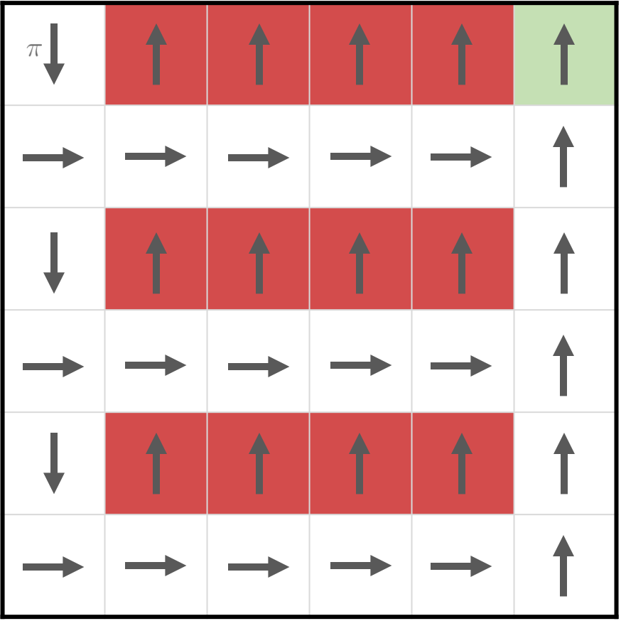
Figure 2: Modified Cliffwalk environment [Rakhsha et al., 2022].

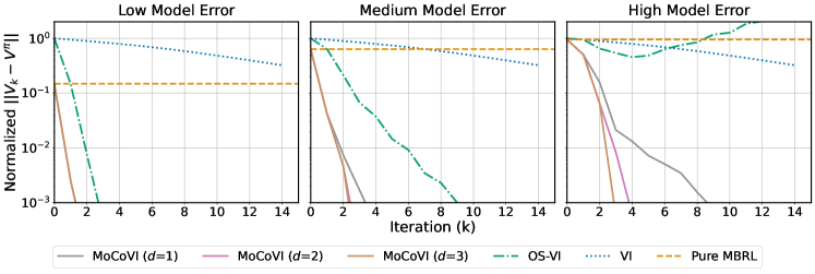
Figure 3: Policy evaluation results comparing MoCoVI with VI, pure MBRL and OS-VI. (Left) low ($\lambda=0.1$), (Middle) medium ($\lambda=0.5$), and (Right) high ($\lambda=1$) model errors. Each curve is average of 20 runs. Shaded areas show the standard error.

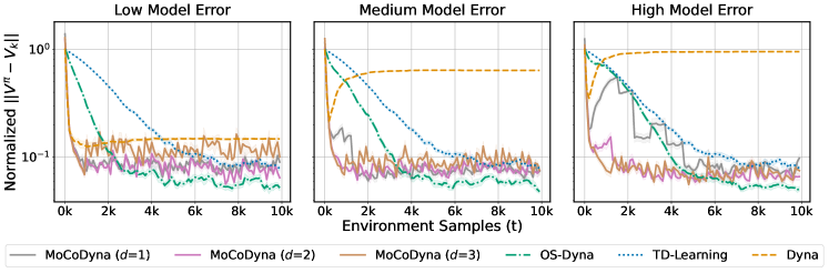
Figure 4: Policy evaluation results comparing MoCoDyna with Dyna, OS-Dyna and TD-learning. (Left) low ($\lambda=0.1$), (Middle) medium ($\lambda=0.5$), and (Right) high ($\lambda=1$) model errors. Each curve is average of 20 runs. Shaded areas show the standard error.

We perform our experiments on a $6\times 6$ gridworld environment introduced by Rakhsha et al. [2022]. The environment is shown in Figure 2. There are 4 actions in the environment: (UP, RIGHT, DOWN, LEFT). When an action is taken, the agent moves towards that direction with probability $0.9$. With probability of $0.1$ it moves towards another direction at random. If the agent attempts to exit the environment, it stays in place. The middle 4 states of the first, third, and fifth row are cliffs. If the agent falls into a cliff, it stays there permanently and receives reward of $-32$, $-16$, $-8$ every iterations for the first, third, and fifth row cliffs, respectively. The top-right corner is the goal state, which awards reward of $20$ once reached. We consider this environment with $\gamma=0.9$.

For MoCoVI, we set the initial basis functions $\phi_{i}$ for $i=1,\cdots,d$ constant zero functions. We can set $\psi_{i}=0$ for $i=1,\cdots,d$ without querying $\mathcal{P}$. This makes the comparison of algorithms fair as MoCoVI is not given extra queries before the first iteration. The convergence of MoCoVI with exact queries and $\beta=0$ is shown in Figures 1 and 3 for the control and PE problems.

Figures 1 and  4 show the performance of MoCoDyna compared to other algorithms in the PE and control problems. As discussed after Theorem 1, it is beneficial to choose basis functions such that the true value function can be approximated with $\sum_{i}w_{i}\phi_{i}$ for some small weights $w_{i}$. To achieve this in our implementation, we initialize $\phi_{1:d+c}$ with an orthonormal set of functions. Also, in line 9 of Algorithm 1, we maintain this property of basis functions by subtracting the projection of the new value function $V_{t}$ onto the span of the previous $d-1$ functions before adding it to the basis functions. We have

$$\phi_{d+c}\leftarrow V_{t}-\sum_{i=c+1}^{d+c-1}{\langle\phi_{i},V_{t}\rangle}\cdot\phi_{i},$$ (J.1)

and then we normalize $\phi_{d+c}$ to have a fixed euclidean norm. The hyperparameters of MoCoDyna for PE and control problems are given in Tables 3 and 4.

Model Error Reduction.

To show that the model correction procedure in MoCoDyna improves the accuracy of the model, we plot the error of original and corrected dynamics in the control problem in Figure 5. The model error is measured by taking the average of $\|\mathcal{P}(\cdot|x,a)-\hat{\mathcal{P}}(\cdot|x,a)\|_{1}$ or $\|\mathcal{P}(\cdot|x,a)-\bar{\mathcal{P}}(\cdot|x,a)\|_{1}$ over all $x,a$. We observe that higher order correction better reduces the error.

Computation Cost.

In Table 1 we provide the average time the calculation of $\bar{\mathcal{P}}$ has taken in MoCoDyna in the control problem. This is total time to calculate $\bar{\mathcal{P}}(\cdot|x,a)$ for all $144$ state-action pairs in the environment. In our implementation, the dual variables of the optimization problem for all state-action pairs are optimized with a single instance of the BFGS algorithm in SciPy library. Note that in general, different instances of the optimization problem (P2) for a batch of state-action pairs can be solved in parallel to reduce the computation time. Table 2 shows the full run time of the algorithms. It is important to note that in Algorithm 1, apart from reporting the current policy for the purpose of evaluation in line 6, MoCoDyna only needs to plan with $\bar{\mathcal{P}}$ every $K$ steps to have $V_{t}$ in line 9. In our implementation, planning is done every 2000 steps to evaluate the algorithm. Performing the planning only when needed in line 9 would make the algorithm computationally faster.

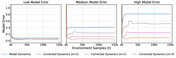
Figure 5: Comparison of the error of the original uncorrected model compared to error of corrected dynamics in the PE problem. (Left) low ($\lambda=0.1$), (Middle) medium ($\lambda=0.5$), and (Right) high ($\lambda=1$) model errors. Each curve is average of 10 runs. Shaded areas show the standard error.

Table 1: Average computation time (seconds) of $\bar{\mathcal{P}}$ during a run of algorithms in the control problem for low ($\lambda=0.1$), medium ($\lambda=0.5$), and high ($\lambda=1$) model errors.

	MoCoDyna1	MoCoDyna2	MoCoDyna3
$\lambda=0.1$	$0.24$	$0.58$	$1.51$
$\lambda=0.5$	$0.29$	$0.52$	$1.39$
$\lambda=1$	$0.2$	$0.5$	$1.44$

Table 2: Run time (seconds) for a single run of algorithms in the control problem for low ($\lambda=0.1$), medium ($\lambda=0.5$), and high ($\lambda=1$) model errors.

	TD Learning	Dyna	OS-Dyna	MoCoDyna1	MoCoDyna2	MoCoDyna3
$\lambda=0.1$	$44$	$50$	$555$	$119$	$134$	$200$
$\lambda=0.5$	$44$	$34$	$565$	$113$	$114$	$169$
$\lambda=1$	$44$	$33$	$600$	$91$	$110$	$172$

Table 3: Hyperparamters for the PE problem. Cells with multiple values provide the value of the hyperparameter for different model errors with $\lambda=0.1$, $\lambda=0.5$, and $\lambda=1$, respectively.

	TD Learning	OS-Dyna	MoCoDyna1	MoCoDyna2	MoCoDyna3
learning rate	$0.2$	$0.05,0.05,0.05$	-	-	-
$c$	-	-	$2,2,2$	$2,2,2$	$2,2,2$
$\beta$	-	-	$0.02,0.02,0.02$	$0.16,0.16,0.16$	$0.14,0.14,0.14$
$K$	-	-	$250,400,750$	$300,300,400$	$300,300,400$

Table 4: Hyperparamters for the control problem. Cells with multiple values provide the value of the hyperparameter for different model errors with $\lambda=0.1$, $\lambda=0.5$, and $\lambda=1$, respectively.

	TD Learning	OS-Dyna	MoCoDyna1	MoCoDyna2	MoCoDyna3
learning rate	$0.2$	$0.02,0.02,0.02$	-	-	-
$c$	-	-	$2,2,2$	$2,2,2$	$2,2,2$
$\beta$	-	-	$0.02,0.02,0.02$	$0.16,0.16,0.16$	$0.14,0.14,0.14$
$K$	-	-	$10k,10k,10k$	$6k,6k,6k$	$10k,10k,10k$

References

• Abachi etΒ al. [2020] Romina Abachi, Mohammad Ghavamzadeh, and Amir-massoud Farahmand. Policy-aware model learning for policy gradient methods. arXiv:2003.00030v2, 2020.
• Abachi etΒ al. [2022] Romina Abachi, ClaasΒ A. Voelcker, Animesh Garg, and Amir-massoud Farahmand. VIPer: Iterative value-aware model learning on the value improvement path. In Decision Awareness in Reinforcement Learning Workshop at ICML 2022, 2022.
• Abbas etΒ al. [2020] Zaheer Abbas, Samuel Sokota, Erin Talvitie, and Martha White. Selective dyna-style planning under limited model capacity. In HalΒ DaumΓ© III and Aarti Singh, editors, Proceedings of the 37th International Conference on Machine Learning, volume 119 of Proceedings of Machine Learning Research, pages 1–10. PMLR, 13–18 Jul 2020.
• Altun and Smola [2006] Yasemin Altun and Alex Smola. Unifying divergence minimization and statistical inference via convex duality. In Proceedings of the 19th Annual Conference on Learning Theory, COLT’06, pages 139–153. Springer-Verlag, 2006. ISBN 3-540-35294-5, 978-3-540-35294-5. doi: 10.1007/11776420_13.
• ÁvilaΒ Pires and SzepesvΓ‘ri [2016] Bernardo ÁvilaΒ Pires and Csaba SzepesvΓ‘ri. Policy error bounds for model-based reinforcement learning with factored linear models. In Conference on Learning Theory (COLT), 2016.
• Bertsekas [2009] D.Β Bertsekas. Convex Optimization Theory. Athena Scientific optimization and computation series. Athena Scientific, 2009. ISBN 9781886529311.
• Bertsekas and Tsitsiklis [1996] DimitriΒ P. Bertsekas and JohnΒ N. Tsitsiklis. Neuro-Dynamic Programming. Athena Scientific, 1996.
• Borwein and Lewis [1991] JonathanΒ M Borwein and AdrianΒ S Lewis. Duality relationships for entropy-like minimization problems. SIAM Journal on Control and Optimization, 29(2):325–338, 1991.
• Botev and Kroese [2011] ZdravkoΒ I Botev and DirkΒ P Kroese. The generalized cross entropy method, with applications to probability density estimation. Methodology and Computing in Applied Probability, 13:1–27, 2011.
• Brooks etΒ al. [2011] S.Β Brooks, A.Β Gelman, G.Β Jones, and X.L. Meng. Handbook of Markov Chain Monte Carlo. Chapman & Hall/CRC Handbooks of Modern Statistical Methods. CRC Press, 2011. ISBN 9781420079425.
• Chen and Rosenfeld [2000a] S.F. Chen and R.Β Rosenfeld. A survey of smoothing techniques for me models. IEEE Transactions on Speech and Audio Processing, 8(1):37–50, 2000a. doi: 10.1109/89.817452.
• Chen and Rosenfeld [2000b] StanleyΒ F Chen and Ronald Rosenfeld. A survey of smoothing techniques for me models. IEEE transactions on Speech and Audio Processing, 8(1):37–50, 2000b.
• Cover and Thomas [2006] ThomasΒ M. Cover and JoyΒ A. Thomas. Elements of Information Theory 2nd Edition (Wiley Series in Telecommunications and Signal Processing). Wiley-Interscience, July 2006. ISBN 0471241954.
• Dabney etΒ al. [2021] Will Dabney, AndrΓ© Barreto, Mark Rowland, Robert Dadashi, John Quan, MarcΒ G Bellemare, and David Silver. The value-improvement path: Towards better representations for reinforcement learning. In Proceedings of the AAAI Conference on Artificial Intelligence, volumeΒ 35, pages 7160–7168, 2021.
• Darroch and Ratcliff [1972] JohnΒ N Darroch and Douglas Ratcliff. Generalized iterative scaling for log-linear models. The annals of mathematical statistics, pages 1470–1480, 1972.
• Decarreau etΒ al. [1992] AndrΓ©e Decarreau, Danielle Hilhorst, Claude LemarΓ©chal, and Jorge Navaza. Dual methods in entropy maximization. application to some problems in crystallography. SIAM Journal on Optimization, 2(2):173–197, 1992.
• DellaΒ Pietra etΒ al. [1997] S.Β DellaΒ Pietra, V.Β DellaΒ Pietra, and J.Β Lafferty. Inducing features of random fields. IEEE Transactions on Pattern Analysis and Machine Intelligence, 19(4):380–393, 1997. doi: 10.1109/34.588021.
• DudΓ­k etΒ al. [2004a] Miroslav DudΓ­k, StevenΒ J. Phillips, and RobertΒ E. Schapire. Performance guarantees for regularized maximum entropy density estimation. In John Shawe-Taylor and Yoram Singer, editors, Proceedings of the 17th Annual Conference on Computational Learning Theory, volume 3120 of Lecture Notes in Computer Science, pages 472–486. Springer Berlin Heidelberg, 2004a. ISBN 978-3-540-22282-8.
• DudΓ­k etΒ al. [2004b] Miroslav DudΓ­k, StevenΒ J. Phillips, and RobertΒ E. Schapire. Performance guarantees for regularized maximum entropy density estimation. In John Shawe-Taylor and Yoram Singer, editors, Learning Theory, pages 472–486, Berlin, Heidelberg, 2004b. Springer Berlin Heidelberg. ISBN 978-3-540-27819-1.
• DudΓ­k etΒ al. [2007] Miroslav DudΓ­k, StevenΒ J Phillips, and RobertΒ E Schapire. Maximum entropy density estimation with generalized regularization and an application to species distribution modeling. 2007.
• Farahmand [2018] Amir-massoud Farahmand. Iterative value-aware model learning. In Advances in Neural Information Processing Systems (NeurIPS - 31), pages 9072–9083, 2018.
• Farahmand etΒ al. [2010] Amir-massoud Farahmand, RΓ©mi Munos, and Csaba SzepesvΓ‘ri. Error propagation for approximate policy and value iteration. In J.Β Lafferty, C.Β K.Β I. Williams, J.Β Shawe-Taylor, R.Β S. Zemel, and A.Β Culotta, editors, Advances in Neural Information Processing Systems (NeurIPS - 23), pages 568–576. 2010.
• Farahmand etΒ al. [2017] Amir-massoud Farahmand, André M.S. Barreto, and DanielΒ N. Nikovski. Value-aware loss function for model-based reinforcement learning. In Proceedings of the 20th International Conference on Artificial Intelligence and Statistics (AISTATS), pages 1486–1494, April 2017.
• Goodman [2004] Joshua Goodman. Exponential priors for maximum entropy models. In Proceedings of the Human Language Technology Conference of the North American Chapter of the Association for Computational Linguistics: HLT-NAACL 2004, pages 305–312. Association for Computational Linguistics, 2004.
• Jafferjee etΒ al. [2020] Taher Jafferjee, Ehsan Imani, Erin Talvitie, Martha White, and Micheal Bowling. Hallucinating value: A pitfall of dyna-style planning with imperfect environment models. arXiv preprint arXiv:2006.04363, 2020.
• Janner etΒ al. [2019] Michael Janner, Justin Fu, Marvin Zhang, and Sergey Levine. When to trust your model: Model-based policy optimization. In Advances in Neural Information Processing Systems, volumeΒ 32. Curran Associates, Inc., 2019.
• Jaynes [1957] E.Β T. Jaynes. Information theory and statistical mechanics. Phys. Rev., 106:620–630, May 1957. doi: 10.1103/PhysRev.106.620.
• Kakade and Langford [2002] Sham Kakade and John Langford. Approximately optimal approximate reinforcement learning. In Proceedings of the Nineteenth International Conference on Machine Learning (ICML), pages 267–274, 2002.
• Kapur and Kesavan [1992] J.Β N. Kapur and H.Β K. Kesavan. Entropy Optimization Principles and Their Applications, pages 3–20. Springer Netherlands, Dordrecht, 1992. ISBN 978-94-011-2430-0. doi: 10.1007/978-94-011-2430-0_1.
• Kazama and Tsujii [2003] Jun’ichi Kazama and Jun’ichi Tsujii. Evaluation and extension of maximum entropy models with inequality constraints. In Proceedings of the 2003 Conference on Empirical Methods in Natural Language Processing, pages 137–144, 2003.
• Kullback [1959] S.Β Kullback. Information Theory and Statistics. Wiley publication in mathematical statistics. Wiley, 1959.
• Lau [1994] Raymond Lau. Adaptive statistical language modeling. PhD thesis, Massachusetts Institute of Technology, 1994.
• Lebanon and Lafferty [2001] Guy Lebanon and John Lafferty. Boosting and maximum likelihood for exponential models. In T.Β Dietterich, S.Β Becker, and Z.Β Ghahramani, editors, Advances in Neural Information Processing Systems, volumeΒ 14. MIT Press, 2001.
• Lovatto etΒ al. [2020] Γ‚ngeloΒ G. Lovatto, ThiagoΒ P. Bueno, DenisΒ D. MauΓ‘, and LelianeΒ N. deΒ Barros. Decision-aware model learning for actor-critic methods: When theory does not meet practice. In Jessica ZosaΒ Forde, Francisco Ruiz, MelanieΒ F. Pradier, and Aaron Schein, editors, Proceedings on "I Can’t Believe It’s Not Better!" at NeurIPS Workshops, volume 137 of Proceedings of Machine Learning Research, pages 76–86. PMLR, 12 Dec 2020.
• Malouf [2002] Robert Malouf. A comparison of algorithms for maximum entropy parameter estimation. In COLING-02: The 6th Conference on Natural Language Learning 2002 (CoNLL-2002), 2002.
• Munos [2003] RΓ©mi Munos. Error bounds for approximate policy iteration. In Proceedings of the 20th International Conference on Machine Learning (ICML), pages 560–567, 2003.
• Munos [2007] RΓ©mi Munos. Performance bounds in ${L}_{p}$ norm for approximate value iteration. SIAM Journal on Control and Optimization, pages 541–561, 2007.
• Rakhsha etΒ al. [2022] Amin Rakhsha, Andrew Wang, Mohammad Ghavamzadeh, and Amir-massoud Farahmand. Operator splitting value iteration. Advances in Neural Information Processing Systems, 35:38373–38385, 2022.
• Scherrer etΒ al. [2015] Bruno Scherrer, Mohammad Ghavamzadeh, Victor Gabillon, Boris Lesner, and Matthieu Geist. Approximate modified policy iteration and its application to the game of tetris. Journal of Machine Learning Research (JMLR), 16(49):1629–1676, 2015.
• Shore and Johnson [1980] J.Β Shore and R.Β Johnson. Axiomatic derivation of the principle of maximum entropy and the principle of minimum cross-entropy. IEEE Transactions on Information Theory, 26(1):26–37, 1980. doi: 10.1109/TIT.1980.1056144.
• Sutton [1990] RichardΒ S. Sutton. Integrated architectures for learning, planning, and reacting based on approximating dynamic programming. In Proceedings of the 7th International Conference on Machine Learning (ICML), 1990.
• Sutton and Barto [2019] RichardΒ S. Sutton and AndrewΒ G. Barto. Reinforcement Learning: An Introduction. The MIT Press, second edition, 2019.
• SzepesvΓ‘ri [2010] Csaba SzepesvΓ‘ri. Algorithms for Reinforcement Learning. Morgan Claypool Publishers, 2010.
• Talvitie [2017] ErinΒ J. Talvitie. Self-correcting models for model-based reinforcement learning. In Proceedings of the Thirty-First AAAI Conference on Artificial Intelligence, pages 2597–2603, 2017.
• Voelcker etΒ al. [2022] ClaasΒ A. Voelcker, Victor Liao, Animesh Garg, and Amir-massoud Farahmand. Value gradient weighted model-based reinforcement learning. In International Conference on Learning Representations (ICLR), 2022.
• Zhang [2004] Tong Zhang. Class-size independent generalization analsysis of some discriminative multi-category classification. Advances in Neural Information Processing Systems, 17, 2004.