Evaluating VLMs for Score-Based, Multi-Probe Annotation of 3D Objects

Abstract

Unlabeled 3D objects present an opportunity to leverage pretrained vision language models (VLMs) on a range of annotation tasks—from describing object semantics to physical properties. An accurate response must take into account the full appearance of the object in 3D, various ways of phrasing the question/prompt, and changes in other factors that affect the response. We present a method to marginalize over any factors varied across VLM queries, utilizing the VLM’s scores for sampled responses. We first show that this probabilistic aggregation can outperform a language model (e.g., GPT4) for summarization, for instance avoiding hallucinations when there are contrasting details between responses. Secondly, we show that aggregated annotations are useful for prompt-chaining; they help improve downstream VLM predictions (e.g., of object material when the object’s type is specified as an auxiliary input in the prompt). Such auxiliary inputs allow ablating and measuring the contribution of visual reasoning over language-only reasoning. Using these evaluations, we show how VLMs can approach, without additional training or in-context learning, the quality of human-verified type and material annotations on the large-scale Objaverse dataset.

1 Introduction

Numerous ML applications could benefit from a zero-shot VLM pipeline to identify the type and nature of a 3D object from views of it. We assess the design choices for such a pipeline: (i) what images to use, (ii) what VLM, (iii) how to prompt the VLM, (iv) how to aggregate multi-view or multi-prompt responses to produce an aggregate, and (v) what auxiliary information can be provided to improve inference. These stages can be evaluated and optimized using sparse labeled data. But to scale VLM pipeline assessment beyond validation accuracy, we also show (vi) how to surface interesting or problematic cases by comparing VLM responses with visionless responses from the same model.

Datasets of 3D objects (e.g., Objaverse [10]) provide a controllable, rich testing ground for such a pipeline. Without loss of generality for our evaluations, we target the generation of useful text pairings for 764K objects. We look beyond captioning to infer specific properties such as type, material, physical behavior, affordances, or relations like containment between objects. These property-specific annotations (PSAs) help index the objects on a set of conceptual axes (Figure 1).

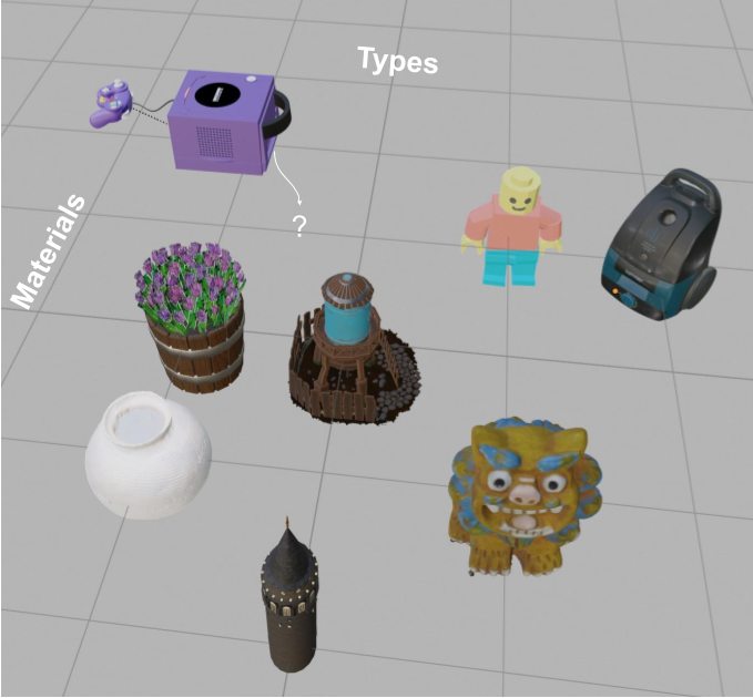
Figure 1: An inferred conceptual subgrid for 3D objects. The x-axis denotes types such as pot, tower, figurine, or appliance. The y-axis denotes materials such as brick, clay, wood, or plastic. We test VLMs on how well they infer such properties of 3D objects, using a novel likelihood-based aggregation across 2D views to avoid hallucinations. We use validation sets where possible, but also introduce an unsupervised ablation to scale VLM evaluation.

To address the challenge of inspecting a 3D object using 2D views, we generate VLM responses with accompanying log-likelihoods. This facilitates a score-based multi-probe aggregation (SBMPA) to determine the most reliable responses across different object views (or arbitrary varied factors). Our method is novel, general, and compares favorably with text-only summarization; the latter requires additional computation, some instruction tuning, yet tends to propagate upstream contradictions (i.e., hallucination). By processing individual 2D views, we can attribute an aggregate response to specific views, thus mitigating black-boxeyness.

Property-specific annotations (PSAs) not only facilitate comparison, search, and aggregation across occurrences—they also make it easier to run visual question answering in a structured, iterative manner. By specifying the value of an inferred variable in the prompt while querying for another property, we can probe VLMs in a causally driven manner. As one might expect, prompt-chaining improves the accuracy of downstream VLM inference. We compare PSAs versus descriptive object captions on the magnitude of this improvement. Despite being compared with captions containing strictly more relevant information, PSAs are on par in terms of prompt-chained VLM accuracy.

Using intermediate inferences as inputs, we can ablate the role of the assumed ancestor variable—object appearance—for subsequent inferences. This helps answer whether visual reasoning is required, or whether language-based reasoning would suffice for some properties. The ablation is especially useful when there’s no labeled data to validate inferences. We propose an unsupervised metric—to summarize the ablation—which not only correlates with validation accuracy, but also helps surface cases where visual, instance-specific reasoning diverges from language-only reasoning.

We organize the paper around the design choices we introduced for the VLM annotation pipeline. Sec 2 lays out some background and prior work. In Sec 3, we study the variation in VLM responses under changes in view or prompt, and how best to summarize responses reliably. In Sec 4, we assess prompt-chaining using previous inferred properties. Sections 3 and 4 focus on object semantics and physical material respectively, using human-verified labels to evaluate the annotations and pipeline. In Sec 5, we explore unsupervised evaluation of annotations by comparing vision-based and visionless VLM responses. Finally in Sec 6, we come back to the question of what happens if we vary the set of images we use, or vary the appearance of an object.

Our salient contributions are the following–we:

1. Run 55B-parameter variants of PaLI-X [3] to generate captions and property-specific annotations on Objaverse.

2. Introduce a likelihood-based probabilistic aggregation of VLM responses across object views and multiple queries.

3. Introduce human-validated object understanding tasks (e.g., a new test set for material inference), but also an unsupervised metric that is predictive of VLM accuracy.

4. Compare our annotations and aggregation method with concurrent work based on GPT4 (CAP3D [31]), other VLMs such as BLIP-2 [29], and baseline sources.

5. Release 350M PaLI-X responses annotating Objaverse.

2 Background

A. Multi-view differences can produce varying object descriptions

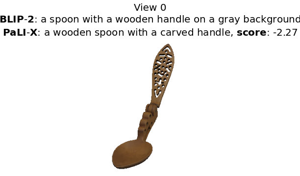
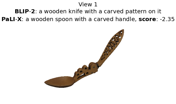
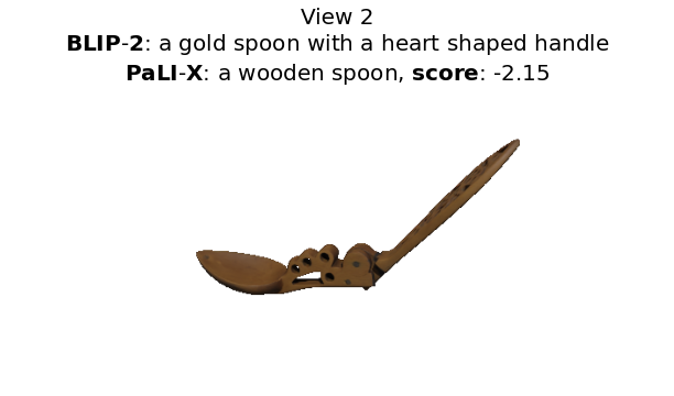
B. Aggregation in text space using an LLM and engineered prompt (CAP3D)

C. Aggregation using scores associated with each description (ours)

 

Figure 2: A. Three of eight regularly spaced views of a 3D object. Each view is accompanied by the top caption produced by two different models: BLIP-2 and PaLI-X. Captions from BLIP-2 were obtained from the contemporary CAP3D baseline [31], whereas captions from PaLI-X were generated with accompanying scores for this work. Both models show an expected variation in responses across views. B. To aggregate multi-view captions, CAP3D feeds them to GPT4 and prompts it for an object-level summary. The LLM is often unable to reconcile captions from contrasting views, and simply "adds up" the contents. C. Our aggregation produces more reliable responses, weighting them based on their combined scores across views.

Dataset. Our main target is Objaverse 1.0 [10], an internet-scale collection of 800K diverse but poorly annotated 3D models. They were uploaded by 100K artists to the Sketchfab platform. While the uploaded tags and descriptions are inconsistent and unreliable, a subset of 47K objects called Objaverse-LVIS is accompanied by human-verified categories. We rely on it to validate our semantic annotations. We also introduce a subset with material labels to test material inference. Other datasets we considered include OmniObject3D [45], ABO [6], and ScanNeRF [8]. But they lack the scale and potential of Objaverse—for instance, the number of object classes in other datasets is at most a few hundred, compared to 1156 in Objaverse-LVIS alone.

Baseline. A three-module pipeline was recently proposed to generate captions for Objaverse. Although our goals—to produce property-specific annotations and scale VLM evaluation—are meaningfully different, we rely on CAP3D [31] as the primary baseline for our work. Their pipeline is as follows: a VLM (BLIP-2 [29]) first produces 5 candidate captions for 8 object views; CLIP [38] filters all but one caption per view, and GPT4 [36] performs a flawed detail-preserving but hallucination-prone aggregation (see Sec 3). Our procedure is similar up to CAP3D’s first stage, but we don’t use any further modules for filtering or summarization.

Models. To generate our own captions or annotations, we rely on two variants of PaLI-X fine-tuned specifically for captioning or visual question answering. Both variants consist of a ViT-22B [9] vision model and 32B UL2 [43] language backbone. For material prediction, we also run BLIP-2 T5 XL [29] as a baseline. All models are run zero-shot, one input image at a time, and output an autoregressive distribution over language tokens. The likelihood of any sampled text can be computed during the VLM sampling process (e.g., beam search) without any additional cost. Since these are the only assumptions we make about VLMs, none of our methods or results are specific to PaLI or BLIP.

2.1 Prior Work

Before VLMs, one approach [19] to caption 3D shapes detected parts of an object across multiple views, then translated a sequence of view-aggregated part features into a caption. Another work [24] showed that part segmentation emerged using human text annotations to discriminate between related shapes. A recent paper [35] explored how to replicate human 3D shape understanding using multi-view learning and neurally mappable modules, but found they fell short on novel objects.

Foreshadowing the possibilities for semantic annotation of 2D images, [47] explored novel object detection using sparse bounding box annotations but extensive image-caption data. With the advent of VLMs [30, 38, 22, 28, 1, 4], more image processing and reasoning tasks came within reach: VISPROG [17] used in-context VLM learning to produce Python code to invoke off-the-shelf vision models and image processing APIs. ViperGPT [42] also showed gains in reasoning spatially or at the level of object attributes by decomposing queries into executable subroutines. Even closer to our work, [49] explored an interactive VQA approach using an LLM (ChatGPT) to ask questions about image contents, a VLM (BLIP-2) to answer them, and finally an LLM to produce a summary caption. [13] recently explored the inference of physical properties such as object material in images and collected a custom dataset to fine-tune VLMs.

Applying VLMs to 3D domains remains under-explored. [18] propose using object category labels to extract relevancy maps from 2D VLMs. These can be turned into 3D occupancies, then utilized for scene completion or object localization. [21] propose training 3D VLMs by projecting 3D feature maps to 2D and bootstrapping from a pretrained 2D VLM. The only method that contends with aggregating outputs from multiple VLM probes is ConceptGraphs [15], released when this work was submitted. Their focus is on building open-vocabulary scene graphs to help with navigation tasks in larger environments, which is different from our objective of generating object-centric, property-specific annotations.

3 Appearance $\rightarrow$ Type(s)

Our first task is to infer the type of each Objaverse object in a zero-shot, open-vocabulary setting. The task is compelling because only $\sim 5\%$ of Objaverse is accompanied by category labels. Being able to predict them without training would help shed light on the rest of the dataset. We also expect asking for the type of an object to be a language-amenable query, and hence a basic test for VLMs.

Despite how simple a task this initially appears, the challenge of captioning a 3D object is evident from Fig 2-A. Recent work (CAP3D [31]) to produce captions for Objaverse relies on GPT4 [36] to summarize annotations across multiple views of an object. This can produce deeply flawed summaries. The LLM propagates hallucinations or confusions when there’s contrasting captions among views. Despite being instructed that it is given captions of the same object, the LLM tries to preserve details across views rather than reconcile them (see Fig 2-B).

To address this, we propose an alternative method of aggregating multi-view or multi-query annotations (see Fig 2-C). We describe the method in Sec 3.1. We compare semantic descriptions from baseline sources with annotations produced by our method in Sec 3.2. Finally, we unpack the performance of our aggregation relative to individual views or queries in Sec 3.3.

\begin{overpic}[width=496.85625pt,percent]{figures/caption_similarity_lvis.png} \put(9.0,20.0){\includegraphics[scale={0.34}]{figures/caption_similarity_lvis_example_object.png}} \end{overpic}

	Objaverse tags	PaLI VQA
Top-1 acc.	$0.06\pm 0.24$	$0.26\pm 0.44$
Top-5 acc.	$0.13\pm 0.34$	$0.52\pm 0.50$
Top-$\infty$ acc.	$0.15\pm 0.36$	$0.67\pm 0.47$
Soft acc.	$0.04\pm 0.17$	$0.19\pm 0.26$

Figure 3: Comparison of captions and type annotations generated from different sources/models. All results are averaged over Objaverse-LVIS. Left: the bars show text-embedding similarity scores ($\uparrow$) for the aggregate/top per-object descriptions from each source. We show an example caption/type annotation beneath each bar; these correspond to a fixed object shown in the upper left corner from two different views. Right: string-match metrics that assess full predicted distributions from two sources. We report top-k accuracies (whether the correct type is in the top-k predictions, $\uparrow$) as well as the soft accuracy (probability of the correct type in the output distribution, $\uparrow$).

3.1 Score-Based Multi-Probe Aggregation

We introduce a method for aggregating VLM outputs across multiple queries that relies on the log-likelihoods or scores of the sampled outputs. When VLM queries are correlated (e.g. views of the same object or paraphrased questions), we can expect recurring responses across queries. Say we run I queries to get J (response, score) pairs per query, for a total of IJ pairs $\{(r_{i,j},s_{i,j})\}$. Let $f$ be a map to postprocess strings and reduce them to a canonical form. The following aggregation helps identify responses $r$ which occur frequently while accounting for the model’s confidence in each occurrence. $\forall r\in\{r_{i,j}\}$:

$$s_{i}(r)\vcentcolon=\sup\{s_{i,j}\mid f(r_{i,j})=r\textrm{ and }j=1,2,...,J\}$$ (1)

$$s_{agg}(r)\vcentcolon=\log\sum_{i}\exp(s_{i}(r))$$ (2)

$$p(r|\{r_{i,j},s_{i,j}\})\vcentcolon=\exp(s_{agg}(r))/\sum_{r^{\prime}}\exp(s_{agg}(r^{\prime}))$$ (3)

Equation 1 deduplicates and re-scores responses for a given VLM query $i$. The string processor $f$ determines when $r_{i,j}$ is treated equivalent to $r$, and can be customized per VLM. This is useful when responses are identical up to punctuation, case, or uninformative tokens. Since these are undesirable duplicates, we want to avoid accumulating their scores, so we take the supremum instead. Note that $s_{i}(r)$ can be $-\infty$ if no $r$ equivalent occurs in the J responses for query $i$.

Equation 2 then aggregates scores across occurrences of $r$ in distinct queries. These are desirable duplicates (over distinct images or prompts) which merit reinforcing. Finally, Equation 3 computes an aggregate probability distribution over responses by taking a softmax over the aggregate scores.

Compared to model-based summarization (e.g., using an LLM), this aggregation requires a trivial numerical computation. There’s no scoring cost in addition to generating the outputs. Whereas an LLM needs a prompt specific to the aggregation task, our method can be used on arbitrary VLM responses that need aggregating. While an LLM produces a point estimate, our method outputs a distribution over all possible responses. Although in our work we inherit any potential flaws in the VLM’s scoring, it would be straightforward to decouple the two VLM outputs—we could score $\{r_{i,j}\}$ using a different model and replace $\{s_{i,j}\}$ before Eq 1.

3.2 Type Prediction Results

We collect four sets of semantic descriptions for Objaverse:

1. Objaverse tags (baseline): these were uploaded by the creator of each 3D asset (Sec 2). They are inherently noisy and inconsistent between objects. We comma-separate the tags to produce an aggregate string for each object. But where we compute distributional metrics, we treat the tags separately, as ordered but uniformly likely.

2. CAP3D captions (baseline): these were generated and released by [31]. A post-processed version removes the frequent prefix, “3D model of” (we compare both versions).

3. PaLI captions (ours): using a captioning variant of PaLI and simple prompt (“A picture of ”), we generated descriptive captions similar to CAP3D’s first stage. We then applied our aggregation to summarize $J=5$ responses across $I=8$ views per object. We compare results with and without a post-processing map $f$ (Eq 1) to ignore suffixes of the form “on/against a white background.”

4. PaLI VQA annotations (ours): we used 4 VQA prompts to probe for the type of each object: (i) What is this? (ii) What type of object is this? (iii) What is in the image? (iv) Describe the object in the image. This produced 4 sets of top-5 responses per view ($I=4*8=32,\ J=5$). The responses are typically WordNet [33] entities that group synonyms or related terms in a comma-separated list. We deduplicate responses by taking the first such term per response. This post-processing map is also ablated.

We compare outputs from these sources to human-verified object categories from the Objaverse-LVIS subset. For our sources, we take the likeliest output from each aggregate distribution. We proceed to embed all text using an independent language encoder, the Universal Sentence Encoder (v4) [2] from TensorFlow-Hub. Then, we compute cosine similarities between the embedded outputs and verified categories.

Fig 3-L shows that all VLM pipelines outperform tags from the original dataset. PaLI captions, with our score-based aggregation, are slightly better than (the three-module) CAP3D captions. PaLI VQA annotations perform significantly better than either of these: our aggregate output distributions contain the exact expected type on two-thirds of Objaverse-LVIS (see Fig 3-R). The average soft accuracy (19%) is significant considering there are up to $IJ=160$ unique responses in each aggregate output distribution.

3.3 Why Aggregate

To show why our aggregation works, we look at the individual views and queries that comprised our PaLI VQA annotations. Fig 4 shows the effect of aggregating across various slices of the views and questions presented to the VLM. We also compare our default log-sum-exp (LSE) aggregation with the simpler choice of taking the maximum score across all views/questions in Eq 2.

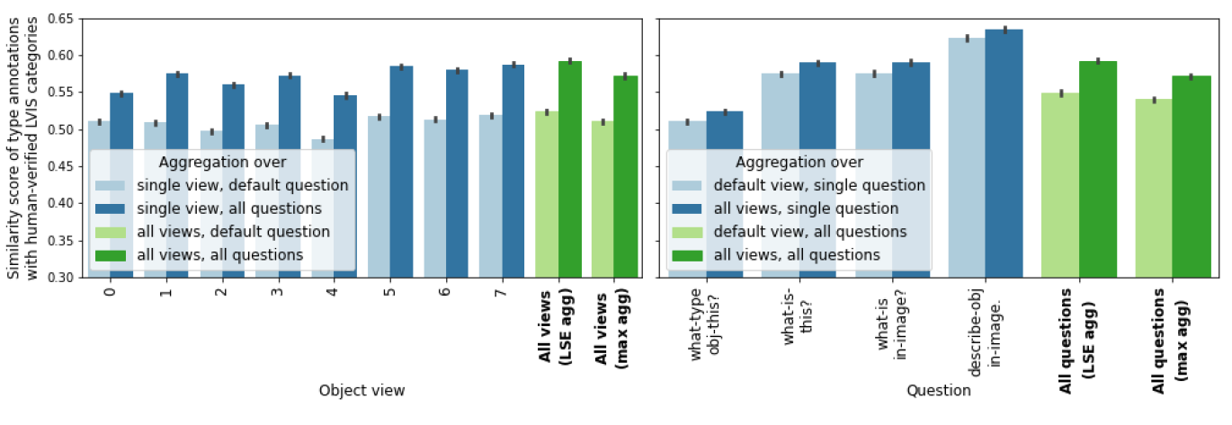
Figure 4: Score-based aggregation across views and across questions. Each bar aggregates a different subset of VLM responses. The mode of each aggregate output distribution is scored using cosine similarity on Objaverse-LVIS as before. Left: we score 8 individual views and the aggregate(s) of all views, while highlighting the gap between asking a default question or multiple question variants. Right: we score 4 individual questions and the aggregate(s) of all questions, while highlighting the gap between using a fixed object view or all views.

There’s a small but significant gap between the LSE and maximum-score aggregations. The latter performs worse than several views individually, because overconfident responses might dominate the aggregate. The LSE aggregation performs better than any individual view.

Comparing different questions, there is in fact a particular question which serves as the best VLM prompt for our current evaluation metric (cosine similarity with respect to LVIS categories). Including less optimal questions in our aggregation does not improve the score. Nevertheless it smoothens the aggregate response distribution and widens the support. We show this qualitatively in Fig 5. Aggregating across questions helps avoid mode collapse in bimodal cases (such as the bee on the wall), or smoothen over question-specific biases (e.g., questions that include the word “object” make the VLM likelier to say “toy,” while remaining questions are likelier to elicit “statue” or “lion.”)

With robustness in mind, we include all questions and object views when aggregating PaLI VQA annotations. Ultimately the goal is to produce an intermediate representation suitable for multiple tasks. To that end, we will test our aggregate type annotations on downstream inference of properties in the next section.

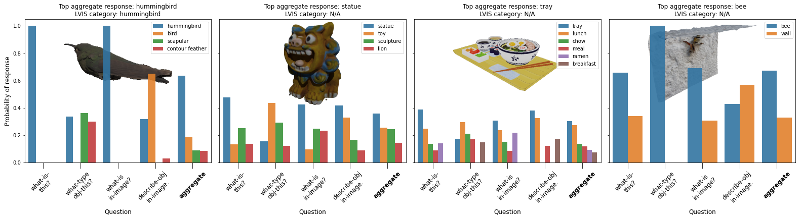
Figure 5: PaLI VQA responses per question and after aggregation for fixed views of a selection of objects. To reduce visual clutter, we filtered responses with scores below a fixed threshold (-1.2). Each subplot legend lists the possible responses sorted by aggregate probabilities. For comparison, we show the object’s LVIS category where available.

4 Appearance $\rightarrow$ Type(s) $\rightarrow$ Material

Our second task is to infer what each Objaverse object is made of. The task is significant because an object’s physical composition has immediate implications for how it behaves physically. Whether it will sink, bounce, stretch, or crack is largely determined by its material. There is limited prior work to study whether VLMs can infer material properties [13], possibly due to a lack of validation data.

Structured probes. We expect material to be less amenable to description in language than type; this raises the question whether we should prompt a VLM to reason deeper about material. One way to do this is to equip the VLM with prior inferences about the object. Concretely, we ask what material something is made of while including the object’s type in our question. Thus, the VLM can make its prediction on the basis of two factors: object type and appearance.

We ablate the influence of each factor on the VLM as follows: we pose questions including or excluding the object type (e.g., “what material is the spoon made of” vs “what material is this made of”). We also run a third probe including object type in the question but without any image input (e.g., “what material is a spoon made of”). This makes the model operate as an LLM, with the same model weights, and helps measure the accuracy of language-only reasoning.

When specifying the object’s type as part of a question, we can choose to use detailed captions like CAP3D’s, or succinct type annotations as produced by our VQA pipeline (see Sec 3.2). We study which of these performs better (but refer to them as “type annotations” collectively). To ensure our results are not specific to a model class or size, we run all evaluations on two VLMs: PaLI-X VQA as before, and the smaller BLIP-2 T5 XL (used in CAP3D).

Data/metrics. To measure material prediction accuracy, we curate a test set of 860 objects spanning 58 material classes. All labels are derived from Objaverse tags (see the Appendix for details). Unlike in Sec 3.2, we cannot rely on similarity in text embedding space because materials can appear close even when they are different (e.g. "wood" and "metal" have a cosine similarity score of 0.408). So we look for an exact string match in the VLM responses.

Results. Table 1 reveals impressive material prediction abilities in both VLMs (up to 87% top-3 accuracy from PaLI-X or 51% soft accuracy from BLIP-2). It confirms that using type annotations and object appearance simultaneously generally outperforms using one or the other. This reasoning advantage is reminiscent of chain-of-thought prompting [23] or iterative inference [14, 32]. Having access to previous computations can help the VLM avoid redundant processing.

The "From Type" sub-columns confirm that CAP3D captions contain more material information than PaLI-VQA types (in fact, 43% of CAP3D captions already contain the expected material label, versus 12% for PaLI types mainly due to objects like “iceberg” or “woodcarving”). Yet PaLI types are on par with CAP3D captions in terms of prompt-chained accuracy when we do use the object’s appearance (see "From Type and Appearance" sub-columns). This could be explained by hallucinations or specious details in CAP3D captions which hinder VLM reasoning. It goes to suggest that property-specific annotations serve as more robust intermediate representations for downstream tasks.

Table 1: Material inference with two VLMs: PaLI-X and BLIP-2.. The models are provided either an object type annotation or image as inputs or both. We report the top-3 accuracy as well as the soft accuracy averaged over our material test set of 860 objects. Whenever we use appearance as an input (i.e., VLM mode), we aggregate responses across object views. Thus the predicted distributions contain up to J=5 alternatives in LLM mode or up to IJ=40 in VLM mode.

		From Type (LLM mode)		From Appearance (VLM mode)	From Type and Appearance (VLM mode)
		CAP3D captions	PaLI-VQA types	No caption/type information	CAP3D captions	PaLI-VQA types
PaLI-X 55B VQA	Top-3 acc.	$0.73\pm 0.44$	$0.58\pm 0.49$	$0.83\pm 0.37$	$\mathbf{0.87\pm 0.34}$	$0.86\pm 0.35$
	Soft acc.	$0.36\pm 0.29$	$0.25\pm 0.28$	$0.41\pm 0.28$	$\mathbf{0.44\pm 0.27}$	$\mathbf{0.44\pm 0.29}$
BLIP-2 T5 XL	Top-3 acc.	$0.24\pm 0.43$	$0.22\pm 0.41$	$0.68\pm 0.47$	$0.59\pm 0.49$	$\mathbf{0.69\pm 0.46}$
	Soft acc.	$0.19\pm 0.35$	$0.16\pm 0.33$	$0.50\pm 0.41$	$0.42\pm 0.42$	$\mathbf{0.51\pm 0.42}$

5 Appearance $\rightarrow$ Type, Material $\rightarrow$ Others

VLMs can be probed to answer arbitrary questions. But we often lack data to validate or improve their responses. What we might have are some intermediate inferences which are already validated. We introduce a method to use these to highlight interesting or problematic VLM responses in the unsupervised case.

As in Sec 4, we can run VLMs with and without any visual input by supplying a value for the type property in both cases. The question changes slightly to be type-specific in LLM mode rather than instance-specific in VLM mode. We can then compare output distributions from running in VLM and LLM modes. To measure the divergence, we can rely on a probability metric such as the Hellinger distance.

While such a distance can be computed for any VLM in any unsupervised case, the question that arises is whether the distance correlates with the VLM’s predictive performance. Since the contribution of a VLM’s visual branch is generally residual (i.e., via cross-attention from the language branch), we posit that when answers differ between the visionless and vision-based conditions, the vision-based VLM output is likely more accurate.

We first use our material prediction accuracies (from Sec 4) to probe and motivate the use of our unsupervised metric in Figure 6(a). We find sufficient correlation between the two despite some noise in the material labels—the vision-based material predictions are often justifiably multi-modal (see Figure 6(b)) whereas our labels are one-hot.

Having shown its usefulness on material, we assess the divergence of VLM responses from their language-only counterparts on other properties (Table 2). We infer (i) binary properties such as fragility or lift-ability, (ii) open-vocabulary properties such as color and affordance, and (iii) relations between objects such as what a given object might contain.

We find that the standard deviation of Hellinger distances for any given question is indicative of the size of the output space (e.g., binary-response questions have the lowest spread). We also find that the mean of Hellinger distances grows as expected with the difficulty of answering questions in visionless mode (e.g., color benefits the most from VLM mode). Lastly, we find that providing more information in the question (both material and type rather than type alone) consistently reduces the gap (i.e., Hellinger mean) between VLM and LLM mode responses.

Our analysis is useful not only to compare questions in aggregate, but also to highlight individual cases which merit attention (see Figure 6(c)). For that reason, the analysis could be instrumental in scaling VLM annotation to unsupervised cases well beyond the scope of human-powered validation.

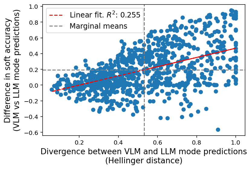
(a) VLM prediction accuracy when the VLM diverges from underlying language-only predictions. We show all datapoints from the material validation set, with a linear fit to highlight the correlation.

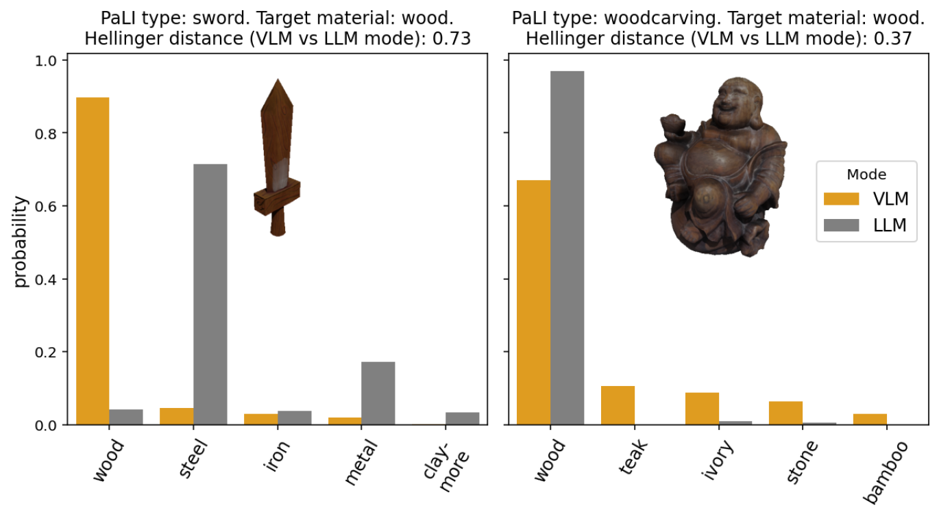
(b) Single-prompt material predictions. We show outputs over 2% prob.

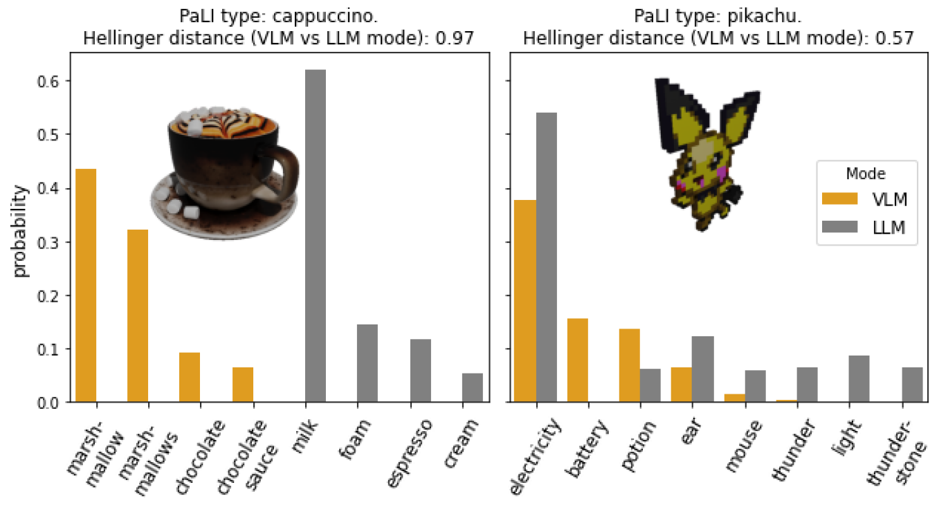
(c) Three-prompt containment predictions. We show outputs over 5% prob.

Figure 6: VLM vs LLM mode Hellinger distances. VLM mode results are view-aggregated. In (c), they are also prompt-aggregated.

Table 2: Object properties assessed without validation, via visual ablation of PaLI-X responses. Placeholders such as T or M are filled in with a prior type or material inference. The indefinite article “a” is replaced with “an” if the next word requires it.

Question type	LLM mode / VLM mode question	Hellinger distance (b/w LLM & VLM mode outputs)
Fragility	Is a/this T fragile?	$0.110\pm 0.058$
	Is a/this M T fragile?	$0.103\pm 0.054$
Lift-ability	Can a human lift a/this T?	$0.133\pm 0.063$
	Can a human lift a/this M T?	$0.124\pm 0.055$
Afford-ance	How is a/the T typically used?	$0.575\pm 0.223$
Contain-ment	What might a/the T contain?	$0.690\pm 0.260$
	What is something that typically goes into a/the T?	$0.570\pm 0.235$
	What items or substance might a/the T contain?	$0.731\pm 0.236$
Color	What color is a/this T?	$0.894\pm 0.163$
	What color is a/this M T?	$0.875\pm 0.173$

6 Appearance(s) $\rightarrow$ Type

So far we have assumed a given set of images per object. That is a limiting assumption for user-driven, real-time object annotation. In this section we explore VLM sensitivity to image and camera settings (such as lighting, poses) as well as changes to the object’s appearance (such as untextured rendering). See Table 3.

First, we are interested in how much VLMs and their underlying ViTs rely on texture to recognize objects versus shape [20, 34, 9]. We render all objects without colors and lighting (using Blender’s Workbench engine) to compare with the default appearances. The untextured images do hurt PaLI’s type prediction performance but the effect is small enough to suggest that PaLI is largely shape-driven.

Another reason for the reduced impact of untextured rendering is that a number of Objaverse models are already untextured. We suspect that lighting conditions will make a difference in recognizing these objects, because they are prone to losing detail with brightness. We render all objects with three different scene lighting choices: (i) eight area lights and one ceiling light surrounding the object, (ii) a stationary light placed higher than the camera’s initial position to enhance shadows, (iii) a moving backlight that stays at the same relative position with respect to the camera as we move it. (i) and (iii) ensure symmetry of lighting across the eight views we render, whereas (ii) makes an object look darker from “behind.” We find these intuitions do translate to slight performance gains in recognizing objects. And for the same reasons, placing objects on dark backgrounds (rather than a constant white) also helps.

Lastly, we revisit our choice of camera poses for image collection. Our aim was to encourage overlap in VLM responses to ensure the most reliable responses can “win” during aggregation. So we took images from regular yaw intervals on a circle around the object. But there are other possible schemes, e.g., one might maximize the information content of each view by prioritizing atypical object views. CAP3D took this alternative approach, varying camera height simultaneously with yaw to include top and bottom views of the object. Though we didn’t have access to the original images from CAP3D, we reverse-engineered their camera poses, and found that our choice worked better with our method. We also varied the free parameter in our choice, i.e., the polar angle at which the camera is placed facing the object. This didn’t make much difference.

On the whole, we found PaLI to be quite robust to the visual and image settings which affect object appearance.

Table 3: VLM sensitivity to image conditions and object appearance. We collect and score PaLI VQA type annotations using cosine similarity on Objaverse-LVIS. All results are view-aggregated.

Hyperparameters	PaLI VQA type similarity score
Object appearance Textured (Cycles) Untextured (Workbench)	$\bf{0.593\pm 0.290}$ $0.549\pm 0.289$
Scene lighting Surround area lights Stationary point light Camera backlight	$0.580\pm 0.291$ $0.586\pm 0.291$ $\bf{0.593\pm 0.290}$
Image background Black (0, 0, 0) Dark grey (100, 100, 100) White (255, 255, 255)	$0.603\pm 0.296$ $\bf{0.612\pm 0.294}$ $0.593\pm 0.290$
Camera poses CAP3D (incl. top & bottom views) Ours (constant polar angle)	$0.588\pm 0.290$ $\bf{0.593\pm 0.290}$
Camera polar angle $\theta$ 64 degrees 68 degrees 72 degrees	$0.591\pm 0.291$ $0.593\pm 0.290$ $\bf{0.593\pm 0.290}$

7 Limitations and Future Work

At present we hand-picked the number of views and engineered the number and wording of questions used to collect VLM annotations. In the future this could be automated using the aggregate probability distribution to determine when additional VLM responses may be required (e.g., when the entropy is large). Variations of a question could also be generated automatically using an LLM.

Perhaps the community will soon have access to VLMs which could process multi-view images simultaneously and produce a global response. While this would be an interesting direction, there is still value in less black-box approaches like ours. The SBMPA method is transparent and helps balance contradicting signals.

Before this work can be applied to object identification using arbitrary images (e.g., from a mobile camera), it would be useful to develop a measure of the marginal value of specific new views or object complexity as a whole. Nonetheless, we hope our pipeline optimization approach will transfer to scene understanding beyond digital 3D objects.

8 Conclusions

We generated property-specific annotations for 3D objects using VLMs which take in a single image and text-based prompt. We probed for properties that are increasingly inaccessible to language-based reasoning, from semantic type to material composition. We evaluated what VLMs are sensitive to, including changes in object view, question wording, prior inferences specified in the prompt, and access to the object’s appearance. We highlighted the value of marginalizing over some of these factors to produce an aggregate response, akin to how humans might arrive at an inference by examining an object from multiple angles.

We hope our outputs serve a variety of downstream 3D applications (from retrieval to 3D generation, from physical simulation to neuro-symbolic processing); and that our evaluations and insights may help shape VLM annotation pipelines in other contexts.

Supplementary Material

Appendix A Outline

We provide model and dataset details in Sections B and C respectively. We develop a measure of CAP3D’s hallucination problem in Sec D.1. Finally, we assess all our annotations qualitatively in Sec D.3.

Appendix B Model Details

We used the following VLMs off the shelf without tweaking:

B.1 PaLI-X

The model [3] is based on the flaxformer transformer [44] library and t5x training/evaluation infrastructure [40], both written and released in jax [12]. The captioning- and VQA-tuned variants have a common architecture. Checkpoints and configs for the 20B UL2 [43] language backbone are separately available here. The language backbone relies on a SentencePiece tokenizer [25] with vocab size 250K available here. The visual backbone for PaLI-X (a ViT-22B [9]) includes an additional OCR-based classification pretraining task on WebLI images [4] beyond the original JFT-3B [41, 48] image classification task.

During VLM training, the captioning and VQA variants diverge in their image resolutions ($672^{2}$ versus $756^{2}$) and training task mixtures. While the VQA variant was partly trained using the Object-Aware method [37] to detect or list object classes on the OpenImages V4 dataset [26], we are not aware of any other reason PaLI-X would be predisposed to predict object labels accurately, especially on the long-tailed distribution of Objaverse.

PaLI scoring is length normalized as originally described in Eq 14 of [46] or coded in t5x here. This is to help ensure that longer outputs are not disadvantaged. We kept the length norm parameter fixed at $\alpha=0.6$ and used default beam searching sampling with 5 parallel decodings.

B.2 BLIP-2

As CAP3D did, we use BLIP-2 from LAVIS [27], which is based on the widely used PyTorch transformers library. The model is appealing because it was shown to perform better than 54x larger models on VQA and image captioning. Its FlanT5 encoder-decoder backbone [5] was pretrained using the span corruption objective (introduced in T5 [39]), then instruction-finetuned for various language-based question answering. The image encoder is a ViT-g/14 model, as trained by EVA-CLIP [11].

Unlike PaLI-X components, BLIP-2’s ViT was directly evaluated for object detection and instance segmentation on LVISv1.0 [16]. The authors highlighted emergent capabilities on object-level instance segmentation; their ViT classified 1200 LVIS categories as accurately as the 80 COCO categories on which it was trained [11]. We expect BLIP-2 to exhibit some transfer to Objaverse-LVIS. So it is surprising that PaLI-X outperforms BLIP-2 nonetheless. Besides model size, a reason for the performance gap could be that BLIP-2 operates with images of size $224^{2}$.

We tweaked BLIP-2’s code slightly to (i) generate outputs with accompanying scores, using existing functionality in the transformers library; and (ii) optionally run in LLM mode, by removing visual tokens from inputs to the transformer. We attach the diff for these changes, totaling 20 lines, in blip2-code_diff.txt.

Appendix C Dataset Details

C.1 Objaverse Rendering

We downloaded 798,759 Objaverse GLB files and rendered them using Blender $3.4$ [7]. We dropped animations while rendering, because they pose an issue for computing bounding boxes to center objects. This produced 763,844 objects rendered from 8 different views, including 44,199 with LVIS categories.

Rendering process. We placed each object at the origin and scaled its maximum dimension to 1. We then rotated the camera at a fixed height and distance to the origin, rendering images at azimuthal intervals of 45 degrees. To determine the camera height, we swept over a few values of the polar angle $\theta$ w.r.t. the z-axis. We presented this sweep and other rendering hyperparameters (such as lighting conditions) in Table 3 in the main text.

Reproducing CAP3D views. CAP3D uses a distinct image rendering pipeline. While we render images at a fixed camera height, CAP3D images include top-down and bottom views of the object. Although we did not have access to their original images, we compared rendered images and approximated their camera poses from Fig 23 in the CAP3D paper. By default, only views 1, 3, 5, and 7 (zero-indexed) from our pipeline are comparable to 4, 3, 5, and 2 from the CAP3D pipeline.

C.2 Material Test Set

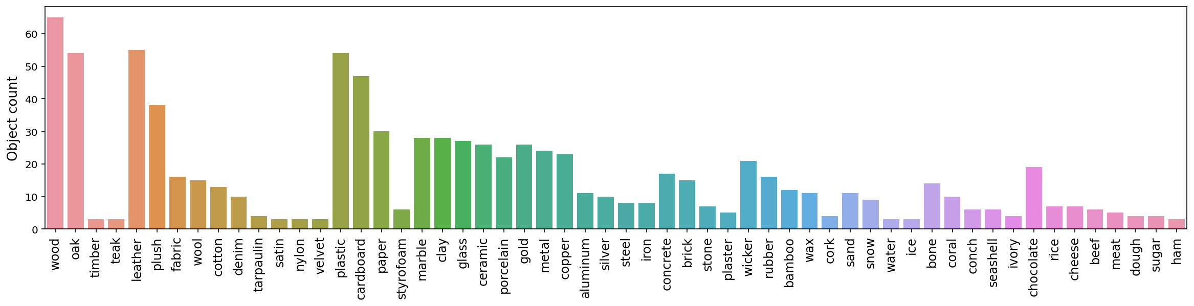
Figure 7: Our long-tailed material test set comprising 58 material classes (on the x-axis) and 860 objects.

We took inspiration from the long-tailed distribution of LVIS categories [16] to enumerate material classes for our test set. We include a range of materials with different properties: non-rigid materials (e.g., ‘tarpaulin’, ‘snow’), organic materials (e.g., ‘bamboo’, ‘seashell’, ‘bone’), manufactured materials (e.g., ‘glass’, ‘plastic’, ‘steel’), food ingredients (e.g., ‘chocolate’, ‘rice’), fabrics (e.g., ‘wool’, ‘denim’), and natural elements (e.g., ‘sand’, ‘ice’). We included labels at different levels of specificity (e.g., ‘metal’ and ‘aluminum’) because we expect aggregate predictions from a VLM to place probability mass on both levels (varying based on the VLM’s confidence). We also include labels which are easily conflated (e.g., ‘coral’, ‘seashell’, and ‘conch’).

Recipe. Rather than label objects on our own, we searched through object tags from Objaverse for a superset of 122 material labels. The initial matches were noisy—the tags often contain spurious materials (because artists can add arbitrary tags to optimize search engine visibility for their objects). So we used a custom web app to accept or reject object-label pairs from the initial matches. This helped preserve the natural, long-tailed distribution of material tags in the dataset (that also reflects the real world). We dropped query terms which returned too few/poor quality matches. In some cases, we had to resolve multiple tag matches per object. Although this was an opportunity to test multi-label prediction (which our aggregate VLM predictions do facilitate), for now we chose to focus on the primary/dominant material of each object. Finally, we merged some near-duplicate labels that we included initially to increase matches.

The final test set contains 860 objects spanning 58 classes, with at least 3 objects per class, as shown in Figure 7. See the attached file material_test_set_objects.pdf for images of all objects in the test set. See also Appendix D.2 for examples of PaLI-X and BLIP-2 predictions.

Appendix D Extended Results

D.1 Tracking Hallucination

Table 4: CAP3D captions versus ours, compared on the frequency of satisfying undesirable criteria ($\downarrow$). We use the aggregate, post-processed captions in each case—CAP3D drops prefixes like "3D model of," whereas we remove suffixes like "on a white background" from PaLI captions using Eq 1. We count captions that meet the listed criteria, then normalize by the full size of Objaverse (798,759). We use case-insensitive keyword searches unless marked with an asterisk *.

Captions that…	Cap3D	PaLI captions
Are missing/empty	17.17%	4.37%
Contain undesirable keywords: "object" "model" / "3D" "royalty-free" / "royalty free" "download" / "sale" "OBJ" / "FBX" / "C4D" / "Blender" / "Maya" (but not "Mayan")	2.95% 2.90% 0.42% 0.19% 0.14%	9.45% 0.89% 0.00% 0.00% 0.00%
Start with a word other than "a" / "an" / "the" / "two"	32.59%	5.79%
End with "background" or "background."	0.45%	0.15%

First, we develop a metric to identify cases where CAP3D hallucinates. Given a high-precision indicator, we can systematically compare those cases with our captions, and avoid cherry-picking examples. We observe that CAP3D’s GPT4 outputs are often longer than the per view captions fed to it, because GPT4 naively adds up details/contents from different views. So if we take the word count of a GPT4 output summary, and divide it by the maximum word count across all single-view captions for the same object, we can measure the blow-up in caption size due to the aggregation step.

$$\text{blow-up ratio}(r)=\dfrac{\text{word\-count}(r)}{\max_{i,j}\text{word\-count}(r_{i,j})}$$ (4)

Since we do have all aggregate and single-view captions released by CAP3D, we can compute the caption blow-up ratio for every object. We find ratios as high as 5.6, implying that GPT4 accumulated all the words of at least 5 single-view captions for that particular object. On the other hand, if we were to compute caption blow-up ratios for our pipeline, we would always get a ratio of 1.0, because our final caption is always one of the single-view captions.

We visualize objects with the highest CAP3D blow-up ratios in Figure 9, comparing CAP3D aggregate captions with ours. Across the board, our captions are more concise and accurate. We also find groups of similar objects emerging when we rank objects using the CAP3D blow-up ratios (even in the top 18 objects), suggesting systematic CAP3D errors. For instance, looking at our captions in Fig 9, we find two “silhouette” figures, two “cartoon birds”, and two “child’s drawings”.

While a high blow-up ratio seems to be a reliable indicator of hallucination, it has low recall, because even shorter CAP3D summaries can contain contradictions (e.g., “a banana and a chicken” in Figure 3). To focus on such cases which are not picked up by the caption blow-up ratio, we pick a few examples and visualize them in Figure 11. Here we also show single-view captions from both pipelines to illustrate where the aggregates come from. We show only those views which are comparable between the two pipelines. With these cases, we also include the two specific examples presented as failure cases in the CAP3D paper.

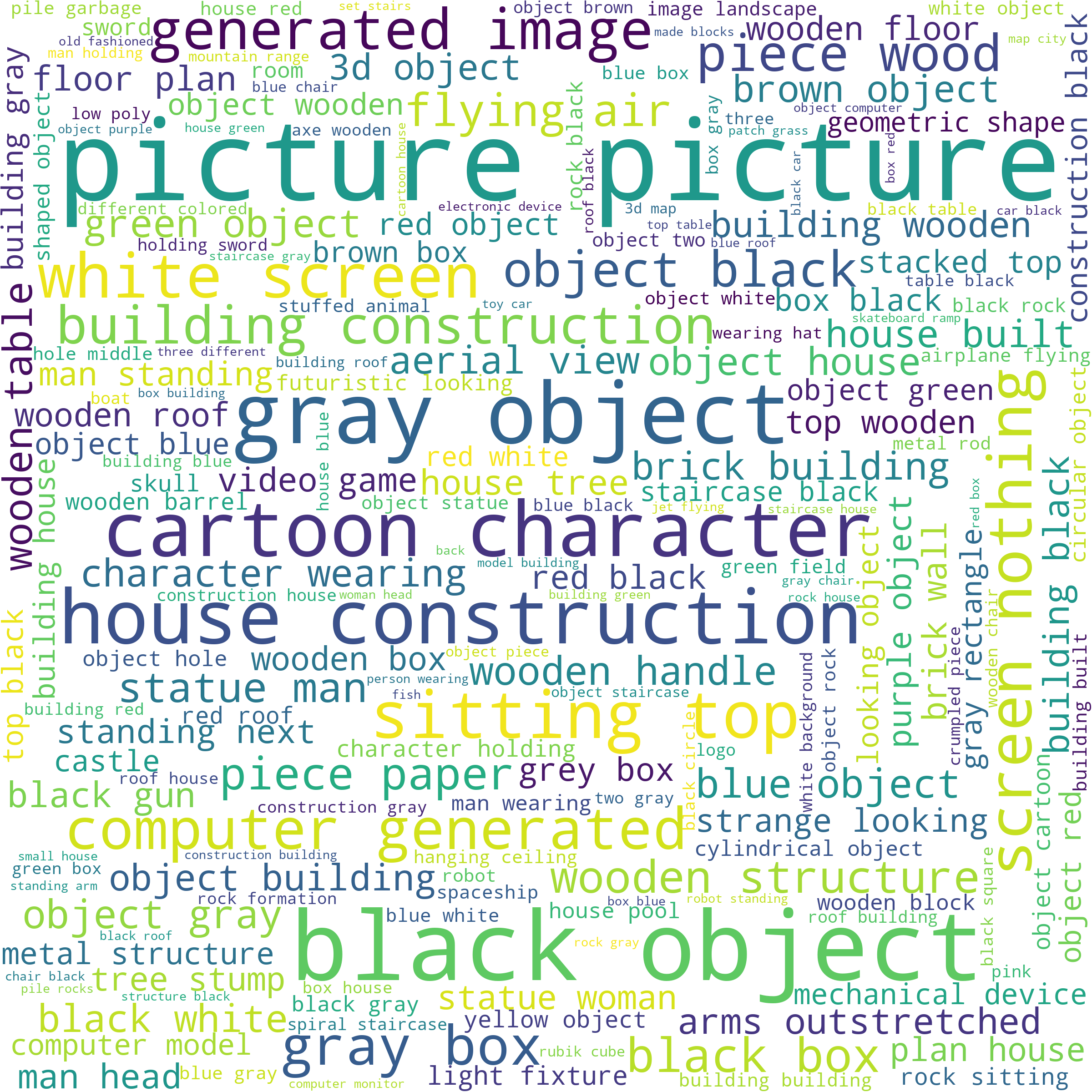
(a) PaLI aggregate top captions.

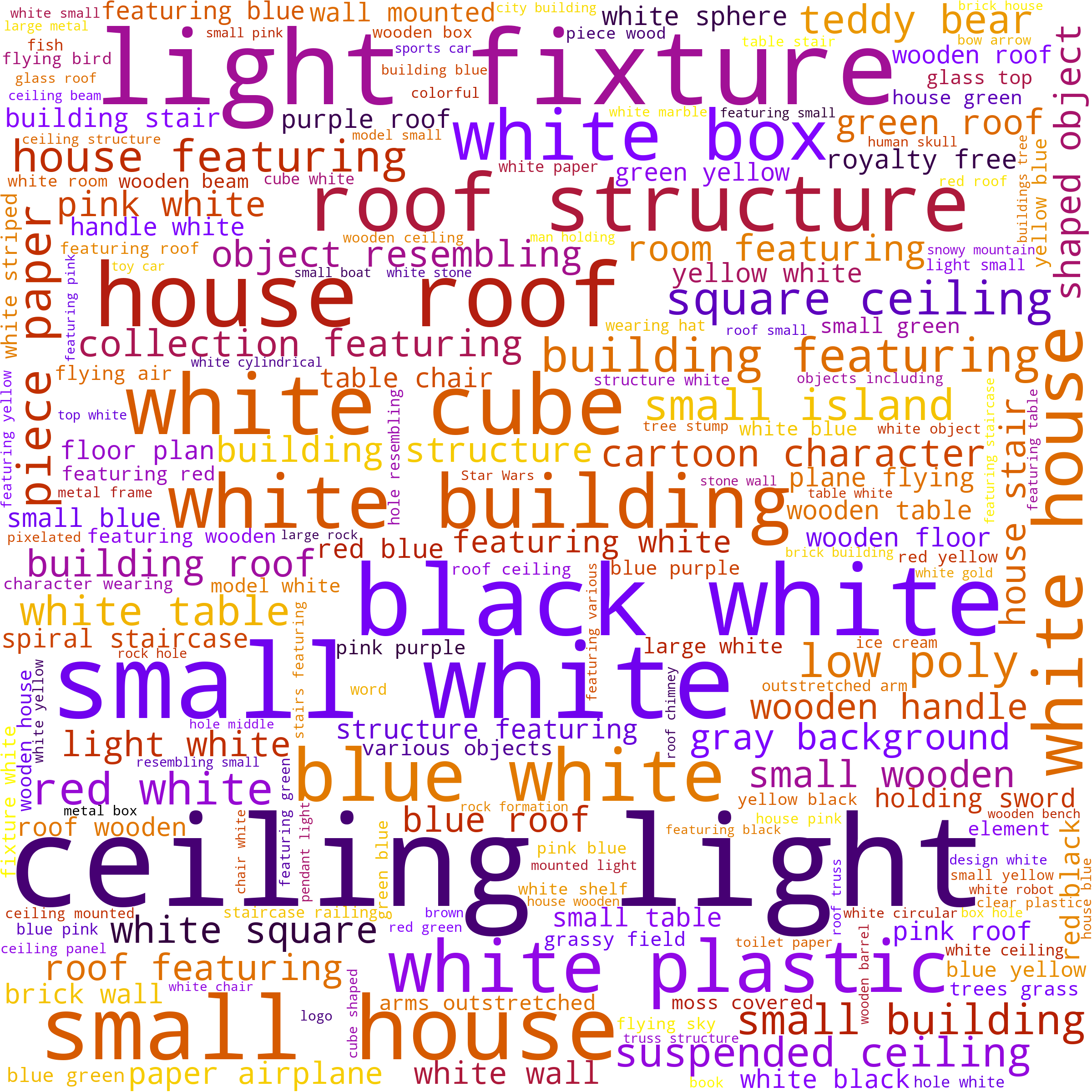
(b) CAP3D aggregate captions.

Figure 8: Word clouds comparing PaLI and CAP3D captions based on word frequency. Articles and prepositions are dropped.

Finally, we plot word frequency clouds in Figure 8 and compute aggregate statistics in Table 4 for both sets of captions. While our pipeline is missing captions for 4% of objects (mostly animations) which we dropped due to rendering issues, CAP3D is missing captions for 17% of Objaverse. CAP3D’s reason for dropping a significant fraction of objects was that they lacked “sufficient camera information for rendering” (see Sec 3.2 of [31]). Nevertheless, both pipelines have better coverage than artist-written tags or descriptions in the original dataset—those are empty for 38% and 37% of all objects respectively.

 

 

 

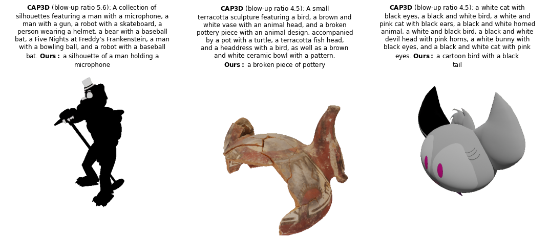
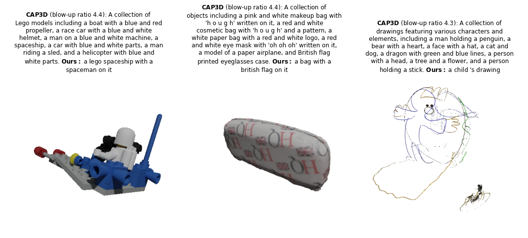
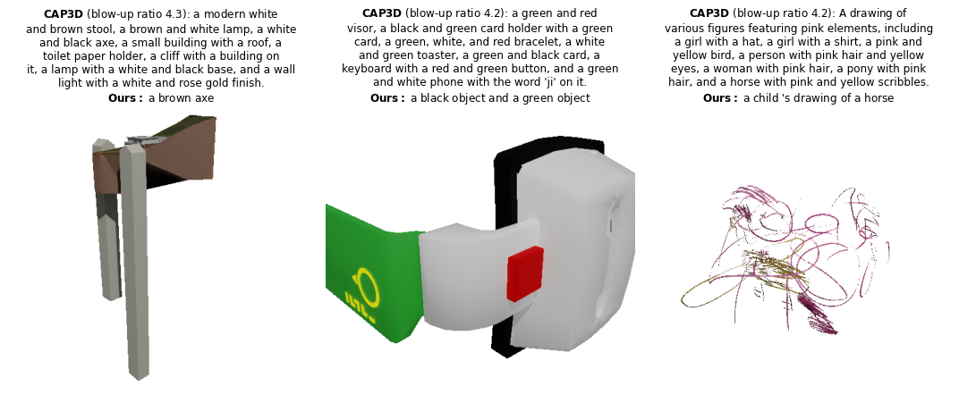
Figure 9: Comparison of view-aggregated captions from our pipeline versus the baseline CAP3D on objects with the highest CAP3D caption blow-up ratios. For CAP3D, we show the no-3D-word post-processed captions.

 

 

 

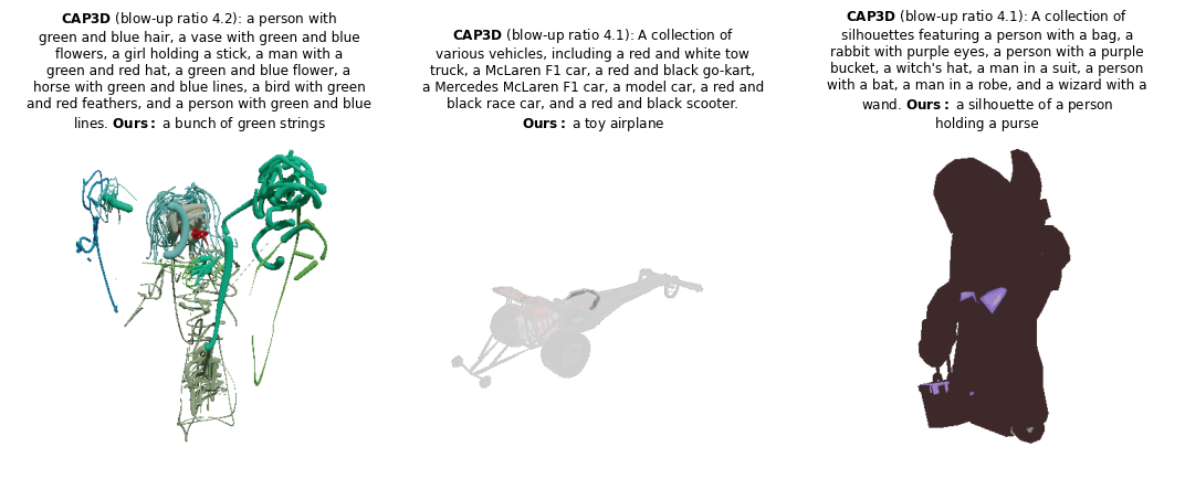
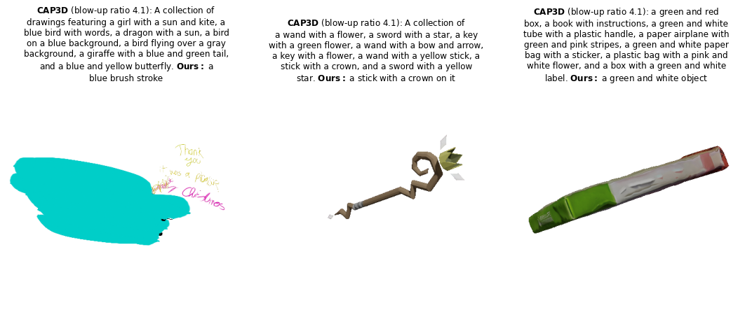
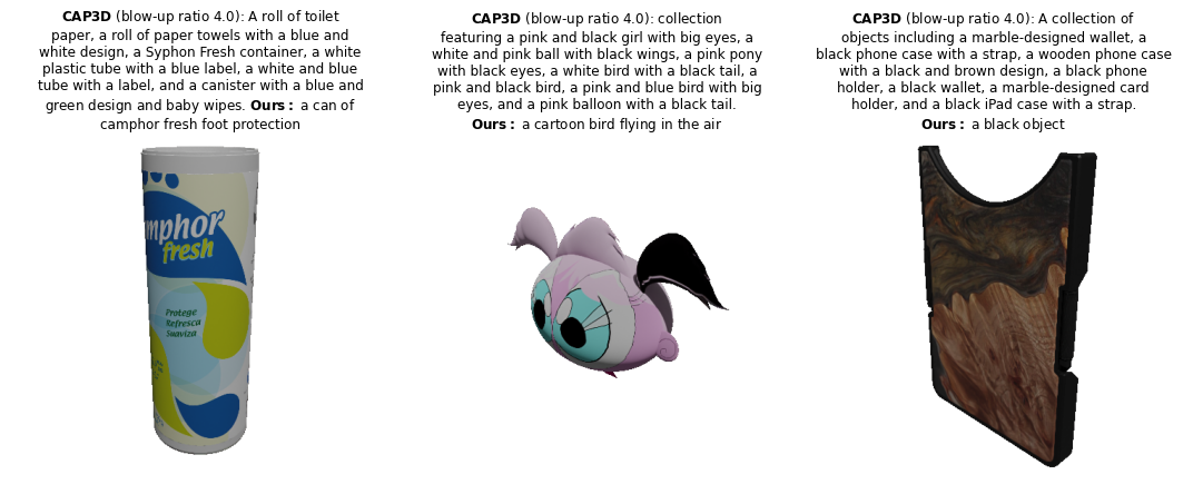
Figure 10: Comparison of view-aggregated captions from our pipeline versus the baseline CAP3D on objects with the highest CAP3D caption blow-up ratios (contd).

 

 

 

 

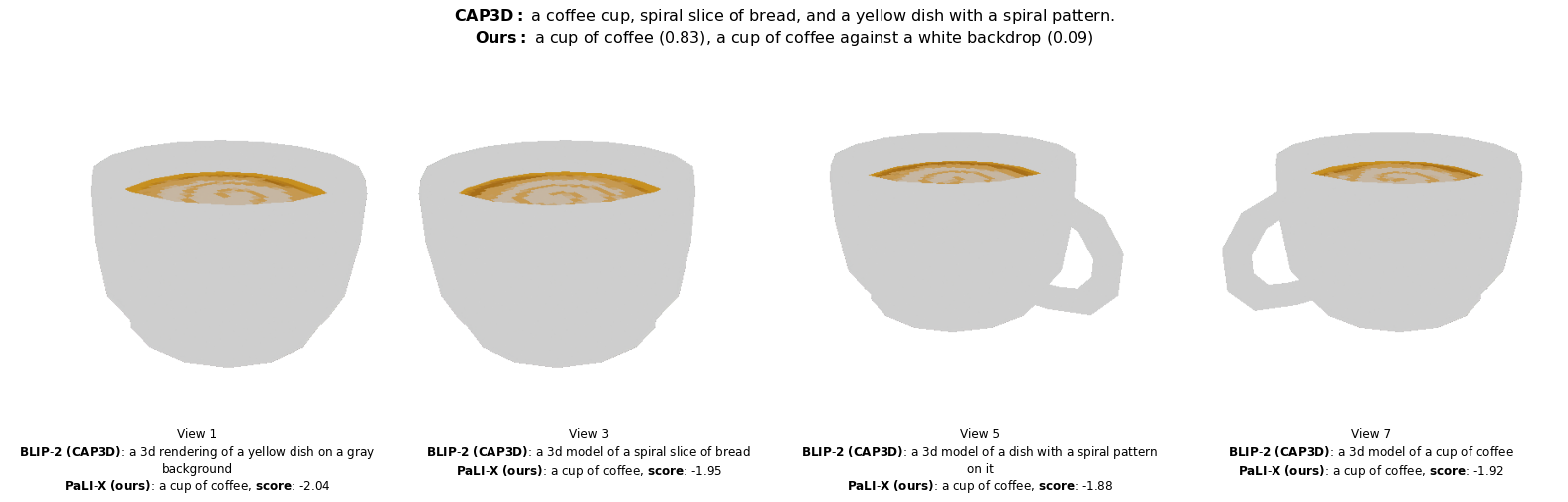
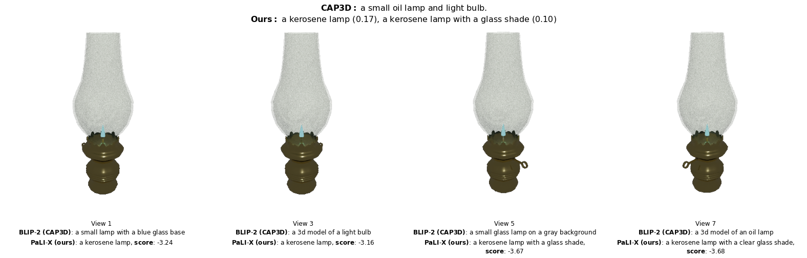
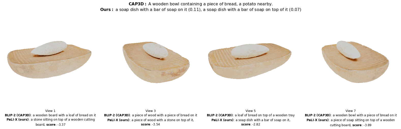
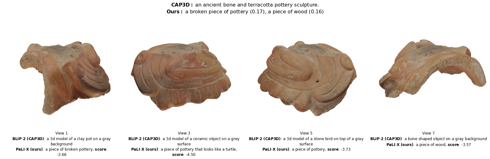
Figure 11: Comparison of captions from our pipeline versus the baseline CAP3D. Besides the aggregates, we also show view-specific captions from the underlying VLMs (PaLI-X and BLIP-2). For CAP3D, we use the no-3D-word post-processed captions.

 

 

 

 

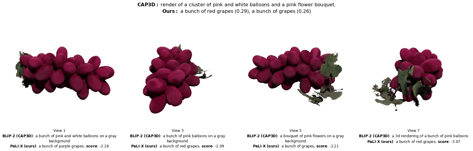
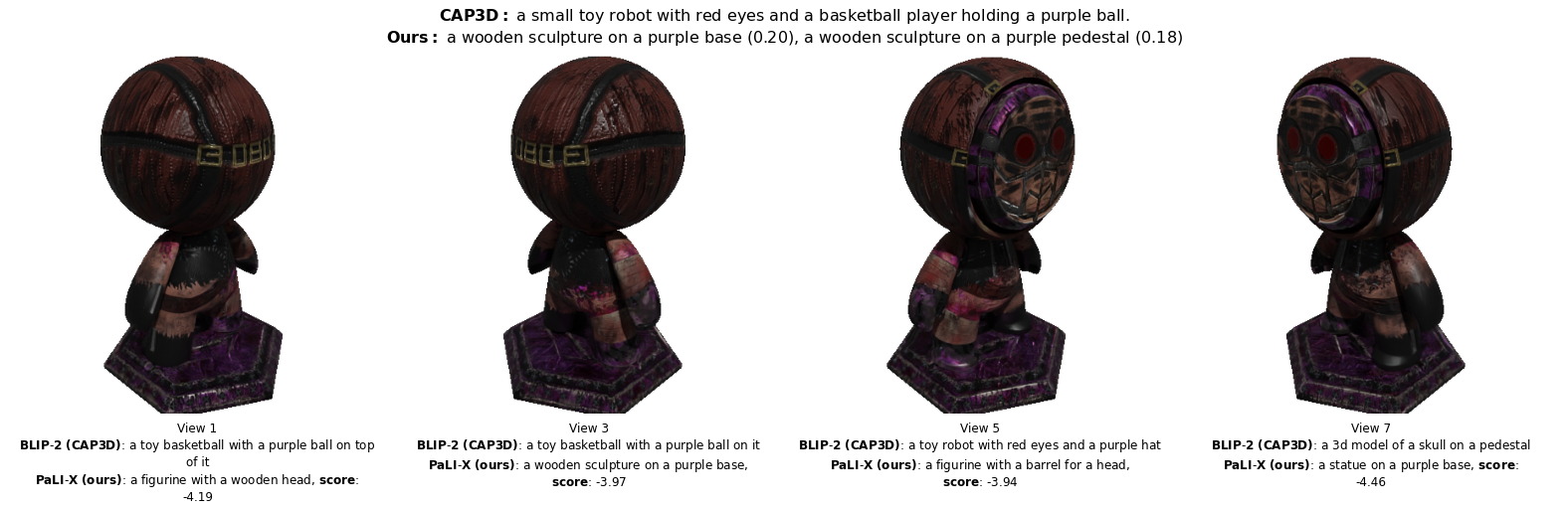
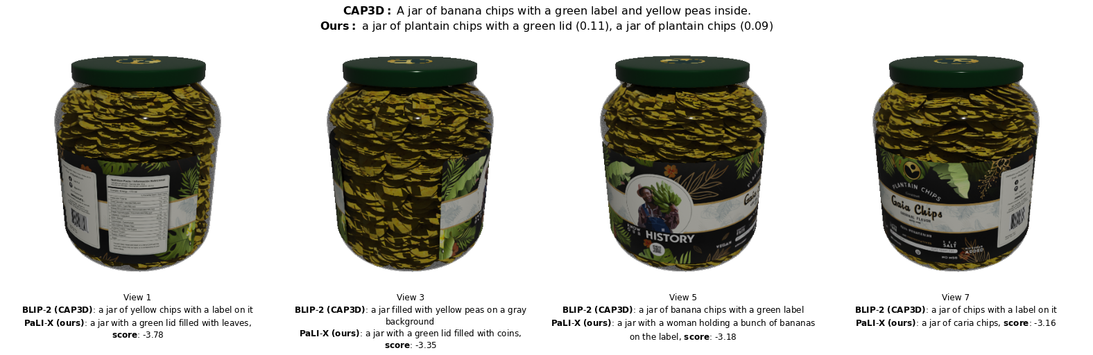
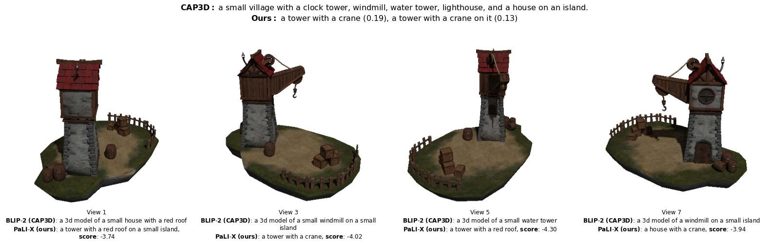
Figure 12: Comparison of captions from our pipeline versus the baseline CAP3D (contd).

 

 

 

 

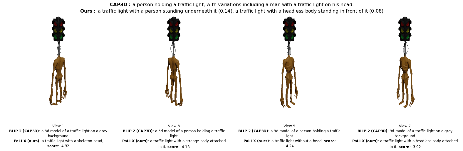
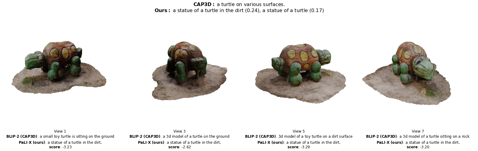
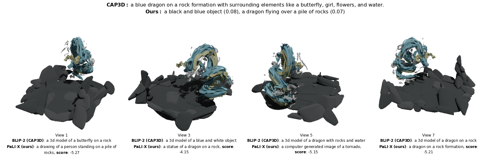
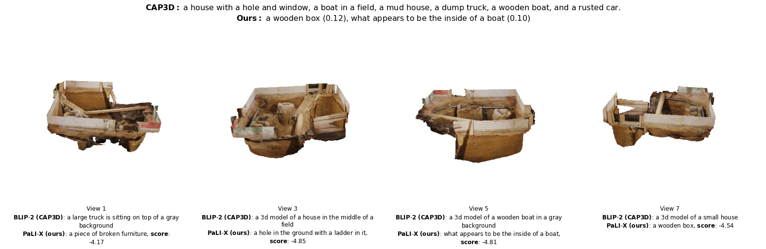
Figure 13: Comparison of captions from our pipeline versus the baseline CAP3D (contd). The last two rows were described as failure cases for CAP3D in that paper.

D.2 Material Inference

We show all material predictions for various objects from our test set in Table LABEL:tab:material_prediction_examples. For aggregate statistics, see Table 1 in the main text.

D.3 What Factors Matter for Different Properties

We take a qualitative look at the effect of varying the question, view, or appearance of an object when predicting various properties. We also observe an effect of object size though we kept it fixed in our pipeline.

First, to examine the role of the question, we fix a set of objects and probe them for all properties discussed so far. We avoid aggregating across object views in this section. For each property we show PaLI responses to question variants separately, plus the single-view aggregate response to show the effect of aggregating across questions. We cover changes in question wording and what prior inferences are specified.

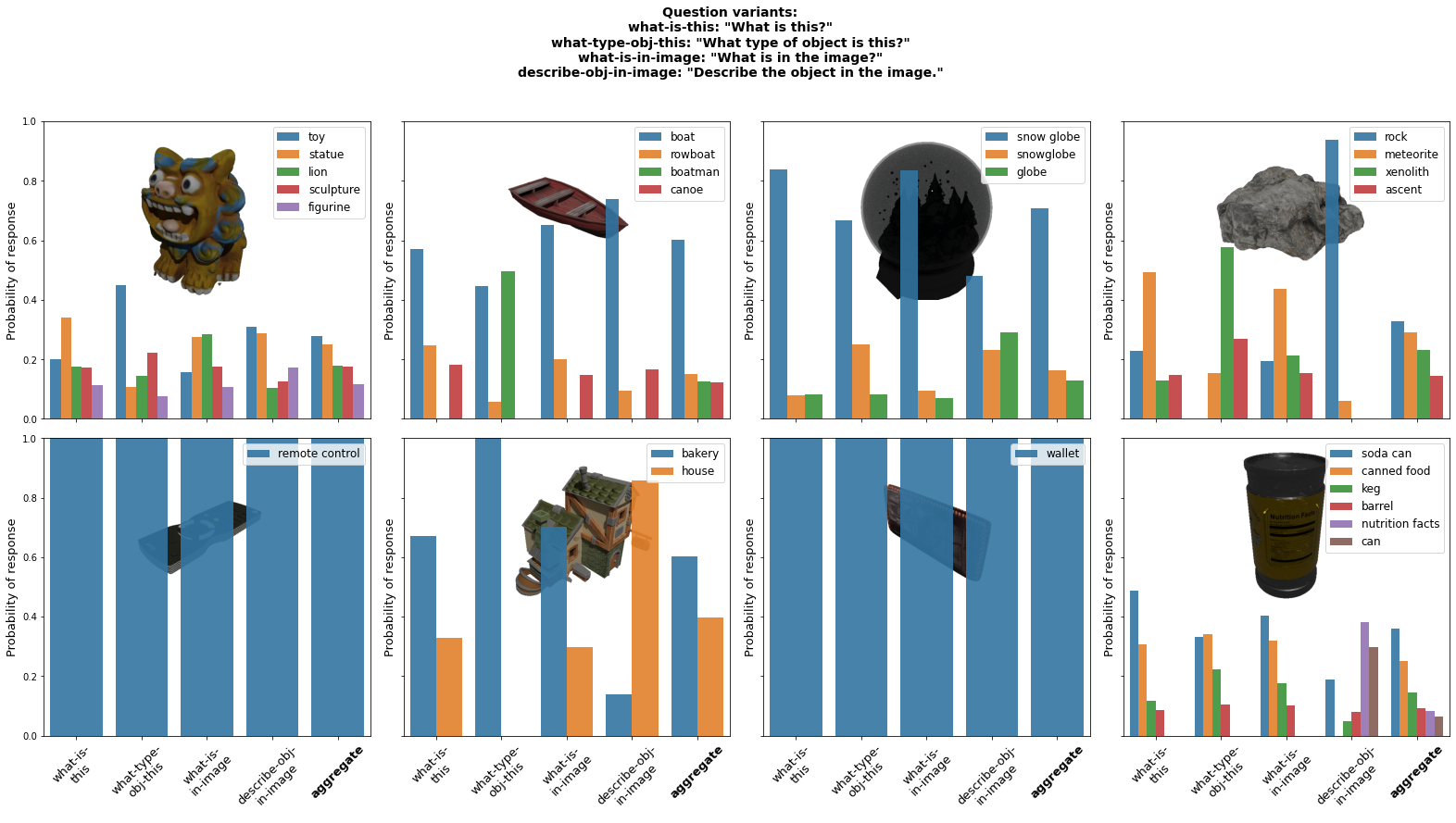
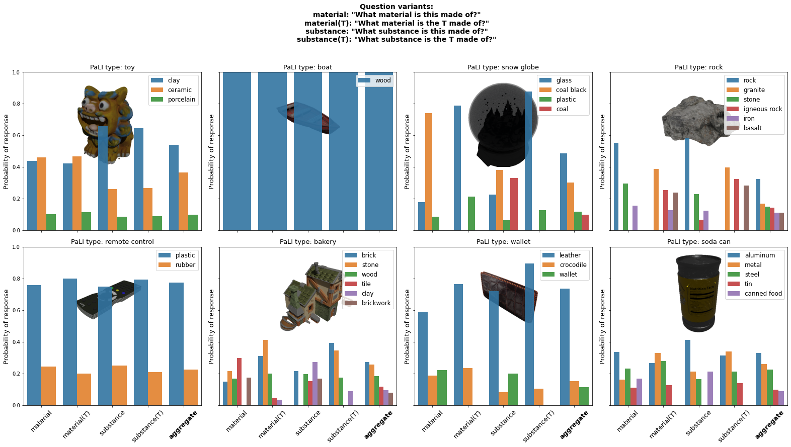
Figure 14: Variations of questions per property for a fixed set of objects. Top: type. Bottom: material.

Open-vocabulary properties. Figure 14 starts with type and material inference. We observe PaLI-X shows varying confidence in its responses on different objects. This could provide signal for when we need to refine predictions (e.g., by asking more questions).

We find PaLI-X surprisingly capable of describing what an object might contain, even when the contained object is hidden or hypothetical (e.g., “money” in a “wallet” or “people” in a “boat”). It is unclear whether the variance across questions here is due to significant changes in wording, or the complexity of the knowledge we’re probing. We ask a single question on object affordance—the space of possible responses and entropy of predictions are large even under a single question. The model appears to understand use cases for all our objects.

Physical behavior. When it comes to physical properties, PaLI makes more mistakes. It knows that a “leather wallet” can be molded but not crushed; that a “brick bakery” would be hard to deform; that a rock can only be crushed. On the other hand, it expects a “wood boat” or “snow globe“ to be moldable by hand. It takes most objects to be fragile (including a “soda can” or “remote control”) and incapable of floating in water (with the obvious exception of a “boat”). Interestingly, whether or not an object contains something significantly changes the likelihood of its floating or sinking.

Lift-ability. When predicting if objects are liftable, we run into the consequences of not controlling for object size. The model is uncertain even in obvious cases like a “clay toy” and “aluminum soda can.” These are both objects for which the height was the maximum dimension; they take up more vertical image space and possibly appear abnormally large to the model. Though we could try aggregating/marginalizing over varying-size renderings of an object, a better solution might specify an object’s scale (if available) to the model explicitly.

Color and count. The model can express colors in words correctly. It offers multi-color responses when there’s a mix of colors (e.g., “yellow and blue” for the clay toy). When it comes to counting, PaLI can separate single objects (count=1) with high precision. It also does reasonably for disjoint objects. For busy scenes, it seems to get the scale right—we even see the variance of its numerical responses increase (e.g. the “banquet”).

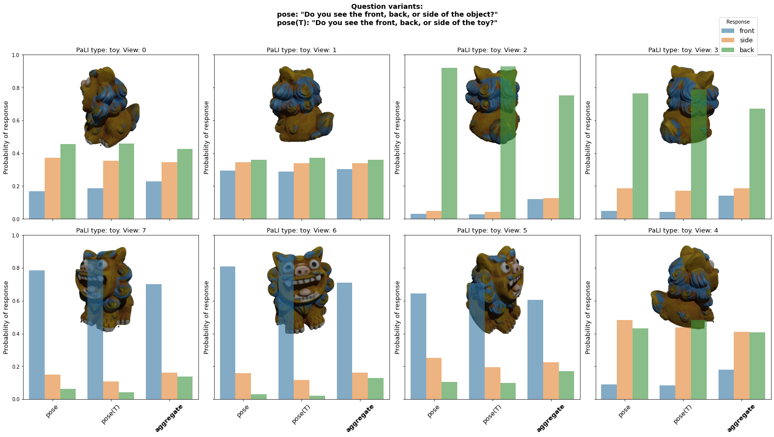
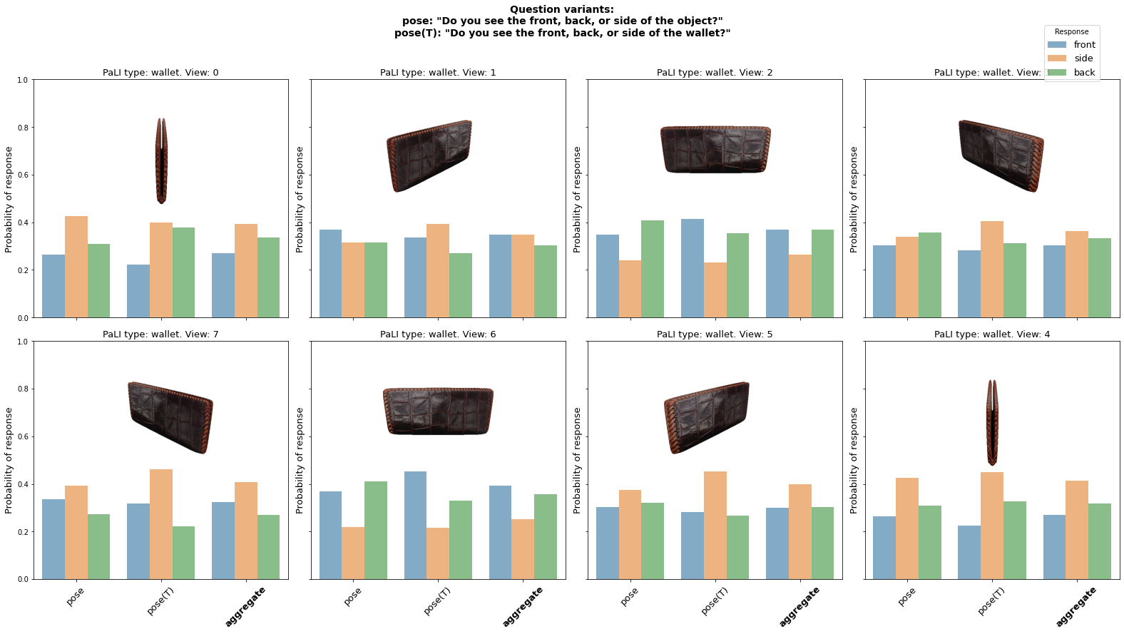
Figure 20: Pose inference. We show eight views per object to the VLM, asking if it knows which side of the object is visible in each view.

Pose. An object appears in different poses to the model across our rendered images (i.e., changes in view). We test whether the model can tell the front of an object from its back or side (Fig 20). This seems readily possible for asymmetric objects, perhaps helped by the presence of facial features in the case of the “lion”. For more symmetrical objects like the “wallet”, the model can tell side views from (squarely) front or back views, but is somewhat confused.

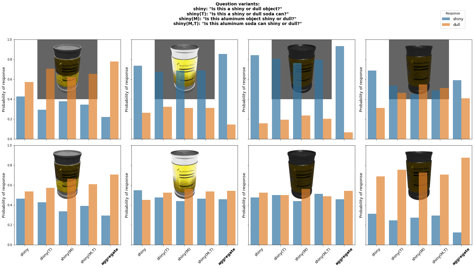
Figure 21: How lighting/rendering settings affect the inference of shininess. For a fixed object, we vary the lighting or camera height across columns, keeping the image background color fixed. The first column uses an area light under the object. The second column uses surround lighting. The third and fourth column use the same camera backlight, but vary in camera height.

Shininess. Whether an object is shiny is a physical property that follows from its type and material. This offers an opportunity to assess whether VLMs are more sensitive to their visual inputs or prompts. We take an object with ambiguous shine, then vary the lighting conditions, camera angle, and background image color (Fig 21). We ask four question variants specifying the object’s type or material in all combinations. We find almost no effect of varying the prompt in comparison to the effect of varying the image settings. The “soda can” is described as shiny and dull in equal measure across the appearance-varying probes.

Conclusion. Running multiple VLM probes and aggregating across them can be a powerful technique to uncover/deal with VLM uncertainty. We can meaningfully marginalize over views of an object (camera pose) or variations in the question. But VLMs can be thrown off by visual features (e.g., lighting, contrast, or object size) especially when they’re not relevant to the query. Such queries should be decoupled from object appearance either by specifying more relevant information in the prompt, or failing that, perhaps using a visionless model.

Table 5: Material prediction examples on 12 categories from our custom test set. We show predicted distributions from both VLMs (PaLI-X and BLIP-2) and all five sets of inputs described in Sec 4. For brevity, only the top two outputs from each predicted distribution are presented, along with their probabilities in parentheses. We use $t_{cap3d}$ or $t_{pali}$ to denote the type annotations, $A$ to denote all object views, $p_{vlm}(\hat{m}|.)$ to denote a predicted distribution, and $m$ to denote the true material.

	$m$	“glass”
	$t_{cap3d}$	“hat and a jar, both with ropes tied around them”
	$t_{pali}$	“potion”
	$p_{pali}(\hat{m}|t_{cap3d})$	“cotton” (0.64), “can’t tell” (0.36)
	$p_{pali}(\hat{m}|t_{pali})$	“potion” (0.35), “glass” (0.27)
	$p_{pali}(\hat{m}|A)$	“cork” (0.45), “glass” (0.19)
	$p_{pali}(\hat{m}|t_{cap3d},A)$	“burlap” (0.44), “canvas” (0.30)
	$p_{pali}(\hat{m}|t_{pali},A)$	“glass” (0.67), “cork” (0.17)
	$p_{blip}(\hat{m}|t_{cap3d})$	“straw” (0.49), “plastic” (0.33)
	$p_{blip}(\hat{m}|t_{pali})$	“a tainted potion made of a tainted potion and a tainted potion” (0.77), “a tainted potion made of a tainted potion, and a tainted poti” (0.14)
	$p_{blip}(\hat{m}|A)$	“wood” (0.83), “rope” (0.10)
	$p_{blip}(\hat{m}|t_{cap3d},A)$	“wood” (0.68), “leather” (0.13)
	$p_{blip}(\hat{m}|t_{pali},A)$	“wood” (0.95), “stone” (0.04)
	$m$	“glass”
	$t_{cap3d}$	“light bulb”
	$t_{pali}$	“light”
	$p_{pali}(\hat{m}|t_{cap3d})$	“glass” (0.77), “filament” (0.11)
	$p_{pali}(\hat{m}|t_{pali})$	“glass” (0.58), “light-emitting diode,LED” (0.13)
	$p_{pali}(\hat{m}|A)$	“glass” (0.41), “brass” (0.19)
	$p_{pali}(\hat{m}|t_{cap3d},A)$	“glass” (0.60), “porcelain” (0.13)
	$p_{pali}(\hat{m}|t_{pali},A)$	“glass” (0.51), “filament” (0.14)
	$p_{blip}(\hat{m}|t_{cap3d})$	“glass” (0.52), “filament” (0.29)
	$p_{blip}(\hat{m}|t_{pali})$	“light-emitting diodes” (0.73), “light-emitting diodes (LEDs)” (0.20)
	$p_{blip}(\hat{m}|A)$	“metal” (0.30), “3ds max” (0.22)
	$p_{blip}(\hat{m}|t_{cap3d},A)$	“metal” (0.84), “gold” (0.13)
	$p_{blip}(\hat{m}|t_{pali},A)$	“metal” (0.78), “gold” (0.14)
	$m$	“porcelain”
	$t_{cap3d}$	“blue and white vase featuring a dragon design”
	$t_{pali}$	“vase”
	$p_{pali}(\hat{m}|t_{cap3d})$	“ceramic” (0.38), “porcelain” (0.34)
	$p_{pali}(\hat{m}|t_{pali})$	“ceramic” (0.35), “glass” (0.31)
	$p_{pali}(\hat{m}|A)$	“faience” (0.62), “porcelain” (0.14)
	$p_{pali}(\hat{m}|t_{cap3d},A)$	“ceramic” (0.38), “porcelain” (0.32)
	$p_{pali}(\hat{m}|t_{pali},A)$	“faience” (0.44), “ceramic” (0.24)
	$p_{blip}(\hat{m}|t_{cap3d})$	“porcelain” (0.65), “Chinese celadon” (0.32)
	$p_{blip}(\hat{m}|t_{pali})$	“Porcelain” (0.86), “terracotta” (0.09)
	$p_{blip}(\hat{m}|A)$	“porcelain” (0.83), “ceramic” (0.08)
	$p_{blip}(\hat{m}|t_{cap3d},A)$	“porcelain” (0.88), “china” (0.12)
	$p_{blip}(\hat{m}|t_{pali},A)$	“porcelain” (0.80), “china” (0.07)
	$m$	“porcelain”
	$t_{cap3d}$	“small white porcelain vase with colorful floral designs on it”
	$t_{pali}$	“inkwell”
	$p_{pali}(\hat{m}|t_{cap3d})$	“porcelain” (0.29), “faience” (0.28)
	$p_{pali}(\hat{m}|t_{pali})$	“glass” (0.28), “porcelain” (0.24)
	$p_{pali}(\hat{m}|A)$	“faience” (0.88), “porcelain” (0.06)
	$p_{pali}(\hat{m}|t_{cap3d},A)$	“faience” (0.68), “porcelain” (0.15)
	$p_{pali}(\hat{m}|t_{pali},A)$	“faience” (0.71), “porcelain” (0.16)
	$p_{blip}(\hat{m}|t_{cap3d})$	“China” (0.58), “ceramic” (0.24)
	$p_{blip}(\hat{m}|t_{pali})$	“metal” (0.93), “metal or plastic” (0.06)
	$p_{blip}(\hat{m}|A)$	“porcelain” (0.99), “white porcelain” (0.01)
	$p_{blip}(\hat{m}|t_{cap3d},A)$	“porcelain” (0.80), “china” (0.12)
	$p_{blip}(\hat{m}|t_{pali},A)$	“porcelain” (0.94), “china” (0.04)
	$m$	“leather”
	$t_{cap3d}$	“armored leather gloves and a brown leather boot”
	$t_{pali}$	“glove”
	$p_{pali}(\hat{m}|t_{cap3d})$	“leather” (0.83), “cowhide” (0.08)
	$p_{pali}(\hat{m}|t_{pali})$	“leather” (0.34), “cotton” (0.21)
	$p_{pali}(\hat{m}|A)$	“leather” (0.69), “armor plate,armour plate,armor plating,plate armor,plate armour” (0.08)
	$p_{pali}(\hat{m}|t_{cap3d},A)$	“leather” (0.80), “cowhide” (0.07)
	$p_{pali}(\hat{m}|t_{pali},A)$	“leather” (0.84), “nylon” (0.04)
	$p_{blip}(\hat{m}|t_{cap3d})$	“leather” (1.00)
	$p_{blip}(\hat{m}|t_{pali})$	“leather” (0.98), “neoprene” (0.02)
	$p_{blip}(\hat{m}|A)$	“leather” (1.00)
	$p_{blip}(\hat{m}|t_{cap3d},A)$	“leather” (1.00), “neoprene” (0.00)
	$p_{blip}(\hat{m}|t_{pali},A)$	“leather” (1.00), “neoprene” (0.00)
	$m$	“leather”
	$t_{cap3d}$	“round tan leather sofa-style dog bed with buttons”
	$t_{pali}$	“dog bed”
	$p_{pali}(\hat{m}|t_{cap3d})$	“leather” (0.70), “suede” (0.16)
	$p_{pali}(\hat{m}|t_{pali})$	“foam” (0.39), “cotton” (0.37)
	$p_{pali}(\hat{m}|A)$	“leather” (0.81), “upholstery” (0.08)
	$p_{pali}(\hat{m}|t_{cap3d},A)$	“leather” (0.87), “faux leather” (0.04)
	$p_{pali}(\hat{m}|t_{pali},A)$	“leather” (0.89), “faux leather” (0.04)
	$p_{blip}(\hat{m}|t_{cap3d})$	“faux leather” (0.87), “faux-leather” (0.13)
	$p_{blip}(\hat{m}|t_{pali})$	“a soft fabric, such as cotton, wool, linen, or a combination of the two” (1.00), “a soft fabric, such as cotton, wool, linen, or a synthetic material, such as acetate or polypropylene” (0.00)
	$p_{blip}(\hat{m}|A)$	“leather” (1.00)
	$p_{blip}(\hat{m}|t_{cap3d},A)$	“leather” (0.79), “3d model” (0.12)
	$p_{blip}(\hat{m}|t_{pali},A)$	“leather” (1.00)
	$m$	“oak”
	$t_{cap3d}$	“wooden staircase with metal railings”
	$t_{pali}$	“bannister”
	$p_{pali}(\hat{m}|t_{cap3d})$	“wood” (0.46), “steel” (0.19)
	$p_{pali}(\hat{m}|t_{pali})$	“wood” (0.80), “marble” (0.07)
	$p_{pali}(\hat{m}|A)$	“wood” (0.78), “timber” (0.06)
	$p_{pali}(\hat{m}|t_{cap3d},A)$	“wood” (0.46), “oak” (0.31)
	$p_{pali}(\hat{m}|t_{pali},A)$	“wood” (0.50), “metal” (0.26)
	$p_{blip}(\hat{m}|t_{cap3d})$	“a wooden staircase with metal railings” (1.00), “a wooden staircase with metal railings is called a balustrade” (0.00)
	$p_{blip}(\hat{m}|t_{pali})$	“wood” (0.73), “wooden” (0.27)
	$p_{blip}(\hat{m}|A)$	“wood” (0.99), “wooden railings” (0.00)
	$p_{blip}(\hat{m}|t_{cap3d},A)$	“wood” (0.98), “wooden staircase with metal railings” (0.02)
	$p_{blip}(\hat{m}|t_{pali},A)$	“wood” (0.97), “wooden” (0.03)
	$m$	“oak”
	$t_{cap3d}$	“small wooden table with two legs and a slanted top”
	$t_{pali}$	“trestle table”
	$p_{pali}(\hat{m}|t_{cap3d})$	“wood” (0.65), “oak” (0.24)
	$p_{pali}(\hat{m}|t_{pali})$	“wood” (0.88), “timber” (0.05)
	$p_{pali}(\hat{m}|A)$	“wood” (0.63), “oak” (0.15)
	$p_{pali}(\hat{m}|t_{cap3d},A)$	“wood” (0.43), “oak” (0.42)
	$p_{pali}(\hat{m}|t_{pali},A)$	“wood” (0.70), “oak” (0.20)
	$p_{blip}(\hat{m}|t_{cap3d})$	“trestle table” (0.80), “a trestle table” (0.20)
	$p_{blip}(\hat{m}|t_{pali})$	“wood” (0.98), “wooden trestle” (0.02)
	$p_{blip}(\hat{m}|A)$	“wood” (0.97), “wooden” (0.03)
	$p_{blip}(\hat{m}|t_{cap3d},A)$	“wood” (0.90), “solid wood” (0.09)
	$p_{blip}(\hat{m}|t_{pali},A)$	“wood” (0.99), “solid wood” (0.01)
	$m$	“metal”
	$t_{cap3d}$	“three-tier metal shelving unit”
	$t_{pali}$	“bookshelf”
	$p_{pali}(\hat{m}|t_{cap3d})$	“steel” (0.41), “metal” (0.29)
	$p_{pali}(\hat{m}|t_{pali})$	“wood” (0.91), “metal” (0.03)
	$p_{pali}(\hat{m}|A)$	“metal” (0.42), “steel” (0.36)
	$p_{pali}(\hat{m}|t_{cap3d},A)$	“steel” (0.49), “metal” (0.29)
	$p_{pali}(\hat{m}|t_{pali},A)$	“metal” (0.59), “steel” (0.20)
	$p_{blip}(\hat{m}|t_{cap3d})$	“steel” (0.99), “steel or stainless steel” (0.01)
	$p_{blip}(\hat{m}|t_{pali})$	“wood” (0.98), “reclaimed wood” (0.02)
	$p_{blip}(\hat{m}|A)$	“metal” (0.72), “steel” (0.21)
	$p_{blip}(\hat{m}|t_{cap3d},A)$	“black metal” (0.43), “steel” (0.32)
	$p_{blip}(\hat{m}|t_{pali},A)$	“metal” (0.68), “steel” (0.20)
	$m$	“metal”
	$t_{cap3d}$	“yellow fire hydrant”
	$t_{pali}$	“fire hydrant”
	$p_{pali}(\hat{m}|t_{cap3d})$	“metal” (0.37), “steel” (0.24)
	$p_{pali}(\hat{m}|t_{pali})$	“metal” (0.32), “steel” (0.25)
	$p_{pali}(\hat{m}|A)$	“iron” (0.31), “metal” (0.17)
	$p_{pali}(\hat{m}|t_{cap3d},A)$	“metal” (0.37), “steel” (0.19)
	$p_{pali}(\hat{m}|t_{pali},A)$	“metal” (0.32), “iron” (0.21)
	$p_{blip}(\hat{m}|t_{cap3d})$	“cast iron” (0.91), “cast-aluminum” (0.09)
	$p_{blip}(\hat{m}|t_{pali})$	“a fire hydrant is a device used to extinguish a fire.” (0.98), “a fire hydrant is a device used to extinguish a fire by means of a pressurized stream of water” (0.01)
	$p_{blip}(\hat{m}|A)$	“plastic” (0.35), “3ds max” (0.24)
	$p_{blip}(\hat{m}|t_{cap3d},A)$	“metal” (0.79), “plastic” (0.20)
	$p_{blip}(\hat{m}|t_{pali},A)$	“metal” (0.70), “plastic” (0.17)
	$m$	“marble”
	$t_{cap3d}$	“white marble column”
	$t_{pali}$	“pedestal”
	$p_{pali}(\hat{m}|t_{cap3d})$	“marble” (0.75), “limestone” (0.09)
	$p_{pali}(\hat{m}|t_{pali})$	“marble” (0.44), “stone” (0.31)
	$p_{pali}(\hat{m}|A)$	“marble” (0.69), “stone” (0.17)
	$p_{pali}(\hat{m}|t_{cap3d},A)$	“marble” (0.73), “carrara” (0.10)
	$p_{pali}(\hat{m}|t_{pali},A)$	“marble” (0.67), “stone” (0.21)
	$p_{blip}(\hat{m}|t_{cap3d})$	“marble” (1.00)
	$p_{blip}(\hat{m}|t_{pali})$	“marble” (1.00)
	$p_{blip}(\hat{m}|A)$	“marble” (0.96), “wood” (0.04)
	$p_{blip}(\hat{m}|t_{cap3d},A)$	“marble” (0.73), “white marble” (0.27)
	$p_{blip}(\hat{m}|t_{pali},A)$	“marble” (0.95), “wood” (0.04)
	$m$	“marble”
	$t_{cap3d}$	“white marble skull”
	$t_{pali}$	“skull”
	$p_{pali}(\hat{m}|t_{cap3d})$	“marble” (0.79), “porcelain” (0.09)
	$p_{pali}(\hat{m}|t_{pali})$	“bone” (0.75), “bones” (0.09)
	$p_{pali}(\hat{m}|A)$	“clay” (0.35), “marble” (0.22)
	$p_{pali}(\hat{m}|t_{cap3d},A)$	“marble” (0.55), “clay” (0.20)
	$p_{pali}(\hat{m}|t_{pali},A)$	“clay” (0.33), “marble” (0.27)
	$p_{blip}(\hat{m}|t_{cap3d})$	“limestone” (0.68), “marble” (0.32)
	$p_{blip}(\hat{m}|t_{pali})$	“calcium phosphate” (0.83), “calcareous limestone” (0.08)
	$p_{blip}(\hat{m}|A)$	“marble” (0.81), “white marble” (0.10)
	$p_{blip}(\hat{m}|t_{cap3d},A)$	“white marble” (0.85), “marble” (0.07)
	$p_{blip}(\hat{m}|t_{pali},A)$	“marble” (0.43), “limestone” (0.36)
	$m$	“wood”
	$t_{cap3d}$	“small metal house with a roof and legs”
	$t_{pali}$	“birdhouse”
	$p_{pali}(\hat{m}|t_{cap3d})$	“aluminum” (0.48), “steel” (0.34)
	$p_{pali}(\hat{m}|t_{pali})$	“wood” (0.75), “clay” (0.10)
	$p_{pali}(\hat{m}|A)$	“wood” (0.42), “copper” (0.23)
	$p_{pali}(\hat{m}|t_{cap3d},A)$	“steel” (0.21), “iron” (0.19)
	$p_{pali}(\hat{m}|t_{pali},A)$	“wood” (0.61), “metal” (0.17)
	$p_{blip}(\hat{m}|t_{cap3d})$	“a styrofoam styrofoam styrofoam sty” (0.36), “a styrofoam styrofoam styrofoam sandwich” (0.33)
	$p_{blip}(\hat{m}|t_{pali})$	“wood” (0.68), “Cedar” (0.31)
	$p_{blip}(\hat{m}|A)$	“metal” (0.86), “wood” (0.07)
	$p_{blip}(\hat{m}|t_{cap3d},A)$	“3d model” (0.59), “rusty metal” (0.21)
	$p_{blip}(\hat{m}|t_{pali},A)$	“metal” (0.61), “wood” (0.33)
	$m$	“wood”
	$t_{cap3d}$	“wooden rocking chair”
	$t_{pali}$	“rocking chair”
	$p_{pali}(\hat{m}|t_{cap3d})$	“wood” (0.58), “oak” (0.22)
	$p_{pali}(\hat{m}|t_{pali})$	“wood” (0.81), “wicker” (0.08)
	$p_{pali}(\hat{m}|A)$	“wood” (0.88), “rattan” (0.04)
	$p_{pali}(\hat{m}|t_{cap3d},A)$	“oak” (0.40), “wood” (0.22)
	$p_{pali}(\hat{m}|t_{pali},A)$	“wood” (0.93), “mahogany” (0.02)
	$p_{blip}(\hat{m}|t_{cap3d})$	“wood” (0.96), “rattan” (0.04)
	$p_{blip}(\hat{m}|t_{pali})$	“wood” (0.97), “wooden rocking chair” (0.03)
	$p_{blip}(\hat{m}|A)$	“wood” (0.98), “wooden” (0.01)
	$p_{blip}(\hat{m}|t_{cap3d},A)$	“wood” (0.96), “wooden rocking chair” (0.04)
	$p_{blip}(\hat{m}|t_{pali},A)$	“wood” (1.00), “wooden rocking chair” (0.00)
	$m$	“ceramic”
	$t_{cap3d}$	“terracotta bowl with a curved top, flat bottom”
	$t_{pali}$	“tray”
	$p_{pali}(\hat{m}|t_{cap3d})$	“ceramic” (0.40), “stoneware” (0.25)
	$p_{pali}(\hat{m}|t_{pali})$	“wood” (0.28), “ceramic” (0.24)
	$p_{pali}(\hat{m}|A)$	“clay” (0.33), “stoneware” (0.28)
	$p_{pali}(\hat{m}|t_{cap3d},A)$	“clay” (0.47), “ceramic” (0.18)
	$p_{pali}(\hat{m}|t_{pali},A)$	“clay” (0.41), “stoneware” (0.19)
	$p_{blip}(\hat{m}|t_{cap3d})$	“earthenware” (0.55), “terracotta” (0.31)
	$p_{blip}(\hat{m}|t_{pali})$	“stainless steel” (1.00), “stainless steel or stainless steel-alloys” (0.00)
	$p_{blip}(\hat{m}|A)$	“clay” (0.92), “terracotta” (0.05)
	$p_{blip}(\hat{m}|t_{cap3d},A)$	“clay” (0.64), “terracotta” (0.35)
	$p_{blip}(\hat{m}|t_{pali},A)$	“clay” (0.94), “terracotta” (0.05)
	$m$	“ceramic”
	$t_{cap3d}$	“vase with two handles and intricate designs”
	$t_{pali}$	“jug”
	$p_{pali}(\hat{m}|t_{cap3d})$	“ceramic” (0.38), “porcelain” (0.27)
	$p_{pali}(\hat{m}|t_{pali})$	“glass” (0.56), “porcelain” (0.17)
	$p_{pali}(\hat{m}|A)$	“stoneware” (0.29), “clay” (0.23)
	$p_{pali}(\hat{m}|t_{cap3d},A)$	“clay” (0.36), “pottery” (0.27)
	$p_{pali}(\hat{m}|t_{pali},A)$	“ceramic” (0.29), “clay” (0.27)
	$p_{blip}(\hat{m}|t_{cap3d})$	“Chinese celadon” (0.97), “Chinese lacquerware” (0.02)
	$p_{blip}(\hat{m}|t_{pali})$	“clay” (0.87), “tin” (0.13)
	$p_{blip}(\hat{m}|A)$	“clay” (0.73), “ceramic” (0.27)
	$p_{blip}(\hat{m}|t_{cap3d},A)$	“clay” (0.76), “ceramic” (0.24)
	$p_{blip}(\hat{m}|t_{pali},A)$	“clay” (0.87), “ceramic” (0.13)
	$m$	“gold”
	$t_{cap3d}$	“gold flower ring featuring a yellow and white flower design”
	$t_{pali}$	“hair slide”
	$p_{pali}(\hat{m}|t_{cap3d})$	“gold” (0.74), “sterling silver” (0.09)
	$p_{pali}(\hat{m}|t_{pali})$	“plastic” (0.44), “rubber” (0.24)
	$p_{pali}(\hat{m}|A)$	“gold plate” (0.33), “brass” (0.31)
	$p_{pali}(\hat{m}|t_{cap3d},A)$	“gold” (0.40), “brass” (0.24)
	$p_{pali}(\hat{m}|t_{pali},A)$	“brass” (0.23), “metal” (0.23)
	$p_{blip}(\hat{m}|t_{cap3d})$	“14K yellow gold” (0.35), “18k white gold” (0.34)
	$p_{blip}(\hat{m}|t_{pali})$	“plastic” (0.88), “acetate” (0.12)
	$p_{blip}(\hat{m}|A)$	“gold” (0.65), “metal” (0.32)
	$p_{blip}(\hat{m}|t_{cap3d},A)$	“gold” (0.59), “3d model” (0.15)
	$p_{blip}(\hat{m}|t_{pali},A)$	“gold” (0.72), “metal” (0.22)
	$m$	“gold”
	$t_{cap3d}$	“gold Egyptian cat ring”
	$t_{pali}$	“ring”
	$p_{pali}(\hat{m}|t_{cap3d})$	“gold” (0.68), “gold plate” (0.11)
	$p_{pali}(\hat{m}|t_{pali})$	“gold” (0.74), “brass” (0.10)
	$p_{pali}(\hat{m}|A)$	“gold” (0.63), “gold plate” (0.20)
	$p_{pali}(\hat{m}|t_{cap3d},A)$	“gold” (0.78), “brass” (0.10)
	$p_{pali}(\hat{m}|t_{pali},A)$	“gold” (0.82), “brass” (0.09)
	$p_{blip}(\hat{m}|t_{cap3d})$	“gold” (1.00), “gold-plated tibetan calfskin” (0.00)
	$p_{blip}(\hat{m}|t_{pali})$	“precious metals, such as gold, silver, platinum, palladium, and rhodium” (0.93), “precious metals, such as gold, silver, platinum, palladium, rhodium, and tin” (0.03)
	$p_{blip}(\hat{m}|A)$	“gold” (1.00), “gold 3d printed” (0.00)
	$p_{blip}(\hat{m}|t_{cap3d},A)$	“gold” (0.90), “3d printed” (0.10)
	$p_{blip}(\hat{m}|t_{pali},A)$	“gold” (1.00)
	$m$	“rubber”
	$t_{cap3d}$	“tire”
	$t_{pali}$	“tire”
	$p_{pali}(\hat{m}|t_{cap3d})$	“rubber” (0.99), “rubber and steel” (0.00)
	$p_{pali}(\hat{m}|t_{pali})$	“rubber” (0.99), “rubber and steel” (0.00)
	$p_{pali}(\hat{m}|A)$	“rubber” (0.96), “blacktop,blacktopping” (0.02)
	$p_{pali}(\hat{m}|t_{cap3d},A)$	“rubber” (0.97), “black rubber” (0.01)
	$p_{pali}(\hat{m}|t_{pali},A)$	“rubber” (0.97), “black rubber” (0.01)
	$p_{blip}(\hat{m}|t_{cap3d})$	“rubber” (0.90), “pneumatic tires” (0.09)
	$p_{blip}(\hat{m}|t_{pali})$	“rubber” (0.73), “Rubber” (0.27)
	$p_{blip}(\hat{m}|A)$	“rubber” (0.87), “black rubber” (0.10)
	$p_{blip}(\hat{m}|t_{cap3d},A)$	“rubber” (0.93), “black rubber” (0.06)
	$p_{blip}(\hat{m}|t_{pali},A)$	“rubber” (0.91), “black rubber” (0.09)
	$m$	“rubber”
	$t_{cap3d}$	“green coiled cable with a white plug and attached earbud”
	$t_{pali}$	“hose”
	$p_{pali}(\hat{m}|t_{cap3d})$	“nylon” (0.44), “plastic” (0.36)
	$p_{pali}(\hat{m}|t_{pali})$	“rubber” (0.86), “plastic” (0.05)
	$p_{pali}(\hat{m}|A)$	“hose” (0.48), “rubber” (0.20)
	$p_{pali}(\hat{m}|t_{cap3d},A)$	“rubber” (0.38), “plastic” (0.19)
	$p_{pali}(\hat{m}|t_{pali},A)$	“rubber” (0.70), “plastic” (0.15)
	$p_{blip}(\hat{m}|t_{cap3d})$	“tin-alloy” (0.79), “tin-plated copper” (0.20)
	$p_{blip}(\hat{m}|t_{pali})$	“rubber” (0.95), “PTFE” (0.05)
	$p_{blip}(\hat{m}|A)$	“wire” (0.33), “metal” (0.26)
	$p_{blip}(\hat{m}|t_{cap3d},A)$	“teflon” (0.92), “stranded copper” (0.05)
	$p_{blip}(\hat{m}|t_{pali},A)$	“plastic” (0.36), “pvc” (0.23)
	$m$	“cardboard”
	$t_{cap3d}$	“stack of brown cardboard boxes with white tape on them”
	$t_{pali}$	“packing box”
	$p_{pali}(\hat{m}|t_{cap3d})$	“cardboard” (0.64), “paper” (0.30)
	$p_{pali}(\hat{m}|t_{pali})$	“cardboard” (0.74), “paper” (0.13)
	$p_{pali}(\hat{m}|A)$	“cardboard” (0.52), “cellulose tape,Scotch tape,Sellotape” (0.17)
	$p_{pali}(\hat{m}|t_{cap3d},A)$	“cardboard” (0.67), “paper” (0.13)
	$p_{pali}(\hat{m}|t_{pali},A)$	“cardboard” (0.82), “corrugated cardboard” (0.06)
	$p_{blip}(\hat{m}|t_{cap3d})$	“shipping cartons” (1.00), “a receptacle for the shipment of goods” (0.00)
	$p_{blip}(\hat{m}|t_{pali})$	“cardboard” (0.65), “paper” (0.27)
	$p_{blip}(\hat{m}|A)$	“cardboard” (1.00), “styrofoam” (0.00)
	$p_{blip}(\hat{m}|t_{cap3d},A)$	“cardboard” (0.96), “3d model” (0.01)
	$p_{blip}(\hat{m}|t_{pali},A)$	“cardboard” (0.99), “paper” (0.01)
	$m$	“cardboard”
	$t_{cap3d}$	“cardboard Amazon robot toy with logo”
	$t_{pali}$	“carton”
	$p_{pali}(\hat{m}|t_{cap3d})$	“cardboard” (0.57), “paper” (0.32)
	$p_{pali}(\hat{m}|t_{pali})$	“cardboard” (0.47), “paper” (0.45)
	$p_{pali}(\hat{m}|A)$	“cardboard” (0.80), “carton” (0.13)
	$p_{pali}(\hat{m}|t_{cap3d},A)$	“cardboard” (0.73), “carton” (0.10)
	$p_{pali}(\hat{m}|t_{pali},A)$	“cardboard” (0.85), “corrugated cardboard” (0.06)
	$p_{blip}(\hat{m}|t_{cap3d})$	“cardboard” (0.99), “acetate” (0.01)
	$p_{blip}(\hat{m}|t_{pali})$	“paper” (0.75), “paperboard” (0.25)
	$p_{blip}(\hat{m}|A)$	“cardboard” (1.00)
	$p_{blip}(\hat{m}|t_{cap3d},A)$	“cardboard” (1.00), “cardboard, cardboard boxes, cardboard boxes, cardboard boxes, cardboard boxes, cardboard boxes, cardboard boxes, cardboard boxes, cardboard boxes, cardboard boxes, cardboard” (0.00)
	$p_{blip}(\hat{m}|t_{pali},A)$	“cardboard” (0.99), “paper” (0.01)
	$m$	“plastic”
	$t_{cap3d}$	“large silver trash bag”
	$t_{pali}$	“garbage bag”
	$p_{pali}(\hat{m}|t_{cap3d})$	“plastic” (0.45), “aluminum” (0.35)
	$p_{pali}(\hat{m}|t_{pali})$	“plastic” (0.80), “polythene” (0.07)
	$p_{pali}(\hat{m}|A)$	“garbage” (0.45), “plastic” (0.42)
	$p_{pali}(\hat{m}|t_{cap3d},A)$	“plastic” (0.66), “cellophane” (0.13)
	$p_{pali}(\hat{m}|t_{pali},A)$	“plastic” (0.83), “polythene” (0.06)
	$p_{blip}(\hat{m}|t_{cap3d})$	“plastic” (0.97), “woven polypropylene” (0.03)
	$p_{blip}(\hat{m}|t_{pali})$	“plastic” (1.00), “a polyethylene terephthalate (PET) film” (0.00)
	$p_{blip}(\hat{m}|A)$	“black plastic” (0.67), “3ds max” (0.15)
	$p_{blip}(\hat{m}|t_{cap3d},A)$	“plastic” (0.83), “black plastic” (0.11)
	$p_{blip}(\hat{m}|t_{pali},A)$	“plastic” (0.60), “black plastic” (0.38)
	$m$	“plastic”
	$t_{cap3d}$	“blue plastic bowl with a lid”
	$t_{pali}$	“washtub”
	$p_{pali}(\hat{m}|t_{cap3d})$	“polypropylene” (0.53), “plastic” (0.47)
	$p_{pali}(\hat{m}|t_{pali})$	“porcelain” (0.56), “ceramic” (0.35)
	$p_{pali}(\hat{m}|A)$	“plastic” (0.65), “polypropylene” (0.18)
	$p_{pali}(\hat{m}|t_{cap3d},A)$	“polypropylene” (0.58), “plastic” (0.24)
	$p_{pali}(\hat{m}|t_{pali},A)$	“plastic” (0.78), “polypropylene” (0.10)
	$p_{blip}(\hat{m}|t_{cap3d})$	“borosilicate glass” (0.97), “PP (Polypropylene)” (0.02)
	$p_{blip}(\hat{m}|t_{pali})$	“plastic” (0.90), “tin” (0.10)
	$p_{blip}(\hat{m}|A)$	“plastic” (1.00), “polygons” (0.00)
	$p_{blip}(\hat{m}|t_{cap3d},A)$	“plastic” (0.99), “polypropylene” (0.01)
	$p_{blip}(\hat{m}|t_{pali},A)$	“plastic” (1.00)

 

 

 

 

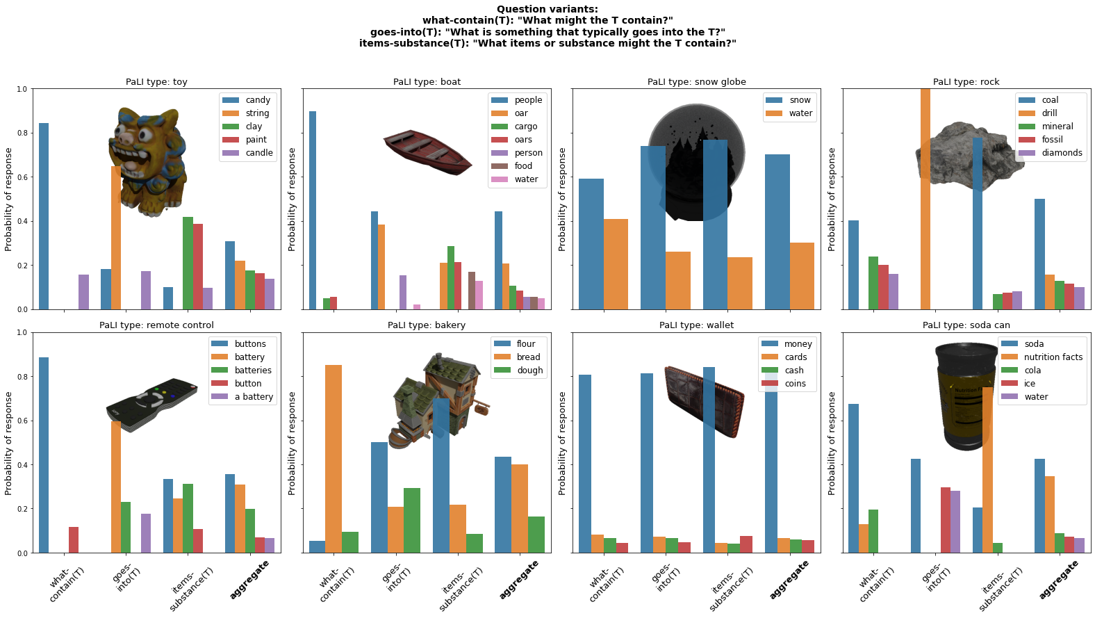
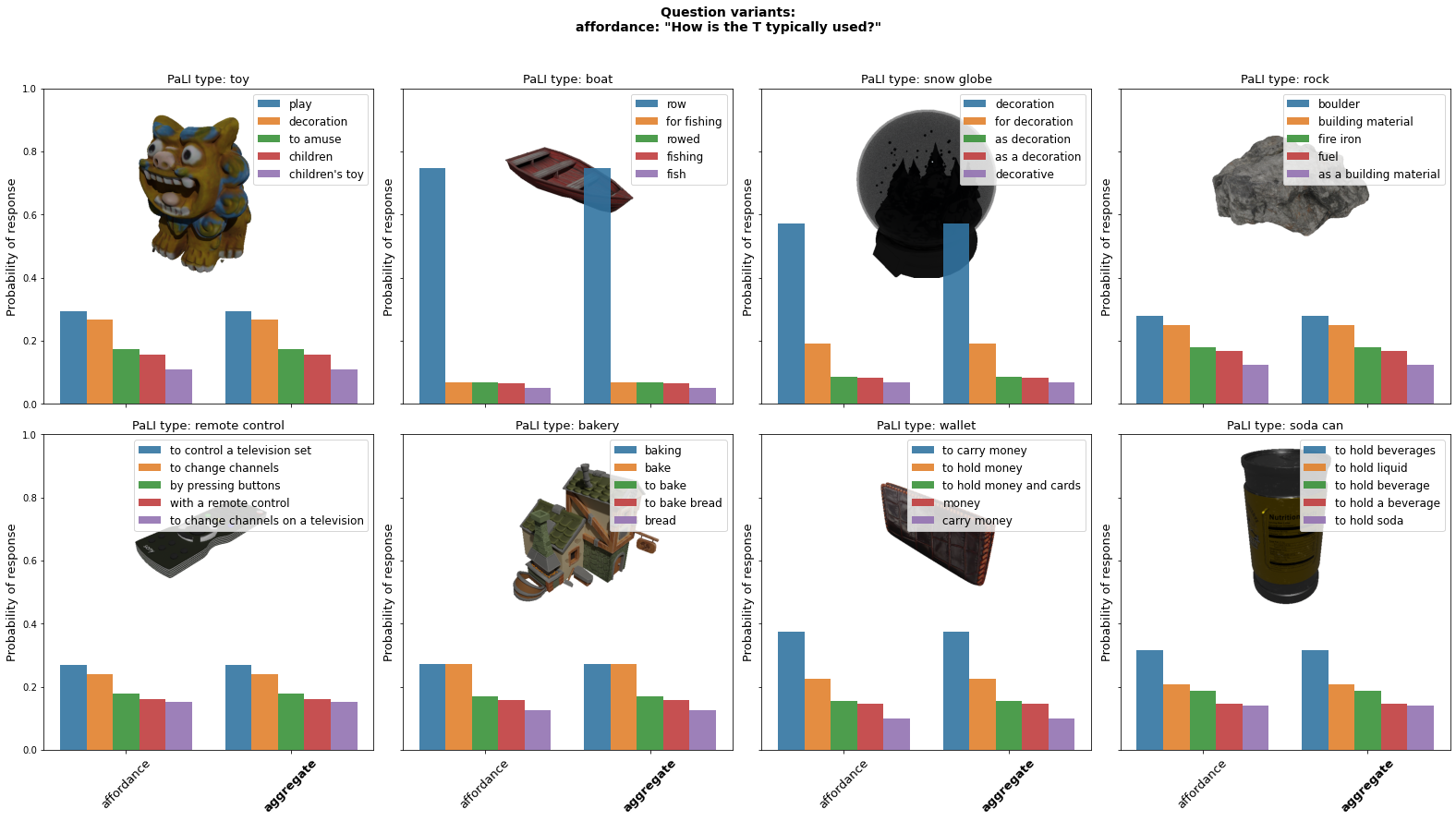
Figure 15: Variations of questions per property for a fixed set of objects (contd). Top: containment. Bottom: affordance.

 

 

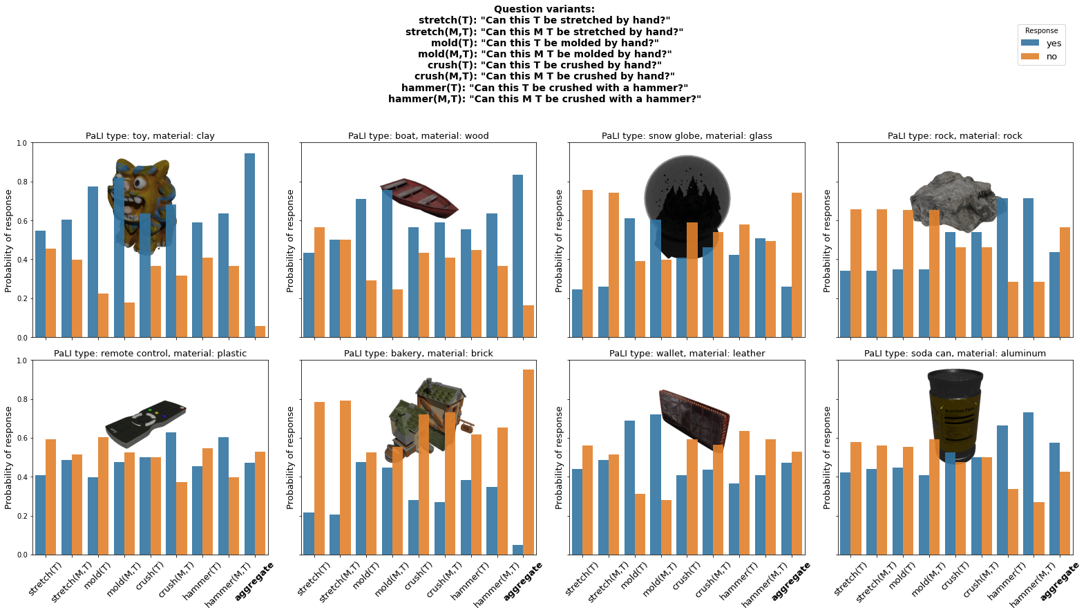
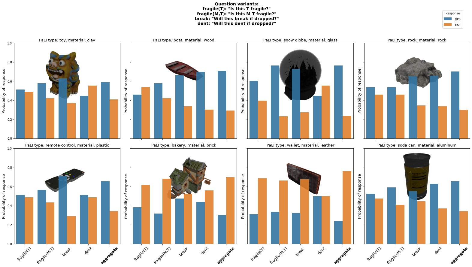
Figure 16: Variations of questions per property for a fixed set of objects (contd). Top: deformability. Bottom: fragility.

 

 

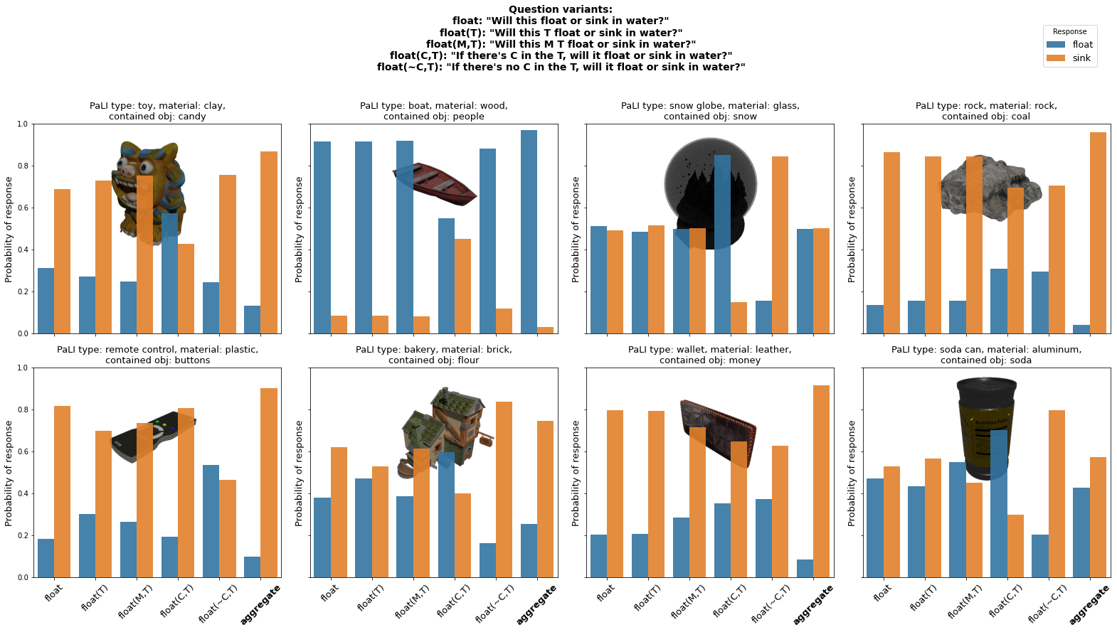
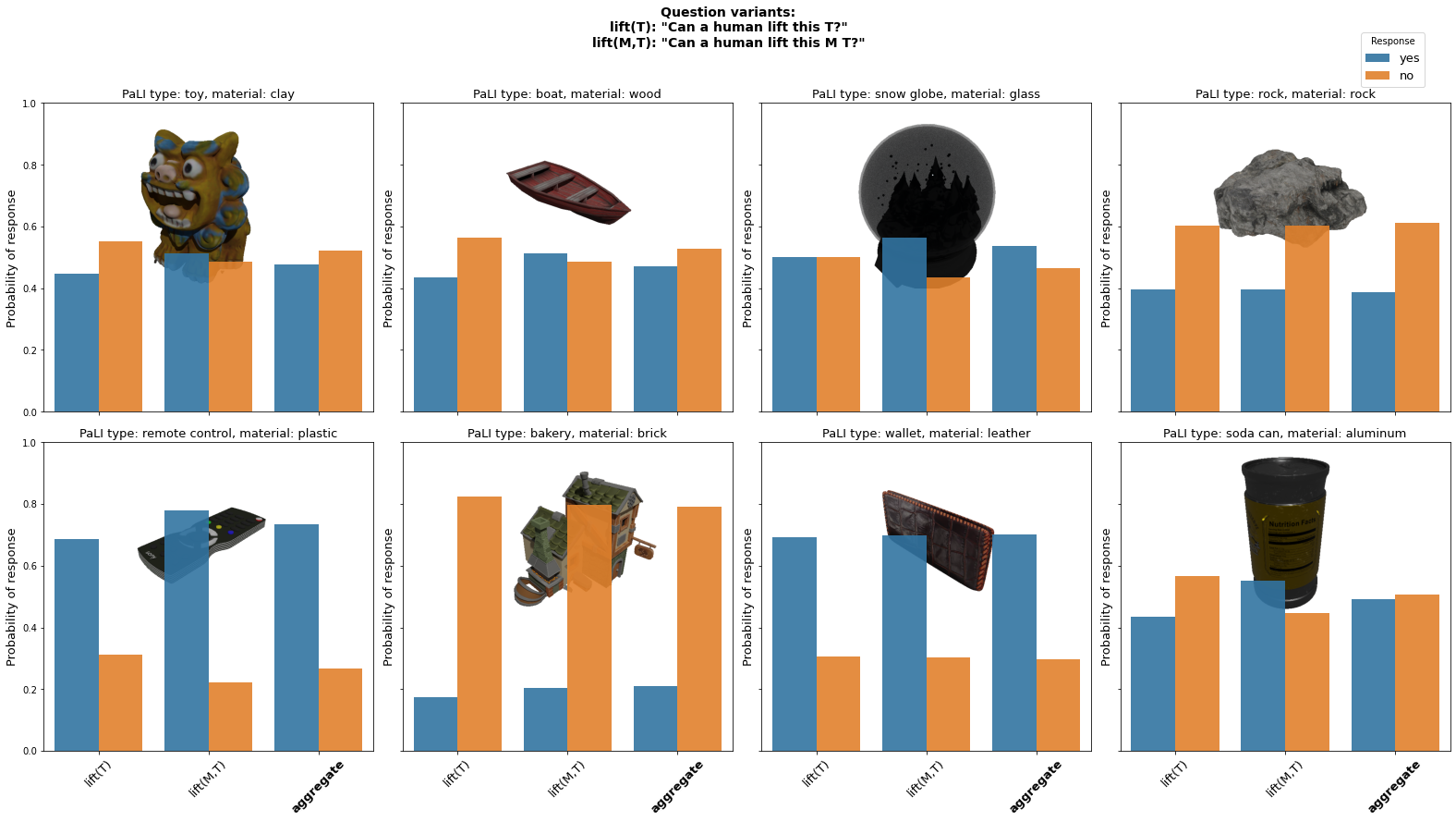
Figure 17: Variations of questions per property for a fixed set of objects (contd). Top: float-ability. Bottom: lift-ability.

 

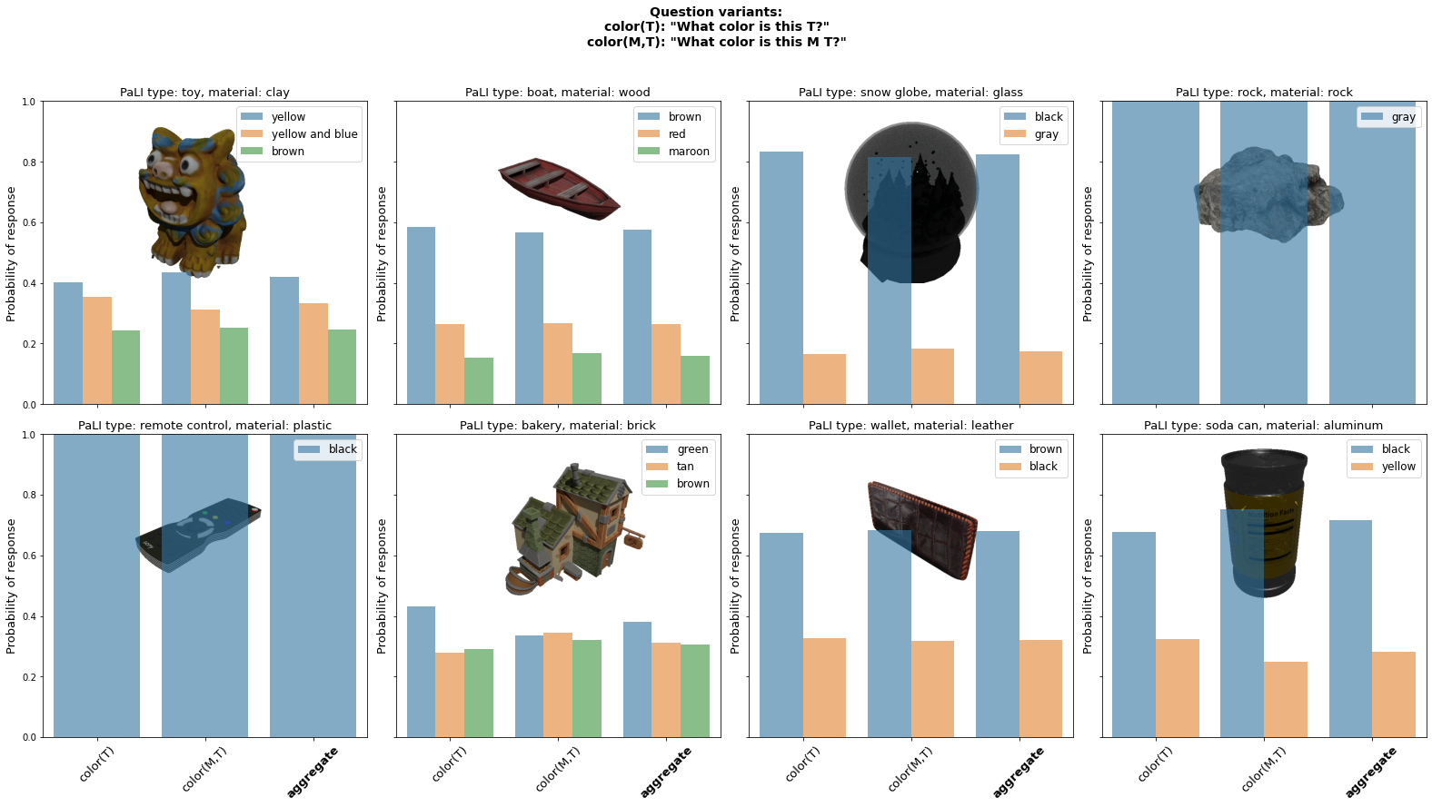
Figure 18: Variations of questions per property for a fixed set of objects (contd).

 

 

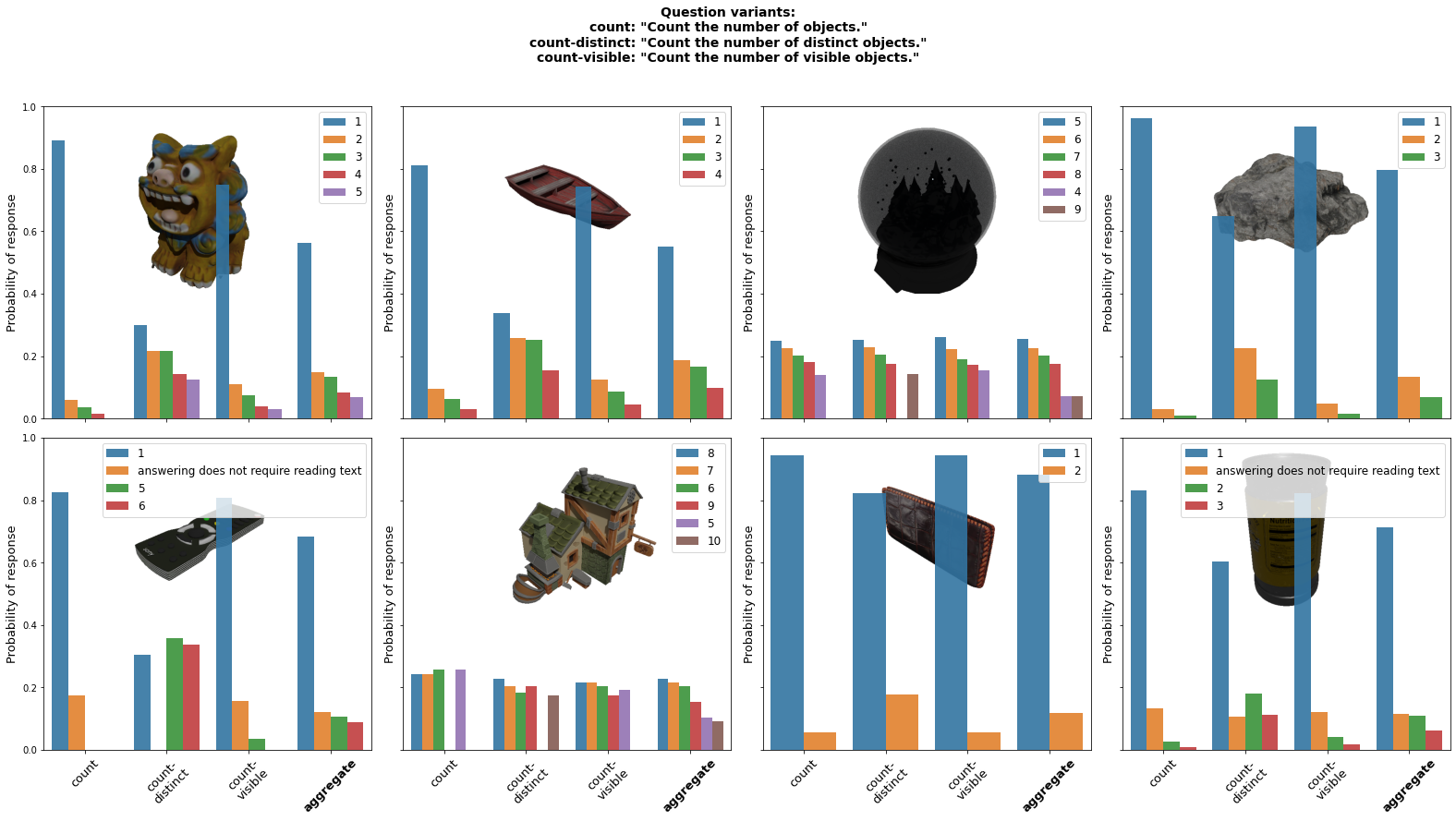
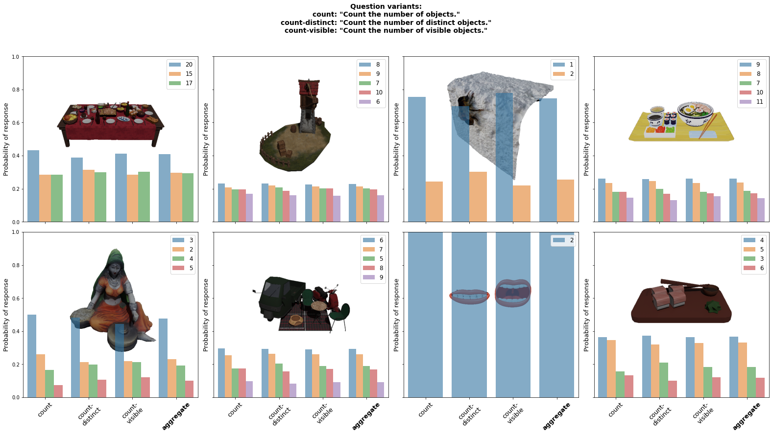
Figure 19: Variations of questions to infer object count. We show the prior set of objects (above), then a set of multi-object scenes (below).

References

- Alayrac et al. [2022] Jean-Baptiste Alayrac, Jeff Donahue, Pauline Luc, Antoine Miech, Iain Barr, Yana Hasson, Karel Lenc, Arthur Mensch, Katherine Millican, Malcolm Reynolds, et al. Flamingo: a visual language model for few-shot learning. NeurIPS, 35:23716–23736, 2022.
- Cer et al. [2018] Daniel Cer, Yinfei Yang, Sheng-yi Kong, Nan Hua, Nicole Limtiaco, Rhomni St John, Noah Constant, Mario Guajardo-Cespedes, Steve Yuan, Chris Tar, et al. Universal sentence encoder. arXiv preprint arXiv:1803.11175, 2018.
- Chen et al. [2023a] Xi Chen, Josip Djolonga, Piotr Padlewski, Basil Mustafa, Soravit Changpinyo, Jialin Wu, Carlos Riquelme Ruiz, Sebastian Goodman, Xiao Wang, Yi Tay, et al. Pali-x: On scaling up a multilingual vision and language model. arXiv preprint arXiv:2305.18565, 2023a.
- Chen et al. [2023b] Xi Chen, Xiao Wang, Soravit Changpinyo, AJ Piergiovanni, Piotr Padlewski, Daniel Salz, Sebastian Goodman, Adam Grycner, Basil Mustafa, Lucas Beyer, Alexander Kolesnikov, Joan Puigcerver, Nan Ding, Keran Rong, Hassan Akbari, Gaurav Mishra, Linting Xue, Ashish V Thapliyal, James Bradbury, Weicheng Kuo, Mojtaba Seyedhosseini, Chao Jia, Burcu Karagol Ayan, Carlos Riquelme Ruiz, Andreas Peter Steiner, Anelia Angelova, Xiaohua Zhai, Neil Houlsby, and Radu Soricut. PaLI: A jointly-scaled multilingual language-image model. In ICLR, 2023b.
- Chung et al. [2022] Hyung Won Chung, Le Hou, Shayne Longpre, Barret Zoph, Yi Tay, William Fedus, Yunxuan Li, Xuezhi Wang, Mostafa Dehghani, Siddhartha Brahma, et al. Scaling instruction-finetuned language models. arXiv preprint arXiv:2210.11416, 2022.
- Collins et al. [2022] Jasmine Collins, Shubham Goel, Kenan Deng, Achleshwar Luthra, Leon Xu, Erhan Gundogdu, Xi Zhang, Tomas F Yago Vicente, Thomas Dideriksen, Himanshu Arora, Matthieu Guillaumin, and Jitendra Malik. Abo: Dataset and benchmarks for real-world 3d object understanding. CVPR, 2022.
- Community [2018] Blender Online Community. Blender - a 3D modelling and rendering package. Blender Foundation, Stichting Blender Foundation, Amsterdam, 2018.
- De Luigi et al. [2023] Luca De Luigi, Damiano Bolognini, Federico Domeniconi, Daniele De Gregorio, Matteo Poggi, and Luigi Di Stefano. Scannerf: a scalable benchmark for neural radiance fields. In Winter Conference on Applications of Computer Vision, 2023. WACV.
- Dehghani et al. [2023] Mostafa Dehghani, Josip Djolonga, Basil Mustafa, Piotr Padlewski, Jonathan Heek, Justin Gilmer, Andreas Peter Steiner, Mathilde Caron, Robert Geirhos, Ibrahim Alabdulmohsin, et al. Scaling vision transformers to 22 billion parameters. In International Conference on Machine Learning, pages 7480–7512. PMLR, 2023.
- Deitke et al. [2023] Matt Deitke, Dustin Schwenk, Jordi Salvador, Luca Weihs, Oscar Michel, Eli VanderBilt, Ludwig Schmidt, Kiana Ehsani, Aniruddha Kembhavi, and Ali Farhadi. Objaverse: A universe of annotated 3d objects. In CVPR, pages 13142–13153, 2023.
- Fang et al. [2023] Yuxin Fang, Wen Wang, Binhui Xie, Quan Sun, Ledell Wu, Xinggang Wang, Tiejun Huang, Xinlong Wang, and Yue Cao. Eva: Exploring the limits of masked visual representation learning at scale. In CVPR, pages 19358–19369, 2023.
- Frostig et al. [2018] Roy Frostig, Matthew James Johnson, and Chris Leary. Compiling machine learning programs via high-level tracing. Systems for Machine Learning, 4(9), 2018.
- Gao et al. [2023] Jensen Gao, Bidipta Sarkar, Fei Xia, Ted Xiao, Jiajun Wu, Brian Ichter, Anirudha Majumdar, and Dorsa Sadigh. Physically grounded vision-language models for robotic manipulation. arXiv preprint arXiv:2309.02561, 2023.
- Gershman and Goodman [2014] Samuel Gershman and Noah Goodman. Amortized inference in probabilistic reasoning. In Proceedings of the annual meeting of the cognitive science society, 2014.
- Gu et al. [2023] Qiao Gu, Alihusein Kuwajerwala, Sacha Morin, Krishna Murthy Jatavallabhula, Bipasha Sen, Aditya Agarwal, Corban Rivera, William Paul, Kirsty Ellis, Rama Chellappa, Chuang Gan, Celso Miguel de Melo, Joshua B. Tenenbaum, Antonio Torralba, Florian Shkurti, and Liam Paull. Conceptgraphs: Open-vocabulary 3d scene graphs for perception and planning, 2023.
- Gupta et al. [2019] Agrim Gupta, Piotr Dollar, and Ross Girshick. Lvis: A dataset for large vocabulary instance segmentation. In CVPR, pages 5356–5364, 2019.
- Gupta and Kembhavi [2023] Tanmay Gupta and Aniruddha Kembhavi. Visual programming: Compositional visual reasoning without training. In CVPR, pages 14953–14962, 2023.
- Ha and Song [2022] Huy Ha and Shuran Song. Semantic abstraction: Open-world 3d scene understanding from 2d vision-language models. In 6th Annual Conference on Robot Learning, 2022.
- Han et al. [2020] Zhizhong Han, Chao Chen, Yu-Shen Liu, and Matthias Zwicker. Shapecaptioner: Generative caption network for 3d shapes by learning a mapping from parts detected in multiple views to sentences. In Proceedings of the 28th ACM International Conference on Multimedia, pages 1018–1027, 2020.
- Hermann et al. [2020] Katherine Hermann, Ting Chen, and Simon Kornblith. The origins and prevalence of texture bias in convolutional neural networks. In NeurIPS, pages 19000–19015. Curran Associates, Inc., 2020.
- Hong et al. [2023] Yining Hong, Haoyu Zhen, Peihao Chen, Shuhong Zheng, Yilun Du, Zhenfang Chen, and Chuang Gan. 3d-llm: Injecting the 3d world into large language models. arXiv preprint arXiv:2307.12981, 2023.
- Jia et al. [2021] Chao Jia, Yinfei Yang, Ye Xia, Yi-Ting Chen, Zarana Parekh, Hieu Pham, Quoc Le, Yun-Hsuan Sung, Zhen Li, and Tom Duerig. Scaling up visual and vision-language representation learning with noisy text supervision. In International conference on machine learning, pages 4904–4916. PMLR, 2021.
- Kojima et al. [2022] Takeshi Kojima, Shixiang Shane Gu, Machel Reid, Yutaka Matsuo, and Yusuke Iwasawa. Large language models are zero-shot reasoners. NeurIPS, 35:22199–22213, 2022.
- Koo et al. [2022] Juil Koo, Ian Huang, Panos Achlioptas, Leonidas J Guibas, and Minhyuk Sung. Partglot: Learning shape part segmentation from language reference games. In Proceedings of the IEEE/CVF Conference on Computer Vision and Pattern Recognition, pages 16505–16514, 2022.
- Kudo and Richardson [2018] Taku Kudo and John Richardson. Sentencepiece: A simple and language independent subword tokenizer and detokenizer for neural text processing. arXiv preprint arXiv:1808.06226, 2018.
- Kuznetsova et al. [2020] Alina Kuznetsova, Hassan Rom, Neil Alldrin, Jasper Uijlings, Ivan Krasin, Jordi Pont-Tuset, Shahab Kamali, Stefan Popov, Matteo Malloci, Alexander Kolesnikov, et al. The open images dataset v4: Unified image classification, object detection, and visual relationship detection at scale. IJCV, 128(7):1956–1981, 2020.
- Li et al. [2022a] Dongxu Li, Junnan Li, Hung Le, Guangsen Wang, Silvio Savarese, and Steven CH Hoi. Lavis: A library for language-vision intelligence. arXiv preprint arXiv:2209.09019, 2022a.
- Li et al. [2022b] Junnan Li, Dongxu Li, Caiming Xiong, and Steven Hoi. Blip: Bootstrapping language-image pre-training for unified vision-language understanding and generation. In International Conference on Machine Learning, pages 12888–12900. PMLR, 2022b.
- Li et al. [2023] Junnan Li, Dongxu Li, Silvio Savarese, and Steven Hoi. Blip-2: Bootstrapping language-image pre-training with frozen image encoders and large language models. arXiv preprint arXiv:2301.12597, 2023.
- Li et al. [2019] Liunian Harold Li, Mark Yatskar, Da Yin, Cho-Jui Hsieh, and Kai-Wei Chang. Visualbert: A simple and performant baseline for vision and language. arXiv preprint arXiv:1908.03557, 2019.
- Luo et al. [2023] Tiange Luo, Chris Rockwell, Honglak Lee, and Justin Johnson. Scalable 3d captioning with pretrained models. NeurIPS, 36, 2023.
- Marino et al. [2018] Joe Marino, Yisong Yue, and Stephan Mandt. Iterative amortized inference. In International Conference on Machine Learning, pages 3403–3412. PMLR, 2018.
- Miller [1995] George A Miller. Wordnet: a lexical database for english. Communications of the ACM, 38(11):39–41, 1995.
- Naseer et al. [2021] Muhammad Muzammal Naseer, Kanchana Ranasinghe, Salman H Khan, Munawar Hayat, Fahad Shahbaz Khan, and Ming-Hsuan Yang. Intriguing properties of vision transformers. In NeurIPS, pages 23296–23308. Curran Associates, Inc., 2021.
- O’Connell et al. [2023] Thomas P O’Connell, Tyler Bonnen, Yoni Friedman, Ayush Tewari, Josh B Tenenbaum, Vincent Sitzmann, and Nancy Kanwisher. Approaching human 3d shape perception with neurally mappable models. arXiv preprint arXiv:2308.11300, 2023.
- OpenAI [2023] OpenAI. Gpt-4 technical report, 2023.
- Piergiovanni et al. [2022] AJ Piergiovanni, Weicheng Kuo, and Anelia Angelova. Pre-training image-language transformers for open-vocabulary tasks. arXiv preprint arXiv:2209.04372, 2022.
- Radford et al. [2021] Alec Radford, Jong Wook Kim, Chris Hallacy, Aditya Ramesh, Gabriel Goh, Sandhini Agarwal, Girish Sastry, Amanda Askell, Pamela Mishkin, Jack Clark, et al. Learning transferable visual models from natural language supervision. In International conference on machine learning, pages 8748–8763. PMLR, 2021.
- Raffel et al. [2020] Colin Raffel, Noam Shazeer, Adam Roberts, Katherine Lee, Sharan Narang, Michael Matena, Yanqi Zhou, Wei Li, and Peter J Liu. Exploring the limits of transfer learning with a unified text-to-text transformer. The Journal of Machine Learning Research, 21(1):5485–5551, 2020.
- Roberts et al. [2022] Adam Roberts, Hyung Won Chung, Anselm Levskaya, Gaurav Mishra, James Bradbury, Daniel Andor, Sharan Narang, Brian Lester, Colin Gaffney, Afroz Mohiuddin, Curtis Hawthorne, Aitor Lewkowycz, Alex Salcianu, Marc van Zee, Jacob Austin, Sebastian Goodman, Livio Baldini Soares, Haitang Hu, Sasha Tsvyashchenko, Aakanksha Chowdhery, Jasmijn Bastings, Jannis Bulian, Xavier Garcia, Jianmo Ni, Andrew Chen, Kathleen Kenealy, Jonathan H. Clark, Stephan Lee, Dan Garrette, James Lee-Thorp, Colin Raffel, Noam Shazeer, Marvin Ritter, Maarten Bosma, Alexandre Passos, Jeremy Maitin-Shepard, Noah Fiedel, Mark Omernick, Brennan Saeta, Ryan Sepassi, Alexander Spiridonov, Joshua Newlan, and Andrea Gesmundo. Scaling up models and data with t5x and seqio. arXiv preprint arXiv:2203.17189, 2022.
- Sun et al. [2017] Chen Sun, Abhinav Shrivastava, Saurabh Singh, and Abhinav Gupta. Revisiting unreasonable effectiveness of data in deep learning era. In ICCV, pages 843–852, 2017.
- Surís et al. [2023] Dídac Surís, Sachit Menon, and Carl Vondrick. Vipergpt: Visual inference via python execution for reasoning. arXiv preprint arXiv:2303.08128, 2023.
- Tay et al. [2022] Yi Tay, Mostafa Dehghani, Vinh Q Tran, Xavier Garcia, Dara Bahri, Tal Schuster, Huaixiu Steven Zheng, Neil Houlsby, and Donald Metzler. Unifying language learning paradigms. arXiv preprint arXiv:2205.05131, 2022.
- Vaswani et al. [2017] Ashish Vaswani, Noam Shazeer, Niki Parmar, Jakob Uszkoreit, Llion Jones, Aidan N Gomez, Łukasz Kaiser, and Illia Polosukhin. Attention is all you need. NeurIPS, 30, 2017.
- Wu et al. [2023] Tong Wu, Jiarui Zhang, Xiao Fu, Yuxin Wang, Jiawei Ren, Liang Pan, Wayne Wu, Lei Yang, Jiaqi Wang, Chen Qian, et al. Omniobject3d: Large-vocabulary 3d object dataset for realistic perception, reconstruction and generation. In CVPR, pages 803–814, 2023.
- Wu et al. [2016] Yonghui Wu, Mike Schuster, Zhifeng Chen, Quoc V Le, Mohammad Norouzi, Wolfgang Macherey, Maxim Krikun, Yuan Cao, Qin Gao, Klaus Macherey, et al. Google’s neural machine translation system: Bridging the gap between human and machine translation. arXiv preprint arXiv:1609.08144, 2016.
- Zareian et al. [2021] Alireza Zareian, Kevin Dela Rosa, Derek Hao Hu, and Shih-Fu Chang. Open-vocabulary object detection using captions. In Proceedings of the IEEE/CVF Conference on Computer Vision and Pattern Recognition, pages 14393–14402, 2021.
- Zhai et al. [2022] Xiaohua Zhai, Alexander Kolesnikov, Neil Houlsby, and Lucas Beyer. Scaling vision transformers. In CVPR, pages 12104–12113, 2022.
- Zhu et al. [2023] Deyao Zhu, Jun Chen, Kilichbek Haydarov, Xiaoqian Shen, Wenxuan Zhang, and Mohamed Elhoseiny. Chatgpt asks, blip-2 answers: Automatic questioning towards enriched visual descriptions. arXiv preprint arXiv:2303.06594, 2023.