Error estimation of different schemes to measure spin-squeezing inequalities

Abstract

How can we analyze quantum correlations in large and noisy systems without quantum state tomography? An established method is to measure total angular momenta and employ the so-called spin-squeezing inequalities based on their expectations and variances. This allows to detect metrologically useful entanglement, but efficient strategies for estimating such non-linear quantities have yet to be determined. In this paper, we focus on the measurement of spin-squeezing inequalities in multi-qubit systems. We show that spin-squeezing inequalities can not only be evaluated by measurements of the total angular momentum but also by two-qubit correlations, either involving all pair correlations or randomly chosen pair correlations. Then we analyze the estimation errors of our approaches in terms of a hypothesis test. For this purpose, we discuss how error bounds can be derived for non-linear estimators with the help of their variances, characterizing the probability of falsely detecting a separable state as entangled. Our methods can be applied for the statistical treatment of other non-linear parameters of quantum states.

I Introduction

Spin-squeezing was first introduced in the context of metrology. It was recognized that the precision of a measurement can be increased with the help of spin-squeezed states [1, 2, 3, 4, 5, 6]. The conditions for spin-squeezing are commonly expressed in terms of the first and second moments of the angular momentum operator. In direction $\alpha=x,y,z$, the angular momentum operator of an $N$-qubit system is given by

$$J_{\alpha}=\frac{1}{2}\sum_{i=1}^{N}\sigma_{\alpha}^{(i)},$$ (1)

where $\sigma_{\alpha}^{(i)}$ is the corresponding Pauli matrix for qubit $i$. In a simplified view, the variance in a direction orthogonal to the mean spin direction is reduced for a spin-squeezed state. This is reflected for instance by the spin-squeezing parameter $\xi_{\text{R}}$ in Ref. [2]. A state that fulfills

$$\xi_{\text{R}}^{2}=\frac{N(\Delta J_{\vec{n}_{\perp}})^{2}}{|\langle{\vec{J}}\rangle|^{2}}<1$$ (2)

is called spin-squeezed. In the above equation, $\langle{\vec{J}}\rangle=(\langle{J_{x}}\rangle,\langle{J_{y}}\rangle,\langle{J_{z}}\rangle)$ is the mean spin direction, i.e., the expectation value of the angular momentum vector. $(\Delta J_{\vec{n}_{\perp}})^{2}$ denotes the smallest variance of the spin in a direction $\vec{n}_{\perp}$ orthogonal to the mean spin direction. This definition is similar to squeezed states of light, where the state also exhibits a reduced variance in a direction in phase space [7]. In Ref. [2], these states are used to improve the sensitivity in Ramsey spectroscopy. Experimentally, spin-squeezed states have been successfully prepared in atomic ensembles and especially in Bose-Einstein condensates [8, 9, 10, 11, 12, 13, 14, 15].

The advantage of spin-squeezed states in metrology is due to quantum-mechanical correlations between the particles [1]. A connection to entanglement was first shown in Ref. [16]. All states that are not entangled fulfill the inequality

$$\frac{N(\Delta J_{z})^{2}}{\expectationvalue{J_{x}}^{2}+\expectationvalue{J_{y}}^{2}}\geq 1.$$ (3)

Thus, a violation implies that the state is entangled. After the formulation of the first spin-squeezing inequality, many other criteria have been found [17, 18, 19, 20, 21]. Moreover, these criteria have been readily applied in experiments [16, 22, 23, 24, 25]. For example, the original spin-squeezing inequality is introduced in Ref. [16] to verify entanglement in a Bose-Einstein condensate.

In this paper, we consider the problem of estimating spin-squeezing parameters from experimental data. For this purpose, we discuss the optimal spin-squeezing inequalities of Refs. [20, 21]. As a first approach, we consider an estimator based on the well-known sample mean and sample variance. This serves as a benchmark for the second and third approaches, which are formulated in terms of pair correlations. The second approach relies on the measurement of all pair correlations and single qubits. This in turn can be randomized. Instead of looking at all pair correlations and single qubits, the qubit pairs and single qubits are measured randomly. The approach to measure the qubits at random follows the methods in Refs. [26, 27, 28]. In Ref. [26], the fidelity of an $N$-qubit system is estimated. For this purpose, the Pauli measurements are performed at random according to some probability distribution that is determined by the target state. The authors show that this approach requires less resources than full tomography. Moreover, measurements from a set of two-outcome observables are drawn randomly in Ref. [27, 28] to verify entanglement.

The investigation of different schemes to test spin-squeezing inequalities is experimentally motivated. For different experimental set-ups some of the approaches are more suitable then others. For example, in Bose-Einstein condensates the total angular momenta can usually be resolved by absorption images [11, 29, 24]. As no measurements on single atoms can be performed, an estimator that relies on the total angular momentum is appropriate. In contrast, ion traps usually allow the read-out of the individual atoms. However, the simultaneous read-out of the ions by fluorescence measurements becomes challenging with increasing number of ions in the trap [30]. In this case, the schemes that rely on pair correlations provide an alternative. Moreover, the schemes enable to evaluate spin-squeezing parameters from spin-spin correlations that have already been obtained in experiments [31].

Finally, spin-squeezing parameters are usually formulated in terms of the first and second moments of angular momentum operators and thus constitute non-linear quantities in the quantum state. To compare the different approaches, we discuss a statistical analysis that can be applied to non-linear estimators. Consequently, our methods will be useful to estimate other nonlinear parameters (e.g., the purity or the Fisher information) as well.

We start in Sec. II.1 by introducing the optimal spin-squeezing inequalities. These inequalities are used to demonstrate the three approaches. The value of the spin-squeezing inequalities can only be estimated from experimental data. Hence, we formulate the problem as a hypothesis test in Sec. II.2. Thereafter, we will explain the three approaches to estimate the spin-squeezing parameters in detail in Sec. III. Finally, we show how the statistics of the derived non-linear estimators can be analyzed in Sec. IV.

II Preliminaries

II.1 Optimal spin-squeezing inequalities

After the discovery of the original spin-squeezing inequality given by Eq. (3), refined spin-squeezing inequalities have been found. Here, we will focus on the optimal spin-squeezing inequalities formulated in Refs. [20, 21]. The aim of these inequalities is to detect entanglement and thus they differ from the spin-squeezing inequalities used in metrology. Though, they are of the same form and use both the first and second moments of the angular momentum operators given in Eq. (1). On the level of pure states, a quantum state of $N$ qubits is defined as fully separable if it can be written as a product state, i.e.,

$$\ket{\psi}=\ket{\psi_{1}}\otimes\ket{\psi_{2}}\otimes\ldots\otimes\ket{\psi_{N}},$$ (4)

where $\ket{\psi_{i}}$ is the state of qubit $i$. Accordingly, a state is entangled if it cannot be written as a product state [32]. This notion can be extended to mixed states. A mixed state is called fully separable in case it can be written as a convex combination of product states, i.e.,

$$\rho=\sum_{k}p_{k}\rho_{k}^{(1)}\otimes\ldots\otimes\rho_{k}^{(N)},$$ (5)

where $p_{k}$ is a probability with $\sum_{k}p_{k}=1$.

Since spin-squeezing inequalities only use limited information in terms of the first and second moments of the total angular momenta, the characterisation of entanglement is not complete. In this paper, we focus on the optimal spin-squeezing inequalities [20, 21] that detect the maximal amount of entangled states:

$$\expectationvalue{J_{x}^{2}}+\expectationvalue{J_{y}^{2}}+\expectationvalue{J_{z}^{2}} \leq\frac{N(N+2)}{4},$$ (6a)

$$(\Delta J_{x})^{2}+(\Delta J_{y})^{2}+(\Delta J_{z})^{2} \geq\frac{N}{2},$$ (6b)

$$\expectationvalue{J_{k}^{2}}+\expectationvalue{J_{l}^{2}}-\frac{N}{2} \leq(N-1)(\Delta J_{m})^{2},$$ (6c)

$$(N-1)\left[(\Delta J_{k})^{2}+(\Delta J_{l})^{2}\right] \geq\expectationvalue{J_{m}^{2}}+\frac{N(N-2)}{4}.$$ (6d)

The above inequalities are fulfilled by all separable states. In Eq. (6), $(k,l,m)$ is a permutation of $(x,y,z)$. Whereas Eq.(6a) is valid for all quantum states, a violation of Eq.(6b)-(6d) implies entanglement. For fixed mean spin $(\langle{J_{x}}\rangle,\langle{J_{y}}\rangle,\langle{J_{z}}\rangle)$, the inequalities in Eq. (6) define a polytope in the space of $(\langle{J_{x}^{2}}\rangle,\langle{J_{y}^{2}}\rangle,\langle{J_{z}^{2}}\rangle)$ [21]. In the limit $N\rightarrow\infty$ but also for special cases of finite $N$, there exists a separable state for all points inside the polytope. In these cases, the inequalities identify the maximal amount of entangled states that can be detected by the first and second moments of the angular momentum operators.

For example, Eq. (6b) detects many-body singlet states as entangled [21]. These states are characterized by

$$\begin{split}(\langle{J_{x}}\rangle,\langle{J_{y}}\rangle,\langle{J_{z}}\rangle)&=(0,0,0),\\ (\langle{J_{x}^{2}}\rangle,\langle{J_{y}^{2}}\rangle,\langle{J_{z}^{2}}\rangle)&=(0,0,0).\end{split}$$ (7)

As the left-hand side of Eq. (6b) is non-negative, we see that Eq. (6b) is maximally violated by the many-body singlet states. To visualize the state, we can make use of the collective Bloch sphere [33]. In this representation, the mean spin of the states is plotted. In addition, the variances $(\Delta J_{x})^{2},(\Delta J_{y})^{2},(\Delta J_{z})^{2}$ are used to give the uncertainty. For many-body singlet states, both the mean spin and the variances are zero. Hence, many-body singlet states correspond to the red dot at the origin in Fig. 1. A specific example of a many-body singlet state for an even number of qubits $N$ is given by

$$\ket{\Psi^{-}}=\bigotimes_{k=1}^{N/2}\ket{\psi^{-}},$$ (8)

with the two-qubit singlet state $\ket{\psi^{-}}=\frac{1}{\sqrt{2}}(\ket{01}-\ket{10})$. We show in App. C.1 that $\ket{\Psi^{-}}$ indeed fulfills the defining property in Eq. (7).

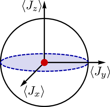
Figure 1: Visualization of the singlet state $\ket{\Psi^{-}}$ (red) and the Dicke state $\ket{D_{N,N/2}}$ (blue) on the collective Bloch sphere [33]. Singlet states are characterized by vanishing mean spin $\langle{\vec{J}}\rangle=0$ and variances. Hence, the singlet state $\ket{\Psi^{-}}$ corresponds to the red dot at the origin. The Dicke state $\ket{D_{N,N/2}}$ is also at the origin, though it has a nonzero variance in the $x$-$y$-plane that is shown by the blue shaded area.

The inequality in Eq. (6c) is in turn maximally violated by the symmetric Dicke state $\ket{D_{N,N/2}}$ with $m=\frac{N}{2}$ excitations [21]. For $m$ excitations, the symmetric Dicke state is defined as

$$\ket{D_{N,m}}=\binom{N}{m}^{-\frac{1}{2}}\sum_{k}P_{k}(\ket{1_{1},\ldots,1_{m},0_{m+1},\ldots,0_{N}}),$$ (9)

where the sum iterates over all distinct permutations $P_{k}$ of the qubits and $\binom{N}{m}$ denotes the binomial coefficient. The first and second moments of the angular momenta of the Dicke states are

$$\begin{split}(\langle{J_{x}}\rangle,\langle{J_{y}}\rangle,\langle{J_{z}}\rangle)&=\left(0,0,\frac{N}{2}-m\right),\\ (\langle{J_{x}^{2}}\rangle,\langle{J_{y}^{2}}\rangle,\langle{J_{z}^{2}}\rangle)&=\left(f_{N,m},f_{N,m},[\frac{N}{2}-m]^{2}\right),\end{split}$$ (10)

where $f_{N,m}=\frac{N}{4}+\frac{m(N-m)}{2}$. Hence, the Dicke state $|D_{N,N/2}\rangle$ with $m=\frac{N}{2}$ excitations is also located at the origin of the collective Bloch sphere. However, the variances $(\Delta J_{x})^{2}$ and $(\Delta J_{y})^{2}$ are non-zero. They are of the order $\mathcal{O}(N^{2})$, which is of the same magnitude as the radius of the Bloch sphere. This is shown as the blue circle in Fig. 1.

Finally, many-body singlet states violate also the fourth spin-squeezing inequality in Eq. (6d) [21].

To evaluate the spin-squeezing inequalities from experimental data, we define corresponding parameters that include the quantities to estimate:

$$\xi_{a} =\expectationvalue{J_{x}^{2}}+\expectationvalue{J_{y}^{2}}+\expectationvalue{J_{z}^{2}},$$ (11a)

$$\xi_{b} =(\Delta J_{x})^{2}+(\Delta J_{y})^{2}+(\Delta J_{z})^{2},$$ (11b)

$$\xi_{c} =\expectationvalue{J_{k}^{2}}+\expectationvalue{J_{l}^{2}}-(N-1)(\Delta J_{m})^{2},$$ (11c)

$$\xi_{d} =(N-1)\left[(\Delta J_{k})^{2}+(\Delta J_{l})^{2}\right]-\expectationvalue{J_{m}^{2}}.$$ (11d)

Then, the inequalities in (6) imply for separable states: $\xi_{a}\leq\frac{N(N+2)}{4}$, $\xi_{b}\geq\frac{N}{2}$, $\xi_{c}\leq\frac{N}{2}$ and $\xi_{d}\geq\frac{N(N-2)}{4}$.

II.2 Hypothesis tests

Although the spin-squeezing parameters, $\xi=\xi_{u}$ for $u=a,b,c,d$ in Eq. (11), contain terms that can be directly measured in an experiment, their exact values cannot be obtained from a finite number of measurement repetitions. In the following, we consider how to estimate the spin-squeezing parameters in practice.

Let us begin by defining an estimator $\tilde{\xi}$ for $\xi$ (which we denote by a tilde). An estimator $\tilde{\xi}$ is a random variable according to some probability distribution, which can be created from experimental data. It is common to require that the estimator is unbiased, meaning that the expectation coincides with the target parameter value, i.e.,

$$\mathbb{E}[\tilde{\xi}]=\xi.$$ (12)

But due to the finite statistics, the estimator $\tilde{\xi}$ exhibits fluctuations, and there are unavoidable errors in the estimation. The presence of such errors yields a finite probability for a violation of a spin-squeezing inequality even though the actual quantum state is separable. For this reason, we formulate the question of whether a state is entangled as a hypothesis test. We apply statistical methods described in Ref. [34], where the methods are used in the context of quantum state verification and fidelity estimation.

To set up the statistical test, we first formulate the hypotheses:

• Null hypothesis $\mathbf{H_{0}}$: The quantum state is fully separable, i.e. $\rho=\sum_{k}p_{k}\rho_{k}^{(1)}\otimes\ldots\otimes\rho_{k}^{(N)}$.

• Alternative hypothesis $\mathbf{H_{1}}$: The quantum state is not fully separable, i.e., it is entangled.

Based on a decision rule, the null hypothesis $H_{0}$ is either accepted or rejected. For example, the decision rule is of the form: If $\tilde{\xi}\leq\varepsilon_{c}$ for some threshold $\varepsilon_{c}$ we accept $H_{0}$, whereas in case $\tilde{\xi}>\varepsilon_{c}$ we reject it. Note that $\varepsilon_{c}$ does not necessarily correspond to the upper bound of the spin-squeezing parameter for separable states. There are two possible types of errors. Type I error denotes the case that $H_{0}$ is rejected even though $H_{0}$ is true. The opposite case that $H_{0}$ is accepted when in fact $H_{1}$ is true is called Type II error.

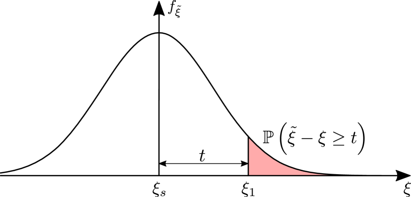
Figure 2: Upper bound of the $p$-value. The plot shows an exemplary probability density function $f_{\tilde{\xi}}$ of the estimator for a separable state with spin-squeezing parameter $\xi=\xi_{s}$. $\xi_{s}$ denotes the extremal value that can be achieved by separable states. To observe an outcome $\xi_{1}$, the estimator has to deviate at least by $t=\xi_{1}-\xi_{s}$ from its mean. The probability $\mathbb{P}(\tilde{\xi}-\xi\geq t)$ for this to happen corresponds to the red area.

We are interested in the significance level $\alpha$ of an experimental result. This means that the probability to detect a state as entangled even though it was separable, i.e., the probability for Type I error, is at most $\alpha$:

$$\mathbb{P}(\tilde{\xi}>\varepsilon_{c}|H_{0})\leq\alpha.$$ (13)

However, it is difficult to fix a threshold $\varepsilon_{c}$, as the probability distribution of the estimator depends on the quantum state and is unknown. Rather, we use the $p$-value to assess the significance of an experimental outcome $\xi_{1}$. The $p$-value denotes the probability that an outcome at least as extreme as $\xi_{1}$ is observed under the assumption that $H_{0}$ is true:

$$p=\mathbb{P}\left(\tilde{\xi}\geq\xi_{1}\Big{|}H_{0}\right).$$ (14)

The $p$-value depends on the specific separable state at hand. We can derive an upper bound of the $p$-value by considering a state that saturates the separable bound, i.e., $\xi=\xi_{s}$. This is shown in Fig. 2. For a separable state the estimator has to deviate at least by $t=\xi_{1}-\xi_{s}\geq 0$ from its mean, in case a violation is observed. As a result, we obtain the inequality

$$p\leq\mathbb{P}\left(\tilde{\xi}-\xi\geq t\right).$$ (15)

The probability on the right hand side can in turn be bounded with the help of concentration inequalities, e.g., Cantelli’s inequality [35]. These are large deviation bounds that typically involve the number of repetitions and thus connect the $p$-value to the number of experimental runs. Finally, we say that a result with a certain $p$-value has a confidence level of $\gamma=1-p$. As a result, we can determine the necessary number of repetitions to assure a given confidence level.

III Three ways to measure spin-squeezing inequalities

In this section, we are going to present the three measurement schemes to obtain the spin-squeezing parameters. As the expectation value is linear, we give the unbiased estimators for the terms in the spin-squeezing parameters separately. We start with the scheme that uses total spin measurements. For this scheme we discuss the estimators for the expectation value $\langle{J_{\alpha}^{2}}\rangle$ and the variance $(\Delta J_{\alpha})^{2}$. In contrast, for the approaches that are based on pair correlations we explain the estimators for $\langle{J_{\alpha}^{2}}\rangle$ and $(\Delta J_{\alpha})^{2}$, but also for $\langle{J_{\alpha}}\rangle$.

III.1 Estimator based on the total spin

The first approach relies on the measurement of the total spin. To evaluate the spin-squeezing parameters, the observables $J_{x},J_{y}$ and $J_{z}$ , that are defined in Eq. (1), are measured, i.e., the total spin in $x$-, $y$- and $z$-direction. In each direction $\alpha\in\{x,y,z\}$ the measurement is repeated $K_{\text{TS}}$-times. We denote the measurement results of the $k$-th repetition as $m_{\alpha}^{(k)}$. The possible outcomes are $m_{\alpha}^{(k)}\in\{-\frac{N}{2},-\frac{N}{2}+1,\ldots,\frac{N}{2}\}$. This is depicted in Fig. 3.

Figure 3: Measurement scheme for the estimators $\widetilde{\expectationvalue{J_{\alpha}^{2}}}_{\text{TS}}$ and $\widetilde{(\Delta J_{\alpha})^{2}}_{\text{TS}}$. In each repetition $k$, the total spin of the system is measured. In an ion trap, this can be done by resonance fluorescence [36], which gives also access to the spin of the individual qubits. The figure includes an image of trapped ${}^{171}\text{Yb}^{+}$ ions, which is reprinted from [36].

From the experimental data, we can infer the expectation value by the sample mean:

$$\widetilde{\expectationvalue{J_{\alpha}^{2}}}_{\text{TS}}=\sum_{k=1}^{K_{\text{TS}}}\frac{(m_{\alpha}^{(k)})^{2}}{K_{\text{TS}}}.$$ (16)

In the above estimator we used that the result $m_{\alpha}$ for a measurement of $J_{\alpha}$ implies the result $m_{\alpha}^{2}$ for a measurement of $J_{\alpha}^{2}$.

Correspondingly, we can estimate the variance by the sample variance:

$$\widetilde{(\Delta J_{\alpha})^{2}}_{\text{TS}}=\frac{1}{K_{\text{TS}}-1}\sum_{k=1}^{K_{\text{TS}}}\left(m_{\alpha}^{(k)}-\widetilde{\expectationvalue{J_{\alpha}}}_{\text{TS}}\right)^{2},$$ (17)

where $\widetilde{\expectationvalue{J_{\alpha}}}_{\text{TS}}=\sum_{k=1}^{K_{\text{TS}}}\frac{m_{\alpha}^{(k)}}{K_{\text{TS}}}$ denotes the estimator for the expectation value $\expectationvalue{J_{\alpha}}$. Both, the sample mean and the sample variance are unbiased estimators [37], i.e., it is $\mathbb{E}[\widetilde{\expectationvalue{J_{\alpha}^{2}}}_{\text{TS}}]=\langle{J_{\alpha}^{2}}\rangle$ and $\mathbb{E}[\widetilde{(\Delta J_{\alpha})^{2}}_{\text{TS}}]=(\Delta J_{\alpha})^{2}$. With these building blocks, we can write down unbiased estimators for the spin-squeezing parameters in Eq. (11), e.g.,

$$(\tilde{\xi}_{c})_{\text{TS}}=\widetilde{\langle{J_{x}^{2}}\rangle}_{\text{TS}}+\widetilde{\langle{J_{y}^{2}}\rangle}_{\text{TS}}+(N-1)\widetilde{(\Delta J_{z})^{2}}_{\text{TS}}.$$ (18)

We note that the three estimators on the right-hand side of the above equation rely on the outcomes of spin measurements in different directions. The data is thus obtained in different experimental runs and the estimators are statistically independent.

Moreover, the total spin in each direction is measured $K_{\text{TS}}$-times. The estimator in Eq. (18) thus requires in total $3K_{\text{TS}}$ state samples.

III.2 Estimator based on pair correlations

Instead of the total spin, an estimator can also be formulated in terms of pair correlations. This is motivated by the decomposition of the expectation value $\langle{J_{\alpha}^{2}}\rangle$ in two-qubit correlations:

$$\langle{J_{\alpha}^{2}}\rangle=\frac{N}{4}+\frac{1}{4}\sum_{i\neq j}\langle\sigma_{\alpha}^{(i)}\sigma_{\alpha}^{(j)}\rangle.$$ (19)

We can thus estimate the expectation value $\langle{J_{\alpha}^{2}}\rangle$ by measuring the correlations of all distinct qubit pairs (AP). For each pair $P=(P_{1},P_{2})$ with $P_{1}\neq P_{2}$, the two-qubit correlation $\langle{\sigma_{\alpha}^{(P_{1})}\sigma_{\alpha}^{(P_{2})}}\rangle$ is measured $K_{\text{AP}}$-times. The corresponding estimator reads

$$\widetilde{\langle{J_{\alpha}^{2}}\rangle}_{\text{AP}}=\frac{N}{4}+\frac{1}{K_{\text{AP}}}\sum_{P}\sum_{k=1}^{K_{\text{AP}}}s_{\alpha}^{(P_{1},k)}s_{\alpha}^{(P_{2},k)}.$$ (20)

In the above equation, $s_{\alpha}^{(P_{1/2},k)}$ denotes the spin in direction $\alpha$ of qubit $P_{1/2}$ in the $k$-th measurement repetition of the pair $P$. This scheme is visualized in Fig. 4 (a). We show in App. A.1 that the above estimator is unbiased, i.e., $\mathbb{E}[\widetilde{\expectationvalue{J_{\alpha}^{2}}}_{\text{AP}}]=\langle{J_{\alpha}^{2}}\rangle$.

To estimate the variances we propose two different schemes.

Scheme AP1. The first scheme uses the data as presented in Fig. 4 (a), i.e., it estimates the variance with the help of two-qubit correlations. Though, we assume that the measurement results for the individual qubits are captured. The estimator takes the form

$$\begin{split}\widetilde{(\Delta J_{\alpha})^{2}}&{}_{\text{AP}}=\frac{N}{4}+\frac{1}{K_{\text{AP}}}\sum_{P}\sum_{k=1}^{K_{\text{AP}}}s_{\alpha}^{(P_{1},k)}s_{\alpha}^{(P_{2},k)}\\ &-\frac{1}{K_{\text{AP}}(K_{\text{AP}}-1)(N-1)^{2}}\sum_{P,Q}\sum_{k\neq l}^{K_{\text{AP}}}s_{\alpha}^{(P_{1},k)}s_{\alpha}^{(Q_{2},l)}.\end{split}$$ (21)

With the estimators in Eq. (20) and (21) we can compose estimators for the spin-squeezing parameters, e.g.,

$$(\tilde{\xi}_{c})_{\text{AP1}}=\widetilde{\langle{J_{x}^{2}}\rangle}_{\text{AP}}+\widetilde{\langle{J_{y}^{2}}\rangle}_{\text{AP}}+(N-1)\widetilde{(\Delta J_{z})^{2}}_{\text{AP}}.$$ (22)

As $\mathbb{E}[\widetilde{(\Delta J_{\alpha})^{2}}_{\text{AP}}]=(\Delta J_{\alpha})^{2}$ (cf. App. A.1), $(\tilde{\xi}_{c})_{\text{AP1}}$ is also an unbiased estimator of $\xi_{c}$. Again, the three estimators on the right-hand side of Eq. (22) are obtained in different measurements and are thus statistically independent. For each direction all distinct pairs are measured $K_{\text{AP1}}$-times and hence the total number of state samples is $3N(N-1)K_{\text{AP1}}$.

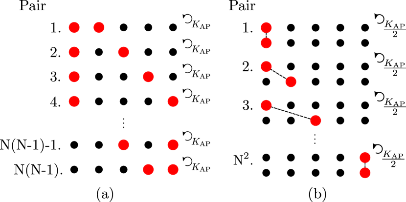
Figure 4: Measurement pattern for (a) $\widetilde{\expectationvalue{J_{\alpha}^{2}}}_{\text{AP}}$ in Eq. (20) as well as $\widetilde{(\Delta J_{\alpha})^{2}}_{\text{AP}}$ in Eq. (21) and (b) $\widetilde{\expectationvalue{J_{\alpha}}^{2}}_{\text{AP}}$ in Eq. (23). In pattern (a) all $N(N-1)$ distinct pairs of qubits are measured $K_{\text{AP}}$-times. In contrast, in pattern (b) all $N^{2}$ pairs are measured, with each qubit observed only in $\frac{K_{\text{AP}}}{2}$ of the experimental runs to ensure statistical independence. The approach AP1 relies only on the measurement pattern (a), whereas for AP2 both the patterns (a) and (b) are used.

Scheme AP2. Alternatively, we can calculate the variance by estimating the expectation value $\expectationvalue{J_{\alpha}}^{2}$ separately, i.e., by $\widetilde{\expectationvalue{J_{\alpha}^{2}}}_{\text{AP}}-\widetilde{\expectationvalue{J_{\alpha}}^{2}}_{\text{AP}}$. For this purpose, we propose to measure the spin of one qubit in each experimental run. From the outcomes, the expectation value $\expectationvalue{J_{\alpha}}^{2}$ can be estimated by multiplying the results of two different experimental runs. This ensures that the two outcomes are statistically independent. To formulate the estimator, we measure all pairs $(i,j)$, where we allow $i=j$. We divide the number of repetitions into two groups. $\frac{K_{\text{AP}}}{2}$ of the times we measure the spin of qubit $i$ and for the remaining repetitions we observe qubit $j$. This results in the following estimator

$$\widetilde{\langle{J_{\alpha}}\rangle^{2}}_{\text{AP}}=\sum_{i,j=1}^{N}\frac{1}{\frac{K_{\text{AP}}}{2}}\sum_{k=1}^{\frac{K_{\text{AP}}}{2}}s_{\alpha}^{(i,2k)}s_{\alpha}^{(j,2k-1)}.$$ (23)

The measurement scheme is depicted in Fig. 4 (b). However, this comes at the expense that the correlations between the two estimators $\widetilde{\expectationvalue{J_{\alpha}^{2}}}_{\text{AP}}$ and $\widetilde{\expectationvalue{J_{\alpha}}^{2}}_{\text{AP}}$ have to be taken into account or two independent data-sets have to be obtained. In the following statistical analysis, we assume that two independent data-sets are used. We show in App. A.1 that Eq. (23) is an unbiased estimator and thus

$$(\tilde{\xi}_{c})_{\text{AP2}}=\widetilde{\langle{J_{x}^{2}}\rangle}_{\text{AP}}+\widetilde{\langle{J_{y}^{2}}\rangle}_{\text{AP}}+(N-1)\left(\widetilde{\langle{J_{z}^{2}}\rangle}_{\text{AP}}-\widetilde{\langle{J_{z}}\rangle^{2}}_{\text{AP}}\right)$$ (24)

obeys $\mathbb{E}[(\tilde{\xi}_{c})_{\text{AP2}}]=\xi_{c}$. In case all estimators on the right-hand side of Eq. (24) are obtained from different data-sets, they are independent. Since the estimator in Eq. (23) uses all pairs of qubits, the total number of state samples is $(4N-3)NK_{\text{AP2}}$.

III.3 Estimator based on random pair correlations

In the previous subsection, we have formulated an estimator that relies on the measurement of all pair correlations and single qubits. Hence, the question arises whether the total number of measurements can be reduced by randomly choosing the pair correlations and qubits that are measured. This can be achieved by introducing additional random variables for the qubit indices $(i,j)$. For $L_{\text{RP}}$ randomly chosen pairs, the estimator for $\langle{J_{\alpha}^{2}}\rangle$ reads

$$\widetilde{\langle{J_{\alpha}^{2}}\rangle}_{\text{RP}}=\frac{N}{4}+\frac{N(N-1)}{K_{\text{RP}}L_{\text{RP}}}\sum_{l=1}^{L_{\text{RP}}}\sum_{k=1}^{K_{\text{RP}}}s_{\alpha}^{(\mathcal{I}_{l},k)}s_{\alpha}^{(\mathcal{J}_{l},k)},$$ (25)

where each pair is measured $K_{\text{RP}}$-times. Similar to Eq. (20), $s_{\alpha}^{(\mathcal{I}_{l},k)}$ and $s_{\alpha}^{(\mathcal{J}_{l},k)}$ denote the spins in the $k$-th measurement of the qubit pair $(\mathcal{I}_{l},\mathcal{J}_{l})$. However, in the above expression the indices $\mathcal{I}_{l}$ and $\mathcal{J}_{l}$ are random variables with $l\in\{1,\ldots,L_{\text{RP}}\}$. As only distinct pairs are of interest, we use the probability distribution

$$\mathbb{P}(\mathcal{I}_{l}=i,\mathcal{J}_{l}=j)=\begin{cases}1/[N(N-1)],&\text{for }i\neq j,\\ 0,&\text{for }i=j.\end{cases}$$ (26)

Also the estimator in Eq. (25) is unbiased, as we show in App. A.2. The scheme is visualized in Fig. 5 (a).

Scheme RP1. From the data that is obtained by the pattern in Fig. 5 (a), we can also estimate the variance $(\Delta J_{\alpha})^{2}$. Let us again denote the outcomes of the spin measurement in direction $\alpha$ for the $k$-th repetition of the $l$-th random pair $(\mathcal{I}_{l},\mathcal{J}_{l})$ by $s_{\alpha}^{(\mathcal{I}_{l},k)}$ and $s_{\alpha}^{(\mathcal{J}_{l},k)}$. Then, an unbiased estimator of $(\Delta J_{\alpha})^{2}$ (cf. App. A.2) is given by

$$\begin{split}\widetilde{(\Delta J_{\alpha})^{2}}_{\text{RP}}&=\frac{N}{4}+\frac{N(N-1)}{L_{\text{RP}}K_{\text{RP}}}\sum_{l=1}^{L_{\text{RP}}}\sum_{k=1}^{K_{\text{RP}}}s_{\alpha}^{(\mathcal{I}_{l},k)}s_{\alpha}^{(\mathcal{J}_{l},k)}\\ &-\frac{N^{2}}{L_{\text{RP}}(L_{\text{RP}}-1)K_{\text{RP}}^{2}}\sum_{l\neq m}^{L_{\text{RP}}}\sum_{k,q=1}^{K_{\text{RP}}}s_{\alpha}^{(\mathcal{I}_{l},k)}s_{\alpha}^{(\mathcal{J}_{m},q)}.\end{split}$$ (27)

The random variables $\mathcal{I}_{l},\mathcal{J}_{l}$ obey the probability distribution in Eq. (26). Finally, we note that $\mathbb{E}[\widetilde{(\Delta J_{\alpha})^{2}}_{\text{RP}}]=(\Delta J_{\alpha})^{2}$ as is shown in App. A.2. With the help of Eq. (25) and Eq. (27) unbiased estimators for the spin-squeezing parameters can be formulated, e.g.,

$$(\tilde{\xi}_{c})_{\text{RP1}}=\widetilde{\langle{J_{x}^{2}}\rangle}_{\text{RP}}+\widetilde{\langle{J_{y}^{2}}\rangle}_{\text{RP}}+(N-1)\widetilde{(\Delta J_{z})^{2}}_{\text{RP}}.$$ (28)

Again, the estimators on the right-hand side of the above equation are statistically independent as they are obtained from different measurements. In total the estimator in Eq. (28) requires $3L_{\text{RP1}}K_{\text{RP1}}$ state samples.

Scheme RP2. Alternatively, we can estimate $\langle{J_{\alpha}}\rangle^{2}$ separately. For this purpose, we choose also $L_{\text{RP}}$ random pairs $(\mathcal{I}_{l},\mathcal{J}_{l})$. However, in each experimental run only one qubit is measured. Thus for $K_{\text{RP}}$ measurements of the pair $(\mathcal{I}_{l},\mathcal{J}_{l})$, we measure $\frac{K_{\text{RP}}}{2}$-times the spin of qubit $\mathcal{I}_{l}$ and $\frac{K_{\text{RP}}}{2}$-times the spin of qubit $\mathcal{J}_{l}$. An estimator is retrieved by the product of the results for each pair $(\mathcal{I}_{l},\mathcal{J}_{l})$, i.e., $\langle{J_{\alpha}}\rangle^{2}$ can be obtained by the estimator

$$\widetilde{\expectationvalue{J_{\alpha}}^{2}}_{\text{RP}}=\frac{2N^{2}}{K_{\text{RP}}L_{\text{RP}}}\sum_{l=1}^{L_{\text{RP}}}\sum_{k=1}^{\frac{K_{\text{RP}}}{2}}s_{\alpha}^{(\mathcal{I}_{l},2k)}s_{\alpha}^{(\mathcal{J}_{l},2k-1)}.$$ (29)

In the derivation of the above estimator all pairs $(i,j)$ have to be considered. Hence, we use the uniform probability distribution $\mathbb{P}(\mathcal{I}_{l}=i,\mathcal{J}_{l}=j)=\frac{1}{N^{2}}$ for all $i,j\in\{1,\ldots,N\}$. Fig. 5 (b) shows a sketch of the estimator. In App. A.2, we proof that the estimator in Eq. (29) is unbiased and hence we can compose for example the unbiased estimator

$$(\tilde{\xi}_{c})_{\text{RP2}}=\widetilde{\langle{J_{x}^{2}}\rangle}_{\text{RP}}+\widetilde{\langle{J_{y}^{2}}\rangle}_{\text{RP}}+(N-1)\bigg{(}\widetilde{\langle{J_{z}^{2}}\rangle}_{\text{RP}}-\widetilde{\expectationvalue{J_{z}}^{2}}_{\text{RP}}\bigg{)}.$$ (30)

The estimators for different spin directions are independent, as they have to be obtained from different data-sets. Finally, we assume that also $\langle{J_{z}^{2}}\rangle$ and $\expectationvalue{J_{z}}^{2}$ are estimated from different data-sets, which assures that all estimators on the right-hand side of Eq. (30) are independent. This approach needs in total $4L_{\text{RP2}}K_{\text{RP2}}$ state samples.

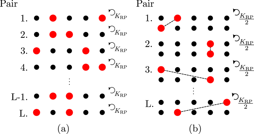
Figure 5: Measurement pattern for (a) $\widetilde{\expectationvalue{J_{\alpha}^{2}}}_{\text{RP}}$ in Eq. (25) and $\widetilde{(\Delta J_{\alpha})^{2}}_{\text{RP}}$ in Eq. (27) and for (b) $\widetilde{\expectationvalue{J_{\alpha}}^{2}}_{\text{RP}}$ in Eq. (29). In pattern (a), $L_{\text{RP}}$ random pair correlations are measured $K_{\text{RP}}$-times each. Pattern (b) in turn uses also $L_{\text{RP}}$ random pairs $(i,j)$, but with the possibility that $i=j$. In $\frac{K_{\text{RP}}}{2}$ of the repetitions qubit $i$ is measured whereas in the other repetitions qubit $j$ is observed. The scheme RP1 is only based on the pattern (a), whereas RP2 relies on both patterns (a) and (b).

IV Statistical analysis

As the estimators are formulated in terms of the random outcomes of the measurements, they are random variables themselves. Hence, they obey a probability distribution. This is exemplary shown for $(\tilde{\xi}_{c})_{\text{TS}}$ in Fig. 6. The following section therefore contains a statistical analysis of the estimators.

We start with the variances to get an insight on the spreading of the probability distribution. This results in state dependent expressions for the variances. Accordingly, we use these results to derive probability bounds with Cantelli’s inequality, which in turn can be used to assess the confidence level or the necessary number of measurements.

IV.1 Variances

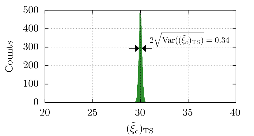
Figure 6: Probability distribution of the estimator $(\tilde{\xi}_{c})_{\text{TS}}$. The simulation has been performed for the 10-qubit Dicke state $|D_{10,5}\rangle$ defined in Eq. (9) with $K_{\text{TS}}=7400$. The histogram contains $99$ bins, but due the the small bin size of $0.02$ they are not well resolved.

In App. B we derive the variances of the estimators. Exemplary, we discuss here the variance of the total-spin estimator $(\tilde{\xi}_{c})_{\text{TS}}$ for the third spin-squeezing inequality in Eq. (6c):

$$\begin{split}&\text{Var}\big{[}(\tilde{\xi}_{c})_{\text{TS}}\big{]}=\frac{1}{K_{\text{TS}}}\bigg{[}(\Delta J_{x}^{2})^{2}+(\Delta J_{y}^{2})^{2}+(N-1)^{2}(\Delta J_{z}^{2})^{2}\\ &+(N-1)^{2}\left[\frac{2}{K_{\text{TS}}-1}\langle J_{z}^{2}\rangle^{2}+4\frac{2K_{\text{TS}}-3}{K_{\text{TS}}-1}\langle J_{z}^{2}\rangle\langle J_{z}\rangle^{2}\right.\\ &\left.\phantom{+(N-1)^{2}\bigg{[}}-4\langle J_{z}^{3}\rangle\langle J_{z}\rangle-2\frac{2K_{\text{TS}}-3}{K_{\text{TS}}-1}\langle J_{z}\rangle^{4}\right]\bigg{]}.\end{split}$$ (31)

As expected, the variance decreases with the number of measurement repetitions $K_{\text{TS}}$. In Tab. 1, we show the variance of $(\tilde{\xi}_{c})_{\text{TS}}$ calculated with the analytic expression in Eq. (31) for $K_{\text{TS}}=7400$. The total number of state samples is thus $22200$. Indeed, the variance matches the simulation in Fig. 6 as $2\times\text{Var}[(\tilde{\xi}_{c})_{\text{TS}}]^{1/2}=0.3369\approx 0.34$.

In the same manner, we derive in App. B the variances of the estimators of the schemes AP1 and AP2 as well as of the schemes RP1 and RP2. In Tab. 1, the variances of the different estimators for the parameter $\xi_{c}$ are shown. To compare the variances, we ensure that the total number of state samples is equal. For this reason, we have chosen $K_{\text{AP2}}=60$, $L_{\text{RP1}}=7400$ with $K_{\text{RP1}}=1$ and $L_{\text{RP2}}=2775$ with $K_{\text{RP2}}=2$. For the scheme AP1 however there is no integer $K_{\text{AP1}}$ to match the total number of state preparations of $22200$. For this reason, we choose $K_{\text{AP1}}=82$ to obtain the closest number of state samples $22140$.

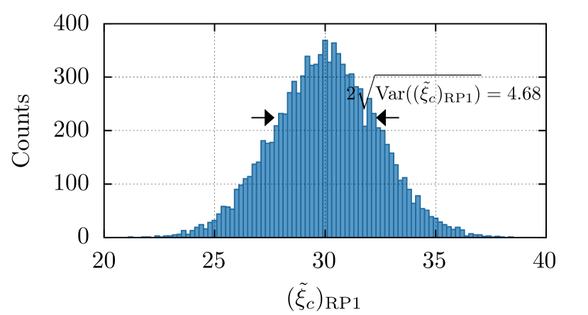
Figure 7: Probability distribution of the estimator $(\tilde{\xi}_{c})_{\text{RP1}}$. The simulation has been performed for the 10-qubit Dicke state $|D_{10,5}\rangle$. $L_{\text{RP1}}=7400$ random pairs have been chosen with $K_{\text{RP1}}=1$ repetitions. The histogram consists of $99$ bins with a size of $0.2$.

The results in Tab. 1 show the smallest variance for the estimator $(\tilde{\xi}_{c})_{\text{TS}}$. $\text{Var}[(\tilde{\xi}_{c})_{\text{TS}}]$ is about two magnitudes smaller than the next bigger variances of the schemes AP1 and RP1. We note that this appears reasonable as in each experimental run only two qubits are measured in the schemes AP1 and RP1. Therefore, in a hand-wavy sense, less information is extracted in each step. The variances of both the schemes AP1 and RP1 are almost the same, in which the value is slightly larger for the scheme AP1. This appears counter-intuitive as the additional randomization in the scheme RP1 is expected to introduce further uncertainty. We note however, that this is due to the slightly less state samples used for the scheme AP1. In case we increase the number of repetitions by one, i.e., $K_{\text{AP1}}=63$, we obtain $\text{Var}[(\tilde{\xi}_{c})_{\text{AP1}}]=5.5163$.

The fact that the variance of $(\tilde{\xi}_{c})_{\text{RP1}}$ is two orders larger then for $(\tilde{\xi}_{c})_{\text{TS}}$ is also revealed in Fig. 7. Fig. 7 shows the histogram of $(\tilde{\xi}_{c})_{\text{RP1}}$ for the Dicke state $\ket{D_{10,5}}$. From Tab. 1, we obtain $2\times\text{Var}[(\tilde{\xi}_{c})_{\text{RP1}}]^{1/2}=4.7195\approx 4.68$. The deviation is attributed to the finite number of repetitions. The histogram in Fig. 7 is obtained from $10000$ samples of $(\tilde{\xi}_{c})_{\text{RP1}}$.

Finally, the variances of the schemes AP2 and RP2 are in turn almost an order larger than the variances of the schemes AP1 and RP1. This seems plausible, as both the schemes AP2 and RP2 rely also on measurements on single qubits and thus less information is revealed from each state sample as compared to the schemes AP1 and RP1. In detail, the variance $\text{Var}[(\tilde{\xi}_{c})_{\text{RP2}}]$ is slightly larger than the variance $\text{Var}[(\tilde{\xi}_{c})_{\text{AP2}}]$, which we attribute to the additional randomness in scheme RP2.

Estimator	$\text{Var}(\tilde{\xi})$	Estimator	$\text{Var}(\tilde{\xi})$
$(\tilde{\xi}_{c})_{\text{TS}}$	$0.0284$
$(\tilde{\xi}_{c})_{\text{AP1}}$	$5.5836$	$(\tilde{\xi}_{c})_{\text{AP2}}$	$24.5046$
$(\tilde{\xi}_{c})_{\text{RP1}}$	$5.5685$	$(\tilde{\xi}_{c})_{\text{RP2}}$	$25.6667$

Table 1: Variances of the estimators for the Dicke state $|D_{10,5}\rangle$. The variances are obtained for $K_{\text{TS}}=7400$, $K_{\text{AP1}}=82$ and $K_{\text{AP2}}=60$. For the randomized approaches we used $L_{\text{RP1}}=7400$ with $K_{\text{RP1}}=1$ and $L_{\text{RP2}}=2775$ with $K_{\text{RP2}}=2$. In this case, the total number of measurements is $22200$ for all schemes except AP1. For the scheme AP1 the total number of state samples is slightly less: $22140$.

	$\xi_{b}$	$\xi_{c}$	$\xi_{d}$
TS	$0$	$\frac{N^{4}+4N^{3}-4N^{2}-16N}{64K_{\text{TS}}}$	$0$
AP1	$\frac{3N\left(K_{\text{AP1}}\mathcal{O}(N^{5})-\mathcal{O}(N^{5})\right)}{16(K_{\text{AP1}}-1)K_{\text{AP1}}(N-1)^{4}}$	$\frac{N\left(K_{\text{AP1}}\mathcal{O}(N^{5})-\mathcal{O}(N^{5})\right)}{32(K_{\text{AP1}}-1)K_{\text{AP1}}(N-1)^{2}}$	$\frac{N\left(K_{\text{AP1}}\mathcal{O}(N^{5})-\mathcal{O}(N^{5})\right)}{16(K_{\text{AP1}}-1)K_{\text{AP1}}(N-1)^{2}}$
AP2	$\frac{9N^{2}-6N}{16K_{\text{AP2}}}$	$\frac{6N^{5}-20N^{4}+25N^{3}-16N^{2}+4N}{32K_{\text{AP2}}(N-1)}$	$\frac{6N^{4}-16N^{3}+15N^{2}-6N}{16K_{\text{AP2}}}$
RP1	$\frac{3N^{3}\left(L_{\text{RP1}}\mathcal{O}(N^{3})+\mathcal{O}(N^{2})\right)}{16(L_{\text{RP1}}-1)L_{\text{RP1}}(N-1)^{2}}$	$\frac{N^{2}\left(L_{\text{RP1}}\mathcal{O}(N^{4})+\mathcal{O}(N^{3})\right)}{32(L_{\text{RP1}}-1)L_{\text{RP1}}}$	$\frac{N^{3}\left(L_{\text{RP1}}\mathcal{O}(N^{3})+\mathcal{O}(N^{2})\right)}{16(L_{\text{RP1}}-1)L_{\text{RP1}}}$
RP2	$\frac{9N^{4}-6N^{3}}{16K_{\text{RP2}}L_{\text{RP2}}}$	$\frac{6N^{6}-16N^{5}+17N^{4}-12N^{3}+4N^{2}}{32K_{\text{RP2}}L_{\text{RP2}}}$	$\frac{6N^{6}-16N^{5}+15N^{4}-6N^{3}}{16K_{\text{RP2}}L_{\text{RP2}}}$

Table 2: Expressions for the variances for specific states. The inequality Eq. (6b) is maximally violated by many-body singlet states in Eq. (8). For this reason, we show the variance for the many-body singlet states. Correspondingly we evaluate the variance of $\tilde{\xi}_{c}$ for the Dicke state $\ket{D_{N,N/2}}$, as this state violates Eq. (6c) the most. Finally, the many-body singlet states also violate Eq. (6d) and the variance for these states is shown in the third column. We note that the variances for the scheme RP1 are given for the case $K_{\text{RP1}}=1$.

IV.2 Scaling of the variances

Next, we will compare the estimators by the scaling of the variances for specific states that violate the spin-squeezing inequalities. On the one hand, we use the many-body singlet state presented in Eq. (8) for the spin-squeezing inequalities in Eq. (6b) and Eq. (6d). Many-body singlet states maximally violate Eq. (6b) and also show a violation of Eq. (6d). On the other hand, the spin-squeezing inequality (6c) is maximally violated by the Dicke state $|D_{N,N/2}\rangle$ defined in Eq. (9). Thus, we analyze the variances of $\xi_{c}$ with the help of the Dicke state.

For the many-body singlet state in Eq. (8), we show the expressions for the variances $\text{Var}[\tilde{\xi}_{b}]$ and $\text{Var}[\tilde{\xi}_{d}]$ in Tab. 2. We observe that for the total spin estimator both $\text{Var}[(\tilde{\xi}_{b})_{\text{TS}}]=0$ and $\text{Var}[(\tilde{\xi}_{d})_{\text{TS}}]=0$. This is due to the properties in Eq. (7). Moreover, Tab. 2 shows that both $\text{Var}[(\tilde{\xi}_{b})_{\text{AP1}}]$ and $\text{Var}[(\tilde{\xi}_{b})_{\text{AP2}}]$ scale as $\mathcal{O}(N^{2})$, whereas $\text{Var}[(\tilde{\xi}_{b})_{\text{RP1}}]$ and $\text{Var}[(\tilde{\xi}_{b})_{\text{RP2}}]$ scale as $\mathcal{O}(N^{4})$. As expected, the variances of the estimator that use random pair correlations scale worse with $N$. We note that the scaling differs in a factor of $N^{2}$, which corresponds to the order of qubit pairs. Alike, we obtain that the variances for the spin-squeezing parameter $\xi_{d}$ scale as $\text{Var}[(\tilde{\xi}_{d})_{\text{AP1}}],\text{Var}[(\tilde{\xi}_{d})_{\text{AP2}}]\sim\mathcal{O}(N^{4})$ and $\text{Var}[(\tilde{\xi}_{d})_{\text{RP1}}],\text{Var}[(\tilde{\xi}_{d})_{\text{RP2}}]\sim\mathcal{O}(N^{6})$. We note that the result differs to the one of $\xi_{b}$ by a factor of $N^{2}$. This is due to the additional factor of $N-1$ in the parameter $\xi_{d}$.

Finally, for the variance of $\xi_{c}$ we consider the Dicke state $|D_{N,N/2}\rangle$. The results in Tab. 2 show that for this case the total spin estimator has a non-zero variance that scales as $\text{Var}[(\tilde{\xi}_{c})_{\text{TS}}]\sim\mathcal{O}(N^{4})$. For the Dicke state, also the variances of the estimator AP1 and AP2 show the same scaling in $N$, i.e. $\text{Var}[(\tilde{\xi}_{c})_{\text{AP1}}],\text{Var}[(\tilde{\xi}_{c})_{\text{AP2}}]\sim\mathcal{O}(N^{4})$. However, we note that each pair has to be measured $K_{\text{AP}}$-times. Thus, in case the variance is considered as a function of the total number of experimental runs, the scaling is $\mathcal{O}(N^{6})$. As for the other parameters, we observe that the variances of the randomized approaches RP1 and RP2 are two orders larger than for the schemes AP1 and AP2. We obtain $\text{Var}[(\tilde{\xi}_{c})_{\text{RP1}}],\text{Var}[(\tilde{\xi}_{c})_{\text{RP2}}]\sim\mathcal{O}(N^{6})$.

IV.3 Statistical test

With the help of the variances, we can now make a statement on the $p$-value and thus on the significance of an experimental result. For this purpose, we use Cantelli’s inequality [35]. Cantelli’s inequality is a bound on the probability that a real-valued random variable $\tilde{\xi}$ exceeds its mean value by an amount $t$, i.e.,

$$\mathbb{P}\left(\tilde{\xi}-\mathbb{E}(\tilde{\xi})\geq t\right)\leq\frac{\text{Var}[\tilde{\xi}]}{\text{Var}[\tilde{\xi}]+t^{2}}.$$ (32)

As we are focused on unbiased estimators, Cantelli’s inequality bounds the probability that the estimator deviates from the actual value $\xi=\mathbb{E}[\tilde{\xi}]$. However, the variances depend on the quantum state. As a result, we have to take the upper bound of the variance over all quantum states.

In this section however, we use a different approach. We consider that the target state is the Dicke state $|D_{N,N/2}\rangle$. In addition, we assume that only depolarisation noise affects the state preparation, i.e. the prepared state has the form

$$\rho=p\outerproduct{D_{N,N/2}}{D_{N,N/2}}+(1-p)\frac{\mathds{1}}{2^{N}},$$ (33)

with $p\in[0,1]$. For $N=10$ qubits, the variances are plotted in Fig. 8. We can observe that for the whole range of $p$, the variances of $(\tilde{\xi_{c}})_{\text{AP1}}$ and $(\tilde{\xi_{c}})_{\text{RP1}}$ are at least two orders of magnitude larger than the variance of $(\tilde{\xi_{c}})_{\text{TS}}$. The variances of $(\tilde{\xi_{c}})_{\text{AP2}}$ and $(\tilde{\xi_{c}})_{\text{RP2}}$ are in turn three orders larger.

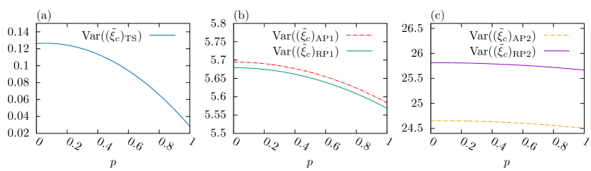
Figure 8: Variances of the estimators $(\tilde{\xi}_{c})_{\text{TS}}$, $(\tilde{\xi}_{c})_{\text{AP1}}$, $(\tilde{\xi}_{c})_{\text{AP2}}$, $(\tilde{\xi}_{c})_{\text{RP1}}$ and $(\tilde{\xi}_{c})_{\text{RP2}}$ for the Dicke state of $N=10$ qubits $|D_{10,5}\rangle$ mixed with depolarisation noise, i.e., $\rho=p\outerproduct{D_{10,5}}{D_{10,5}}+(1-p)\mathds{1}/2^{N}$. The variances are obtained for $K_{\text{TS}}=7400$, $K_{\text{AP1}}=82$, $K_{\text{AP2}}=60$, $L_{\text{RP1}}=7400$ with $K_{\text{RP1}}=1$ and $L_{\text{RP2}}=2775$ with $K_{\text{RP2}}=2$.

Moreover, Fig. 8 shows that the variances take the smallest value for the pure Dicke state, i.e., for $p=1$. What is more, the spin-squeezing inequality in Eq. (6c) detects the mixture $\rho$ as entangled for $p>p^{*}=\frac{N-1}{2N-1}$. For $N=10$, the critical value is $p^{*}=0.47$. As a result, all variances take the maximum in the region of separable states.

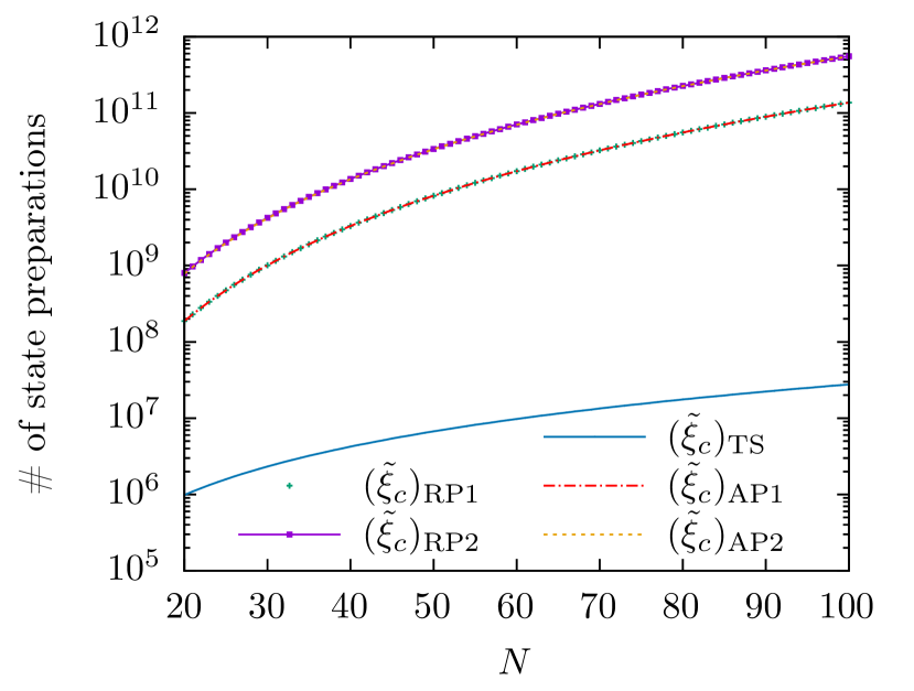
Figure 9: Number of state preparations necessary to verify a violation of Eq. (6c) by $t=0.1\times\frac{N}{2}$ with a significance level of $\gamma=0.95$.

To assess the number of state preparations, we can make use of Cantelli’s inequality in Eq. (32). For this purpose, we use the assumption that the state is always described by the mixture in Eq. (33). Moreover, we use that for any $t>0$, the bound in Cantelli’s inequality is monotonically increasing in the variance. For this reason, we can take the maximum of the variance for the mixture $\rho$. To verify a violation of $t$ by at least a confidence level of $\gamma=1-p$, we can rearrange Cantelli’s inequality to obtain a lower bound for the necessary number of state samples. To be precise, Cantelli’s inequality yields the number of repetitions $K_{\text{TS}}$, $K_{\text{AP1}}$, $K_{\text{AP2}}$ and $L_{\text{RP1}}$ under the assumption that $K_{\text{RP1}}=1$. In addition, we used Cantelli’s inequality to obtain the product $K_{\text{RP2}}L_{\text{RP2}}$ such that the observed violation of $t$ has a confidence of $\gamma$. In Fig. 9, we show the total number of state preparations, i.e., we plot $3K_{\text{TS}}$, $3K_{\text{AP1}}N(N-1)$, $K_{\text{AP2}}N(4N-3)$, $3K_{\text{RP1}}L_{\text{RP1}}$ and $4K_{\text{RP2}}L_{\text{RP2}}$.

The figure shows, that $(\tilde{\xi}_{c})_{\text{TS}}$ requires the least number of state samples. Moreover, the number of state samples that are necessary in the scheme TS scales favourable with $N$ compared to the other schemes. It is interesting to note that the number of required state samples for the schemes AP1, AP2, RP1 and RP2 obeys the same scaling with $N$. For the schemes AP1 and RP1 almost the same number of state samples are needed. This appears reasonable as the variances of both schemes do not differ much as is shown in Fig. 8 (b). More samples are needed for the schemes AP2 and RP2. However, Fig. 8 (c) shows that also the variances of the schemes AP2 and RP2 do not differ by much. The schemes AP2 and RP2 thus require almost the same number of state samples, whereat slightly more state samples are needed for the scheme RP2.

V Conclusion

We have discussed different approaches to estimate spin-squeezing inequalities from experimental data. On the one hand, this includes the straightforward estimation from measurements of the total angular momenta. On the other hand, we have introduced different schemes to estimate spin-squeezing inequalities from pair correlations. In doing so, we have shown that it is also possible to sample the pair correlations at random. By providing different schemes to estimate spin-squeezing inequalities it is possible to choose the most suitable approach for a given experimental set-up.

As the second important point of the paper, we have performed a rigorous error analysis of the schemes. The spin-squeezing inequalities are non-linear in the quantum state and thus are the estimators. We therefore provide an error analysis based on the variances of the estimators and Cantelli’s inequality that can be applied to generic non-linear estimators. Finally, we apply the error analysis to derive the necessary number of measurements to verify a violation of a spin-squeezing inequality with a given confidence level.

Our methods and results will not only be useful for experimental studies on spin-squeezing, they also lead to further research questions worth to study. For instance, one may extend the presented methods to other non-linear figures of merit, such as the purity or entropies of a quantum state. Furthermore, it would be interesting to study the concept of randomly picked subsets of particles also in the context of other methods of quantum state analysis, such as shadow tomography.

The authors would like to thank Kiara Hansenne, Andreas Ketterer, Matthias Kleinmann, Martin Kliesch, René Schwonnek, Géza Tóth, Lina Vandré, and Nikolai Wyderka for useful discussions and comments. This work has been supported by the Deutsche Forschungsgemeinschaft (DFG, German Research Foundation, project numbers 447948357 and 440958198), the Sino-German Center for Research Promotion (Project M-0294), and the German Ministry of Education and Research (Project QuKuK, BMBF Grant No. 16KIS1618K). J.L.B. acknowledges support from the House of Young Talents of the University of Siegen. S.I. acknowledges support from the DAAD.

Appendix A Unbiased estimators

In this appendix, we will prove that the estimators in Sec. III are unbiased. For the total spin estimator, $\widetilde{\langle J_{\alpha}^{2}\rangle}_{\text{TS}}$ is the sample mean and $\widetilde{(\Delta J_{\alpha})^{2}}_{\text{TS}}$ is the sample variance. Hence, the estimators are known to be unbiased [37]. We will therefore focus on the estimators that rely on pair correlations.

A.1 Estimator based on pair correlations

As the term $s_{\alpha}^{(P_{1},k)}s_{\alpha}^{(P_{2},k)}$ is the product of the spins of the qubit pair $P=(P_{1},P_{2})$ in the same measurement repetition $k$, we have for $i\in\{1,2\}$

$$\mathbb{E}\left[s_{\alpha}^{(P_{i},k)}\right]=\frac{1}{2}\langle{\sigma_{\alpha}^{(P_{i})}}\rangle\qquad\text{and}\qquad\mathbb{E}\left[s_{\alpha}^{(P_{1},k)}s_{\alpha}^{(P_{2},k)}\right]=\frac{1}{4}\langle{\sigma_{\alpha}^{(P_{1})}\sigma_{\alpha}^{(P_{2})}}\rangle.$$ (34)

As a result, we obtain

$$\begin{split}\mathbb{E}\left[\widetilde{\expectationvalue{J_{\alpha}^{2}}}_{\text{AP}}\right]=\frac{N}{4}+\sum_{P}\frac{1}{K_{\text{AP}}}\sum_{k=1}^{K_{\text{AP}}}\mathbb{E}\left[s_{\alpha}^{(P_{1},k)}s_{\alpha}^{(P_{2},k)}\right]=\frac{N}{4}+\frac{1}{4}\sum_{P}\langle{\sigma_{\alpha}^{(P_{1})}\sigma_{\alpha}^{(P_{2})}}\rangle=\langle{J_{\alpha}^{2}}\rangle,\end{split}$$ (35)

where we have used that

$$\begin{split}\frac{1}{4}\sum_{P}\langle{\sigma_{\alpha}^{(P_{1})}\sigma_{\alpha}^{(P_{2})}}\rangle=\frac{1}{4}\sum_{P_{1}\neq P_{2}}\langle{\sigma_{\alpha}^{(P_{1})}\sigma_{\alpha}^{(P_{2})}}\rangle=\frac{1}{4}\sum_{P_{1},P_{2}}\langle{\sigma_{\alpha}^{(P_{1})}\sigma_{\alpha}^{(P_{2})}}\rangle-\frac{1}{4}\sum_{P_{1}=P_{2}}\langle{(\sigma_{\alpha}^{(P_{1})})^{2}}\rangle=\langle{J_{\alpha}^{2}}\rangle-\frac{N}{4}.\end{split}$$ (36)

Next, we will show that the estimator for the variance in Eq. (21) is unbiased.

$$\begin{split}\mathbb{E}\left[\widetilde{(\Delta J_{\alpha})^{2}}\right]&=\frac{N}{4}+\frac{1}{K_{\text{AP}}}\sum_{P}\sum_{k}\mathbb{E}\left[s_{\alpha}^{(P_{1},k)}s_{\alpha}^{(P_{2},k)}\right]-\frac{1}{K_{\text{AP}}(K_{\text{AP}}-1)(N-1)^{2}}\sum_{P,Q}\sum_{k\neq l}\mathbb{E}\left[s_{\alpha}^{(P_{1},k)}s_{\alpha}^{(Q_{2},l)}\right]\\ &=\frac{N}{4}+\frac{1}{K_{\text{AP}}}\sum_{P}\sum_{k}\frac{1}{4}\langle{\sigma_{\alpha}^{(P_{1})}\sigma_{\alpha}^{(P_{2})}}\rangle-\frac{1}{K_{\text{AP}}(K_{\text{AP}}-1)(N-1)^{2}}\sum_{P,Q}\sum_{k\neq l}\mathbb{E}\left[s_{\alpha}^{(P_{1},k)}\right]\mathbb{E}\left[s_{\alpha}^{(Q_{2},l)}\right]\\ &=\frac{N}{4}+\sum_{P}\frac{1}{4}\langle{\sigma_{\alpha}^{(P_{1})}\sigma_{\alpha}^{(P_{2})}}\rangle-\frac{1}{K_{\text{AP}}(K_{\text{AP}}-1)(N-1)^{2}}\sum_{P,Q}\sum_{k\neq l}\frac{1}{2}\langle{\sigma_{\alpha}^{(P_{1})}}\rangle\frac{1}{2}\langle{\sigma_{\alpha}^{(Q_{2})}}\rangle\\ &=\langle{J_{\alpha}^{2}}\rangle-\frac{1}{(N-1)^{2}}\Big{(}\sum_{P}\frac{1}{2}\langle{\sigma_{\alpha}^{(P_{1})}}\rangle\Big{)}\Big{(}\sum_{Q}\frac{1}{2}\langle{\sigma_{\alpha}^{(Q_{2})}}\rangle\Big{)}=\langle{J_{\alpha}^{2}}\rangle-\langle{J_{\alpha}}\rangle^{2}=(\Delta J_{\alpha})^{2}\end{split}$$ (37)

In the above calculation, we have used that $\sum_{P}\frac{1}{2}\langle{\sigma_{\alpha}^{(P_{1})}}\rangle=\sum_{P_{1}\neq P_{2}}\frac{1}{2}\langle{\sigma_{\alpha}^{(P_{1})}}\rangle=(N-1)\langle{\sum_{P_{1}}\frac{1}{2}\sigma_{\alpha}^{(P_{1})}}\rangle=(N-1)\langle{J_{\alpha}}\rangle$.

To show that the estimator of $\langle J_{\alpha}\rangle^{2}$ is unbiased, we use that the qubits of each pair $(i,j)$ are measured in different experimental runs. Hence, the outcomes are statistically independent: $\mathbb{E}[s_{\alpha}^{(i,2k)}s_{\alpha}^{(j,2k-1)}]=\mathbb{E}[s_{\alpha}^{(i,2k)}]\mathbb{E}[s_{\alpha}^{(j,2k-1)}]=\frac{1}{4}\langle{\sigma_{\alpha}^{(i)}}\rangle\langle{\sigma_{\alpha}^{(j)}}\rangle$. Thus, the estimator is unbiased:

$$\begin{split}\mathbb{E}\left[\widetilde{\expectationvalue{J_{\alpha}}^{2}}_{\text{AP}}\right]=\sum_{i,j=1}^{N}\frac{1}{\frac{K_{\text{AP}}}{2}}\sum_{k=1}^{\frac{K_{\text{AP}}}{2}}\mathbb{E}[s_{\alpha}^{(i,2k)}s_{\alpha}^{(j,2k-1)}]=\sum_{i,j=1}^{N}\frac{1}{4}\langle{\sigma_{\alpha}^{(i)}}\rangle\langle{\sigma_{\alpha}^{(j)}}\rangle=\langle{\frac{1}{2}\sum_{i=1}^{N}\sigma_{\alpha}^{(i)}}\rangle\langle{\frac{1}{2}\sum_{j=1}^{N}\sigma_{\alpha}^{(j)}}\rangle=\langle{J_{\alpha}}\rangle^{2}.\end{split}$$ (38)

A.2 Estimator based on random pair correlations

We now want to calculate the expectation values of the estimators that make use of random pair correlations. For this, we have to first specify how the expectation value has to be understood. As both the indices of the qubits and the outcomes are random variables, we can calculate the expectation value by the law of iterated expectations. In case, $\mathcal{I}$ is a random variable that takes the values $\mathcal{I}=1,\ldots,N$ with uniform probability, the expectation value of the spin of qubit $\mathcal{I}$ evaluates to

$$\mathbb{E}\left[s_{\alpha}^{(\mathcal{I},k)}\right]=\mathbb{E}_{\mathcal{I}}\left[\mathbb{E}_{s}\left(s_{\alpha}^{(\mathcal{I},k)}\big{|}\mathcal{I}\right)\right]=\mathbb{E}_{\mathcal{I}}\left[\frac{1}{2}\langle{\sigma_{\alpha}^{(\mathcal{I})}}\rangle\right]=\sum_{i=1}^{N}\mathbb{P}(\mathcal{I}=i)\frac{1}{2}\langle{\sigma_{\alpha}^{(i)}}\rangle=\frac{1}{N}\sum_{i=1}^{N}\frac{1}{2}\langle{\sigma_{\alpha}^{(i)}}\rangle=\frac{1}{N}\langle{J_{\alpha}}\rangle.$$ (39)

In the above equation, we used the uniform probability distribution $\mathbb{P}(\mathcal{I}=i)=\frac{1}{N}$. We note that this is indeed the marginal distribution in case we sample uniformly all distinct pairs with the probability distribution in Eq. (26), i.e., $\mathbb{P}(\mathcal{I}=i)=\sum_{j=1}^{N}\mathbb{P}(\mathcal{I}=i,\mathcal{J}=j)=\sum_{j\neq i}^{N}\frac{1}{N(N-1)}=\frac{1}{N}=\mathbb{P}(\mathcal{J}=j)$. Similarly, we can show that

$$\begin{split}\mathbb{E}\left[s_{\alpha}^{(\mathcal{I},k)}s_{\alpha}^{(\mathcal{J},k)}\right]&=\mathbb{E}_{\mathcal{I},\mathcal{J}}\left[\mathbb{E}_{s}\left(s_{\alpha}^{(\mathcal{I},k)}s_{\alpha}^{(\mathcal{J},k)}\bigg{|}\mathcal{I},\mathcal{J}\right)\right]=\mathbb{E}_{\mathcal{I},\mathcal{J}}\left[\frac{1}{4}\langle{\sigma_{\alpha}^{(\mathcal{I})}\sigma_{\alpha}^{(\mathcal{J})}}\rangle\right]\\ &=\sum_{i\neq j}^{N}\mathbb{P}(\mathcal{I}=i,\mathcal{J}=j)\frac{1}{4}\langle{\sigma_{\alpha}^{(i)}\sigma_{\alpha}^{(j)}}\rangle=\sum_{i\neq j}^{N}\frac{1}{N(N-1)}\frac{1}{4}\langle{\sigma_{\alpha}^{(i)}\sigma_{\alpha}^{(j)}}\rangle=\frac{1}{N(N-1)}\left(\langle{J_{\alpha}^{2}}\rangle-\frac{N}{4}\right),\end{split}$$ (40)

where we have used in the third step that only distinct pairs are considered, i.e. $\mathbb{P}(\mathcal{I}=i,\mathcal{J}=i)=0$. We can thus evaluate the expectation value:

$$\begin{split}\mathbb{E}\left[\widetilde{\expectationvalue{J_{\alpha}^{2}}}_{\text{RP}}\right]&=\frac{N}{4}+\frac{N(N-1)}{K_{\text{RP}}L_{\text{RP}}}\sum_{l=1}^{L_{\text{RP}}}\sum_{k=1}^{K_{\text{RP}}}\mathbb{E}\left[s_{\alpha}^{(\mathcal{I}_{l},k)}s_{\alpha}^{(\mathcal{J}_{l},k)}\right]=\frac{N}{4}+\frac{N(N-1)}{K_{\text{RP}}L_{\text{RP}}}\sum_{l=1}^{L_{\text{RP}}}\sum_{k=1}^{K_{\text{RP}}}\frac{1}{N(N-1)}\left(\langle{J_{\alpha}^{2}}\rangle-\frac{N}{4}\right)=\langle{J_{\alpha}^{2}}\rangle.\end{split}$$ (41)

To calculate the expectation value of the estimator $\widetilde{(\Delta J_{\alpha})^{2}}_{\text{RP}}$, we use Eq. (40) and apply that the product in the last term of the estimator only involves independent random variables:

$$\begin{split}&\mathbb{E}\left[\widetilde{(\Delta J_{\alpha})^{2}}_{\text{RP}}\right]=\frac{N}{4}+\frac{N(N-1)}{L_{\text{RP}}K_{\text{RP}}}\sum_{l=1}^{L_{\text{RP}}}\sum_{k=1}^{K_{\text{RP}}}\mathbb{E}\left[s_{\alpha}^{(\mathcal{I}_{l},k)}s_{\alpha}^{(\mathcal{J}_{l},k)}\right]-\frac{N^{2}}{L_{\text{RP}}(L_{\text{RP}}-1)K_{\text{RP}}^{2}}\sum_{l\neq m}^{L_{\text{RP}}}\sum_{k,q=1}^{K_{\text{RP}}}\mathbb{E}\left[s_{\alpha}^{(\mathcal{I}_{l},k)}\right]\mathbb{E}\left[s_{\alpha}^{(\mathcal{J}_{m},q)}\right]\\ =&\frac{N}{4}+\frac{N(N-1)}{L_{\text{RP}}K_{\text{RP}}}\sum_{l=1}^{L_{\text{RP}}}\sum_{k=1}^{K_{\text{RP}}}\frac{1}{N(N-1)}\left(\langle{J_{\alpha}^{2}}\rangle-\frac{N}{4}\right)-\frac{N^{2}}{L_{\text{RP}}(L_{\text{RP}}-1)K_{\text{RP}}^{2}}\sum_{l\neq m}^{L_{\text{RP}}}\sum_{k,q=1}^{K_{\text{RP}}}\frac{1}{N^{2}}\langle{J_{\alpha}}\rangle^{2}\\ =&\langle{J_{\alpha}^{2}}\rangle-\langle{J_{\alpha}}\rangle^{2}=(\Delta J_{\alpha})^{2}.\end{split}$$ (42)

Similarly, we can show for the estimator of $\langle{J_{\alpha}}\rangle^{2}$ for scheme RP2 that

$$\begin{split}\mathbb{E}\left[\widetilde{\expectationvalue{J_{\alpha}}^{2}}_{\text{RP}}\right]&=\frac{2N^{2}}{K_{\text{RP}}L_{\text{RP}}}\sum_{l=1}^{L_{\text{RP}}}\sum_{k=1}^{\frac{K_{\text{RP}}}{2}}\mathbb{E}[s_{\alpha}^{(\mathcal{I}_{l},2k)}]\mathbb{E}[s_{\alpha}^{(\mathcal{J}_{l},2k-1)}]=\frac{2N^{2}}{K_{\text{RP}}L_{\text{RP}}}\sum_{l=1}^{L_{\text{RP}}}\sum_{k=1}^{\frac{K_{\text{RP}}}{2}}\frac{1}{N^{2}}\langle{J_{\alpha}}\rangle^{2}=\langle{J_{\alpha}}\rangle^{2}.\end{split}$$ (43)

Here, we used again that the outcomes of each pair $(i,j)$ are obtained from different experimental runs and are thus independent. Moreover, all pairs are considered with uniform probability, such that also the random variables $\mathcal{I},\mathcal{J}$ are independent.

Appendix B Derivation of the variances

B.1 Estimator based on the total spin

The variances of the estimators can be derived from the variances of the parts. Thus, we are going to derive the variances $\text{Var}[\widetilde{\langle{J_{\alpha}^{2}}\rangle}_{\text{TS}}]=\mathbb{E}[(\widetilde{\langle{J_{\alpha}^{2}}\rangle}_{\text{TS}})^{2}]-(\mathbb{E}[\widetilde{\langle{J_{\alpha}^{2}}\rangle}])^{2}$ and $\text{Var}[\widetilde{(\Delta J_{\alpha})^{2}}_{\text{TS}}]=\mathbb{E}[(\widetilde{(\Delta J_{\alpha})^{2}}_{\text{TS}})^{2}]-\mathbb{E}[\widetilde{(\Delta J_{\alpha})^{2}}_{\text{TS}}]^{2}$.

For a clear arrangement of the calculation, we will apply a graphical representation. We use the first expression to explain the representation.

$$\begin{split}\mathbb{E}\left[(\widetilde{\langle{J_{\alpha}^{2}}\rangle}_{\text{TS}})^{2}\right]=\mathbb{E}\left[\left(\sum_{k=1}^{K_{\text{TS}}}\frac{(m_{\alpha}^{(k)})^{2}}{K_{\text{TS}}}\right)^{2}\right]=&\frac{1}{K_{\text{TS}}^{2}}\sum_{k_{1},k_{2}=1}^{K_{\text{TS}}}\mathbb{E}\left[(m_{\alpha}^{(k_{1})})^{2}(m_{\alpha}^{(k_{2})})^{2}\right]\\ =&\frac{1}{K_{\text{TS}}^{2}}\sum_{k_{1}\neq k_{2}=1}^{K_{\text{TS}}}\mathbb{E}\left[(m_{\alpha}^{(k_{1})})^{2}(m_{\alpha}^{(k_{2})})^{2}\right]+\frac{1}{K_{\text{TS}}^{2}}\sum_{k_{1}=k_{2}=1}^{K_{\text{TS}}}\mathbb{E}\left[(m_{\alpha}^{(k_{1})})^{4}\right]\\ &\hskip 56.9055pt\leavevmode\hbox to43.44pt{\vbox to23.01pt{\text{[drawing]}}}\hskip 39.83368pt+\hskip 56.9055pt\leavevmode\hbox to43.44pt{\vbox to28.25pt{\text{[drawing]}}}\\ =&\frac{K_{\text{TS}}-1}{K_{\text{TS}}}\langle{J_{\alpha}^{2}}\rangle^{2}+\frac{1}{K_{\text{TS}}}\langle{J_{\alpha}^{4}}\rangle\end{split} k_{1} k_{2} k_{1} k_{2} k_{1} k_{2} k_{1} k_{2}$$ (44)

In the above derivation, we consider the terms with $k_{1}\neq k_{2}$ separately as the outcomes are obtained in different experimental runs and thus $\mathbb{E}[(m_{\alpha}^{(k_{1})})^{2}(m_{\alpha}^{(k_{2})})^{2}]=\mathbb{E}[(m_{\alpha}^{(k_{1})})^{2}]\mathbb{E}[(m_{\alpha}^{(k_{2})})^{2}]=\langle{J_{\alpha}^{2}}\rangle^{2}$. For terms with more indices it becomes tedious to write down all possibilities for the indices to coincide. Therefore, we will use the graphical representation instead. Two indices are connected if and only if they coincide. With Eq.(44), we can evaluate the variance

$$\begin{split}\text{Var}\left(\widetilde{\langle{J_{\alpha}^{2}}\rangle}_{\text{TS}}\right)=&\mathbb{E}[(\widetilde{\langle{J_{\alpha}^{2}}\rangle}_{\text{TS}})^{2}]-(\mathbb{E}[\widetilde{\langle{J_{\alpha}^{2}}\rangle}])^{2}=\frac{K_{\text{TS}}-1}{K_{\text{TS}}}\langle{J_{\alpha}^{2}}\rangle^{2}+\frac{1}{K_{\text{TS}}}\langle{J_{\alpha}^{4}}\rangle-\langle{J_{\alpha}^{2}}\rangle^{2}=\frac{1}{K_{\text{TS}}}\left(\langle{J_{\alpha}^{4}}\rangle-\langle{J_{\alpha}^{2}}\rangle^{2}\right)\\ =&\frac{1}{K_{\text{TS}}}\left(\Delta J_{\alpha}^{2}\right)^{2}.\end{split}$$ (45)

Next, we will derive the variance of $\widetilde{(\Delta J_{\alpha})^{2}}_{\text{TS}}$.

$$\begin{split}\mathbb{E}\left\{\left[\widetilde{(\Delta J_{\alpha})^{2}}_{\text{TS}}\right]^{2}\right\}=&\mathbb{E}\left\{\left[\frac{1}{K_{\text{TS}}-1}\sum_{k_{1}=1}^{K_{\text{TS}}}\left(m_{\alpha}^{(k_{1})}-\sum_{k_{2}=1}^{K}\frac{m_{\alpha}^{(k_{2})}}{K_{\text{TS}}}\right)^{2}\right]^{2}\right\}\\ =&\frac{1}{(K_{\text{TS}}-1)^{2}}\left\{\sum_{k_{1},k_{2}=1}^{K_{\text{TS}}}\mathbb{E}\left[\left(m_{\alpha}^{(k_{1})}\right)^{2}\left(m_{\alpha}^{(k_{2})}\right)^{2}\right]-\frac{2}{K_{\text{TS}}}\sum_{k_{1},k_{2},k_{3}=1}^{K_{\text{TS}}}\mathbb{E}\left[\left(m_{\alpha}^{(k_{1})}\right)^{2}m_{\alpha}^{(k_{2})}m_{\alpha}^{(k_{3})}\right]\right.\\ &\hskip 49.79231pt\left.+\frac{1}{K_{\text{TS}}^{2}}\sum_{k_{1},k_{2},k_{3},k_{4}=1}^{K_{\text{TS}}}\mathbb{E}\left[m_{\alpha}^{(k_{1})}m_{\alpha}^{(k_{2})}m_{\alpha}^{(k_{3})}m_{\alpha}^{(k_{4})}\right]\right\}.\end{split}$$ (46)

To evaluate the expression above, we apply the graphical representation to the sums. We obtain

$$\sum_{k_{1},k_{2}=1}^{K_{\text{TS}}}\mathbb{E}\left[\left(m_{\alpha}^{(k_{1})}\right)^{2}\left(m_{\alpha}^{(k_{2})}\right)^{2}\right]=\leavevmode\hbox to29.21pt{\vbox to23.01pt{\text{[drawing]}}}+\leavevmode\hbox to29.21pt{\vbox to28.25pt{\text{[drawing]}}}=K_{\text{TS}}(K_{\text{TS}}-1)\langle{J_{\alpha}^{2}}\rangle^{2}+K_{\text{TS}}\langle{J_{\alpha}^{4}}\rangle, k_{1} k_{2} k_{1} k_{2} k_{1} k_{2} k_{1} k_{2}$$ (47)

$$\sum_{k_{1},k_{2},k_{3}=1}^{K}\mathbb{E}\left[\left(m_{\alpha}^{(k_{1})}\right)^{2}m_{\alpha}^{(k_{2})}m_{\alpha}^{(k_{3})}\right]=\begin{aligned} &\leavevmode\hbox to57.67pt{\vbox to23.01pt{\text{[drawing]}}}+\leavevmode\hbox to57.67pt{\vbox to28.25pt{\text{[drawing]}}}+\leavevmode\hbox to57.67pt{\vbox to28.25pt{\text{[drawing]}}}+\leavevmode\hbox to57.67pt{\vbox to28.25pt{\text{[drawing]}}}+\leavevmode\hbox to57.67pt{\vbox to28.25pt{\text{[drawing]}}}\\ &=K_{\text{TS}}(K_{\text{TS}}-1)(K_{\text{TS}}-2)\expectationvalue{J_{\alpha}^{2}}\expectationvalue{J_{\alpha}}^{2}+K_{\text{TS}}(K_{\text{TS}}-1)\expectationvalue{J_{\alpha}^{2}}^{2}+2K_{\text{TS}}(K_{\text{TS}}-1)\expectationvalue{J_{\alpha}^{3}}\expectationvalue{J_{\alpha}}+K_{\text{TS}}\expectationvalue{J_{\alpha}^{4}}\end{aligned} k_{1} k_{1} k_{2} k_{3} k_{1} k_{1} k_{2} k_{3} k_{1} k_{1} k_{2} k_{3} k_{1} k_{1} k_{2} k_{3} k_{1} k_{1} k_{2} k_{3} k_{1} k_{1} k_{2} k_{3} k_{1} k_{1} k_{2} k_{3} k_{1} k_{1} k_{2} k_{3} k_{1} k_{1} k_{2} k_{3} k_{1} k_{1} k_{2} k_{3}$$ (48)

and

$$\sum_{k_{1},k_{2},k_{3},k_{4}=1}^{K}\mathbb{E}\left[m_{\alpha}^{(k_{1})}m_{\alpha}^{(k_{2})}m_{\alpha}^{(k_{3})}m_{\alpha}^{(k_{4})}\right]=\begin{aligned} &\leavevmode\hbox to57.67pt{\vbox to23.01pt{\text{[drawing]}}}\\ &+\leavevmode\hbox to57.67pt{\vbox to28.25pt{\text{[drawing]}}}+\leavevmode\hbox to57.67pt{\vbox to28.25pt{\text{[drawing]}}}+\leavevmode\hbox to57.67pt{\vbox to28.25pt{\text{[drawing]}}}+\leavevmode\hbox to57.67pt{\vbox to28.25pt{\text{[drawing]}}}+\leavevmode\hbox to57.67pt{\vbox to28.25pt{\text{[drawing]}}}+\leavevmode\hbox to57.67pt{\vbox to28.25pt{\text{[drawing]}}}\\ &+\leavevmode\hbox to57.67pt{\vbox to28.25pt{\text{[drawing]}}}+\leavevmode\hbox to57.67pt{\vbox to33.94pt{\text{[drawing]}}}+\leavevmode\hbox to57.67pt{\vbox to33.94pt{\text{[drawing]}}}\\ &+\leavevmode\hbox to57.67pt{\vbox to28.25pt{\text{[drawing]}}}+\leavevmode\hbox to57.67pt{\vbox to28.25pt{\text{[drawing]}}}+\leavevmode\hbox to57.67pt{\vbox to28.25pt{\text{[drawing]}}}+\leavevmode\hbox to57.67pt{\vbox to28.25pt{\text{[drawing]}}}+\leavevmode\hbox to57.67pt{\vbox to28.25pt{\text{[drawing]}}}\\ &=K_{\text{TS}}(K_{\text{TS}}-1)(K_{\text{TS}}-2)(K_{\text{TS}}-3)\expectationvalue{J_{\alpha}}^{4}+6K_{\text{TS}}(K_{\text{TS}}-1)(K_{\text{TS}}-2)\expectationvalue{J_{\alpha}^{2}}\expectationvalue{J_{\alpha}}^{2}+3K_{\text{TS}}(K_{\text{TS}}-1)\expectationvalue{J_{\alpha}^{2}}^{2}\\ &+4K_{\text{TS}}(K_{\text{TS}}-1)\expectationvalue{J_{\alpha}^{3}}\expectationvalue{J_{\alpha}}+K_{\text{TS}}\expectationvalue{J_{\alpha}^{4}}.\end{aligned} k_{1} k_{2} k_{3} k_{4} k_{1} k_{2} k_{3} k_{4} k_{1} k_{2} k_{3} k_{4} k_{1} k_{2} k_{3} k_{4} k_{1} k_{2} k_{3} k_{4} k_{1} k_{2} k_{3} k_{4} k_{1} k_{2} k_{3} k_{4} k_{1} k_{2} k_{3} k_{4} k_{1} k_{2} k_{3} k_{4} k_{1} k_{2} k_{3} k_{4} k_{1} k_{2} k_{3} k_{4} k_{1} k_{2} k_{3} k_{4} k_{1} k_{2} k_{3} k_{4} k_{1} k_{2} k_{3} k_{4} k_{1} k_{2} k_{3} k_{4} k_{1} k_{2} k_{3} k_{4} k_{1} k_{2} k_{3} k_{4} k_{1} k_{2} k_{3} k_{4} k_{1} k_{2} k_{3} k_{4} k_{1} k_{2} k_{3} k_{4} k_{1} k_{2} k_{3} k_{4} k_{1} k_{2} k_{3} k_{4} k_{1} k_{2} k_{3} k_{4} k_{1} k_{2} k_{3} k_{4} k_{1} k_{2} k_{3} k_{4} k_{1} k_{2} k_{3} k_{4} k_{1} k_{2} k_{3} k_{4} k_{1} k_{2} k_{3} k_{4} k_{1} k_{2} k_{3} k_{4} k_{1} k_{2} k_{3} k_{4}$$ (49)

This finally yields

$$\begin{split}\mathbb{E}&\left[\left(\widetilde{(\Delta J_{\alpha})^{2}}_{\text{TS}}\right)^{2}\right]=\frac{1}{(K_{\text{TS}}-1)^{2}}\bigg{[}(K_{\text{TS}}(K_{\text{TS}}-1)\langle{J_{\alpha}^{2}}\rangle^{2}+K_{\text{TS}}\langle{J_{\alpha}^{4}}\rangle\\ &-\frac{2}{K_{\text{TS}}}\left(K_{\text{TS}}(K_{\text{TS}}-1)(K_{\text{TS}}-2)\expectationvalue{J_{\alpha}^{2}}\expectationvalue{J_{\alpha}}^{2}+K_{\text{TS}}(K_{\text{TS}}-1)\expectationvalue{J_{\alpha}^{2}}^{2}+2K_{\text{TS}}(K_{\text{TS}}-1)\expectationvalue{J_{\alpha}^{3}}\expectationvalue{J_{\alpha}}+K_{\text{TS}}\expectationvalue{J_{\alpha}^{4}}\right)\\ &+\frac{1}{K_{\text{TS}}^{2}}\left(K_{\text{TS}}(K_{\text{TS}}-1)(K_{\text{TS}}-2)(K_{\text{TS}}-3)\expectationvalue{J_{\alpha}}^{4}+6K_{\text{TS}}(K_{\text{TS}}-1)(K_{\text{TS}}-2)\expectationvalue{J_{\alpha}^{2}}\expectationvalue{J_{\alpha}}^{2}+3K_{\text{TS}}(K_{\text{TS}}-1)\expectationvalue{J_{\alpha}^{2}}^{2}\right.\\ &\hskip 28.45274pt\left.+4K_{\text{TS}}(K_{\text{TS}}-1)\expectationvalue{J_{\alpha}^{3}}\expectationvalue{J_{\alpha}}+K_{\text{TS}}\expectationvalue{J_{\alpha}^{4}}\right)\bigg{]}\\ =&\frac{1}{K_{\text{TS}}}\expectationvalue{J_{\alpha}^{4}}-\frac{4}{K_{\text{TS}}}\expectationvalue{J_{\alpha}^{3}}\expectationvalue{J_{\alpha}}+\frac{(K_{\text{TS}}-1)^{2}+2}{K_{\text{TS}}(K_{\text{TS}}-1)}\expectationvalue{J_{\alpha}^{2}}^{2}-2\frac{(K_{\text{TS}}-2)(K_{\text{TS}}-3)}{K_{\text{TS}}(K_{\text{TS}}-1)}\expectationvalue{J_{\alpha}^{2}}\expectationvalue{J_{\alpha}}^{2}\\ &+\frac{(K_{\text{TS}}-2)(K_{\text{TS}}-3)}{K_{\text{TS}}(K_{\text{TS}}-1)}\expectationvalue{J_{\alpha}}^{4}.\end{split}$$ (50)

As a result, we arrive at the variance

$$\begin{split}&\text{Var}\left(\widetilde{(\Delta J_{\alpha})^{2}}_{\text{TS}}\right)=\mathbb{E}\left[\left(\widetilde{(\Delta J_{\alpha})^{2}}_{\text{TS}}\right)^{2}\right]-\left(\mathbb{E}\left[\widetilde{(\Delta J_{\alpha})^{2}}_{\text{TS}}\right]\right)^{2}\\ =&\frac{1}{K_{\text{TS}}}\expectationvalue{J_{\alpha}^{4}}-\frac{4}{K_{\text{TS}}}\expectationvalue{J_{\alpha}^{3}}\expectationvalue{J_{\alpha}}+\frac{(K_{\text{TS}}-1)^{2}+2}{K_{\text{TS}}(K_{\text{TS}}-1)}\expectationvalue{J_{\alpha}^{2}}^{2}-2\frac{(K_{\text{TS}}-2)(K_{\text{TS}}-3)}{K_{\text{TS}}(K_{\text{TS}}-1)}\expectationvalue{J_{\alpha}^{2}}\expectationvalue{J_{\alpha}}^{2}\\ &+\frac{(K_{\text{TS}}-2)(K_{\text{TS}}-3)}{K_{\text{TS}}(K_{\text{TS}}-1)}\expectationvalue{J_{\alpha}}^{4}-\left(\left(\Delta J_{\alpha}\right)^{2}\right)^{2}\\ =&\frac{1}{K_{\text{TS}}}\expectationvalue{J_{\alpha}^{4}}-\expectationvalue{J_{\alpha}^{2}}^{2}-\frac{4}{K_{\text{TS}}}\expectationvalue{J_{\alpha}^{3}}\expectationvalue{J_{\alpha}}+\frac{(K_{\text{TS}}-1)^{2}+2}{K_{\text{TS}}(K_{\text{TS}}-1)}\expectationvalue{J_{\alpha}^{2}}^{2}\\ &-2\frac{(K_{\text{TS}}-2)(K_{\text{TS}}-3)-K_{\text{TS}}(K_{\text{TS}}-1)}{K_{\text{TS}}(K_{\text{TS}}-1)}\expectationvalue{J_{\alpha}^{2}}\expectationvalue{J_{\alpha}}^{2}+\frac{(K_{\text{TS}}-2)(K_{\text{TS}}-3)-K_{\text{TS}}(K_{\text{TS}}-1)}{K_{\text{TS}}(K_{\text{TS}}-1)}\expectationvalue{J_{\alpha}}^{4}\\ =&\frac{1}{K_{\text{TS}}}(\Delta J_{\alpha}^{2})^{2}-\frac{K_{\text{TS}}-1}{K_{\text{TS}}}\expectationvalue{J_{\alpha}^{2}}^{2}-\frac{4}{K_{\text{TS}}}\expectationvalue{J_{\alpha}^{3}}\expectationvalue{J_{\alpha}}+\frac{(K_{\text{TS}}-1)^{2}+2}{K_{\text{TS}}(K_{\text{TS}}-1)}\expectationvalue{J_{\alpha}^{2}}^{2}\\ &+4\frac{2K_{\text{TS}}-3}{K_{\text{TS}}(K_{\text{TS}}-1)}\expectationvalue{J_{\alpha}^{2}}\expectationvalue{J_{\alpha}}^{2}-2\frac{2K_{\text{TS}}-3}{K_{\text{TS}}(K_{\text{TS}}-1)}\expectationvalue{J_{\alpha}}^{4}\\ =&\frac{1}{K_{\text{TS}}}(\Delta J_{\alpha}^{2})^{2}-\frac{4}{K_{\text{TS}}}\expectationvalue{J_{\alpha}^{3}}\expectationvalue{J_{\alpha}}+\frac{2}{K_{\text{TS}}(K_{\text{TS}}-1)}\expectationvalue{J_{\alpha}^{2}}^{2}+4\frac{2K_{\text{TS}}-3}{K_{\text{TS}}(K_{\text{TS}}-1)}\expectationvalue{J_{\alpha}^{2}}\expectationvalue{J_{\alpha}}^{2}-2\frac{2K_{\text{TS}}-3}{K_{\text{TS}}(K_{\text{TS}}-1)}\expectationvalue{J_{\alpha}}^{4}\end{split}$$ (51)

We note that the above expression coincides with [37]. As the measurements in $x$-, $y$- and $z$-direction are obtained in independent experimental runs, the different estimators are statistically independent. We can thus write the variance as the sum of the variances of the individual terms. Thereby, we can derive the variances of the spin-squeezing parameters from the above expressions. As an example, we derive the variance of $(\tilde{\xi}_{c})_{\text{TS}}$ that is given in the main text in Eq. (31).

$$\begin{split}\text{Var}\left((\tilde{\xi}_{c})_{\text{TS}}\right)=&\text{Var}\left(\widetilde{\langle{J_{x}^{2}}\rangle}_{\text{TS}}+\widetilde{\langle{J_{y}^{2}}\rangle}_{\text{TS}}-(N-1)\widetilde{(\Delta J_{z})^{2}}_{\text{TS}}\right)\\ =&\text{Var}\left(\widetilde{\langle{J_{x}^{2}}\rangle}_{\text{TS}}\right)+\text{Var}\left(\widetilde{\langle{J_{y}^{2}}\rangle}_{\text{TS}}\right)+\text{Var}\left(-(N-1)\widetilde{(\Delta J_{z})^{2}}_{\text{TS}}\right)\\ =&\text{Var}\left(\widetilde{\langle{J_{x}^{2}}\rangle}_{\text{TS}}\right)+\text{Var}\left(\widetilde{\langle{J_{y}^{2}}\rangle}_{\text{TS}}\right)+(N-1)^{2}\text{Var}\left(\widetilde{(\Delta J_{z}^{2})}_{\text{TS}}\right)\\ =&\frac{1}{K_{\text{TS}}}\left[\left(\Delta J_{x}^{2}\right)^{2}+\left(\Delta J_{y}^{2}\right)^{2}+(N-1)^{2}\left(\Delta J_{z}^{2}\right)^{2}\right.\\ &\quad\left.+(N-1)^{2}\left(-4\expectationvalue{J_{\alpha}^{3}}\expectationvalue{J_{\alpha}}+\frac{2}{K_{\text{TS}}-1}\expectationvalue{J_{\alpha}^{2}}^{2}+4\frac{2K_{\text{TS}}-3}{K_{\text{TS}}-1}\expectationvalue{J_{\alpha}^{2}}\expectationvalue{J_{\alpha}}^{2}-2\frac{2K_{\text{TS}}-3}{K_{\text{TS}}-1}\expectationvalue{J_{\alpha}}^{4}\right)\right].\end{split}$$ (52)

In the above calculation, we used that the estimators $\widetilde{\langle{J_{x}^{2}}\rangle}^{2}_{\text{TS}}$, $\widetilde{\langle{J_{y}^{2}}\rangle}^{2}_{\text{TS}}$ and $\widetilde{(\Delta J_{z}^{2})}_{\text{TS}}$ are statistically independent.

B.2 Estimator based on pair correlations

We are going to derive the variances of $\widetilde{\expectationvalue{J_{\alpha}^{2}}}_{\text{AP}}$, $\widetilde{(\Delta J_{\alpha})^{2}}_{\text{AP}}$ and $\widetilde{\expectationvalue{J_{\alpha}}^{2}}_{\text{AP}}$. As a result, this allows us to obtain the variances of the spin-squeezing parameters. We start with the variance of the estimator $\widetilde{\expectationvalue{J_{\alpha}^{2}}}_{\text{AP}}$ in Eq. (20). As the constant term does not contribute and the second term is a sum of independent random variables, we obtain

$$\begin{split}\text{Var}\left(\widetilde{\expectationvalue{J_{\alpha}^{2}}}_{\text{AP}}\right)=\text{Var}\left(\frac{N}{4}+\frac{1}{K_{\text{AP}}}\sum_{P}\sum_{k=1}^{K_{\text{AP}}}s_{\alpha}^{(P_{1},k)}s_{\alpha}^{(P_{2},k)}\right)=\frac{1}{K_{\text{AP}}^{2}}\sum_{P}\sum_{k=1}^{K_{\text{AP}}}\text{Var}\left(s_{\alpha}^{(P_{1},k)}s_{\alpha}^{(P_{2},k)}\right).\end{split}$$ (53)

With the help of Eq. (34) and

$$\mathbb{E}\left[\left(s_{\alpha}^{(P_{1},k)}s_{\alpha}^{(P_{2},k)}\right)^{2}\right]=\frac{1}{16}\langle{(\sigma_{\alpha}^{(P_{1})})^{2}(\sigma_{\alpha}^{(P_{2})})^{2}}\rangle=\frac{1}{16},$$ (54)

we can evaluate the variances of the individual terms:

$$\begin{split}\text{Var}\left(s_{\alpha}^{(P_{1},k)}s_{\alpha}^{(P_{2},k)}\right)=&\mathbb{E}\left[\left(s_{\alpha}^{(P_{1},k)}s_{\alpha}^{(P_{2},k)}\right)^{2}\right]-\mathbb{E}\left[s_{\alpha}^{(P_{1},k)}s_{\alpha}^{(P_{2},k)}\right]^{2}=\frac{1}{16}\left(1-\langle{\sigma_{\alpha}^{(P_{1})}\sigma_{\alpha}^{(P_{2})}}\rangle^{2}\right).\end{split}$$ (55)

As a result, we obtain

$$\begin{split}\text{Var}\left(\widetilde{\expectationvalue{J_{\alpha}^{2}}}_{\text{AP}}\right)=\frac{1}{K_{\text{AP}}^{2}}\sum_{P}\sum_{k=1}^{K_{\text{AP}}}\frac{1}{16}\left(1-\langle{\sigma_{\alpha}^{(P_{1})}\sigma_{\alpha}^{(P_{2})}}\rangle^{2}\right)=\frac{1}{16K_{\text{AP}}}\left(N(N-1)-\sum_{i\neq j}\langle{\sigma_{\alpha}^{(i)}\sigma_{\alpha}^{(j)}}\rangle^{2}\right),\end{split}$$ (56)

where we made it explicit that the sum over all pairs $P=(i,j)$ only contains distinct pairs $i\neq j$.

To determine the variance of the estimator $\widetilde{(\Delta J_{\alpha})^{2}}_{\text{AP}}$ in Eq. (21), we use Bienaymé’s identity [38]:

$$\begin{split}\text{Var}\left(\widetilde{(\Delta J_{\alpha})^{2}}_{\text{AP}}\right)=&\text{Var}\left(\frac{N}{4}+\frac{1}{K_{\text{AP}}}\sum_{P}\sum_{k=1}^{K_{\text{AP}}}s_{\alpha}^{(P_{1},k)}s_{\alpha}^{(P_{2},k)}-\frac{1}{K_{\text{AP}}(K_{\text{AP}}-1)(N-1)^{2}}\sum_{P,Q}\sum_{k\neq l}^{K_{\text{AP}}}s_{\alpha}^{(P_{1},k)}s_{\alpha}^{(Q_{2},l)}\right)\\ =&\frac{1}{K_{\text{AP}}^{2}}\sum_{P}\sum_{k=1}^{K_{\text{AP}}}\text{Var}\left(s_{\alpha}^{(P_{1},k)}s_{\alpha}^{(P_{2},k)}\right)+\frac{1}{K_{\text{AP}}^{2}(K_{\text{AP}}-1)^{2}(N-1)^{4}}\text{Var}\left(\sum_{P,Q}\sum_{k\neq l}^{K_{\text{AP}}}s_{\alpha}^{(P_{1},k)}s_{\alpha}^{(Q_{2},l)}\right)\\ &-\frac{2}{K_{\text{AP}}^{2}(K_{\text{AP}}-1)(N-1)^{2}}\text{Cov}\left(\sum_{P}\sum_{k=1}^{K_{\text{AP}}}s_{\alpha}^{(P_{1},k)}s_{\alpha}^{(P_{2},k)},\sum_{P,Q}\sum_{k\neq l}^{K_{\text{AP}}}s_{\alpha}^{(P_{1},k)}s_{\alpha}^{(Q_{2},l)}\right).\end{split}$$ (57)

In the above expression, we applied that the constant term does not contribute to the variance. Moreover, the random variables in the first sum are statistically independent, such that the variance of the sum is just the sum of the variances. The variance can be obtained by plugging in the expressions

$$\begin{split}&\text{Var}\left(s_{\alpha}^{(P_{1},k)}s_{\alpha}^{(P_{2},k)}\right)=\frac{1}{16}\left(1-\langle{\sigma_{\alpha}^{(P_{1})}\sigma_{\alpha}^{(P_{2})}}\rangle^{2}\right),\\ &\text{Var}\left(\sum_{P,Q}\sum_{k\neq l}^{K_{\text{AP}}}s_{\alpha}^{(P_{1},k)}s_{\alpha}^{(Q_{2},l)}\right)=K_{\text{AP}}(K_{\text{AP}}-1)(K_{\text{AP}}-2)(K_{\text{AP}}-3)(N-1)^{4}\langle{J_{\alpha}}\rangle^{4}\\ &\hskip 28.45274pt+K_{\text{AP}}(K_{\text{AP}}-1)(K_{\text{AP}}-2)(N-1)^{2}\langle{J_{\alpha}}\rangle^{2}\Bigg{[}2(N-1)\left((N-1)\langle{J_{\alpha}}\rangle^{2}+\frac{N}{4}-\sum_{i=1}^{N}\frac{1}{4}\langle{\sigma_{\alpha}^{(i)}}\rangle^{2}\right)\\ &\hskip 213.39566pt+2\left(\langle{J_{\alpha}^{2}}\rangle+N(N-2)\langle{J_{\alpha}}\rangle^{2}-\frac{N}{4}+\sum_{i=1}^{N}\frac{1}{4}\langle{\sigma_{\alpha}^{(i)}}\rangle^{2}\right)\Bigg{]}\\ &\hskip 28.45274pt+K_{\text{AP}}(K_{\text{AP}}-1)\Bigg{[}(N-1)^{2}\left((N-1)\langle{J_{\alpha}}\rangle^{2}+\frac{N}{4}-\sum_{i=1}^{N}\frac{1}{4}\langle{\sigma_{\alpha}^{(i)}}\rangle^{2}\right)^{2}\\ &\hskip 113.81102pt+\left(\langle{J_{\alpha}^{2}}\rangle+N(N-2)\langle{J_{\alpha}}\rangle^{2}-\frac{N}{4}+\sum_{i=1}^{N}\frac{1}{4}\langle{\sigma_{\alpha}^{(i)}}\rangle^{2}\right)^{2}\Bigg{]}\\ &\hskip 56.9055pt-K_{\text{AP}}^{2}(K_{\text{AP}}-1)^{2}(N-1)^{4}\langle{J_{\alpha}}\rangle^{4},\\ &\text{Cov}\left(\sum_{P}\sum_{k=1}^{K_{\text{AP}}}s_{\alpha}^{(P_{1},k)}s_{\alpha}^{(P_{2},k)},\sum_{P,Q}\sum_{k\neq l}^{K_{\text{AP}}}s_{\alpha}^{(P_{1},k)}s_{\alpha}^{(Q_{2},l)}\right)=K_{\text{AP}}(K_{\text{AP}}-1)(K_{\text{AP}}-2)\left(\langle{J_{\alpha}^{2}}\rangle-\frac{N}{4}\right)(N-1)^{2}\langle{J_{\alpha}}\rangle^{2}\\ &\hskip 28.45274pt+K_{\text{AP}}(K_{\text{AP}}-1)(N-1)\langle{J_{\alpha}}\rangle\Big{[}\frac{N-1}{2}\langle{J_{\alpha}}\rangle+2(N-1)\langle{J_{\alpha}}\rangle\left(\langle{J_{\alpha}^{2}}\rangle-\frac{N}{4}\right)-\sum_{i\neq j}\frac{1}{8}\langle{\sigma_{\alpha}^{(i)}\sigma_{\alpha}^{(j)}}\rangle\left(\langle{\sigma_{\alpha}^{(i)}}\rangle+\langle{\sigma_{\alpha}^{(j)}}\rangle\right)\Big{]}\\ &\hskip 28.45274pt-K_{\text{AP}}^{2}(K_{\text{AP}}-1)(N-1)^{2}\langle{J_{\alpha}}\rangle^{2}\left(\langle{J_{\alpha}^{2}}\rangle-\frac{N}{4}\right).\end{split}$$ (58)

Finally, we can combine Eq. (56) and Eq. (57) to obtain the variance of the spin-squeezing parameters, e.g.,

$$\text{Var}\left((\tilde{\xi}_{c})_{\text{AP1}}\right)=\text{Var}\left(\widetilde{\expectationvalue{J_{x}^{2}}}_{\text{AP}}\right)+\text{Var}\left(\widetilde{\expectationvalue{J_{y}^{2}}}_{\text{AP}}\right)+(N-1)^{2}\text{Var}\left(\widetilde{(\Delta J_{z})^{2}}_{\text{AP}}\right).$$ (59)

However, due to the size of the equation, we omit an explicit expression.

For the variance of $\widetilde{\expectationvalue{J_{\alpha}}^{2}}_{\text{AP}}$, we compute

$$\begin{split}\text{Var}\left(\widetilde{\langle{J_{\alpha}}\rangle^{2}}_{\text{AP}}\right)=&\text{Var}\left(\sum_{i,j=1}^{N}\frac{1}{\frac{K_{\text{AP}}}{2}}\sum_{k=1}^{\frac{K_{\text{AP}}}{2}}s_{\alpha}^{(i,2k)}s_{\alpha}^{(j,2k-1)}\right)=\frac{4}{K_{\text{AP}}^{2}}\sum_{i,j=1}^{N}\sum_{k=1}^{\frac{K_{\text{AP}}}{2}}\text{Var}\left(s_{\alpha}^{(i,2k)}s_{\alpha}^{(j,2k-1)}\right).\end{split}$$ (60)

As we have $(s_{\alpha}^{(i,k)})^{2}=\frac{1}{4}$, we obtain

$$\begin{split}\text{Var}\left(s_{\alpha}^{(i,2k)}s_{\alpha}^{(j,2k-1)}\right)=&\mathbb{E}\left[\left(s_{\alpha}^{(i,2k)}s_{\alpha}^{(j,2k-1)}\right)^{2}\right]-\mathbb{E}\left[s_{\alpha}^{(i,2k)}s_{\alpha}^{(j,2k-1)}\right]^{2}=\frac{1}{16}-\left(\mathbb{E}\left[s_{\alpha}^{(i,2k)}\right]\mathbb{E}\left[s_{\alpha}^{(j,2k-1)}\right]\right)^{2}\\ =&\frac{1}{16}\left(1-\langle{\sigma_{\alpha}^{(i)}}\rangle^{2}\langle{\sigma_{\alpha}^{(j)}}\rangle^{2}\right).\end{split}$$ (61)

The variance of $\widetilde{\expectationvalue{J_{\alpha}}^{2}}_{\text{AP}}$ thus takes the form

$$\begin{split}\text{Var}\left(\widetilde{\langle{J_{\alpha}}\rangle^{2}}_{\text{AP}}\right)=&\frac{4}{K_{\text{AP}}^{2}}\sum_{i,j=1}^{N}\sum_{k=1}^{\frac{K_{\text{AP}}}{2}}\frac{1}{16}\left(1-\langle{\sigma_{\alpha}^{(i)}}\rangle^{2}\langle{\sigma_{\alpha}^{(j)}}\rangle^{2}\right)=\frac{1}{8K_{\text{AP}}}\left(N^{2}-\sum_{i,j=1}^{N}\langle{\sigma_{\alpha}^{(i)}}\rangle^{2}\langle{\sigma_{\alpha}^{(j)}}\rangle^{2}\right).\end{split}$$ (62)

With the assumption that the terms $\langle{J_{z}^{2}}\rangle$ and $\langle{J_{z}}\rangle^{2}$ are calculated from the data of different experimental runs, we have $\mathbb{E}[\widetilde{\langle{J_{z}^{2}}\rangle}\cdot\widetilde{\langle{J_{z}}\rangle^{2}}]=\mathbb{E}[\widetilde{\langle{J_{z}^{2}}\rangle}]\cdot\mathbb{E}[\widetilde{\langle{J_{z}}\rangle^{2}}]$. Hence, the variance of the spin-squeezing estimators can be deduced from the variances derived in this section. For the estimator $(\tilde{\xi}_{c})_{\text{AP2}}$, we obtain

$$\begin{split}\text{Var}\left((\tilde{\xi}_{c})_{\text{AP2}}\right)=&\text{Var}\left(\widetilde{\expectationvalue{J_{x}^{2}}}_{\text{AP}}\right)+\text{Var}\left(\widetilde{\expectationvalue{J_{y}^{2}}}_{\text{AP}}\right)+(N-1)^{2}\left[\text{Var}\left(\widetilde{\expectationvalue{J_{z}^{2}}}_{\text{AP}}\right)+\text{Var}\left(\widetilde{\expectationvalue{J_{z}}^{2}}_{\text{AP}}\right)\right]\\ =&\frac{1}{16K_{\text{AP}}}\left[2N(N-1)-\sum_{\begin{subarray}{c}i\neq j\end{subarray}}\left(\langle{\sigma_{x}^{(i)}\sigma_{x}^{(j)}}\rangle^{2}+\langle{\sigma_{y}^{(i)}\sigma_{y}^{(j)}}\rangle^{2}\right)\right]\\ &+\frac{(N-1)^{2}}{8K_{\text{AP}}}\left[\frac{N(N-1)}{2}-\frac{1}{2}\sum_{\begin{subarray}{c}i\neq j\end{subarray}}\langle{\sigma_{z}^{(i)}\sigma_{z}^{(j)}}\rangle^{2}+N^{2}-\sum_{i,j}\langle{\sigma_{z}^{(i)}}\rangle^{2}\langle{\sigma_{z}^{(j)}}\rangle^{2}\right].\end{split}$$ (63)

B.3 Estimator based on random pair correlations

We now consider the estimation using random pair correlations. First, we will derive the variance of the estimator $\widetilde{\expectationvalue{J_{\alpha}^{2}}}_{\text{RP}}$ in Eq. (25). For this purpose, we use that the constant term in the estimator does not contribute to the variance. Moreover, all terms in the second sum are independent random variables and thus we can write the variance as the sum of the variances of the individual terms, i.e.,

$$\begin{split}\text{Var}\left(\widetilde{\expectationvalue{J_{\alpha}^{2}}}_{\text{RP}}\right)=&\text{Var}\left(\frac{N}{4}+\frac{N(N-1)}{K_{\text{RP}}L_{\text{RP}}}\sum_{l=1}^{L_{\text{RP}}}\sum_{k=1}^{K_{\text{RP}}}s_{\alpha}^{(\mathcal{I}_{l},k)}s_{\alpha}^{(\mathcal{J}_{l},k)}\right)=\frac{N^{2}(N-1)^{2}}{K_{\text{RP}}^{2}L_{\text{RP}}^{2}}\sum_{l=1}^{L_{\text{RP}}}\sum_{k=1}^{K_{\text{RP}}}\text{Var}\left(s_{\alpha}^{(\mathcal{I}_{l},k)}s_{\alpha}^{(\mathcal{J}_{l},k)}\right).\end{split}$$ (64)

To calculate the variances of the individual terms, we can make use of Eq. (40) and that $(s_{\alpha}^{(\mathcal{I}_{l},k)})^{2}=\frac{1}{4}$.

$$\begin{split}\text{Var}\left(s_{\alpha}^{(\mathcal{I}_{l},k)}s_{\alpha}^{(\mathcal{J}_{l},k)}\right)=&\mathbb{E}\left[\left(s_{\alpha}^{(\mathcal{I}_{l},k)}s_{\alpha}^{(\mathcal{J}_{l},k)}\right)^{2}\right]-\left(\mathbb{E}\left[s_{\alpha}^{(\mathcal{I}_{l},k)}s_{\alpha}^{(\mathcal{J}_{l},k)}\right]\right)^{2}=\frac{1}{16}-\frac{1}{N^{2}(N-1)^{2}}\left(\langle{J_{\alpha}^{2}}\rangle-\frac{N}{4}\right)^{2}.\end{split}$$ (65)

Thus, the variance takes the form

$$\begin{split}\text{Var}\left(\widetilde{\expectationvalue{J_{\alpha}^{2}}}_{\text{RP}}\right)=&\frac{N^{2}(N-1)^{2}}{K_{\text{RP}}^{2}L_{\text{RP}}^{2}}\sum_{l=1}^{L_{\text{RP}}}\sum_{k=1}^{K_{\text{RP}}}\left[\frac{1}{16}-\frac{1}{N^{2}(N-1)^{2}}\left(\langle{J_{\alpha}^{2}}\rangle-\frac{N}{4}\right)^{2}\right]\\ =&\frac{1}{K_{\text{RP}}L_{\text{RP}}}\left(\frac{N^{3}(N-2)}{16}-\langle{J_{\alpha}^{2}}\rangle^{2}+\frac{N}{2}\langle{J_{\alpha}^{2}}\rangle\right).\end{split}$$ (66)

To calculate the variance of the estimator $\widetilde{(\Delta J_{\alpha})^{2}}_{\text{RP}}$, we restrict ourself to the case of one repetition for each random pair, i.e., $K_{\text{RP}}=1$. Moreover, we use that the first constant term in Eq. (27) does not contribute to the variance.

$$\begin{split}\text{Var}\left(\widetilde{(\Delta J_{\alpha})^{2}}_{\text{RP}}\right)=&\text{Var}\left(\frac{N}{4}+\frac{N(N-1)}{L_{\text{RP}}}\sum_{l=1}^{L_{\text{RP}}}s_{\alpha}^{(\mathcal{I}_{l})}s_{\alpha}^{(\mathcal{J}_{l})}-\frac{N^{2}}{L_{\text{RP}}(L_{\text{RP}}-1)}\sum_{l\neq m}^{L_{\text{RP}}}s_{\alpha}^{(\mathcal{I}_{l})}s_{\alpha}^{(\mathcal{J}_{m})}\right)\\ =&\frac{N^{2}(N-1)^{2}}{L_{\text{RP}}^{2}}\sum_{l=1}^{L_{\text{RP}}}\text{Var}\left(s_{\alpha}^{(\mathcal{I}_{l})}s_{\alpha}^{(\mathcal{J}_{l})}\right)+\frac{N^{4}}{L_{\text{RP}}^{2}(L_{\text{RP}}-1)^{2}}\text{Var}\left(\sum_{l\neq m}^{L_{\text{RP}}}s_{\alpha}^{(\mathcal{I}_{l})}s_{\alpha}^{(\mathcal{J}_{m})}\right)\\ &-2\frac{N^{3}(N-1)}{L_{\text{RP}}^{2}(L_{\text{RP}}-1)}\text{Cov}\left(\sum_{l=1}^{L_{\text{RP}}}s_{\alpha}^{(\mathcal{I}_{l})}s_{\alpha}^{(\mathcal{J}_{l})},\sum_{l\neq m}^{L_{\text{RP}}}s_{\alpha}^{(\mathcal{I}_{l})}s_{\alpha}^{(\mathcal{J}_{m})}\right).\end{split}$$ (67)

In the above expression we used Bienaymé’s identity. In addition, we applied that the random variables $s_{\alpha}^{(\mathcal{I}_{l})}s_{\alpha}^{(\mathcal{J}_{l})}$ in the first sum are statistically independent. The separate terms evaluate to

$$\begin{split}&\text{Var}\left(s_{\alpha}^{(\mathcal{I}_{l})}s_{\alpha}^{(\mathcal{J}_{l})}\right)=\frac{1}{16}-\left[\frac{1}{N(N-1)}\left(\langle{J_{\alpha}^{2}}\rangle-\frac{N}{4}\right)\right]^{2},\\ &\text{Var}\left(\sum_{l\neq m}^{L_{\text{RP}}}s_{\alpha}^{(\mathcal{I}_{l})}s_{\alpha}^{(\mathcal{J}_{m})}\right)=\frac{L_{\text{RP}}}{16}\left(-\frac{32\langle{J_{\alpha}}\rangle^{4}(L_{\text{RP}}-1)(2L_{\text{RP}}-3)}{N^{4}}+\frac{8\langle{J_{\alpha}}\rangle^{2}(L_{\text{RP}}-2)(L_{\text{RP}}-1)(4\langle{J_{\alpha}^{2}}\rangle+(N-2)N)}{(N-1)N^{3}}\right.\\ &\left.\hskip 113.81102pt+\frac{(L_{\text{RP}}-1)(N-4\langle{J_{\alpha}^{2}}\rangle)^{2}}{(N-1)^{2}N^{2}}+L_{\text{RP}}-1\right),\\ &\text{Cov}\left(\sum_{l=1}^{L_{\text{RP}}}s_{\alpha}^{(\mathcal{I}_{l})}s_{\alpha}^{(\mathcal{J}_{l})},\sum_{l\neq m}^{L_{\text{RP}}}s_{\alpha}^{(\mathcal{I}_{l})}s_{\alpha}^{(\mathcal{J}_{m})}\right)=\frac{L_{\text{RP}}(L_{\text{RP}}-1)(L_{\text{RP}}-2)}{N(N-1)}\left(\langle{J_{\alpha}^{2}}\rangle-\frac{N}{4}\right)\frac{1}{N^{2}}\langle{J_{\alpha}}\rangle^{2}+\frac{L_{\text{RP}}(L_{\text{RP}}-1)}{2N^{2}}\langle{J_{\alpha}}\rangle^{2}\\ &\hskip 170.71652pt-\frac{L_{\text{RP}}^{2}(L_{\text{RP}}-1)}{N^{3}(N-1)}\left(\langle{J_{\alpha}^{2}}\rangle-\frac{N}{4}\right)\langle{J_{\alpha}}\rangle^{2}.\end{split}$$ (68)

Plugging the expressions in Eq. (67) yields

$$\begin{split}\text{Var}\left(\widetilde{(\Delta J_{\alpha})^{2}}_{\text{RP}}\right)=&\frac{1}{16(L_{\text{RP}}-1)L_{\text{RP}}(N-1)^{2}}\bigg{[}-32\langle{J_{\alpha}}\rangle^{4}(2L_{\text{RP}}-3)(N-1)^{2}\\ &-8\langle{J_{\alpha}}\rangle^{2}(N-1)\left(4\langle{J_{\alpha}^{2}}\rangle(-3L_{\text{RP}}N+2L_{\text{RP}}+4N-2)+N^{2}(L_{\text{RP}}N-2)\right)\\ &-16\langle{J_{\alpha}^{2}}\rangle^{2}\left(L_{\text{RP}}(N-1)^{2}-2N(N-1)-1\right)+8\langle{J_{\alpha}^{2}}\rangle N\left(L_{\text{RP}}(N-1)^{2}-2N(N-1)-1\right)\\ &+N^{3}\left(L_{\text{RP}}(N-2)(N-1)^{2}+N(2N-3)+2\right)\bigg{]}.\end{split}$$ (69)

With the help of Eq. (66) and Eq. (69), we can derive the variances for the scheme RP1 in case $K_{\text{RP1}}=1$, e.g.,

$$\begin{split}\text{Var}\left((\tilde{\xi}_{c})_{\text{RP1}}\right)=&\text{Var}\left(\widetilde{\expectationvalue{J_{x}^{2}}}_{\text{RP1}}\right)+\text{Var}\left(\widetilde{\expectationvalue{J_{y}^{2}}}_{\text{RP1}}\right)+(N-1)^{2}\text{Var}\left(\widetilde{(\Delta J_{z})^{2}}_{\text{RP1}}\right)\\ =&\frac{1}{L_{\text{RP}}}\left[\frac{N^{3}(N-2)}{8}-\left(\langle{J_{x}^{2}}\rangle^{2}+\langle{J_{y}^{2}}\rangle^{2}\right)+\frac{N}{2}\left(\langle{J_{x}^{2}}\rangle+\langle{J_{y}^{2}}\rangle\right)\right]\\ &+\frac{1}{16(L_{\text{RP}}-1)L_{\text{RP}}(N-1)^{2}}\bigg{[}-32\langle{J_{\alpha}}\rangle^{4}(2L_{\text{RP}}-3)(N-1)^{2}\\ &\hskip 28.45274pt-8\langle{J_{\alpha}}\rangle^{2}(N-1)\left(4\langle{J_{\alpha}^{2}}\rangle(-3L_{\text{RP}}N+2L_{\text{RP}}+4N-2)+N^{2}(L_{\text{RP}}N-2)\right)\\ &\hskip 28.45274pt-16\langle{J_{\alpha}^{2}}\rangle^{2}\left(L_{\text{RP}}(N-1)^{2}-2N(N-1)-1\right)+8\langle{J_{\alpha}^{2}}\rangle N\left(L_{\text{RP}}(N-1)^{2}-2N(N-1)-1\right)\\ &\hskip 28.45274pt+N^{3}\left(L_{\text{RP}}(N-2)(N-1)^{2}+N(2N-3)+2\right)\bigg{]}.\end{split}$$ (70)

Similarly, we obtain the variance of the estimator $\widetilde{\expectationvalue{J_{\alpha}}^{2}}_{\text{RP}}$ in Eq. (29) as the individual terms of the sum are independent.

$$\begin{split}\text{Var}\left(\widetilde{\expectationvalue{J_{\alpha}}^{2}}_{\text{RP}}\right)=&\text{Var}\left(\frac{2N^{2}}{K_{\text{RP}}L_{\text{RP}}}\sum_{l=1}^{L_{\text{RP}}}\sum_{k=1}^{\frac{K_{\text{RP}}}{2}}s_{\alpha}^{(\mathcal{I}_{l},2k)}s_{\alpha}^{(\mathcal{J}_{l},2k-1)}\right)=\frac{4N^{4}}{K_{\text{RP}}^{2}L_{\text{RP}}^{2}}\sum_{l=1}^{L_{\text{RP}}}\sum_{k=1}^{\frac{K_{\text{RP}}}{2}}\text{Var}\left(s_{\alpha}^{(\mathcal{I}_{l},2k)}s_{\alpha}^{(\mathcal{J}_{l},2k-1)}\right)\end{split}$$ (71)

The variance of the individual terms yields

$$\begin{split}\text{Var}\left(s_{\alpha}^{(\mathcal{I}_{l},2k)}s_{\alpha}^{(\mathcal{J}_{l},2k-1)}\right)=&\mathbb{E}\left[\left(s_{\alpha}^{(\mathcal{I}_{l},2k)}s_{\alpha}^{(\mathcal{J}_{l},2k-1)}\right)^{2}\right]-\left(\mathbb{E}\left[s_{\alpha}^{(\mathcal{I}_{l},2k)}s_{\alpha}^{(\mathcal{J}_{l},2k-1)}\right]\right)^{2}\\ =&\frac{1}{16}-\left(\mathbb{E}\left[s_{\alpha}^{(\mathcal{I}_{l},2k)}\right]\mathbb{E}\left[s_{\alpha}^{(\mathcal{J}_{l},2k-1)}\right]\right)^{2}=\frac{1}{16}-\frac{1}{N^{4}}\langle{J_{\alpha}}\rangle^{4}.\end{split}$$ (72)

In the above equation, we have used again that $(s_{\alpha}^{(\mathcal{I}_{l},k)})^{2}=\frac{1}{4}$ In addition, $s_{\alpha}^{(\mathcal{I}_{l},2k)}$ and $s_{\alpha}^{(\mathcal{J}_{l},2k-1)}$ are obtained in different experimental runs and are thus independent. Finally, we have applied Eq. (39). As a result, we end up with

$$\begin{split}\text{Var}\left(\widetilde{\expectationvalue{J_{\alpha}}^{2}}_{\text{RP}}\right)=&\frac{4N^{4}}{K_{\text{RP}}^{2}L_{\text{RP}}^{2}}\sum_{l=1}^{L_{\text{RP}}}\sum_{k=1}^{\frac{K_{\text{RP}}}{2}}\left(\frac{1}{16}-\frac{1}{N^{4}}\langle{J_{\alpha}}\rangle^{4}\right)=\frac{2N^{4}}{K_{\text{RP}}L_{\text{RP}}}\left(\frac{1}{16}-\frac{1}{N^{4}}\langle{J_{\alpha}}\rangle^{4}\right)=\frac{1}{K_{\text{RP}}L_{\text{RP}}}\left(\frac{N^{4}}{8}-2\langle{J_{\alpha}}\rangle^{4}\right).\end{split}$$ (73)

In case $\langle{J_{z}^{2}}\rangle$ and $\langle{J_{z}}\rangle^{2}$ are estimated from different data-sets, we can derive the variance of $(\tilde{\xi}_{c})_{\text{RP2}}$.

$$\begin{split}\text{Var}\left((\tilde{\xi}_{c})_{\text{RP2}}\right)=&\text{Var}\left(\widetilde{\expectationvalue{J_{x}^{2}}}_{\text{RP}}\right)+\text{Var}\left(\widetilde{\expectationvalue{J_{y}^{2}}}_{\text{RP}}\right)+(N-1)^{2}\left(\text{Var}\left(\widetilde{\expectationvalue{J_{z}^{2}}}_{\text{RP}}\right)+\text{Var}\left(\widetilde{\expectationvalue{J_{x}}^{2}}_{\text{RP}}\right)\right)\\ =&\frac{1}{K_{\text{RP2}}L_{\text{RP2}}}\left[\frac{N^{3}(N-2)}{8}-\left(\langle{J_{x}^{2}}\rangle^{2}+\langle{J_{y}^{2}}\rangle^{2}\right)+\frac{N}{2}\left(\langle{J_{x}^{2}}\rangle+\langle{J_{y}^{2}}\rangle\right)\right.\\ &\left.+(N-1)^{2}\left(\frac{N^{3}(N-2)}{16}-\langle{J_{z}^{2}}\rangle^{2}+\frac{N}{2}\langle{J_{z}^{2}}\rangle+\frac{N^{4}}{8}-2\langle{J_{z}}\rangle^{4}\right)\right]\\ =&\frac{1}{K_{\text{RP2}}L_{\text{RP2}}}\left[\frac{N^{3}(N-2)}{8}+\frac{N}{2}\left(\langle{J_{x}^{2}}\rangle+\langle{J_{y}^{2}}\rangle+\langle{J_{z}^{2}}\rangle\right)-\left(\langle{J_{x}^{2}}\rangle^{2}+\langle{J_{y}^{2}}\rangle^{2}+\langle{J_{z}^{2}}\rangle^{2}\right)\right.\\ &\left.+N(N-2)\left(\frac{N}{2}\langle{J_{z}^{2}}\rangle-\langle{J_{z}^{2}}\rangle^{2}\right)+(N-1)^{2}\left(\frac{N^{3}(N-2)}{16}+\frac{N^{4}}{8}-2\langle{J_{\alpha}}\rangle^{4}\right)\right]\end{split}$$ (74)

Appendix C Expressions for the singlet and Dicke state

In this appendix, we derive the expressions of the variances for the singlet state in Eq. (7) and the Dicke state in Eq. (9). For this purpose, we evaluate all expectation values that appear in the variances of the different schemes. Especially, we give explicit expressions for Eq. (31), Eq. (59), Eq. (63), Eq. (70) and Eq. (74).

C.1 Singlet state

We start with the singlet state in Eq. (8), i.e.,

$$\ket{\Psi^{-}}=\bigotimes_{k=1}^{N/2}\ket{\psi^{-}}$$ (75)

with the two-qubit singlet state $\ket{\psi^{-}}=\frac{1}{\sqrt{2}}(\ket{01}-\ket{10})$. The state $\ket{\Psi^{-}}$ is indeed a many-body singlet state as it is an eigenstate of the total angular momentum $J_{\alpha}$:

$$\begin{split}J_{\alpha}\ket{\Psi^{-}}&=\left(\frac{1}{2}\sum_{i=1}^{N}\sigma_{\alpha}^{(i)}\right)\bigotimes_{k=1}^{N/2}\ket{\psi^{-}}=\frac{1}{2}\sum_{i=1}^{N/2}\ket{\psi^{-}}\otimes\ldots\ket{\psi^{-}}\otimes\underbrace{\left(\sigma_{\alpha}^{(2i-1)}+\sigma_{\alpha}^{(2i)}\right)\ket{\psi^{-}}}_{=0}\otimes\ket{\psi^{-}}\otimes\ldots\otimes\ket{\psi^{-}}=0.\end{split}$$ (76)

Thus we obtain that for $\ket{\Psi^{-}}$ all moments of the angular momentum are zero, i.e., for all $n\in\mathbb{N}$

$$\langle{J_{\alpha}^{n}}\rangle=0.$$ (77)

In particular, this also shows the defining property of many-body singlet states in Eq. (7). In addition, we have that $\sigma_{x}\otimes\sigma_{x}\ket{\psi^{-}}=-\ket{\psi^{-}}$, $\sigma_{y}\otimes\sigma_{y}\ket{\psi^{-}}=\ket{\psi^{-}}$ and $\sigma_{z}\otimes\sigma_{z}\ket{\psi^{-}}=-\ket{\psi^{-}}$. Therefore, the expectation value

$$\bra{\Psi^{-}}\sigma_{\alpha}^{(i)}\sigma_{\alpha}^{(j)}\ket{\Psi^{-}}=\begin{cases}\pm 1,&\text{in case the reduced state is }\rho_{ij}=\outerproduct{\psi^{-}}{\psi^{-}}\\ 0,&\text{otherwise}.\end{cases}$$ (78)

In the above equation, we have used that for the two-qubit singlet state holds: $\bra{\psi^{-}}\sigma_{\alpha}\otimes\mathbbm{1}\ket{\psi^{-}}=\bra{\psi^{-}}\mathbbm{1}\otimes\sigma_{\alpha}\ket{\psi^{-}}=0$. As a result, we obtain for the singlet state $\ket{\Psi^{-}}$:

$$\sum_{i\neq j}\langle{\sigma_{\alpha}^{(i)}\sigma_{\alpha}^{(j)}}\rangle^{2}=\sum_{\begin{subarray}{c}i\neq j\\ \rho_{ij}=\outerproduct{\psi^{-}}{\psi^{-}}\end{subarray}}1=N,$$ (79)

as $\ket{\Psi^{-}}$ is composed of $\frac{N}{2}$ two-qubit singlet states $\ket{\psi^{-}}$ and each pair is counted twice. Moreover, we obtain

$$\sum_{i,j=1}^{N}\langle{\sigma_{\alpha}^{(i)}}\rangle^{2}\langle{\sigma_{\alpha}^{(i)}}\rangle^{2}=0.$$ (80)

With these expressions we can evaluate the variances of the estimators $\tilde{\xi}_{b}$ and $\tilde{\xi}_{d}$, which results in

$$\begin{split}\text{Var}\left((\tilde{\xi}_{b})_{\text{TS}}\right)&=0,\\ \text{Var}\left((\tilde{\xi}_{b})_{\text{AP1}}\right)&=\frac{3N\left(K_{\text{AP1}}(N-2)(N-1)^{4}-N^{5}+6N^{4}-13N^{3}+14N^{2}-7N+2\right)}{16(K_{\text{AP1}}-1)K_{\text{AP1}}(N-1)^{4}},\\ \text{Var}\left((\tilde{\xi}_{b})_{\text{AP2}}\right)&=\frac{3N(3N-2)}{16K_{\text{AP2}}},\\ \text{Var}\left((\tilde{\xi}_{b})_{\text{RP1}}\right)&=\frac{3N^{3}\left(L_{\text{RP1}}(N-2)(N-1)^{2}+2N^{2}-3N+2\right)}{16(L_{\text{RP1}}-1)L_{\text{RP1}}(N-1)^{2}},\\ \text{Var}\left((\tilde{\xi}_{b})_{\text{RP2}}\right)&=\frac{3N^{3}(3N-2)}{16K_{\text{RP2}}L_{\text{RP2}}}.\end{split}$$ (81)

and

$$\begin{split}\text{Var}\left((\tilde{\xi}_{d})_{\text{TS}}\right)&=0,\\ \text{Var}\left((\tilde{\xi}_{d})_{\text{AP1}}\right)&=\frac{N\left(K_{\text{AP1}}(N-1)^{2}\left(2N^{3}-8N^{2}+11N-6\right)-2N^{5}+12N^{4}-27N^{3}+32N^{2}-19N+6\right)}{16(K_{\text{AP1}}-1)K_{\text{AP1}}(N-1)^{2}},\\ \text{Var}\left((\tilde{\xi}_{d})_{\text{AP2}}\right)&=\frac{N\left(6N^{3}-16N^{2}+15N-6\right)}{16K_{\text{AP2}}},\\ \text{Var}\left((\tilde{\xi}_{d})_{\text{RP1}}\right)&=\frac{N^{3}\left(L_{\text{RP1}}\left(2N^{3}-8N^{2}+11N-6\right)+4N^{2}-7N+6\right)}{16(L_{\text{RP1}}-1)L_{\text{RP1}}},\\ \text{Var}\left((\tilde{\xi}_{d})_{\text{RP2}}\right)&=\frac{N^{3}\left(6N^{3}-16N^{2}+15N-6\right)}{16K_{\text{RP2}}L_{\text{RP2}}}.\end{split}$$ (82)

C.2 Dicke states

The first and second moments of the Dicke states are [21]:

$$\begin{split}(\langle{J_{x}}\rangle,\langle{J_{y}}\rangle,\langle{J_{z}}\rangle)&=(0,0,\frac{N}{2}-m),\\ (\langle{J_{x}^{2}}\rangle,\langle{J_{y}^{2}}\rangle,\langle{J_{z}^{2}}\rangle)&=\left[\frac{N}{4}+\frac{m(N-m)}{2},\frac{N}{4}+\frac{m(N-m)}{2},(\frac{N}{2}-m)^{2}\right].\end{split}$$ (83)

Moreover, the Dicke states $\ket{D_{N,m}}$ in Eq. (9) are eigenstates of $J_{z}$:

$$J_{z}\ket{D_{N,m}}=\binom{N}{m}^{-\frac{1}{2}}\sum_{k}\underbrace{J_{z}P_{k}(\ket{1_{1},\ldots,1_{m},0_{m+1},\ldots,0_{N}})}_{=[(N-m)-m]/2P_{k}(\ket{1_{1},\ldots,1_{m},0_{m+1},\ldots,0_{N}})}=\left[\frac{N}{2}-m\right]\ket{D_{N,m}}.$$ (84)

Therefore, we have for the Dicke states

$$\langle{J_{z}^{n}}\rangle=\left(\frac{N}{2}-m\right)^{n}.$$ (85)

To evaluate the variances of the estimators, we need the forth moments of $J_{x}$ and $J_{y}$. Therefore, we calculate for $\alpha=x,y$ and $i\neq j$

$$\begin{split}&\bra{D_{N,m}}\sigma_{\alpha}^{(i)}\sigma_{\alpha}^{(j)}\ket{D_{N,m}}\\ =&\left[\binom{N}{m}^{-\frac{1}{2}}\sum_{k}P_{k}(\bra{1_{1},\ldots,1_{m},0_{m+1},\ldots,0_{N}})\right]\sigma_{\alpha}^{(i)}\sigma_{\alpha}^{(j)}\left[\binom{N}{m}^{-\frac{1}{2}}\sum_{l}P_{l}(\ket{1_{1},\ldots,1_{m},0_{m+1},\ldots,0_{N}})\right]\\ =&\binom{N}{m}^{-1}\sum_{k,l}\innerproduct{s_{P_{k}(1)}}{s_{P_{l}(1)}}\times\ldots\times\bra{s_{P_{k}(i)}}\sigma_{\alpha}^{(i)}\ket{s_{P_{l}(i)}}\times\ldots\times\bra{s_{P_{k}(j)}}\sigma_{\alpha}^{(j)}\ket{s_{P_{l}(j)}}\times\ldots\times\innerproduct{s_{P_{k}(N)}}{s_{P_{l}(N)}},\end{split}$$ (86)

where $s_{i}\in\{0,1\}$ is the state of qubit $i$. For the terms to be non-zero, we have $\ket{s_{P_{k}(n)}}=\ket{s_{P_{l}(n)}}$ for $n\neq i,j$ and $\ket{s_{P_{k}(n)}}\neq\ket{s_{P_{l}(n)}}$ for $n=i,j$, since $\sigma_{x}$ and $\sigma_{y}$ are off-diagonal. As a result, for $n\neq i,j$ the distinct permutations $P_{k}$ and $P_{l}$ coincide. Hence, both $(s_{P_{k}(i)},s_{P_{k}(j)})$ and $(s_{P_{l}(i)},s_{P_{l}(j)})$ have to be a permutation of $(0,1)$. Moreover, fixing the permutation $(s_{P_{k}(i)},s_{P_{k}(j)})$ determines the permutation $(s_{P_{l}(i)},s_{P_{l}(j)})$, such that the matrix elements are non-zero. There are two permutations $(s_{P_{k}(i)},s_{P_{k}(j)})$ of $(0,1)$ and $\binom{N-2}{m-1}$ permutations to distribute the remaining states. We thus obtain

$$\bra{D_{N,m}}\sigma_{\alpha}^{(i)}\sigma_{\alpha}^{(j)}\ket{D_{N,m}}=\binom{N}{m}^{-1}\times\binom{N-2}{m-1}\times 2=\frac{2m(N-m)}{N(N-1)}.$$ (87)

Similarly, we obtain for $\alpha=x,y$ and distinct $i,j,k,l$

$$\bra{D_{N,m}}\sigma_{\alpha}^{(i)}\sigma_{\alpha}^{(j)}\sigma_{\alpha}^{(k)}\sigma_{\alpha}^{(l)}\ket{D_{N,m}}=\frac{6m(m-1)(N-m-1)(N-m)}{N(N-1)(N-2)(N-3)}.$$ (88)

With these expressions, we can determine the fourth moments for $\alpha=x,y$:

$$\begin{split}&\langle{J_{\alpha}^{4}}\rangle=\frac{1}{16}\sum_{i,j,k,l}\langle{\sigma_{\alpha}^{(i)}\sigma_{\alpha}^{(j)}\sigma_{\alpha}^{(k)}\sigma_{\alpha}^{(l)}}\rangle=\frac{1}{16}\bigg{[}\sum_{i\neq j\neq k\neq l}\langle{\sigma_{\alpha}^{(i)}\sigma_{\alpha}^{(j)}\sigma_{\alpha}^{(k)}\sigma_{\alpha}^{(l)}}\rangle+6\sum_{i=j\neq k\neq l}\langle{(\sigma_{\alpha}^{(i)})^{2}\sigma_{\alpha}^{(k)}\sigma_{\alpha}^{(l)}}\rangle\\ &\hskip 170.71652pt+3\sum_{i=j\neq k=l}\langle{(\sigma_{\alpha}^{(i)})^{2}(\sigma_{\alpha}^{(k)})^{2}}\rangle+4\sum_{i=j=k\neq l}\langle{(\sigma_{\alpha}^{(i)})^{3}\sigma_{\alpha}^{(l)}}\rangle+\sum_{i=j=k=l}\langle{(\sigma_{\alpha}^{(i)})^{4}}\rangle\bigg{]}\\ &=\frac{1}{16}\bigg{[}\sum_{i\neq j\neq k\neq l}\langle{\sigma_{\alpha}^{(i)}\sigma_{\alpha}^{(j)}\sigma_{\alpha}^{(k)}\sigma_{\alpha}^{(l)}}\rangle+2(3N-4)\sum_{i\neq j}\langle{\sigma_{\alpha}^{(i)}\sigma_{\alpha}^{(j)}}\rangle+3N^{2}-2N\bigg{]}\\ &=\frac{1}{16}\left[N(3N-2)+4(3N-4)m(N-m)+6m(m-1)(N-m-1)(N-m)\right].\end{split}$$ (89)

With these expressions, we obtain the variances

$$\begin{split}\text{Var}\left((\tilde{\xi}_{c})_{\text{TS}}\right)&=\frac{N\left(N^{3}+4N^{2}-4N-16\right)}{64K_{\text{TS}}},\\ \text{Var}\left((\tilde{\xi}_{c})_{\text{AP1}}\right)&=\frac{N\left(K_{\text{AP1}}\left(2N^{5}-10N^{4}+21N^{3}-25N^{2}+16N-4\right)-2N^{5}+10N^{4}-19N^{3}+21N^{2}-12N+4\right)}{32(K_{\text{AP1}}-1)K_{\text{AP1}}(N-1)^{2}},\\ \text{Var}\left((\tilde{\xi}_{c})_{\text{AP2}}\right)&=\frac{N\left(6N^{4}-20N^{3}+25N^{2}-16N+4\right)}{32K_{\text{AP2}}(N-1)},\\ \text{Var}\left((\tilde{\xi}_{c})_{\text{RP1}}\right)&=\frac{N^{2}\left(L_{\text{RP1}}\left(2N^{4}-8N^{3}+13N^{2}-12N+4\right)+4N^{3}-9N^{2}+12N-4\right)}{32(L_{\text{RP1}}-1)L_{\text{RP1}}},\\ \text{Var}\left((\tilde{\xi}_{c})_{\text{RP2}}\right)&=\frac{N^{2}\left(6N^{4}-16N^{3}+17N^{2}-12N+4\right)}{32K_{\text{RP2}}L_{\text{RP2}}}.\end{split}$$ (90)