Non-Markovianity Benefits Quantum Dynamics Simulation

Abstract

Quantum dynamics simulation on analog quantum simulators and digital quantum computer platforms has emerged as a powerful and promising tool for understanding complex non-equilibrium physics. However, the impact of quantum noise on the dynamics simulation, particularly non-Markovian noise with memory effects, has remained elusive. In this Letter, we discover unexpected benefits of non-Markovianity of quantum noise in quantum dynamics simulation. We demonstrate that non-Markovian noise with memory effects and temporal correlations can significantly improve the accuracy of quantum dynamics simulation compared to the Markovian noise of the same strength. Through analytical analysis and extensive numerical experiments, we showcase the positive effects of non-Markovian noise in various dynamics simulation scenarios, including decoherence dynamics of idle qubits, intriguing non-equilibrium dynamics observed in symmetry protected topological phases, and many-body localization phases. Our findings shed light on the importance of considering non-Markovianity in quantum dynamics simulation, and open up new avenues for investigating quantum phenomena and designing more efficient quantum technologies.

Introduction.— Experiments conducted on artificially constructed quantum devices, designed for simulating quantum systems or performing quantum computations, are inevitably affected by environmental noise. Consequently, comprehending the nature of the noise environment and the intricate interplay between quantum systems and complex environments poses a fundamental scientific challenge. This field has attracted significant research interest from quantum chemistry, condensed matter physics Ashida et al. (2020); Bergholtz et al. (2021); Heiss (2012); Lee (2016); Leykam et al. (2017); Xu et al. (2017); Kunst et al. (2018); Yao et al. (2018); Yao and Wang (2018), quantum information and computation Ingarden et al. (2013); Peres and Terno (2004); Knill (2005); Kitaev (1997).

Most theoretical and experimental studies on quantum noise have been confined to the Markovian assumption, which posits that the dynamical evolution of a quantum system depends solely on its current state, disregarding its past history, and information continuously leaks into the environment over time. However, a more general scenario—the non-Markovian environment—is inevitable in most of the solid-state systems such as superconducting qubits, nitrogen-vacancy centers in diamond, and spin qubits in quantum dots Yoshihara et al. (2006); Kakuyanagi et al. (2007); De Lange et al. (2010); Bar-Gill et al. (2013); Kawakami et al. (2014); Watson et al. (2018); Pokharel et al. (2018); Chen et al. (2020). For non-Markovian environments, the dynamical evolution of a quantum system depends on its current state as well as its past history, and the system information leaked into the environment can temporally flow back to the system, indicating a memory effect Breuer et al. (2016). The general non-Markovian scenario is significantly more challenging for noise modeling and quantum dynamics analysis Breuer and Petruccione (2002); Rivas et al. (2010); Breuer et al. (2009); Cerrillo and Cao (2014); Chen et al. (2020, 2022) compared to the Markovian case, as the dynamical evolution is intimately affected by the entire past trajectory. Over the years, the influence of non-Markovianity on quantum information processing has been explored, including quantum Zeno effects Misra and Sudarshan (1977), continuous-variable quantum key distribution Vasile et al. (2011), quantum chaos Žnidarič et al. (2011), quantum resource theory Wakakuwa (2017), and quantum metrology Matsuzaki et al. (2011); Chin et al. (2012).

Despite the wealth of intriguing phenomena revealed under Markovian noise in physics systems and physics processes Anderson (1958a); Basko et al. (2006); Bergholtz et al. (2021); Heiss (2012); Lee (2016); Leykam et al. (2017); Xu et al. (2017); Kunst et al. (2018); Yao et al. (2018); Yao and Wang (2018); Zhang et al. (2021); Lin et al. (2022), the interplay between non-Markovian noise and quantum dynamics simulation in physical systems remains elusive. Will the non-Markovianity lead to intriguing physics due to the environment’s historical memory? How do memory effects impact the behavior of systems? What is the relationship between the impact on dynamical simulation under Markovian and non-Markovian baths? Addressing these questions is crucial for a comprehensive understanding of noise-induced effects in quantum systems, and potential utilization of non-Markovian noise for quantum information processing.

In this Letter, we bridge this gap and answer these important questions by investigating non-Markovian noise through the lens of quantum dynamics simulation in noisy environments. We discuss the general non-Markovian noise framework and characterize the dephasing noise with two key parameters identified and studied: noise strength and noise non-Markovianity. Our analysis encompasses various quantum dynamics simulation scenarios, including the decoherence dynamics of idle qubits, quench dynamics in symmetry-protected topological systems, and many-body localization systems. By systematically varying noise strength and non-Markovianity, we discovered that the dynamics simulation is more accurate and more closely resembles the clean dynamics with stronger non-Markovianity of the same noise strength under certain circumstances. In other words, non-Markovianity could mitigate the detrimental effect of quantum noise, as opposed to the common conception that non-Markovianity always makes the quantum noise harder to cope with. This unexpected advantage offered by non-Markovianity in quantum noise holds great theoretical significance and experimental relevance for its potential to unlock new avenues for quantum engineering techniques and quantum error mitigation schemes. Our findings on the positive effects of non-Markovianity provide new insights for further exploration and utilization of non-Markovian noise in quantum systems.

Quantum dynamics in the non-Markovian environment.— We briefly recapitulate the basic ingredients of non-Markovian noise and introduce two key parameters characterizing the pure dephasing noise investigated in this Letter with a simple idle qubit example.

We are concerned with a collection of qubits governed by the following Hamiltonian:

$$H(t)=H_{s}+\sum_{i}\textbf{B}_{i}(t)\cdot\boldsymbol{\sigma}_{i},$$ (1)

where $H_{s}$ is the time-independent system Hamiltonian. For a quantum environment, $B_{i}^{\alpha}(t)=e^{-iH_{b}t}B_{i}^{\alpha}(0)e^{iH_{b}t}$ is a bath operator in the interaction picture with respect to the environmental Hamiltonian $H_{b}$. This bath operator can be regarded as a composition of real-valued stochastic processes when considering equivalent classical stochastic baths. Index $\alpha$ is one of the ${x,y,z}$ Cartesian components and index $i$ labels the qubits. We consider the Gaussian noise, which is a reasonable assumption for most realistic scenes Erlingsson and Nazarov (2002); Witzel et al. (2014); Makri (1999) and is fully characterized by two-time correlation function or the spectral density. By assuming that the initial system state $\rho(0)$ is independent from the environment, the time evolution for the system can be expressed in the following form:

$$\rho(t)=\langle\langle\exp_{+}(-i\int_{0}^{t}d\tau H(\tau))\rho(0)\exp_{-}(i\int_{0}^{t}d\tau H(\tau))\rangle\rangle_{r},$$ (2)

where the subscripts $\pm$ on the exponential functions denote the (anti)chronological time ordering of the time-evolution operator, and $\langle\langle\cdots\rangle\rangle_{r}$ denotes an average over the environmental degrees of freedom. This dynamical process can be emulated by Monte Carlo trajectory averaged over stochastic process at equidistant time intervals, i.e., $t_{n}=n\delta t$, where the integer $n$ is chosen to be sufficiently large for convergence. In this context, the corresponding unitary evolution operator from time $t_{n}$ to $t_{n+1}$ with one single noise configuration reads as $U(t_{n+1},t_{n})=e^{-iH(t_{n})\delta t}$.

It is a challenging task to figure out the general impact of stochastic baths on the dynamical process of arbitrary quantum systems. To begin with, we first examine the idle qubit case where analytical analysis is feasible. The system state $\rho(0)$ is linearly mapped to the corresponding state $\rho(t)$ at time $t$ by a superoperator $\Lambda(t)$ called dynamical maps, i.e. $\rho(t)=\Lambda(t)\rho(0)$. For the Markovian environment, the dynamical map is divisible for all intermediate times $\tau$:

$$\Lambda_{t-0}=\Lambda_{t-\tau}\Lambda_{\tau-0}.$$ (3)

In the non-Markovian environment, however, Eq. (3) is violated in that the system at $t_{n}$ depends on the system’s history through multiple transfer tensors with a memory effect Cerrillo and Cao (2014); Chen et al. (2020, 2022):

$$\rho(t_{n})=\sum_{m=1}^{K}T_{m}\rho(t_{n-m}),$$ (4)

where $T_{n}\equiv\Lambda_{n}-\sum_{m}^{n-1}T_{n-m}\Lambda_{m}$, and $K=1$ corresponds to the Markovian limit. See the SM for the non-Markovian noise theory.

In this Letter, we focus on pure dephasing noise. Specifically, we have $\langle\langle B_{i}^{z}(t)\rangle\rangle_{r}=0$ and the time correlation function is

$$C(t-t^{\prime}) \equiv \langle\langle B_{i}^{z}(t)B_{j}^{z}(t^{\prime})\rangle\rangle_{r}$$

$$= \lambda e^{-b|t-t^{\prime}|}\cos{[\omega_{c}(t-t^{\prime})]}\delta_{i,j},$$

with $b^{-1}$ the time correlation length. Here $\delta_{i,j}$ indicates that the noises on different qubits are independent of each other. Noise correlation as in Eq. (Non-Markovianity Benefits Quantum Dynamics Simulation) corresponds to spectral density with Lorentzian profile via Fourier transformation Liu et al. (2011); Ma et al. (2014),

$$S(\omega)=\frac{\lambda b}{b^{2}+(\omega-\omega_{c})^{2}}.$$ (6)

For the decoherence process of idle qubits, the dynamical map on each qubit can be analytically derived (see the SM for details),

$$\Lambda(t_{n})=\begin{bmatrix}1&0&0&0\\ 0&e^{-\Gamma(t_{n})}&0&0\\ 0&0&e^{-\Gamma(t_{n})}&0\\ 0&0&0&1\\ \end{bmatrix},$$ (7)

with $\Gamma(t)=\frac{4}{\pi}\int_{0}^{\infty}d\omega\frac{S(\omega)}{\omega^{2}}[1-\cos{(\omega t)}]$. It is straightforward to verify that the map in Eq. (7) is not divisible, i.e., $\Lambda_{n+m}\neq\Lambda_{n}\Lambda_{m}$, indicating non-Markovian behaviors.

In order to quantitatively study the impact of non-Markovian effects while establishing a natural connection to results obtained under Markovian noise, we introduce two adjustable parameters: noise strength parameter and non-Markovianity parameter. Specifically, we denote $\lambda=C(0)$ in Eq. (Non-Markovianity Benefits Quantum Dynamics Simulation) as the noise strength parameter, consistent with the noise strength defined in widely studied Markovian Gaussian noise Zhang et al. (2021); Lin et al. (2022); Levi et al. (2016); Wybo et al. (2020) sampled from $N(0,\sqrt{\lambda})$ with $\langle\langle B_{i}^{\alpha}(t)\rangle\rangle_{r}=0$ and $C(t-t^{\prime})\equiv\langle\langle B_{i}^{\alpha}(t)B_{j}^{\beta}(t^{\prime})\rangle\rangle_{r}=\lambda\delta(t-t^{\prime})\delta_{\alpha,\beta}\delta_{i,j}$. Additionally, we denote $b$ in Eq. (Non-Markovianity Benefits Quantum Dynamics Simulation) as the non-Markovianity parameter, which governs the time correlation length and thus non-Markovian strength. When $b$ approaches infinity, the correlation function decays significantly faster than the characteristic time scale of the system’s evolution and thus can be treated as a delta function leading to the Markovian limit. Conversely, a smaller $b$ corresponds to a longer time correlation and stronger non-Markovianity. In the case of idle qubit dynamics as given in Eq. (Non-Markovianity Benefits Quantum Dynamics Simulation), a smaller $b$ results in a lower decoherence rate and thus dynamics with higher fidelity (see more details in the SM).

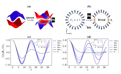
Figure 1: (a) Topological quench dynamics influenced by quantum noise. (b) Quench-induced dynamical topology defined on BIS can be destroyed by sufficiently strong noise. $\boldsymbol{k}_{c}$ (red stars) denotes the singularity momentum on the dBIS, where the spin polarization dynamics lose oscillation behavior ($\overline{\langle\langle\boldsymbol{\sigma}(\mathbf{k})\rangle\rangle}_{r}\neq 0$), leading to ill-defined dBIS and the topological trivial phase. (c) The dynamical spin polarization of $\sigma_{z}$ on $\boldsymbol{k}_{c}$ under weak noise $\lambda=0.2<\lambda_{c}$ ($\lambda_{c}\approx 0.39$ for studied model). (d) The dynamical spin polarization of $\sigma_{z}$ on $\boldsymbol{k}_{c}$ under strong noise $\lambda=0.8>\lambda_{c}$. In (c) and (d), the purple lines depict the results of the clean system, while the grey lines represent the results under Markovian noise. The blue lines labeled NM1, NM2, NM3, NM4 correspond to the results obtained with non-Markovian noise, with non-Markovianity parameter $b=2,1,0.6,0.2$, respectively. The insets in (c) and (d) display the oscillation frequency $\omega$ derived from the corresponding spin polarization dynamics.

Quench-induced topological dynamics.—Quantum quenches provide a nonequilibrium approach to investigating topological physics Vajna and Dóra (2015); Caio et al. (2015); Budich and Heyl (2016); Wilson et al. (2016); Fläschner et al. (2018); Ünal et al. (2020); Hu and Zhao (2020). This has spurred numerous experimental investigations across various quantum simulation platforms, including ultracold atoms Sun et al. (2018); Yi et al. (2019), nuclear magnetic resonance (NMR) Xin et al. (2020), nitrogen-vacancy defects in diamond Ji et al. (2020), and superconducting circuits Niu et al. (2021). Once referring to simulation experiments on quantum devices, environmental noise becomes an inevitable problem. Recently, there has been a surge of interest in exploring the interplay between topology physics and noisy environment, where diverse nonequilibrium topological phenomena emerged Heiss (2012); Lee (2016); Leykam et al. (2017); Xu et al. (2017); Kunst et al. (2018); Yao et al. (2018); Zhang et al. (2021); Lin et al. (2022).

In this Letter, we explore the effect of non-Markovian noise in quench-induced dynamical topology simulation. We consider the 2D quantum anomalous Hall (QAH) model in momentum space,

$$H_{QAH}(\mathbf{k})=\mathbf{h}(\mathbf{k})\cdot\boldsymbol{\sigma},$$ (8)

with Bloch vector $\mathbf{h}(\mathbf{k})=(t_{so}\sin{k_{x}},t_{so}\sin{k_{y}},m_{z}-t_{0}\cos{k_{x}}-t_{0}\cos{k_{y}})$. Here $t_{0}$ and $t_{so}$ are the spin-conserved and spin-flipped hopping coefficients, and $m_{z}$ is the magnetic field. We set the quenched Hamiltonian parameters as $m_{z}=1.2$, $t_{so}=0.2$, and $t_{0}=1$ throughout this work. For $0<|m_{z}|<2|t_{0}|$, $H_{QAH}$ exhibits nontrivial QAH behavior characterized by Chern number $C_{1}=-\text{sgn}\left(m_{z}\right)$.

We focus on the quench dynamics by varying $m_{z}$ suddenly from $m_{z}\gg t_{0}$ trivial phase ($|{\uparrow}\rangle$ for all $\mathbf{k}$) into $0<|m_{z}|<2|t_{0}|$ Chern insulating phase. In this context, we define the dynamical spin polarization and the time-averaged spin polarization as $\langle\langle\boldsymbol{\sigma}(\mathbf{k},t_{n})\rangle\rangle_{r}=\text{Tr}[\rho(\mathbf{k},t_{n})\boldsymbol{\sigma}]$ and $\overline{\langle\langle\boldsymbol{\sigma}(\mathbf{k})\rangle\rangle}_{r}=\lim_{T\rightarrow{\infty}}\frac{1}{T}\int_{0}^{T}dt\ \langle\langle\boldsymbol{\sigma}(\mathbf{k},t)\rangle\rangle_{r}$, respectively. The nontrivial topology emerges on band inversion surface (BIS) Zhang et al. (2018, 2019, 2020, 2022) during the quench dynamics, where BIS is defined as a $\mathbf{k}$-subspace that supports spin-flip resonant oscillations, resulting in the vanishing time-averaged spin polarization $\overline{\langle\langle\boldsymbol{\sigma}(\mathbf{k})\rangle\rangle}_{r}=0$.

Once the QAH model is coupled to the stochastic environment, the Hamiltonian takes the form

$$H(\textbf{k},t)=H_{QAH}(\textbf{k})+\textbf{B}(\textbf{k},t)\cdot\boldsymbol{\sigma},$$ (9)

and the dynamics of the system are governed by the time evolution in Eq. (2). Under Markovian noise Zhang et al. (2021); Lin et al. (2022), the dynamical topology can be preserved on a noise-deformed band inversion surface (dBIS) if the noise strength is confined within a specific range, known as the sweet spot region. However, when the noise strength exceeds this sweet spot region, the bulk gap of the resulting dynamical phase closes. As a consequence, the dynamical oscillation of spin polarization at certain momentum vanishes, leading to an ill-defined dBIS and ultimately resulting in a topologically trivial phase.

We focus on pure dephasing bath defined in Eq. (Non-Markovianity Benefits Quantum Dynamics Simulation). In the Markovian limit, the sweet spot region that respects the dynamical topology is

$$\lambda\leq\lambda_{c}=\min_{\mathbf{k}\in\text{dBISs}}2\|(h_{x}(\mathbf{k}),h_{y}(\mathbf{k}))\|,$$ (10)

where $\lambda$ is the noise strength and $\lambda_{c}\approx 0.39$ in our setup. In terms of non-Markovian pure dephasing noise, the dynamics simulation results are presented in Fig. 1. When weak noise is within the sweet spot region (Fig. 1(c)), the dynamical spin polarization at $\boldsymbol{k}_{c}$ exhibits decay companing with oscillation behavior in the Markovian limit. After rescaling the dynamical process by neglecting the amplitude decay while keeping the oscillation, dBIS can be well defined ($\overline{\langle\langle\boldsymbol{\sigma}(\mathbf{k})\rangle\rangle}_{r}=0$) thereby preserving the dynamical topology. As non-Markovian effects are gradually introduced, the dynamical spin polarization dynamics approaches cleaner cases with weaker amplitude decay, compared to the original Markovian scenario.

For strong noise strength outside the sweet spot region in the Markovian limit (Fig. 1(d)), the dynamical spin polarization at $\boldsymbol{k}_{c}$ exhibits serious decay without oscillation behavior (oscillation frequency is $\omega=0$ given by Fourier transformation). Consequently, the dBIS becomes ill-defined, resulting in a noise induced topologically trivial phase. Once the non-Markovanity is turned on gradually, the dynamical spin polarization displays behavior similar to the weak noise case, with a finite oscillation frequency similar to the noiseless value. This leads to the successful recovery of a well-defined dBIS and the restoration of the topology from the detrimental effects of strong noise, i.e. non-Markovianity induced topological phase recovery. (See more numerical results in the SM). These results collectively demonstrate that the non-Markovianity presented in quantum noise benefits the dynamics simulation process and drives a topological phase recovering from a trivial one under strong noise.

Many-body localization dynamics.—Many-body localization (MBL) is one of the cornerstones of non-equilibrium physics which brings a robust exception of eigenstate thermalization hypothesis Srednicki (1994). Starting from Anderson localization Anderson (1958b), the system can avoid thermalization with many-body interactions turned on Basko et al. (2006) due to the emergence of local integrals of motion Serbyn et al. (2013a). Strong random disorder Oganesyan and Huse (2007); Pal and Huse (2010); Nandkishore and Huse (2015); Altman and Vosk (2015); Abanin et al. (2019), quasiperiodic potential Iyer et al. (2013); Khemani et al. (2017); Zhang and Yao (2018, 2019); Kohlert et al. (2019) and linear potential Schulz et al. (2019); van Nieuwenburg et al. (2019); Khemani et al. (2020); Doggen et al. (2021); Liu et al. (2023a) can all lead to many-body localization in one dimension. As one of the most important non-equilibrium quantum phases as well as the foundation for other novel phases such as discrete time crystal Else et al. (2020); Zaletel et al. (2023) and Hilbert space fragmentation Khemani et al. (2020); Doggen et al. (2021); Yang et al. (2020), MBL system has been extensively explored on different experimental platforms of programmable quantum simulators and quantum computers Schreiber et al. (2015); Smith et al. (2016); Liu et al. (2023b); Gong et al. (2021). Therefore, a comprehensive investigation of the quantum noise effect for MBL simulation is highly desired. The decoherence effect on the MBL system has been investigated in Ref. Levi et al. (2016), where only Markovian dephasing noise is considered.

In this Letter, we investigate the interplay between quantum decoherence with and without non-Markovianity and the one-dimensional spin model hosting MBL with on-site quenched disorder. The MBL Hamiltonian with open boundary conditions reads:

$$H_{\text{MBL}}=\sum_{i}\left(S^{x}_{i}S^{x}_{i+1}+S^{y}_{i}S^{y}_{i+1}+J_{z}S^{z}_{i}S^{z}_{i+1}\right)+\sum_{i}W_{i}S^{z}_{i}.$$ (11)

The interaction term $J_{z}=0.2$, and $W_{i}$ is the static-random fields sampled from a Gaussian distribution $N(0,W/\sqrt{3})$, where we use $W=10$ deeply in the MBL phases. Note that the random variable is so chosen that it can be directly comparable with the form of dephasing noise (see the SM for details). The phase diagram for this clean model can also be found in the SM.

We employ two representative observables: charge imbalance and entanglement entropy to probe the characteristics of MBL dynamics. Charge imbalance $\mathcal{I}$ is defined as the difference in occupation numbers between odd and even sites $\mathcal{I}=\sum_{i}(-)^{i}\langle S^{z}_{i}\rangle$, assuming that the initial state is an antiferromagnetic product state. It is expected to be (non-)zero for thermal (MBL) phases at infinite time limit with exponential decay at later times in thermal phases. The half-chain entanglement entropy $S$, defined as the von Neumann entropy of the reduced density matrix on half of the system, provides a more intrinsic information perspective of MBL phases, exhibiting a logarithmic increase before saturating to a non-thermal value Bardarson et al. (2012); Serbyn et al. (2013b). In systems of very weak thermalization, e.g. MBL systems coupled to weak Markovian dephasing Levi et al. (2016); Wybo et al. (2020), entanglement can still follow the logarithmic scaling but with saturating value $S(t\rightarrow\infty)$ the same as the typical thermal value.

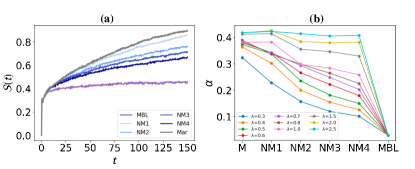
Figure 2: (a) Entanglement entropy of many-body localization dynamics with pure dephasing noise of strength $\lambda=0.4$. The purple line shows the results of the clean MBL system. The grey line shows the results under Markovian noise. Blue lines labeled from NM1 to NM4 show the results under non-Markovian noise with non-Markovianity parameter $b=4,1,0.5,0.2$. (b) Parameter $\alpha$ that fits the late-time entanglement entropy dynamics in scaling relation $S(t)\sim\alpha\log(t+\gamma)+\beta$ under Markovian bath (M), non-Markovian bath (NM1-NM4) and original MBL with varying noise strength $\lambda$.

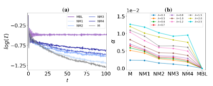
Figure 3: (a) Charge imbalance of many-body localization dynamics with pure dephasing noise of strength $\lambda=0.7$. The purple line shows the results of the clean MBL system. The grey line shows the results under Markovian noise. Blue lines labeled from NM1 to NM4 show the results under non-Markovian noise with non-Markovianity parameter $b=4,1,0.5,0.2$. (b) Parameter $\alpha$ that fits the late-time charge imbalance dynamics in scaling relation $\mathcal{I}(t)\sim e^{-\alpha t+\beta}$ under Markovian noise (M), non-Markovian noise (NM1-NM4) and clean MBL with varying noise strength $\lambda$.

To compute the entanglement entropy in the context of Monte Carlo trajectory simulation for the quantum noise environment, we compute the trajectory averaged entanglement entropy but not the reverse (entropy on trajectory averaged density matrix). The conceptual subtlety here is from the non-linearity of the definition of entropy Skinner et al. (2019); Chan et al. (2019); Li et al. (2018). In view of trajectory level dynamics, MBL dynamics with single noise realization introduce temporal randomness apart from the spatial randomness presented in pure MBL system. The difference is similar to the Floquet circuit/random circuit or static Hamiltonian/Brownian Hamiltonian Lashkari et al. (2013); Sahu and Jian (2023) scenarios. In our setup, dephasing noises with and without non-Markovianity enter the external field $W_{i}$ term in the Hamiltonian Eq. (11). The Markovian quantum noise is independent at each time slice and thus is of Brownian type. On the contrary, non-Markovian noise has a temporal correlation between different times and goes beyond the Brownian paradigm.

With the introduction of quantum noise in the time evolution, i.e. with the coupling to the environment, the system under investigation will eventually be thermal. One interesting question that arises is whether the non-Markovianity in quantum noise can lead to slower thermalization and preserve the many-body localization characteristics to some extent in the simulation. We numerically study the MBL dynamics simulation of $N=8$ qubit system with (non-)Markovian quantum noise of different strengths and different non-Markovianity degrees. The results for entanglement entropy and charge imbalance are illustrated in Fig. 2 and Fig. 3, respectively. The left panel of both figures shows the dynamics of a given noise strength $\lambda$ with varying non-Markovianity. In the right panel, we fit the later time dynamics to extract the relevant scaling quantities reflecting the speed of thermalization. For late-time dynamics, we use the scaling relation $\alpha\log(t+\gamma)+\beta$ and $e^{-\alpha t+\beta}$ to fit these two quantities. In both cases, a larger positive $\alpha$ reflects a quicker thermalization. The results in panel (b) of both figures demonstrate that larger noise strength $\lambda$ can lead to stronger thermalization. More interestingly, given the same strength of the quantum noise, the stronger non-Markovianity can lead to a weaker thermalization, indicating a better reflection of the clean MBL dynamics. In other words, the memory effect rooted in non-Markovianity makes it harder to erase the initial state information, which is a signal against thermalization.

Conclusion.— In this Letter, we have investigated the impact of non-Markovian quantum noise on quantum dynamics simulations using both analytical and numerical approaches Zhang et al. (2023). Remarkably, our findings indicate that non-Markovianity can have a beneficial effect by offering enhanced protection for clean dynamics compared to noise of equivalent strength in the Markovian limit. This unexpected conclusion highlights the potential advantages of incorporating non-Markovian noise in quantum simulations. By better preserving the integrity of the system’s dynamics, non-Markovianity offers a promising avenue for improving the accuracy and reliability of quantum simulations across diverse quantum platforms.

Supplemental Materials
Non-Markovianity Benefits Quantum Dynamics Simulation

S1 Time-nonlocal Quantum Master Equation

In this section, we briefly introduce the time-nonlocal master equation that describes general open quantum systems in terms of both quantum environment and classical stochastic noise.

Once a time-independent system $H_{s}$ couples to stochastic baths, the Hamiltonian can be described as

$$H(t)=H_{s}+H_{sb}=H_{s}+\sum_{i}\textbf{B}_{i}(t)\cdot\boldsymbol{\sigma}_{i},$$ (S1)

where $H_{s}$ is the time-independent system Hamiltonian. For quantum noise, $B_{i}^{\alpha}(t)=e^{-iH_{b}t}B_{i}^{\alpha}(0)e^{iH_{b}t}$ is a bath operator in the interaction picture with respect to $H_{b}$ – the environment Hamiltonian. Index $\alpha$ is one of the ${x,y,z}$ Cartesian components and index $i$ labels the freedoms of qubits. For classical stochastic baths, the system is not explicitly coupled to another quantum system but is subjected to classical noise sources, i.e., $B_{i}^{\alpha}(t)$ is made up of real-valued stochastic processes.

The dynamical process of general open quantum systems is described by the time-nonlocal quantum master equation (TNQME) Breuer and Petruccione (2002):

$$\frac{d\rho(t)}{dt}=\mathcal{L}_{s}\rho(t)+\int_{0}^{t}dt^{\prime}\mathcal{K}(t-t^{\prime})\rho(t^{\prime}),$$ (S2)

where $\rho(t)$ denotes the system’s reduced density matrix, $\mathcal{L}_{s}$ is the Liouville superoperator corresponding to the system Hamiltonian, and $\mathcal{K}(t)$ is a memory kernel that fully encodes environment-induced decoherence effects and the memory effect of the evolution history from non-Markovian effect. In terms of the Markovian approximation, the memory kernel is local in time $K(t-t^{\prime})\propto\delta(t-t^{\prime})$ and the master equation is reduced into the Lindblad form. It is also reported that Chen et al. (2020), under the proper definition, dynamics induced by classical stochastic noise can be described by a formally identical time-nonlocal master equation as the quantum one in Eq. (S2).

We consider the Gaussian noise, which can be fully characterized by the first two statistical moments $\langle B_{i}^{\alpha}(t)\rangle$ and a two-time correlation function:

$$C_{\alpha\alpha^{\prime}}(t)=\langle B^{\alpha}(t)B^{\alpha^{\prime}}(0)\rangle.$$ (S3)

For Gaussian noise, the memory kernel $\mathcal{K}(t)=\sum_{n=1}^{\infty}\mathcal{K}_{2n}(t)$, where $K_{2n}(t)$ denotes order-$2n$ expansion of the Hamiltonian with respect to $H_{sb}$. The memory kernel is directly related to time correlation function of the noise profile. For example, the leading order of memory kernel in a weak noise regime gives

$$\mathcal{K}(t)(\cdot)\approx\sum_{\alpha,\alpha^{\prime}}[\sigma^{\alpha},C_{\alpha\alpha^{\prime}}(t)\sigma^{\alpha^{\prime}}(t)(\cdot)-C_{\alpha\alpha^{\prime}}^{*}(t)(\cdot)\sigma^{\alpha^{\prime}}(t)],$$ (S4)

where $\sigma^{\alpha}(t)=e^{-iH_{s}t}\sigma^{\alpha}e^{iH_{s}t}$ and $C_{\alpha\alpha^{\prime}}(t)$ is the time correlation function defined in Eq. (S3). Namely, we can replace the quantum bath with classical stochastic noise with the identical correlation matrix and obtain the same noisy dynamics. This equivalence underlines the Monte Carlo trajectory noisy dynamics numerical simulation of this work. The noise spectral density is defined for real valued correlation matrix via Fourier transformation as

$$S_{\alpha\alpha^{\prime}}(\omega)=\int_{-\infty}^{\infty}dte^{i\omega t}C_{\alpha\alpha^{\prime}}(t).$$ (S5)

If the correlation function for the environment noise decays significantly faster than the characteristic time scale of the system’s evolution, the temporal correlation function can be treated as a delta function with a uniform spectral density. The correlation time and the memory effect in this Markovian limit are regarded to be zero. Therefore, Markovian noise is only a special limit of the general non-Markovian noise.

S2 Non-Markovian Pure-dephasing Noise

In this section, we present the theory framework of non-Markovian pure-dephasing noise and analytically analyze corresponding dynamical behavior induced by non-Markovianity for idle qubits.

In general, decoherence coming from the environment is a complicated process involving both population relaxation and dephasing. However, when we enhance the intensity of an external polarization field to a point where the energy level separations are significantly large, the relaxation process can be rendered insignificant within the relevant timeframe, leaving dephasing as the sole main cause of decoherence. In the context of this pure dephasing assumption, the environmental noise can be represented as random fields that induce random phase shifts. This approach is applicable in various dephasing environments, such as spin baths in solid-state systems Biercuk et al. (2009); De Lange et al. (2010); Ajoy et al. (2011) and background noise in superconducting qubits Cywiński et al. (2008). The pure dephasing Hamiltonian of $N$-qubit open systems reads

$$H_{sb}=\sum_{i=1}^{N}B_{i}^{z}(t)\sigma_{z_{i}},$$ (S6)

where we assume the Gaussian noise with $\langle\langle B_{i}^{z}(t)\rangle\rangle_{r}=0$ and time correlation function $C(t-t^{\prime})=\langle\langle B_{i}^{z}(t)B_{j}^{z}(t^{\prime})\rangle\rangle_{r}\delta_{i,j}$. $\delta_{i,j}$ denotes that the noise experienced by each qubit is independent of each other. The temporal correlation function of $B_{i}(t)$ with finite correlation length can be recognized as the instigator of the non-Markovian memory effect, see Sec. S1.

Considering a general initial pure state $|\psi(0)\rangle=\sum_{\vec{s}=00\cdots 0}^{11\cdots 1}\alpha_{\vec{s}}|\vec{s}\rangle$, $\vec{s}=s_{1}s_{2}\cdots s_{N}$, $s_{i}=0$ or $1$, the quantum state at time $t$ under pure dephasing bath becomes

$$\bar{\rho}_{\vec{s},\vec{s}^{\prime}}(t)=\alpha_{\vec{s}}\alpha_{\vec{s}^{\prime}}^{*}\langle\langle e^{-2i\sum_{l=1}^{N}(s^{\prime}_{l}-s_{l})F_{l}(t)}\rangle\rangle_{r}$$ (S7)

where $F_{l}(t)\equiv\int_{0}^{t}B_{l}(\tau)d\tau$ and $\langle\langle\cdots\rangle\rangle_{r}$ denotes average over noise configurations. For initially uncorrelated qubits and environments, the open system state $\rho(0)$ is linearly mapped to the corresponding state at time $t$ by dynamical maps $\Lambda(t)$

$$\rho(t)=\Lambda(t)\rho(0)$$ (S8)

Dynamical maps $\Lambda$ are superoperators (of dimension $d^{2}\times d^{2}$, $d=2^{N}$) and the map is carried out as a matrix-vector product when the density matrix $\rho$ is vectorized as length $d^{2}$. The structure form of $\Lambda$ brings many operational advantages. For instance, a succession of transitions can be performed with simple matrix multiplications, eg., $\Lambda_{1}\Lambda_{2}\rho$. For stochastic noise that is independent between qubits, we can focus on single-qubit dynamical maps, and the multiple-qubit dynamical maps can be regarded as tensor products of single-qubit ones. More complicated decoherence coming from correlated noise, i.e., $\langle\langle B^{z}_{i}(t)B^{z}_{j}(t^{\prime})\rangle\rangle_{r}\neq 0$ for $i\neq j$ was presented in Ref. Chen et al. (2020). The single-qubit dynamics in terms of density matrix elements reads

$$\bar{\rho}_{0,1}(t) = \alpha_{0}\alpha_{1}^{*}\langle\langle e^{-2iF(t)}\rangle\rangle_{r}=\bar{\rho}_{0,1}(0)e^{-2\langle\langle F(t)^{2}\rangle\rangle_{r}}=\bar{\rho}_{0,1}(0)e^{-\Gamma(t)},$$ (S9)

$$\bar{\rho}_{1,0}(t) = \alpha_{0}^{*}\alpha_{1}\langle\langle e^{-2iF(t)}\rangle\rangle_{r}=\bar{\rho}_{1,0}(0)e^{-2\langle\langle F(t)^{2}\rangle\rangle_{r}}=\bar{\rho}_{1,0}(0)e^{-\Gamma(t)},$$

$$\bar{\rho}_{0,0}(t) = \bar{\rho}_{0,0}(0),\ \bar{\rho}_{1,1}(t)=\bar{\rho}_{1,1}(0),$$

where the decoherence rate $\Gamma(t)$ can be obtained from time correlation function

$$\Gamma(t) = 2\langle\langle F(t)^{2}\rangle\rangle_{n}$$

$$= 2\int_{0}^{t}\int_{0}^{t}\langle\langle B^{z}(t^{\prime})B^{z}(t^{\prime\prime})\rangle\rangle_{n}dt^{\prime}dt^{\prime\prime}$$

$$= 2\int_{0}^{t}\int_{0}^{t}C(t^{\prime}-t^{\prime\prime})dt^{\prime}dt^{\prime\prime}$$

The noise spectral density $S(\omega)$ provides the energy distribution of the noise signal at different frequencies and often be used as the most important characteristic of noise sources. In this work, we assume the reservoir has a Lorentzian spectrum Imamog et al. (1994); Park et al. (2000),

$$S(\omega)=\frac{\lambda b}{b^{2}+(\omega-\omega_{c})^{2}}.$$ (S11)

According to Sec. S1, the corresponding time correlation function becomes

$$C(t-t^{\prime})=\lambda e^{-b|t-t^{\prime}|}\cos{[\omega_{c}(t-t^{\prime})]}.$$ (S12)

Based on Eq. S9 and Eq. S2, we can analytically obtain the pure-dephasing dynamical maps,

$$\Lambda(t)=\begin{bmatrix}1&0&0&0\\ 0&e^{-\Gamma(t)}&0&0\\ 0&0&e^{-\Gamma(t)}&0\\ 0&0&0&1\\ \end{bmatrix},$$ (S13)

with

$$\Gamma(t)=\frac{4}{\pi}\int_{0}^{\infty}d\omega\frac{S(\omega)}{\omega^{2}}[1-\cos{(\omega t)}].$$ (S14)

It is straightforward to verify that these maps are in general not divisible, i.e.,$\Lambda_{n+m}\neq\Lambda_{n}\Lambda_{m}$. We note that those analytical results benefiting our understanding are owing to the pure dephasing case in which all terms in $H_{sb}$ commute with each other. Otherwise, the dynamical maps and non-Markovianity have to be obtained by various quantum tomography methods Chen et al. (2020, 2022).

We denote $C(0)=\lambda$ in Eq. (S12) as the noise strength parameter, which can be directly interpolated to the noise strength defined in the usual Markovian bath. For instance, for white noise sampled from Gaussian distribution $N(0,\sqrt{\lambda})$, the correlation function exhibits $C(t)=\lambda\delta(t)$ with noise strength $\lambda$. Additionally, $b$ in Eq. (S12) characterizes the non-Markovianity, which governs the correlation time scale for the noise profile. With smaller $b$, the correlation length is larger, indicating stronger non-Markovianity. We discuss cases with different values of $b$:

1) Markovian limit $b\rightarrow\infty$,

$$|C(t-t^{\prime})|=\lambda\cdot\delta(t-t^{\prime}).$$ (S15)

For pure dephasing in Eq. (S13), $\Gamma(t)=2\lambda t$, the dynamical map satisfies $\Lambda_{n+m}=\Lambda_{n}\Lambda_{m}$, and is thus Markovian.

2)Dynamical noise processes with finite $b$ lead to moderate non-Markovianity.

According to Sec. S1, we qualitatively realize that the temporal correlation function of $B_{i}(t)$ with finite correlation time can be recognized as the instigator of the non-Markovian memory effect. We further involve transfer tensor to quantitatively represent the relationship between correlation function and non-Markovianity. Dynamical evolution up to time $t_{n}$ depends on the system’s history through multiple transfer tensors indicating a memory effect

$$\rho(t_{n})=\sum_{m=1}^{K}T_{m}\rho(t_{n-m}),\ \$$ (S16)

which offers a simple discretized way to characterize non-Markovian evolution since $T_{n}\approx\mathcal{K}(t_{n})\delta t^{2}$. More effective transfer tensor maps (larger $K$, $\|T_{i}\|\geq\epsilon,i\in[1,K]$) denote stronger non-Markovianity and longer history memory. We show it explicitly with transfer tensor maps stated in the main text in Fig. S1. As we can see, smaller $b$ corresponds to a longer correlation length in Fig. S1(a) and stronger non-Markovianity (longer memory on the history dynamics) in Fig. S1(b).

Starting from an initial state $|\psi(0)\rangle=|0\rangle+|1\rangle$, according to Eq. (S13), the instantaneous state can be derived, see Fig. S1(c)(d). It is obvious that the decoherence of the initial state is weaker under smaller noise strength $\lambda$ with the same $b$ and under stronger non-Markovianity (smaller $b$) with the same $\lambda$.

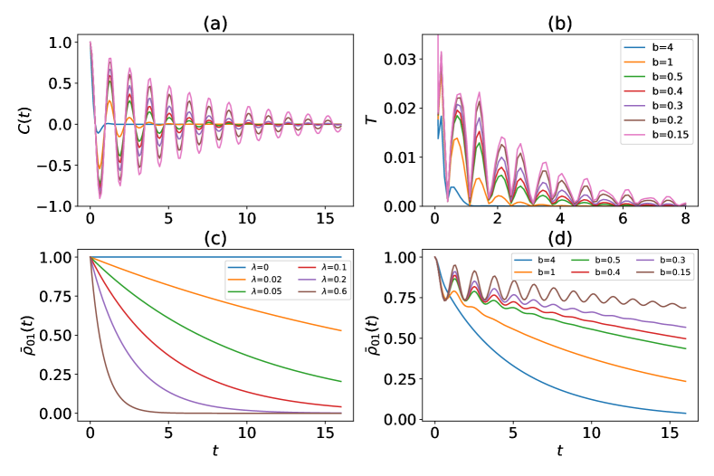
Figure S1: Non-Markovian pure dephasing noise in Lorentzian form. (a) The real part of correlation functions changes along with time with $\lambda=1$. (b) The transfer tensor maps in 2-norm change along with time distance $t=\delta t\,n$ ($\delta t=0.2$). (c) The relaxation dynamics of the idle qubit under varying noise strength $\lambda$ with $b=1$. (d) The relaxation dynamics of the idle qubit under varying non-Markovianity $b$ with $\lambda=1$. We set $\omega_{c}=5$.

S3 Stochastic Simulation of non-Markovian Processes

In the former section, we analytically analyze the dynamical maps and non-Markovian behavior focusing on the pure dephasing noise bath alone ($H_{s}=0$). Once we want to simulate interesting quantum systems $H_{s}$ in a general non-Markovian reservoir, i.e.,$H=H_{s}+H_{sb}$, the quantitative consequence is hard to track analytically even in the non-Markovian pure dephasing noise case. Instead, we simulate the dynamics by stochastic processes in discretized time steps, in which the stochastic noise is generated using the Fast Fourier Transform (FFT) method Heideman et al. (1985). The average results over different stochastic processes are equivalent to the dynamics of the given system with non-Markovian noise.

This numerical method uses the relation of the correlation function $C(t)$ to the non-negative real-valued spectral density $S(\omega)$. The integral can be approximated by a discrete integration scheme

$$C(t)=\int_{-\infty}^{\infty}\mathrm{d}\omega\,\frac{S(\omega)}{\pi}e^{-\mathrm{i}\omega t}\approx\sum_{k=0}^{N-1}\Delta\omega\frac{S(\omega_{k})}{\pi}e^{-\mathrm{i}\omega_{k}t}.$$ (S17)

where $\omega_{k}=\omega_{min}+k\Delta\omega$, $\Delta\omega=(\omega_{max}-\omega_{min})/(N-1)$, $t_{n}=n\delta t$ and $N\Delta\omega\delta t=2\pi$. $N,\omega_{min},\omega_{max}$ are hyperparameters set to satisfy the required tolerance from the following approximations.

For a stochastic process defined as

$$f(t)=\sum_{k=0}^{N-1}\sqrt{\frac{\Delta\omega S(\omega_{k})}{\pi}}Y_{k}e^{-\mathrm{i}\omega_{k}t},$$ (S18)

with independent complex random variables $Y_{k}$ such that $\langle Y_{k}\rangle=0$ and $\langle Y_{k}Y^{\ast}_{k^{\prime}}\rangle=\delta_{k,k^{\prime}}$, it is easy to identify that its correlation function will be the same as the expected correlation function from non-Markovian dephasing noise,

$$\langle f(t)f^{\ast}(t^{\prime})\rangle = \sum_{k,k^{\prime}}\frac{1}{\pi}\sqrt{\Delta\omega^{2}S(\omega_{k})S(\omega_{k^{\prime}})}\langle Y_{k}Y^{\ast}_{k^{\prime}}\rangle\exp[-\mathrm{i}(\omega_{k}t-\omega_{k^{\prime}}t^{\prime})]$$

$$= \sum_{k}\frac{\Delta\omega}{\pi}S(\omega_{k})e^{-\mathrm{i}\omega_{k}(t-t^{\prime})}$$

$$\approx C(t-t^{\prime}).$$

The discrete-time stochastic process of $f(t)$ in the time domain can be realized by

$$f(t_{n})=e^{-\mathrm{i}\omega_{\mathrm{min}}t_{n}}\mathrm{FFT}\left(\sqrt{\frac{\Delta\omega S(\omega_{k})}{\pi}}Y_{k}\right),$$ (S20)

where $Y_{k}$ are Gaussian distributed random variables. It is easy to see that, the discrete-time stochastic process generated above can support noise in different random field directions and even noise correlation between qubits, i.e., $B^{\alpha}(t),\alpha=x,y,z$ or $\langle B_{i}B_{j}\rangle_{i\neq j}\neq 0$ beyond the qubit-independent pure dephasing model in Sec. S2.

S4 Non-Markovianity in quench-induced Dynamical Topology Simulation

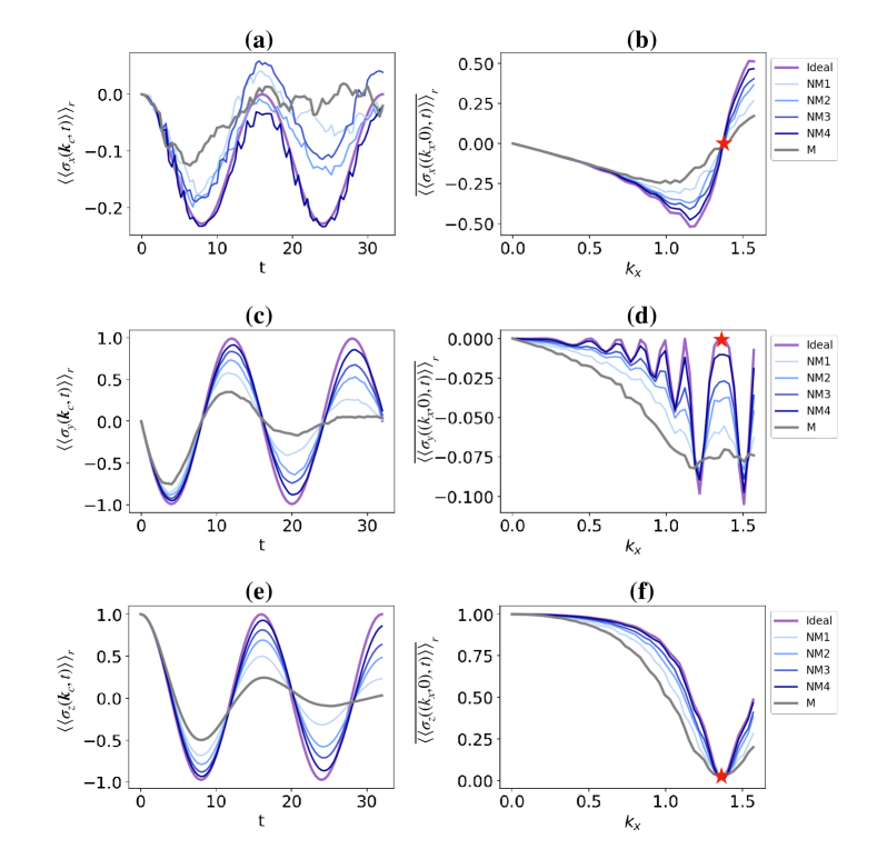
Figure S2: Dynamical spin polarization and time-averaged spin polarization. Under weak noise strength $\lambda=0.2<\lambda_{c}$ ( $\lambda_{c}\approx 0.39$ for the studied model): The dynamical spin polarization (a)$\langle\langle\sigma_{x}\rangle\rangle_{r}$, (c) $\langle\langle\sigma_{y}\rangle\rangle_{r}$, (e) $\langle\langle\sigma_{z}\rangle\rangle_{r}$ on dBIS at $\boldsymbol{k}_{c}$. $\boldsymbol{k}_{c}$ (red stars) denotes the singularity momentum (defined in the main text or the right plane of this figure), the spin polarization dynamics first lose oscillation on the dBIS at $\boldsymbol{k}_{c}$ with the increase of noise leading to ill-defined dBIS and topological trivial phases. The time averaged spin polarization (b) $\overline{\langle\langle\sigma_{x}\rangle\rangle}_{r}$, (d) $\overline{\langle\langle\sigma_{y}\rangle\rangle_{r}}$, (f) $\overline{\langle\langle\sigma_{z}\rangle\rangle_{r}}$ at the momentum line $k_{y}=0$. The purple lines (Ideal) show the results of a clean system. The grey lines (M) show the results under Markovian noise. The blue lines from lightest to heaviest (NM1,NM2,NM3,NM4) show the results of non-Markovian noise with non-Markovianity parameterc $b=2,1,0.6,0.2$. The system parameters are chosen as $m_{z}=1.2,t_{so}=0.2,t_{0}=1$.

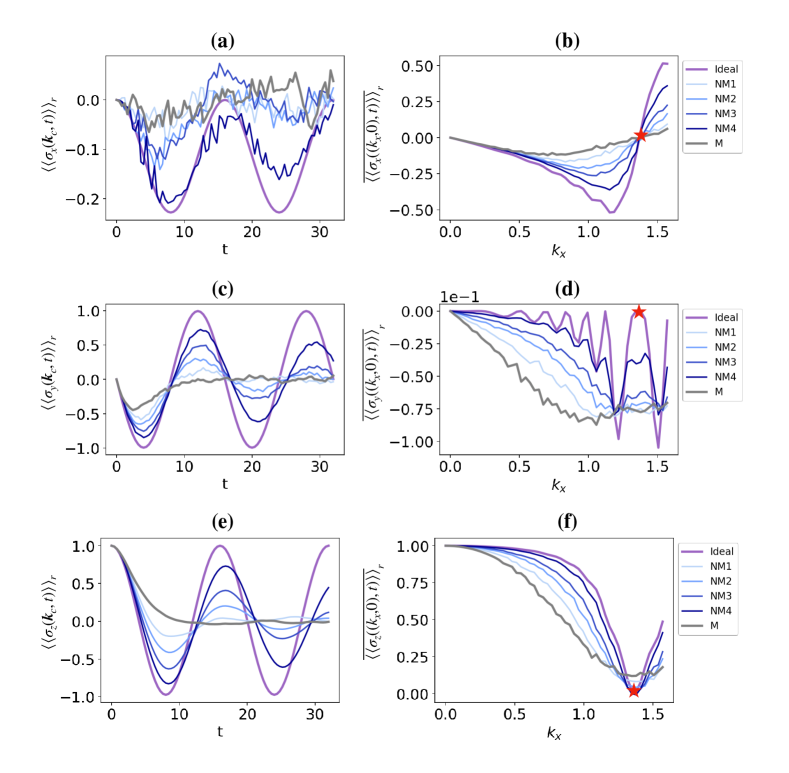
Figure S3: Dynamical spin polarization and time-averaged spin polarization. Under strong noise strength $\lambda=0.8>\lambda_{c}$: The dynamical spin polarization (a)$\langle\langle\sigma_{x}\rangle\rangle_{r}$, (c) $\langle\langle\sigma_{y}\rangle\rangle_{r}$, (e) $\langle\langle\sigma_{z}\rangle\rangle_{r}$ on dBIS at $\boldsymbol{k}_{c}$. $\boldsymbol{k}_{c}$ (red stars) denotes the singularity momentum (defined in the main text or the right plane of this figure), the spin polarization dynamics first lose oscillation on the dBIS at $\boldsymbol{k}_{c}$ with the increase of noise leading to ill-defined dBIS and topological trivial phases. The time averaged spin polarization (b) $\overline{\langle\langle\sigma_{x}\rangle\rangle}_{r}$, (d) $\overline{\langle\langle\sigma_{y}\rangle\rangle_{r}}$, (f) $\overline{\langle\langle\sigma_{z}\rangle\rangle_{r}}$ at the momentum $k_{y}=0$. The purple lines (Ideal) show the results of a clean system. The grey lines (M) show the results under Markovian noise. The blue lines from lightest to heaviest (NM1,NM2,NM3,NM4) show the results of non-Markovian noise with non-Markovianity parameter $b=2,1,0.6,0.2$. The system parameters are chosen as $m_{z}=1.2,t_{so}=0.2,t_{0}=1$.

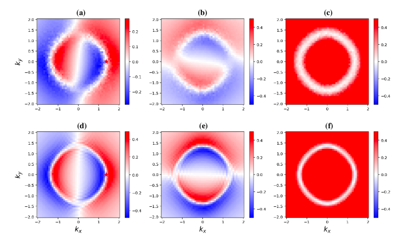
Figure S4: Time-averaged spin polarization under weak noise $\lambda=0.2$ in the Markovian limit: (a) $\overline{\langle\langle\sigma_{x}\rangle\rangle_{r}}$, (b) $\overline{\langle\langle\sigma_{y}\rangle\rangle_{r}}$, (c) $\overline{\langle\langle\sigma_{z}\rangle\rangle_{r}}$. Time-averaged spin polarization under weak noise $\lambda=0.2$ with non-Markovianity parameter $b=0.2$: (d) $\overline{\langle\langle\sigma_{x}\rangle\rangle_{r}}$, (e) $\overline{\langle\langle\sigma_{y}\rangle\rangle_{r}}$, (f) $\overline{\langle\langle\sigma_{z}\rangle\rangle_{r}}$.

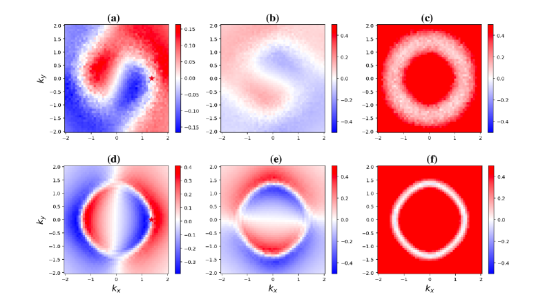
Figure S5: Time-averaged spin polarization under strong noise $\lambda=0.8$ in the Markovian limit: (a) $\overline{\langle\langle\sigma_{x}\rangle\rangle}_{r}$, (b) $\overline{\langle\langle\sigma_{y}\rangle\rangle}_{r}$, (c) $\overline{\langle\langle\sigma_{z}\rangle\rangle}_{r}$. Time-averaged spin polarization under strong noise $\lambda=0.8$ with non-Markovianity parameter $b=0.2$: (d) $\overline{\langle\langle\sigma_{x}\rangle\rangle}_{r}$, (e) $\overline{\langle\langle\sigma_{y}\rangle\rangle}_{r}$, (f) $\overline{\langle\langle\sigma_{z}\rangle\rangle}_{r}$.

In this section, we summarize the theory of quench-induced dynamical topology of the 2D quantum anomalous Hall (QAH) mode with Markovian noise and present the simulation details and results with the influence from non-Markovianity.

Extensive studies have been carried out in recent years on topological quantum matter Hasan and Kane (2010); Qi and Zhang (2011); Chiu et al. (2016); Sato and Ando (2017), surpassing the established Landau-Ginzburg-Wilson framework Landau and Lifshitz (1999). Notably, researchers have discovered that topological phases, originally defined in the ground state under equilibrium conditions, can also be explored using quantum quenches, which provide a nonequilibrium approach to studying topological physics Vajna and Dóra (2015); Caio et al. (2015); Budich and Heyl (2016); Wilson et al. (2016); Fläschner et al. (2018); Ünal et al. (2020); Hu and Zhao (2020). In this context, the concept of the dynamical bulk-surface correspondence has been introduced as a momentum-space counterpart to the bulk-boundary correspondence. This correspondence establishes a connection between the bulk topology of an equilibrium phase and the emergence of a nontrivial dynamical topological phase on specific momentum subspaces known as band-inversion surfaces (BISs) when the system undergoes a quench across topological transitions Zhang et al. (2018, 2019, 2020, 2022). This dynamical topology offers a versatile method for characterizing and detecting topological phases through quantum dynamics, leading to numerous experimental studies in various quantum simulation platforms, including ultracold atoms Sun et al. (2018); Yi et al. (2019), nuclear magnetic resonance (NMR), nitrogen-vacancy defects in diamond Ji et al. (2020); Xin et al. (2020), and superconducting circuits Niu et al. (2021). Once it comes to simulation experiments on quantum platforms, environmental noise becomes an inevitable problem. Recently, there has been a surge of interest in exploring the interplay between system topology and noise environment, where the influence has led to the emergence of diverse dynamical topological phenomena Heiss (2012); Lee (2016); Leykam et al. (2017); Xu et al. (2017); Kunst et al. (2018); Yao et al. (2018); Zhang et al. (2021); Lin et al. (2022).

According to ref. Zhang et al. (2021), the stochastic Markovian noise with $\langle\langle B^{\alpha}(t)\rangle\rangle_{r}=0$ and $\langle\langle B^{\alpha}(t)B^{\beta}(t^{\prime})\rangle\rangle_{r}=\lambda_{\alpha}\delta(t-t^{\prime})\delta_{\alpha,\beta}$ make the quantum dynamics of the QAH system follow the master equation

$$\frac{d\rho(t)}{dt}=-i[H_{QAH},\rho(t)]+\sum_{\alpha=x,y,z}B_{\alpha}[\sigma_{\alpha}\rho(t)\sigma_{\alpha}-\rho(t)].$$ (S21)

The dynamical spin polarization is defined by $\mathbf{s}(\boldsymbol{k},t)\equiv\langle\langle\boldsymbol{\sigma}(\mathbf{k},t)\rangle\rangle_{r}=\text{Tr}[\rho(\mathbf{k},t)\boldsymbol{\sigma}]$, $\rho(\mathbf{k},t)$ is the density matrix which can be expressed as $\rho(\mathbf{k},t)=1/2[1+\mathbf{s}(\mathbf{k},t)\cdot\boldsymbol{\sigma}]$ for the two band model. The dynamical evolution of spin polarization is governed by Liouvillian superoperator as $\partial_{t}\mathbf{s}(\mathbf{k},t)=\mathcal{L}(\mathbf{k})\mathbf{s}(\mathbf{k},t)$. For the two-band model, the Liouvillian superoperator can be recast into the following matrix $\mathcal{L}(\mathbf{k})$

$$\mathcal{L}(\mathbf{k})=2\begin{bmatrix}-B^{y}-B^{z}&-h_{z}(\mathbf{k})&h_{y}(\mathbf{k})\\ h_{z}(\mathbf{k})&-B^{x}-B^{z}&-h_{x}(\mathbf{k})\\ -h_{y}(\mathbf{k})&h_{x}(\mathbf{k})&-B^{x}-B^{y}\\ \end{bmatrix}.$$ (S22)

By diagonalizing the Liouvillian superoperator, the dynamical spin polarization can be explicitly acquired

$$\mathbf{s}(\mathbf{k},t)=\mathbf{s_{0}}(\mathbf{k})e^{-\gamma_{0}(\mathbf{k})t}+\mathbf{s_{+}}(\mathbf{k})e^{-[\gamma_{1}(\mathbf{k})+i\omega(\mathbf{k})]t}+\mathbf{s_{-}}(\mathbf{k})e^{-[\gamma_{1}(\mathbf{k})-i\omega(\mathbf{k})]t},$$ (S23)

where the coefficients $\mathbf{s}_{i}(\mathbf{k})=(\mathbf{s}_{i}^{L}(\mathbf{k})\cdot\mathbf{s}(\mathbf{k},0))\mathbf{s}_{i}^{R}(\mathbf{k})$ for $i=0,\pm$. Here $\mathbf{s}_{i}^{L(R)}$ are the left(right) eigenvectors of the Liouvillian superoperator

$$\mathcal{L}^{T}(\mathbf{k})\mathbf{s}_{i}^{L}=-\gamma_{i}\mathbf{s}_{i}^{L},\ \mathcal{L}(\mathbf{k})\mathbf{s}_{i}^{R}=-\gamma_{i}\mathbf{s}_{i}^{R},$$ (S24)

with eigenvalues $\gamma_{0}$ and $\gamma_{\pm}=\gamma_{1}\pm i\omega$ respectively. $\omega$ denotes the oscillation frequency of the dynamical spin polarization. $\gamma_{0,1}$ explicitly reflects the spin dynamics dissipation due to the noise.

The original noiseless dynamical topology is defined on BIS, which denotes a momentum subspace $\{\mathbf{k}|h_{z}(\mathbf{k})=0\}$ with $\mathbf{h}(\mathbf{k})\cdot\mathbf{s}(\mathbf{k},0)=0$, where the spin-flip resonant oscillations occur and thus the time-averaged spin-polarization vanishes: $\lim_{T\rightarrow{\infty}}\int_{0}^{T}dt\ \mathbf{s}(\mathbf{k},t)|_{\mathbf{k}\in BIS}=0$. The noise deformed BIS(dBIS) under noise can also be well defined

$$\text{dBIS}\equiv\{\mathbf{k}|\mathbf{s}_{0}^{L}\cdot\mathbf{s}(\mathbf{k},0)=0\},$$ (S25)

if only the noise strength is restricted in the so-called sweet spot region

$$\max_{\mathbf{k}\in\text{dBISs}}[(\lambda_{y}-\lambda_{x})h_{x}^{2}/\mathbf{h}_{so}^{2}-2|\mathbf{h}_{so}|]<\lambda_{z}-\lambda_{x}<\min_{\mathbf{k}\in\text{dBISs}}[(\lambda_{y}-\lambda_{x})h_{x}^{2}/\mathbf{h}_{so}^{2}+2|\mathbf{h}_{so}|],$$ (S26)

where $\mathbf{h}_{so}(\mathbf{k})=(h_{x},h_{y})$. For the initial state $|\uparrow\rangle$, the dBIS can be analytically given by the momenta satisfying $h_{z}=(\lambda_{y}-\lambda_{x})h_{x}h_{y}/(h_{x}^{2}+h_{y}^{2})$ with $\mathbf{s}_{0}^{L}\sim(h_{x},h_{y},0)$. For weak noise in the sweet spot region, the noise fails to close the bulk gap of the emergent dynamical phase, the dynamical spin polarization retains finite oscillation behavior in the entire Brillouin zone. The corresponding noisy dynamical spin polarization in Eq. (S23) can be rescaled to the one in the clean system by neglecting the amplitude decay while keeping the oscillation

$$\mathbf{s}^{\prime}(\mathbf{k},t)\equiv\mathbf{s_{0}}(\mathbf{k})+\mathbf{s}_{+}(\mathbf{k})e^{-i\omega(\mathbf{k})t}+\mathbf{s}_{-}(\mathbf{k})e^{i\omega(\mathbf{k})t}.$$ (S27)

Thus, there is an emergent topology of quench dynamics characterized by the topological winding number,

$$\mathcal{W}=\frac{1}{2\pi}\oint_{\text{dBIS}}\mathbf{g}(\mathbf{k})d\mathbf{g}(\mathbf{k}),$$ (S28)

where $\mathbf{g}(\mathbf{k})$ denotes the normalized gradient of averaged dynamics spin polarization on dBIS.

For sufficient strong noise outside the sweet spot region indicated by Eq. (S26), the noisy spin polarization only exhibits decay behavior without oscillation in time. Thus it cannot be rescaled to the one as in the clean system by neglecting the amplitude decay $\mathbf{s}^{\prime}(\mathbf{k},t)=\sum_{i=0,\pm}\mathbf{s}_{i}(\mathbf{k})=\mathbf{s}(\mathbf{k},0)$. Under this situation, noise induces singularity on the dBIS, rendering ill defined dBIS. The quench dynamics thus belongs to topological trivial phases.

We next focus on the pure dephasing bath defined in Sec. S2 to study the non-Markovian effect on the quench-induced dynamical topology. Based on the definition of dBIS, dBIS is equal to BIS in the noiseless limit under pure dephasing case ($\lambda_{x}=\lambda_{y}=0$, $\lambda_{z}=\lambda$) with initial state $|\uparrow\rangle$. In the Markovian limit, the sweet point region defined in Eq. (S26) is reduced as

$$\lambda\leq\lambda_{c}=\min_{\mathbf{k}\in\text{dBISs}}2\|(h_{x}(\mathbf{k}),h_{y}(\mathbf{k}))\|.$$ (S29)

$\lambda_{c}$ here is given by $\mathbf{k}_{c}$, which denotes the singularity momentum. The spin polarization dynamics first lose oscillation at $\mathbf{k}_{c}$ on the dBIS with the increasing noise strength, leading to ill-defined dBIS and the topological trivial phase.

What will happen when non-Markovianity is introduced? We present the dynamical simulation results from Fig. S2 to Fig. S5.

For weak noise in the sweet spot region (Fig. S2(a),(c),(e)), the dynamical spin polarization at $\boldsymbol{k}_{c}$ exhibits decay companing with oscillation behavior in the Markovian limit. After rescaling the dynamical process by neglecting the amplitude decay while keeping the oscillation, dBIS can be well defined ($\lim_{T\rightarrow{\infty}}\int_{0}^{T}dt\ \mathbf{s}(\mathbf{k},t)|_{\mathbf{k}\in dBIS}=0$) and the dynamical topology is preserved. Once we turn on non-Markovianity gradually, the dynamical spin polarization automatically approaches clean cases with weaker amplitude decay compared to the original Markovian case. The same conclusion can be drawn from the time-averaged spin polarization for $k_{y}=0$ (Fig. S2(b),(d),(f)) and in the whole Brillouin zone (Fig. S4).

For strong noise strength outside the sweet spot region (Fig. S3(a),(c),(e)), the dynamical spin polarization at $\boldsymbol{k}_{c}$ exhibits serious decay without well-defined oscillation behavior (oscillation frequency peak is $\omega=0$ given by Fourier transformation) in the Markovian limit. Therefore, dBIS is ill defined and it is topological trivial. Once the non-Markovianity is turned on gradually, the dynamical spin polarization exhibits similar behavior as the weak noise case with finite oscillation frequency approaching the noiseless case. Thus dBIS is well defined and the topology is successfully recovered from original harmful noise thanks to non-Markovianity. The same conclusion can be drawn from the time-averaged spin polarization for $k_{y}=0$ (Fig. S3(b),(d),(f)) and in the whole Brillouin zone (Fig. S5). We note that, to give an intuitive perspective of the impact caused by noise strength and non-Markovianity, all the results presented are directly from numerical simulation without any error mitigation rescaling operations, i.e., we keep the amplitude decay induced by dephasing.

All the findings support that the presence of non-Markovianity in noise enhances the dynamics simulation process and facilitates the transition of a trivial phase into a topological phase in the presence of strong noise.

S5 Non-Markovianity in Many-body Localization Dynamics

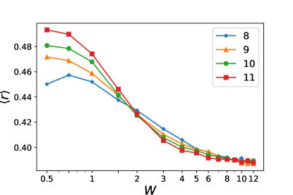
Figure S6: The average ratio of adjacent energy gaps. The system size $N$ is given in the legend. In the thermal phase, the system has Gaussian-orthogonal ensemble (GOE) level statistics while in the many-body localized phase the level statistics follow Poisson distribution. In the main text, we set $W=10$ to make the system deep in the localized phase.

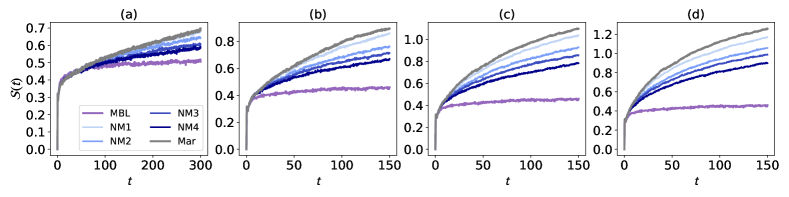
Figure S7: Entanglement entropy of many-body localization dynamics with pure dephasing noise of strength $\lambda=0.3$(a), $\lambda=0.5$(b), $\lambda=0.6$(c), $\lambda=0.8$(d). The purple line shows the results of the clean MBL system. The grey line shows the results under Markovian noise. Blue lines labeled from NM1 to NM4 show the results under non-Markovian noise with non-Markovianity parameter $b=4,1,0.5,0.2$.

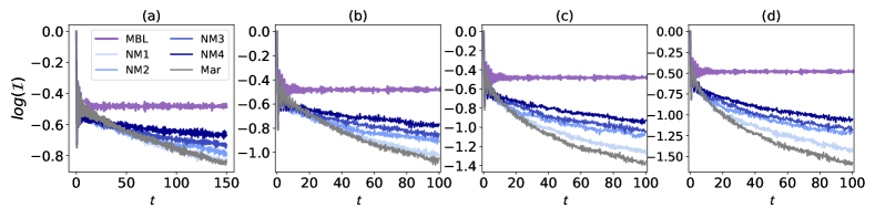
Figure S8: Charge imbalance of many-body localization dynamics with pure dephasing noise of strength $\lambda=0.3$(a), $\lambda=0.5$(b), $\lambda=0.8$(c), $\lambda=1.0$(d). The purple line shows the results of the clean MBL system. The grey line shows the results under Markovian noise. Blue lines labeled from NM1 to NM4 show the results under non-Markovian noise with non-Markovianity parameter $b=4,1,0.5,0.2$.

As explained in the main text, we use the “standard model” for MBL – a one dimensional $S=1/2$ spin chain with nearest neighbor interaction and strong random disorder for on-site potentials - to investigate the dynamics of MBL with and without quantum noise. Note that to be compatible with dephasing noise distribution, the on-site random potential of MBL is chosen to follow the Gaussian distribution $N(0,W/\sqrt{3})$. This distribution gives the same mean and variance values for random variables $W_{i}$ compared to the uniform distribution $U(-W,W)$.

We first study the static property of this model to determine the phase boundary between MBL and thermal phases in terms of the disorder strength $W$. As shown in Fig. S6, we compute the averaged level spacing ratio of the eigenspectrum of the system. The quantity is defined as $\langle r\rangle=\langle\frac{\min\{\delta_{n},\delta_{n+1}\}}{\max\{\delta_{n},\delta_{n+1}\}}\rangle$, where the average $\langle\cdot\rangle$ is defined over different energy level and different disorder configurations, $\delta_{n}=e_{n+1}-e_{n}$ is the adjacent level spacing for eigenstates $e_{n}$. In the MBL phase, the level spacing of the spectrum is expected to follow Possion distribution with no level repulsion $\langle r\rangle\approx 0.386$, while in the thermal phase, the level spacing follows Wigner-Dyson distribution $\langle r\rangle\approx 0.53$. The crossing point of $\langle r\rangle$ of different system sizes corresponds to the delocalization transition point, which is around $W_{c}\approx 2$ in our case. In the dynamical simulation, we set $W=10$ to make the system deeply in the MBL phase.

As explained in the main text, we use entanglement entropy $S$ and the charge imbalance $\mathcal{I}$ to characterize the dynamics. The initial state for the quench dynamics is the $Z_{2}$ product state $|0101....\rangle$. Suppose the stochastically evolved state for a given noise trajectory at the time $t$ is $|\psi(t)\rangle$, charge imbalance is defined as

$$\mathcal{I}(t)=\sum_{i}^{N}(-1)^{i}\langle\psi(t)|S^{z}_{i}|\psi(t)\rangle,$$ (S30)

And the quantity can be further averaged over different disorder realizations.

The half-chain reduced matrix is defined as the partial trace over half of the spin freedom on the evolved pure state under given disorder configurations as $\rho_{A}(t)=\text{Tr}_{B}(|\psi(t)\rangle\langle\psi(t)|)$, where A and B stand for each half chain of the system. The entanglement entropy is thus defined as:

$$S(t)=-\text{Tr}(\rho_{A}(t)\ln\rho_{A}(t)).$$ (S31)

The quantity can be further averaged over different disorder realizations. Note the order here cannot be exchanged due to the non-linear nature of the entropy definition.

Under quantum dephasing noise of different strengths with and without non-Markovianity, we numerically simulate the dynamics using stochastic processes with each time slice $\delta=0.1$ and $500$ disorder configurations. We extract the asymptotic behavior of the two average quantities as summarized in Fig. S7 and Fig. S8.

Note that the charge imbalance is a linear quantity with respect to the state $\rho$, so the computation order (average over different MBL disorder configurations, average over different noise space-time profiles, compute the charge imbalance) doesn’t matter. However, the entanglement entropy depends on the state $\rho$ in a non-linear fashion, so that the computation order in the numerical simulation matters. If we first average over different quantum noise profiles, the resulting state is a mixed state and the entanglement entropy will contain a large part from the thermal fluctuation, failing to capture the intrinsic entanglement. Though in this case, we can utilize other probes such as mutual information or entanglement negativity to determine the intrinsic entanglement components from the averaged mixed state. Instead, we compute the entanglement entropy for each trajectory (each disorder configuration and quantum noise profile), so that the entanglement is all from pure state contribution, reflecting the intrinsic property of the eigenstates of MBL system. This subtle difference in computation order also exists in measurement induced entanglement phase transition studies.

References

- Ashida et al. (2020) Y. Ashida, Z. Gong, and M. Ueda, Non-hermitian physics, Advances in Physics 69, 249 (2020).
- Bergholtz et al. (2021) E. J. Bergholtz, J. C. Budich, and F. K. Kunst, Exceptional topology of non-hermitian systems, Reviews of Modern Physics 93, 015005 (2021).
- Heiss (2012) W. Heiss, The physics of exceptional points, Journal of Physics A: Mathematical and Theoretical 45, 444016 (2012).
- Lee (2016) T. E. Lee, Anomalous edge state in a non-hermitian lattice, Physical review letters 116, 133903 (2016).
- Leykam et al. (2017) D. Leykam, K. Y. Bliokh, C. Huang, Y. D. Chong, and F. Nori, Edge modes, degeneracies, and topological numbers in non-hermitian systems, Physical review letters 118, 040401 (2017).
- Xu et al. (2017) Y. Xu, S.-T. Wang, and L.-M. Duan, Weyl exceptional rings in a three-dimensional dissipative cold atomic gas, Physical review letters 118, 045701 (2017).
- Kunst et al. (2018) F. K. Kunst, E. Edvardsson, J. C. Budich, and E. J. Bergholtz, Biorthogonal bulk-boundary correspondence in non-hermitian systems, Physical review letters 121, 026808 (2018).
- Yao et al. (2018) S. Yao, F. Song, and Z. Wang, Non-hermitian chern bands, Physical review letters 121, 136802 (2018).
- Yao and Wang (2018) S. Yao and Z. Wang, Edge states and topological invariants of non-hermitian systems, Physical review letters 121, 086803 (2018).
- Ingarden et al. (2013) R. S. Ingarden, A. Kossakowski, and M. Ohya, Information dynamics and open systems: classical and quantum approach, Vol. 86 (Springer Science & Business Media, 2013).
- Peres and Terno (2004) A. Peres and D. R. Terno, Quantum information and relativity theory, Reviews of Modern Physics 76, 93 (2004).
- Knill (2005) E. Knill, Quantum computing with realistically noisy devices, Nature 434, 39 (2005).
- Kitaev (1997) A. Y. Kitaev, Quantum computations: algorithms and error correction, Russian Mathematical Surveys 52, 1191 (1997).
- Yoshihara et al. (2006) F. Yoshihara, K. Harrabi, A. Niskanen, Y. Nakamura, and J. S. Tsai, Decoherence of flux qubits due to 1/f flux noise, Physical review letters 97, 167001 (2006).
- Kakuyanagi et al. (2007) K. Kakuyanagi, T. Meno, S. Saito, H. Nakano, K. Semba, H. Takayanagi, F. Deppe, and A. Shnirman, Dephasing of a superconducting flux qubit, Physical review letters 98, 047004 (2007).
- De Lange et al. (2010) G. De Lange, Z.-H. Wang, D. Riste, V. Dobrovitski, and R. Hanson, Universal dynamical decoupling of a single solid-state spin from a spin bath, Science 330, 60 (2010).
- Bar-Gill et al. (2013) N. Bar-Gill, L. M. Pham, A. Jarmola, D. Budker, and R. L. Walsworth, Solid-state electronic spin coherence time approaching one second, Nature communications 4, 1743 (2013).
- Kawakami et al. (2014) E. Kawakami, P. Scarlino, D. R. Ward, F. Braakman, D. Savage, M. Lagally, M. Friesen, S. N. Coppersmith, M. A. Eriksson, and L. Vandersypen, Electrical control of a long-lived spin qubit in a si/sige quantum dot, Nature nanotechnology 9, 666 (2014).
- Watson et al. (2018) T. Watson, S. Philips, E. Kawakami, D. Ward, P. Scarlino, M. Veldhorst, D. Savage, M. Lagally, M. Friesen, S. Coppersmith, et al., A programmable two-qubit quantum processor in silicon, nature 555, 633 (2018).
- Pokharel et al. (2018) B. Pokharel, N. Anand, B. Fortman, and D. A. Lidar, Demonstration of fidelity improvement using dynamical decoupling with superconducting qubits, Physical review letters 121, 220502 (2018).
- Chen et al. (2020) Y.-Q. Chen, K.-L. Ma, Y.-C. Zheng, J. Allcock, S. Zhang, and C.-Y. Hsieh, Non-markovian noise characterization with the transfer tensor method, Physical Review Applied 13, 034045 (2020).
- Breuer et al. (2016) H.-P. Breuer, E.-M. Laine, J. Piilo, and B. Vacchini, Colloquium: Non-markovian dynamics in open quantum systems, Reviews of Modern Physics 88, 021002 (2016).
- Breuer and Petruccione (2002) H.-P. Breuer and F. Petruccione, The theory of open quantum systems (Oxford University Press, USA, 2002).
- Rivas et al. (2010) Á. Rivas, S. F. Huelga, and M. B. Plenio, Entanglement and non-markovianity of quantum evolutions, Physical review letters 105, 050403 (2010).
- Breuer et al. (2009) H.-P. Breuer, E.-M. Laine, and J. Piilo, Measure for the degree of non-markovian behavior of quantum processes in open systems, Physical review letters 103, 210401 (2009).
- Cerrillo and Cao (2014) J. Cerrillo and J. Cao, Non-markovian dynamical maps: numerical processing of open quantum trajectories, Physical review letters 112, 110401 (2014).
- Chen et al. (2022) Y.-Q. Chen, Y.-C. Zheng, S. Zhang, and C.-Y. Hsieh, Spectral-transfer-tensor method for characterizing non-markovian noise, Physical Review Applied 17, 064007 (2022).
- Misra and Sudarshan (1977) B. Misra and E. G. Sudarshan, The zeno’s paradox in quantum theory, Journal of Mathematical Physics 18, 756 (1977).
- Vasile et al. (2011) R. Vasile, S. Olivares, M. A. Paris, and S. Maniscalco, Continuous-variable quantum key distribution in non-markovian channels, Physical Review A 83, 042321 (2011).
- Žnidarič et al. (2011) M. Žnidarič, C. Pineda, and I. Garcia-Mata, Non-markovian behavior of small and large complex quantum systems, Physical review letters 107, 080404 (2011).
- Wakakuwa (2017) E. Wakakuwa, Operational resource theory of non-markovianity, arXiv preprint arXiv:1709.07248 (2017).
- Matsuzaki et al. (2011) Y. Matsuzaki, S. C. Benjamin, and J. Fitzsimons, Magnetic field sensing beyond the standard quantum limit under the effect of decoherence, Physical Review A 84, 012103 (2011).
- Chin et al. (2012) A. W. Chin, S. F. Huelga, and M. B. Plenio, Quantum metrology in non-markovian environments, Physical review letters 109, 233601 (2012).
- Anderson (1958a) P. W. Anderson, Random-phase approximation in the theory of superconductivity, Physical Review 112, 1900 (1958a).
- Basko et al. (2006) D. M. Basko, I. L. Aleiner, and B. L. Altshuler, Metal-insulator transition in a weakly interacting many-electron system with localized single-particle states, Annals of Physics 321, 1126 (2006).
- Zhang et al. (2021) L. Zhang, L. Zhang, and X.-J. Liu, Quench-induced dynamical topology under dynamical noise, Physical Review Research 3, 013229 (2021).
- Lin et al. (2022) Z. Lin, L. Zhang, X. Long, Y.-a. Fan, Y. Li, K. Tang, J. Li, X. Nie, T. Xin, X.-J. Liu, et al., Experimental quantum simulation of non-hermitian dynamical topological states using stochastic schrödinger equation, npj Quantum Information 8, 77 (2022).
- Erlingsson and Nazarov (2002) S. I. Erlingsson and Y. V. Nazarov, Hyperfine-mediated transitions between a zeeman split doublet in gaas quantum dots: The role of the internal field, Physical Review B 66, 155327 (2002).
- Witzel et al. (2014) W. M. Witzel, K. Young, and S. D. Sarma, Converting a real quantum spin bath to an effective classical noise acting on a central spin, Physical Review B 90, 115431 (2014).
- Makri (1999) N. Makri, The linear response approximation and its lowest order corrections: An influence functional approach, The Journal of Physical Chemistry B 103, 2823 (1999).
- Liu et al. (2011) B.-H. Liu, L. Li, Y.-F. Huang, C.-F. Li, G.-C. Guo, E.-M. Laine, H.-P. Breuer, and J. Piilo, Experimental control of the transition from markovian to non-markovian dynamics of open quantum systems, Nature Physics 7, 931 (2011).
- Ma et al. (2014) T. Ma, Y. Chen, T. Chen, S. R. Hedemann, and T. Yu, Crossover between non-markovian and markovian dynamics induced by a hierarchical environment, Physical Review A 90, 042108 (2014).
- Levi et al. (2016) E. Levi, M. Heyl, I. Lesanovsky, and J. P. Garrahan, Robustness of Many-Body Localization in the Presence of Dissipation, Phys. Rev. Lett. 116, 237203 (2016).
- Wybo et al. (2020) E. Wybo, M. Knap, and F. Pollmann, Entanglement dynamics of a many-body localized system coupled to a bath, Physical Review B 102, 064304 (2020).
- Vajna and Dóra (2015) S. Vajna and B. Dóra, Topological classification of dynamical phase transitions, Physical Review B 91, 155127 (2015).
- Caio et al. (2015) M. Caio, N. R. Cooper, and M. Bhaseen, Quantum quenches in chern insulators, Physical review letters 115, 236403 (2015).
- Budich and Heyl (2016) J. C. Budich and M. Heyl, Dynamical topological order parameters far from equilibrium, Physical Review B 93, 085416 (2016).
- Wilson et al. (2016) J. H. Wilson, J. C. Song, and G. Refael, Remnant geometric hall response in a quantum quench, Physical review letters 117, 235302 (2016).
- Fläschner et al. (2018) N. Fläschner, D. Vogel, M. Tarnowski, B. Rem, D.-S. Lühmann, M. Heyl, J. Budich, L. Mathey, K. Sengstock, and C. Weitenberg, Observation of dynamical vortices after quenches in a system with topology, Nature Physics 14, 265 (2018).
- Ünal et al. (2020) F. N. Ünal, A. Bouhon, and R.-J. Slager, Topological euler class as a dynamical observable in optical lattices, Physical review letters 125, 053601 (2020).
- Hu and Zhao (2020) H. Hu and E. Zhao, Topological invariants for quantum quench dynamics from unitary evolution, Physical Review Letters 124, 160402 (2020).
- Sun et al. (2018) W. Sun, C.-R. Yi, B.-Z. Wang, W.-W. Zhang, B. C. Sanders, X.-T. Xu, Z.-Y. Wang, J. Schmiedmayer, Y. Deng, X.-J. Liu, et al., Uncover topology by quantum quench dynamics, Physical review letters 121, 250403 (2018).
- Yi et al. (2019) C.-R. Yi, L. Zhang, L. Zhang, R.-H. Jiao, X.-C. Cheng, Z.-Y. Wang, X.-T. Xu, W. Sun, X.-J. Liu, S. Chen, et al., Observing topological charges and dynamical bulk-surface correspondence with ultracold atoms, Physical review letters 123, 190603 (2019).
- Xin et al. (2020) T. Xin, Y. Li, Y.-a. Fan, X. Zhu, Y. Zhang, X. Nie, J. Li, Q. Liu, and D. Lu, Quantum phases of three-dimensional chiral topological insulators on a spin quantum simulator, Physical Review Letters 125, 090502 (2020).
- Ji et al. (2020) W. Ji, L. Zhang, M. Wang, L. Zhang, Y. Guo, Z. Chai, X. Rong, F. Shi, X.-J. Liu, Y. Wang, et al., Quantum simulation for three-dimensional chiral topological insulator, Physical Review Letters 125, 020504 (2020).
- Niu et al. (2021) J. Niu, T. Yan, Y. Zhou, Z. Tao, X. Li, W. Liu, L. Zhang, H. Jia, S. Liu, Z. Yan, et al., Simulation of higher-order topological phases and related topological phase transitions in a superconducting qubit, Science Bulletin 66, 1168 (2021).
- Zhang et al. (2018) L. Zhang, L. Zhang, S. Niu, and X.-J. Liu, Dynamical classification of topological quantum phases, Science Bulletin 63, 1385 (2018).
- Zhang et al. (2019) L. Zhang, L. Zhang, and X.-J. Liu, Dynamical detection of topological charges, Physical Review A 99, 053606 (2019).
- Zhang et al. (2020) L. Zhang, L. Zhang, and X.-J. Liu, Unified theory to characterize floquet topological phases by quench dynamics, Physical Review Letters 125, 183001 (2020).
- Zhang et al. (2022) L. Zhang, W. Jia, and X.-J. Liu, Universal topological quench dynamics for z2 topological phases, Science Bulletin 67, 1236 (2022).
- Srednicki (1994) M. Srednicki, Chaos and quantum thermalization, Physical Review E 50, 888 (1994).
- Anderson (1958b) P. W. Anderson, Absence of diffusion in certain random lattices, Physical Review 109, 1492 (1958b).
- Serbyn et al. (2013a) M. Serbyn, Z. Papić, and D. A. Abanin, Local Conservation Laws and the Structure of the Many-Body Localized States, Physical Review Letters 111, 127201 (2013a).
- Oganesyan and Huse (2007) V. Oganesyan and D. A. Huse, Localization of interacting fermions at high temperature, Physical Review B 75, 155111 (2007).
- Pal and Huse (2010) A. Pal and D. A. Huse, Many-body localization phase transition, Physical Review B 82, 174411 (2010).
- Nandkishore and Huse (2015) R. Nandkishore and D. A. Huse, Many body localization and thermalization in quantum statistical mechanics, Annual Review of Condensed Matter Physics 6, 15 (2015).
- Altman and Vosk (2015) E. Altman and R. Vosk, Universal Dynamics and Renormalization in Many-Body-Localized Systems, Annual Review of Condensed Matter Physics 6, 383 (2015).
- Abanin et al. (2019) D. A. Abanin, E. Altman, I. Bloch, and M. Serbyn, Colloquium : Many-body localization, thermalization, and entanglement, Reviews of Modern Physics 91, 021001 (2019).
- Iyer et al. (2013) S. Iyer, V. Oganesyan, G. Refael, and D. A. Huse, Many-body localization in a quasiperiodic system, Physical Review B 87, 134202 (2013).
- Khemani et al. (2017) V. Khemani, D. N. Sheng, and D. A. Huse, Two Universality Classes for the Many-Body Localization Transition, Physical Review Letters 119, 075702 (2017).
- Zhang and Yao (2018) S. X. Zhang and H. Yao, Universal Properties of Many-Body Localization Transitions in Quasiperiodic Systems, Physical Review Letters 121, 206601 (2018).
- Zhang and Yao (2019) S.-X. Zhang and H. Yao, Strong and Weak Many-Body Localizations, arXiv:1906.00971 (2019).
- Kohlert et al. (2019) T. Kohlert, S. Scherg, X. Li, H. P. Lüschen, S. Das Sarma, I. Bloch, and M. Aidelsburger, Observation of Many-Body Localization in a One-Dimensional System with a Single-Particle Mobility Edge, Physical Review Letters 122, 170403 (2019).
- Schulz et al. (2019) M. Schulz, C. A. Hooley, R. Moessner, and F. Pollmann, Stark Many-Body Localization, Physical Review Letters 122, 040606 (2019).
- van Nieuwenburg et al. (2019) E. van Nieuwenburg, Y. Baum, and G. Refael, From Bloch oscillations to many-body localization in clean interacting systems, Proceedings of the National Academy of Sciences 116, 9269 (2019).
- Khemani et al. (2020) V. Khemani, M. Hermele, and R. Nandkishore, Localization from Hilbert space shattering: From theory to physical realizations, Physical Review B 101, 174204 (2020).
- Doggen et al. (2021) E. V. H. Doggen, I. V. Gornyi, and D. G. Polyakov, Stark many-body localization: Evidence for Hilbert-space shattering, Physical Review B 103, L100202 (2021).
- Liu et al. (2023a) S. Liu, S.-X. Zhang, C.-y. Hsieh, S. Zhang, and H. Yao, Discrete Time Crystal Enabled by Stark Many-Body Localization, Physical Review Letters 130, 120403 (2023a).
- Else et al. (2020) D. V. Else, C. Monroe, C. Nayak, and N. Y. Yao, Discrete Time Crystals, Annual Review of Condensed Matter Physics 11, 467 (2020).
- Zaletel et al. (2023) M. P. Zaletel, M. Lukin, C. Monroe, C. Nayak, F. Wilczek, and N. Y. Yao, Colloquium : Quantum and classical discrete time crystals, Reviews of Modern Physics 95, 031001 (2023).
- Yang et al. (2020) Z.-c. Yang, F. Liu, A. V. Gorshkov, and T. Iadecola, Hilbert-Space Fragmentation from Strict Confinement, Physical Review Letters 124, 207602 (2020).
- Schreiber et al. (2015) M. Schreiber, S. S. Hodgman, P. Bordia, H. P. Lüschen, M. H. Fischer, R. Vosk, E. Altman, U. Schneider, and I. Bloch, Observation of many-body localization of interacting fermions in a quasi-random optical lattice, Science 349, 842 (2015).
- Smith et al. (2016) J. Smith, A. Lee, P. Richerme, B. Neyenhuis, P. W. Hess, P. Hauke, M. Heyl, D. A. Huse, and C. Monroe, Many-body localization in a quantum simulator with programmable random disorder, Nature Physics 12, 907 (2016).
- Liu et al. (2023b) S. Liu, S.-X. Zhang, C.-Y. Hsieh, S. Zhang, and H. Yao, Probing many-body localization by excited-state variational quantum eigensolver, Physical Review B 107, 024204 (2023b).
- Gong et al. (2021) M. Gong, G. D. de Moraes Neto, C. Zha, Y. Wu, H. Rong, Y. Ye, S. Li, Q. Zhu, S. Wang, Y. Zhao, F. Liang, J. Lin, Y. Xu, C.-z. Peng, H. Deng, A. Bayat, X. Zhu, and J.-W. Pan, Experimental characterization of the quantum many-body localization transition, Physical Review Research 3, 033043 (2021).
- Bardarson et al. (2012) J. H. Bardarson, F. Pollmann, and J. E. Moore, Unbounded growth of entanglement in models of many-body localization, Physical Review Letters 109, 017202 (2012).
- Serbyn et al. (2013b) M. Serbyn, Z. Papić, and D. A. Abanin, Universal Slow Growth of Entanglement in Interacting Strongly Disordered Systems, Physical Review Letters 110, 260601 (2013b).
- Skinner et al. (2019) B. Skinner, J. Ruhman, and A. Nahum, Measurement-Induced Phase Transitions in the Dynamics of Entanglement, Physical Review X 9, 031009 (2019).
- Chan et al. (2019) A. Chan, R. M. Nandkishore, M. Pretko, and G. Smith, Unitary-projective entanglement dynamics, Physical Review B 99, 224307 (2019).
- Li et al. (2018) Y. Li, X. Chen, and M. P. A. Fisher, Quantum Zeno effect and the many-body entanglement transition, Physical Review B 98, 205136 (2018).
- Lashkari et al. (2013) N. Lashkari, D. Stanford, M. Hastings, T. Osborne, and P. Hayden, Towards the fast scrambling conjecture, Journal of High Energy Physics 2013, 22 (2013).
- Sahu and Jian (2023) S. Sahu and S.-k. Jian, Phase transitions in sampling and error correction in local Brownian circuits, arXiv:2307.04267 (2023).
- Zhang et al. (2023) S.-X. Zhang, J. Allcock, Z.-Q. Wan, S. Liu, J. Sun, H. Yu, X.-H. Yang, J. Qiu, Z. Ye, Y.-Q. Chen, C.-K. Lee, Y.-C. Zheng, S.-K. Jian, H. Yao, C.-Y. Hsieh, and S. Zhang, TensorCircuit: a Quantum Software Framework for the NISQ Era, Quantum 7, 912 (2023).
- Biercuk et al. (2009) M. J. Biercuk, H. Uys, A. P. VanDevender, N. Shiga, W. M. Itano, and J. J. Bollinger, Optimized dynamical decoupling in a model quantum memory, Nature 458, 996 (2009).
- Ajoy et al. (2011) A. Ajoy, G. A. Álvarez, and D. Suter, Optimal pulse spacing for dynamical decoupling in the presence of a purely dephasing spin bath, Physical Review A 83, 032303 (2011).
- Cywiński et al. (2008) Ł. Cywiński, R. M. Lutchyn, C. P. Nave, and S. D. Sarma, How to enhance dephasing time in superconducting qubits, Physical Review B 77, 174509 (2008).
- Imamog et al. (1994) A. Imamog et al., Stochastic wave-function approach to non-markovian systems, Physical Review A 50, 3650 (1994).
- Park et al. (2000) S. Park, S. Chuang, J. Minch, and D. Ahn, Intraband relaxation time effects on non-markovian gain with many-body effects and comparison with experiment, Semiconductor science and technology 15, 203 (2000).
- Heideman et al. (1985) M. T. Heideman, D. H. Johnson, and C. S. Burrus, Gauss and the history of the fast fourier transform, Archive for history of exact sciences , 265 (1985).
- Hasan and Kane (2010) M. Z. Hasan and C. L. Kane, Colloquium: topological insulators, Reviews of modern physics 82, 3045 (2010).
- Qi and Zhang (2011) X.-L. Qi and S.-C. Zhang, Topological insulators and superconductors, Reviews of Modern Physics 83, 1057 (2011).
- Chiu et al. (2016) C.-K. Chiu, J. C. Teo, A. P. Schnyder, and S. Ryu, Classification of topological quantum matter with symmetries, Reviews of Modern Physics 88, 035005 (2016).
- Sato and Ando (2017) M. Sato and Y. Ando, Topological superconductors: a review, Reports on Progress in Physics 80, 076501 (2017).
- Landau and Lifshitz (1999) L. Landau and E. Lifshitz, Statistical physics, course theoretical phys., vol. 5 (1999).