HiDiffusion: Unlocking High-Resolution Creativity and Efficiency in Low-Resolution Trained Diffusion Models

Abstract

We introduce HiDiffusion, a tuning-free framework comprised of Resolution-Aware U-Net (RAU-Net) and Modified Shifted Window Multi-head Self-Attention (MSW-MSA) to enable pretrained large text-to-image diffusion models to efficiently generate high-resolution images (e.g. 1024$\times$1024) that surpass the training image resolution. Pretrained diffusion models encounter unreasonable object duplication in generating images beyond the training image resolution. We attribute it to the mismatch between the feature map size of high-resolution images and the receptive field of U-Net’s convolution. To address this issue, we propose a simple yet scalable method named RAU-Net. RAU-Net dynamically adjusts the feature map size to match the convolution’s receptive field in the deep block of U-Net. Another obstacle in high-resolution synthesis is the slow inference speed of U-Net. Our observations reveal that the global self-attention in the top block, which exhibits locality, however, consumes the majority of computational resources. To tackle this issue, we propose MSW-MSA. Unlike previous window attention mechanisms, our method uses a much larger window size and dynamically shifts windows to better accommodate diffusion models. Extensive experiments demonstrate that our HiDiffusion can scale diffusion models to generate 1024$\times$1024, 2048$\times$2048, or even 4096$\times$4096 resolution images, while simultaneously reducing inference time by 40%-60%, achieving state-of-the-art performance on high-resolution image synthesis. The most significant revelation of our work is that a pretrained diffusion model on low-resolution images is scalable for high-resolution generation without further tuning. We hope this revelation can provide insights for future research on the scalability of diffusion models.

Figure 1: High-resolution images generated by HiDiffusion. See Fig. 7 and appendix for more images. Our method enables Stable Diffusion models to generate high-resolution images that surpass the training image size without any further training or fine-tuning. Additionally, our method can significantly reduce the time consumption by 40% to 60% compared with the vanilla Stable Diffusion. Note that the images shown in this paper are compressed due to the file size constraints. We will release the lossless images as soon as possible.

1 Introduction

Generative model has witnessed an explosion of diffusion models of growing capability and applications [42, 10, 43, 41, 34]. Being trained on a large volume of training images (Laion 5B [40]), Stable Diffusion (SD) [34, 29] can generate fixed-size (e.g. 768$\times$768 for SD 2.1 [34]) high-quality images given text or other kinds of prompts. However, it is limited to synthesizing images with higher resolution (e.g. 2048$\times$2048). The limitation has two perspectives: (i) Feasibility. Diffusion models lack scalability in higher-resolution image generation. As illustrated in  Fig. 2, when scaling image resolution from 512$\times$512 to 1024$\times$1024 for SD 1.5 [34], the generated images exhibit unreasonable object duplication and inexplicable object overlaps. (ii) Efficiency. As resolution increases, the time cost becomes more and more unacceptable. For example, SD 1.5 can generate a 512$\times$512 resolution image in only 5s, whereas it takes 182s to generate a 2048$\times$2048 image on an NVIDIA RTX 2080Ti . The low efficiency of diffusion models in high-resolution generation makes it impractical for real-world applications.

Can Stable Diffusion efficiently synthesize images with resolution beyond the training image sizes? Existing methods answer this question by leveraging additional super-resolution models [34, 50], or stacking fix-sized images on a high-resolution canvas [1, 14], or introducing a scaling factor to adjust the attention entropy [15]. However, These approaches either require significant additional training efforts or still suffer from object duplication. By analyzing the components of Stable Diffusion, we find that the receptive field of self-attention consistently equals the resolution, while cross-attention and MLP are both pixel-wise operations. These operations are not sensitive to resolution. However, the receptive field of convolutions remains fixed and does not dynamically adapt to various resolutions. We assume this mismatch makes convolution fail to output structural information of objects suitable for higher resolution.

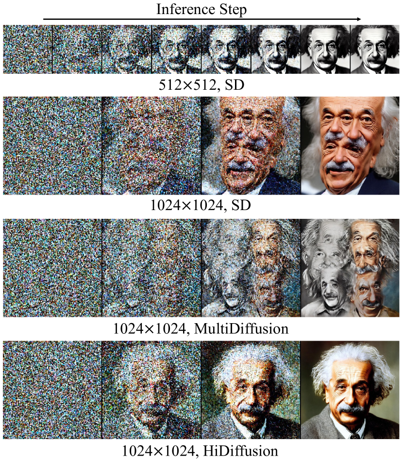
Figure 2: When scaling to 1024$\times$1024 resolution, both SD 1.5 [34] and high-resolution method MultiDiffusion [1] face object duplication in the whole denoising process. Our Hidiffusion is able to generate reasonable object structure and realistic high-resolution images.

To address the mismatch between the feature map size of high-resolution images and the convolution receptive field, we present a simple but effective method called Resolution-Aware U-Net (RAU-Net). Our approach involves Resolution-Aware Downsampler (RAD) and Resolution-Aware Upsampler (RAU) to align the feature map of high-resolution images in the U-Net with the convolution receptive field. The RAD is achieved through a dilated convolution [48] downsampler with a variable dilation rate and stride, which adapts to the desired resolution, while the RAU is achieved through a simple interpolation function. This approach requires no further fine-tuning and can be seamlessly integrated into Stable Diffusion.

Besides high-resolution feasibility, efficiency is another important concern. Many works focus on reducing the sample step [23, 41, 39, 25, 24], while few studies investigate the inference acceleration of diffusion U-Net [2]. These acceleration methods enhance the inference efficiency, but also notably compromise the synthesis image quality. We discover that the time-consuming global self-attention in the top blocks exhibit locality. Inspired by this observation, we propose Modified Shifted Window Multi-head Self-Attention (MSW-MSA) and replace the global self-attention with it in high-resolution synthesis. Note that the substitution needs no further fine-tuning. Compared to window attention used in Swin Transformer [22], our MSW-MSA uses a much larger window size and dynamic shift strides to better accommodate Stable Diffusion.

We integrate RAU-Net and MSW-MSA into one tuning-free framework, dubbed HiDiffusion. To the best of our knowledge, our proposed HiDiffusion is the first to discuss the feasibility and efficiency issues in high-resolution synthesis. We conduct qualitative and quantitative experiments to validate the effectiveness of our method. Specifically, HiDiffusion can scale the synthesis resolution of SD 1.5 [34] and SD 2.1 [34] from 512$\times$512 to 2048$\times$2048 and scale SDXL [29] from 1024$\times$1024 to 4096$\times$4096. Moreover, HiDiffusion reduces the generation time by 40% to 60% compared with vanilla Stable Diffusion in high-resolution image generation. The key finding of our study is that a pretrained diffusion model on low-resolution images can be scaled to high-resolution generation without further fine-tuning. We hope this work can provide valuable guidance for future research on the scalability of diffusion models.

2 Related Work

Text-to-Image Generation. Text-to-image generation (TTI) has emerged as a highly debated and actively researched topic within the thriving field of AI Generated Content (AIGC) [49]. In the early stages, methods [33, 46, 16, 20] based on generative adversarial networks (GANs) [7] primarily utilize the small-scale data regime, effectively generating images through a generator-discriminator structure. More recently, there has been an emerging trend of the Diffusion Models (DMs) to become the new state-of-the-art model in TTI [31, 38, 3, 26]. These auto-regressive methods exploit large-scale data for text-to-image generation, with representative methods such as Stable Diffusion [34], Dreambooth [36], DALL-E [32], demonstrating their remarkable synthesis capabilities. Despite their impressive progress, these methods have limitations in generating high-quality images beyond the resolution of the training images and suffer from high computational costs.

High-Resolution Image Synthesis. Currently, the application of diffusion models in high-resolution image generation poses a significant challenge. Existing methods have primarily concentrated on diffusion in lower-dimensional spaces (latent diffusion) [34], or divided the generative process into multiple training or finetuning sub-problems [14, 44, 12, 45]. For example, Cascaded Diffusion Models [11] employed multiple cascade super-resolution levels of generation. Any-Size-Diffusion [50] introduces a multi-aspect ratio training strategy. Nevertheless, these solutions render the diffusion framework highly intricate. Recently, there has been a growing interest in exploring training-free or tuning-free approaches for variable-sized adaptation. [15] propose a scaling factor from a new perspective of the attention entropy to efficiently improve variable-sized text-to-image synthesis in a training-free manner but not yet addressed the challenge of higher-resolution generation. To tackle this issue, MultiDiffusion [1] manipulated the generation process of a pretrained diffusion model by binding together multiple diffusion generation processes with a shared set of parameters or constraints. SyncDiffusion [17] synchronized multiple diffusions through gradient descent from a perceptual similarity loss. Despite their advancements, these approaches still exhibit object repetition in their results, thereby curbing their overall effectiveness. In contrast, we propose a novel tuning-free method HiDiffusion that not only eradicates the issue of image repetition but also maintains the exceptional fidelity of the generated high-resolution images.

Diffusion Model Acceleration. As diffusion model training and inference is computationally expensive and time-consuming, particularly in the context of high-resolution images, various methods [4, 19, 28] have been extensively investigated to accelerate the training and inference of diffusion models. Unlike fast sampling approaches [41, 43, 39, 23] consider using deterministic sampling schemes to improve the sampling speed. ToMeSD  [2] speeded up an off-the-shelf diffusion model without training by exploiting natural redundancy in generated images by merging redundant tokens. In this work, through the analysis of the locality of global self-attention in the shallow blocks, we develop a novel Modified Shifted Window Multi-head Self-Attention approach that significantly accelerates the generation of high-resolution images without the need for fine-tuning.

3 Method

3.1 Preliminaries

The neural backbone of Stable Diffusion is implemented as a U-Net [5, 35, 34], which contains several Down Blocks, Up Blocks, and a Mid Block, as shown in Fig. 15(a). The Mid Block remains unchanged in our method. Consequently, we omit it for the sake of simplicity. Each Down Block and Up Block can be written respectively as:

$$y =\mathcal{D}(\mathcal{F}(x,t,p),\alpha),$$ (1)

$$y =\mathcal{U}(\mathcal{F}(x,t,p),\beta),\vspace{-5pt}$$ (2)

where $x$ is the input latent feature map, $t$ is the timestep, $p$ is the prompt, $\alpha$ is the downsampling factor, $\beta$ is the upsampling factor. $\mathcal{F}$ incorporates ResNet [8] layers and Vision Transformer [6] layers, which maintain the dimensions of the feature map. $\mathcal{D}(*,\alpha)$ represents the downsampler that downsample the dimensions of the feature map by a factor of $\alpha$, and the upsampler $\mathcal{U}(*,\beta)$ has a similar meaning. $\alpha$ and $\beta$ are set as 2 in vanilla U-Net. The downsampler and upsampler in vanilla U-Net are computed as:

$$\mathcal{D}(x,2)=\mathcal{C}_{3,1,2,1}(x),$$ (3)

$$\mathcal{U}(x,2)=\mathcal{C}_{3,1,1,1}(interp(x,2)),$$ (4)

where $\mathcal{C}_{k,p,s,d}$ means convolution filter with kernel size as $k$, padding size as $p$, stride as $s$, dilation rate as $d$. $interp(x,\beta)$ denotes an interpolation function that upsample the resolution by a factor of $\beta$.

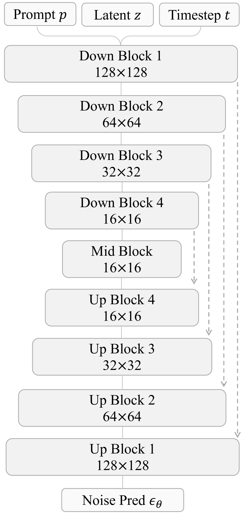
(a) Vanilla U-Net

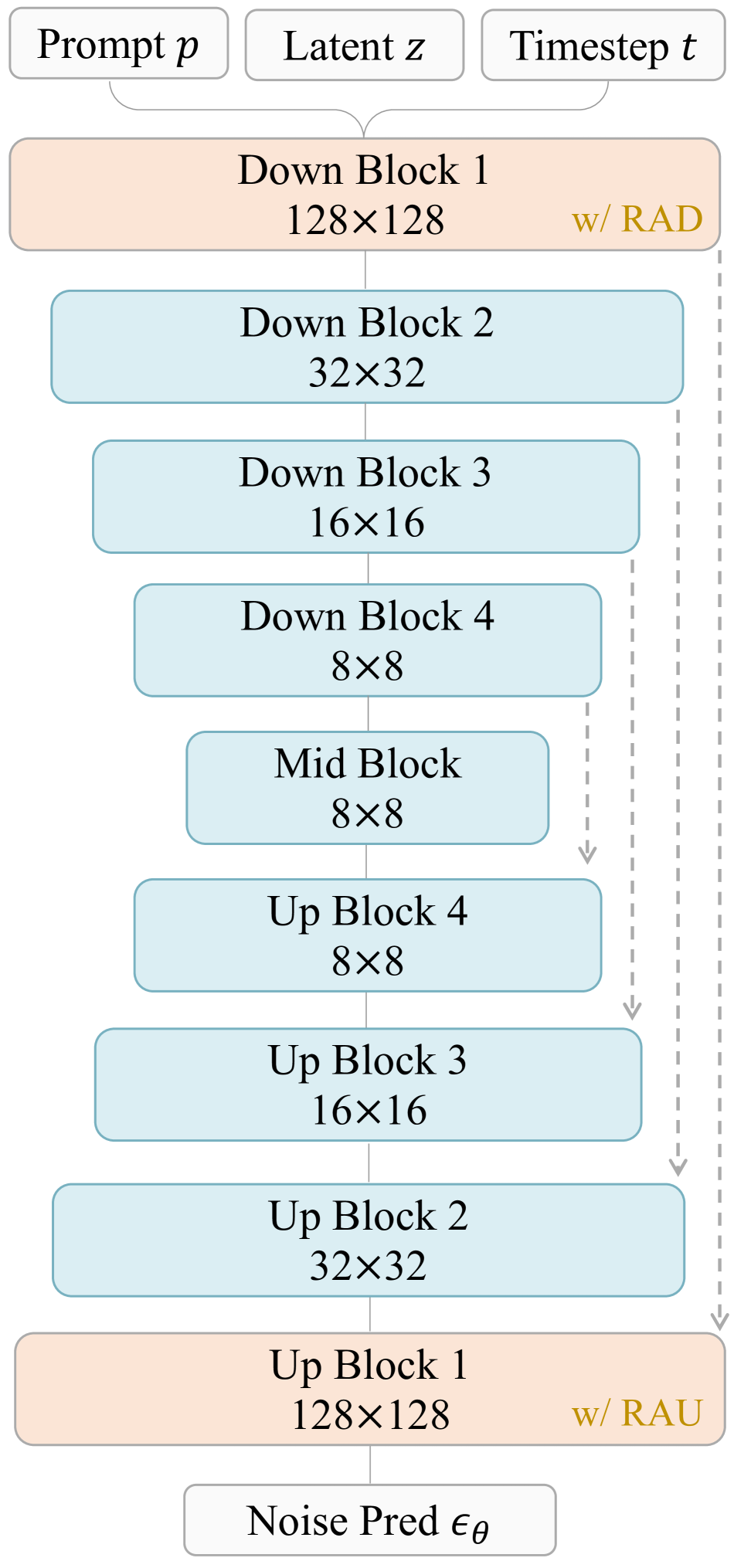
(b) HiDiffusion RAU-Net

Figure 3: Comparison between vanilla Stable Diffusion’s U-Net architecture and our proposed HiDiffusion RAU-Net architecture. Parameters in all blocks are frozen. The main difference lies in the blue Blocks (differ in the dimensions of feature map) and orange Blocks (Our proposed RAD and RAU modules are incorporated into Block 1.).

3.2 HiDiffusion

In the following, we delve into our proposed efficient high-resolution image generation framework, named HiDiffusion. Specifically, our framework comprises two key components: Resolution-Aware U-Net (RAU-Net) and Modified Shifted Window Multi-head Self-Attention (MSW-MSA). The RAU-Net is designed to overcome the drawback of Stable Diffusion in object duplication and inexplicable object overlaps when scaling to higher image resolution, such as 1024 $\times$ 1024. MSW-MSA is introduced to improve the inference efficiency of Stable Diffusion for high-resolution image synthesis. The overall framework of HiDiffusion is present in Fig. 4. We introduce our methods by exemplifying how to enable SD 1.5 to generate images with 1024$\times$1024 resolution. For more extreme resolution, e.g. 2048$\times$2048, please refer to the appendix for detail.

3.2.1 Resolution-Aware U-Net

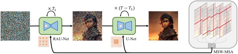
Figure 4: The framework of HiDiffusion.

An illustrative comparison of the vanilla Stable Diffusion (V1.5) U-Net and RAU-Net in the context of generating 1024$\times$1024 resolution images is presented in Fig. 15. We incorporate our Resolution-Aware Downsapler (RAD) in Down Block 1 as a substitute for the conventional downsampler, and likewise, we replace the upsampler with the Resolution-Aware Upsampler (RAU) in Up Block 1. RAD downsamples the feature map to guarantee the dimensions of the resulting feature map align with those of the corresponding training images, thereby matching with the convolution’s receptive field. Specifically, the RAD and RAU can be written as follows:

$$\mathcal{RAD}(x,\alpha)=\mathcal{C}_{3,p,\alpha,d}(x),$$ (5)

$$\mathcal{RAU}(x,\beta)=\mathcal{C}_{3,1,1,1}(interp(x,\beta)).$$ (6)

For 1024$\times$1024 image generation, we need to downsample the feature map by a factor of 4 to match the receptive field of the following convolutions, i.e., $\alpha=4$. This downsampling factor represents twice the downsampling factor of the conventional downsampler. To mitigate information loss caused by the convolutional stride larger than the kernel size, we incorporate dilation by setting $d=2$ and $p=2$. In this case, the effective window size of the convolution in RAD increases from 3 to 5. For RAU, we only need to adjust the interpolation factor to 4. Compared to Vanilla U-Net, both RAD and RAU do not introduce additional trainable parameters. Therefore, RAD and RAU can directly load the weight of the corresponding samplers from Vanilla U-Net without further fine-tuning.

Upon incorporating RAU-Net into SD 1.5, We address the object duplication problem but also bring blurriness. We find that Stable Diffusion forms object structure in the early denoising stage, and refines object details in the later stage. The same phenomenon is also observed in [47]. We discover that RAU-Net can generate rational object structures in the early stage, whereas applying Vanilla U-Net in the later stages can produce more enriching details. Consequently, we establish a threshold $T_{1}$, such that when the denoising steps $t<T_{1}$, RAU-Net is employed, conversely, when the denoising steps $t\geq T_{1}$, Vanilla U-Net is utilized. This simple adjustment can effectively improve the quality of high-resolution images. Moreover, we observed that the parameter $T_{1}$ is not sensitive, with settings between 20 and 40 for 1024 $\times$ 1024 generation yielding notably superior performance. For a detailed comparative analysis of this observation, please refer to Sec. 5.1.

3.2.2 Modified Shifted Window Attention

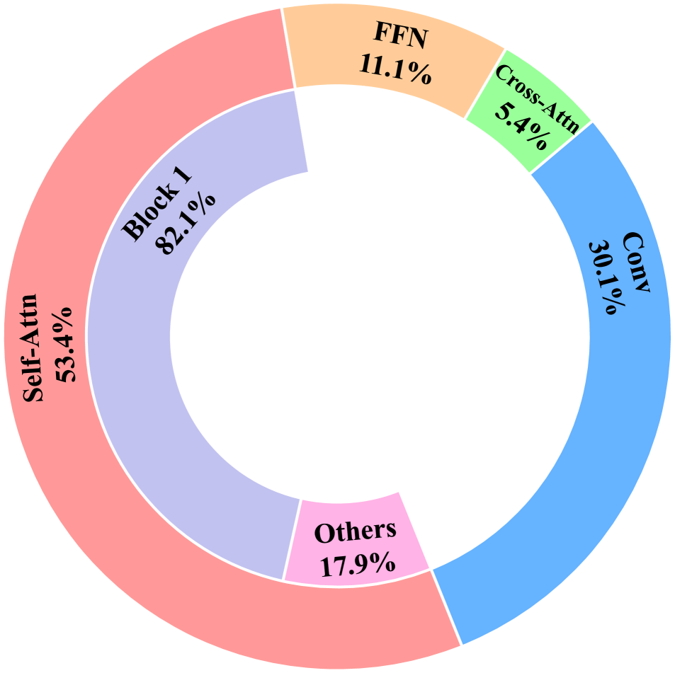
(a) Operation consumption.

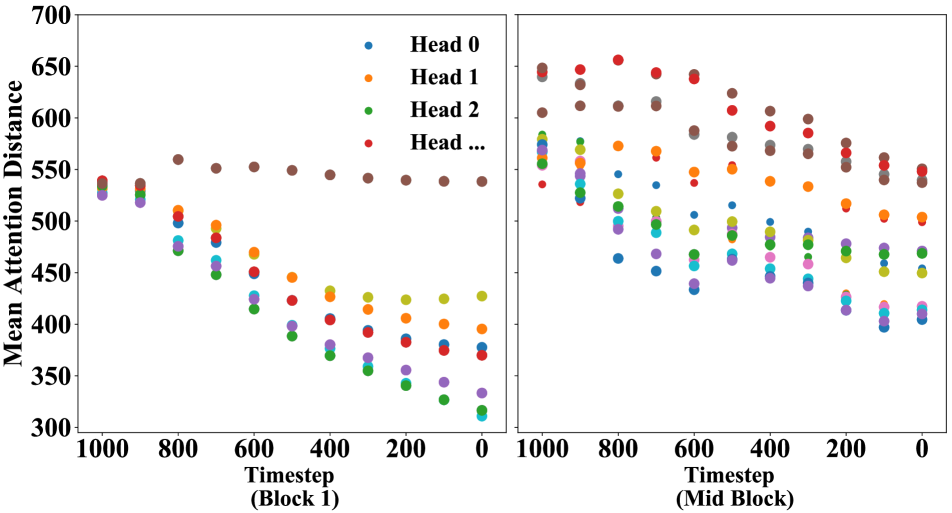
(b) Mean attention distance.

Figure 5: Analysis of the time consumption and mean attention distance. (a) The self-attention operation within Block 1 significantly dominates the time consumption. (b) A pronounced locality is evident in the self-attention mechanism within the top blocks.

Stable Diffusion combined with RAU-Net is capable of generating high-quality high-resolution images. However, it still faces an efficiency challenge: unaffordable slow speed in generating high-resolution images.  Fig. 5(a) shows the time consumption of each operation in SD 1.5, given a latent feature map with 128$\times$128 (corresponding to 1024$\times$1024 resolution in pixel space). It can be observed that self-attention, especially in Block 1 (i.e. Down Block 1 and Up Block 1), takes the dominant consumption, which is also mentioned in [29]. Driven by previous local self-attention works in vision [22, 27], We visualize the mean attention distance for each head across different timesteps of Block 1 (top block) and Mid Block (bottom block), as shown in Fig. 5(b). We surprisingly find that the self-attention mechanism in the top blocks demonstrates a pronounced locality. Certain heads are observed to attend to approximately half of the image, while others focus on even more confined regions close to the query location. According to this observation, it is suggested to propose local self-attention for efficient computation. Specifically, we introduce window attention [22] to replace the original global attention:

$$y=\text{W-MSA}(x,w)+x,$$ (7)

where W-MSA means Window Multi-head Self-Attention and $w$ represents the window size. Besides W-MSA, a window shift operation is also needed to introduce cross-window connections. However, Swin Transformer [22] block that encompasses two successive self-attention modules is incompatible with Stable Diffusion transformer block which includes only one self-attention module. To address this issue, we propose to shift different strides based on the timesteps. Generally, this Modified Shifted Window Multi-head Self-Attention (MSW-MSA) can be written as:

$$y=\text{MSW-MSA}(x,w,s(t))+x,$$ (8)

where $s(t)$ is the shifted stride function dependant on the timestep $t$. Specifically, we adopt a simple yet effective random selection strategy, where at each timestamp, we randomly select a stride parameter from a fixed set of shift strides. This approach enables the integration of information from diverse windows, yielding significant image quality improvement. In comparison to the small window of Swin Transformer [22], another notable modification we have implemented is based on the discovery that larger window sizes are crucial in achieving a favorable balance between efficiency and quality, see Sec. 5.3.

We finally substitute the global self-attention in Block 1 with MSW-MSA. It is worth noting that while other blocks can integrate MSW-MSA, the resulting efficiency gains are not substantial. Experiments demonstrate that our MSW-MSA approach can reduce time consumption by a remarkable 40% to 60% in high-resolution image synthesis.

4 Experiments

4.1 Experiment Settings

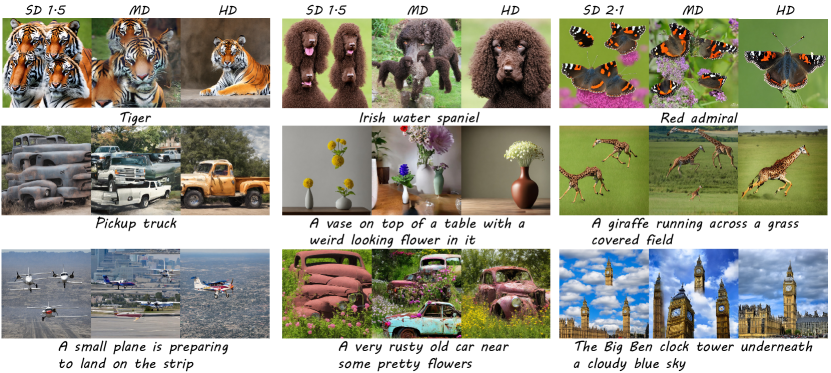
Figure 6: Images with 1024$\times$1024 resolution generated by SD 1.5, SD 2.1, Multidiffusion (MD) and our method HiDiffusion (HD) on ImageNet and COCO datasets. The text beneath each image is the input text prompt for the diffusion model. Please refer to the appendix for more samples.

In this work, we evaluate the performance of our HiDiffusion in SD 1.5 [34], SD 2.1 [34] and SDXL [29]. We apply our approach to text-guided image synthesis on high-resolution, ranging from 4$\times$ to even 16$\times$ times the training image resolution. For quantitative evaluation, we use Frechet Inception Distance (FID) [9] to measure the realism of the output distribution and CLIP Score [30] to evaluate the alignment between image and text. In addition, we utilize the Variance of the Laplacian [13] to evaluate the sharpness of the images, commonly used in image quality assessment. We compare our HiDiffusion with other methods on ImageNet [37] and COCO [21] datasets. Without further elaboration, we generate 10K (10 per class) images to compute metrics for ImageNet evaluation and generate 40,504 (1 per caption) images from COCO 2014 validation captions to compute metrics for COCO evaluation. We use xFormers [18] by default. The model’s latency is measured on a single NVIDIA RTX 2080Ti with a batch size of 1.

We mainly introduce the parameter setting for SD 1.5 and SD 2.1, please refer to the appendix for the SDXL parameter setting. For 1024$\times$1024 generation, we incorporate RAD and RAU in Block 1 and set $\alpha=\beta=4$. We set the window size as $(64,64)$. The predefined set of shift strides is $\{(0,0),(16,16),(32,32),(48,48)\}$. All experiments are conducted with 50 DDIM steps. The classifier-free guidance scale is 7.5. The threshold $T_{1}$ switching from RAU-Net to vanilla U-Net is set as $20$. When extended to 2048$\times$2048, we can simply set $\alpha=8$ to generate images of even higher resolution. However, a sharp change in resolution caused by interpolation may bring blurriness, hence we adopt a progressive approach by incorporating RAU and RAD with $\alpha=\beta=4$ into Block 1 and Block 2, respectively, This allows the feature map to gradually match the receptive field of the convolution. Please refer to the appendix for more details.

ImageNet COCO Method Resolution Latency (s) $\downarrow$ FID $\downarrow$ CLIP Score $\uparrow$ FID $\downarrow$ CLIP Score $\uparrow$ SD 1.5 1024 $\times$ 1024 20.13 25.55 0.295 38.21 0.309 SD 1.5 + HiDiffusion 12.21(-39%) 21.81 0.307 21.36 0.323 SD 2.1 16.77 24.63 0.299 31.33 0.314 SD 2.1 + HiDiffusion 9.89(-41%) 22.34 0.309 20.77 0.326 SD 1.5 2048 $\times$ 2048 182.26 53.03 0.284 78.53 0.286 SD 1.5 + HiDiffusion 74.09(-59%) 27.33 0.307 28.93 0.321 SD 2.1 133.93 60.60 0.281 82.74 0.289 SD 2.1 + HiDiffusion 56.35(-58%) 30.67 0.305 32.87 0.320 SDXL 96.70 27.48 0.300 28.71 0.318 SDXL + HiDiffusion 79.96(-17%) 22.22 0.314 20.89 0.332 SDXL^† 4096 $\times$ 4096 913.16 96.36 0.276 161.68 0.271 SDXL + HiDiffusion^† 666.56(-27%) 64.05 0.299 108.18 0.300

Table 1: Comparison of vanilla Stable Diffusion and our Hidiffusion in zero-shot text-guided image synthesis on ImageNet and COCO dataset. ^† means we generate 5K images for quantitative evaluation due to the heavy computational burden.

4.2 Main results

In this section, We incorporate our method into SD 1.5 [34], SD 2.1 [34], and SDXL [29] to evaluate its effectiveness. SD 1.5 and SD 2.1 are capable of generating images with 512$\times$512 resolution. We integrate our method into them to scale the resolution to 1024$\times$1024 and even 2048$\times$2048. For SDXL, which is trained for generating 1024$\times$1024 images, we incorporate our method to scale the resolution to 2048$\times$2048 and even 4096$\times$4096. Besides fixed aspect ratios, we also generate images with various aspect ratios, such as 512$\times$2048, 1280$\times$1024 and 2048$\times$4096, and so on. We also compare our method with the high-resolution generation method MultiDiffusion (MD) [1]. For the acceleration of the diffusion model, we compare the diffusion acceleration method ToMeSD [2] with our proposed MSW-MSA. Moreover, we compare our method with super-resolution method for a thorough evaluation, even though the latter requires a large number of high-resolution images and extra training efforts to train a super-resolution model.

ImageNet COCO Method Resolution Latency (s) $\downarrow$ FID $\downarrow$ CLIP Score $\uparrow$ FID $\downarrow$ CLIP Score $\uparrow$ SD 1.5 + MD 1024 $\times$ 1024 346.75 24.87 0.301 67.49 0.319 SD 1.5 + HiDiffusion 12.21(-96%) 24.80 0.307 53.70 0.320 SD 2.1 + MD 323.59 24.01 0.302 67.08 0.319 SD 2.1 + HiDiffusion 9.89(-97%) 25.08 0.309 52.99 0.323 SD 1.5 + MD 2048 $\times$ 2048 2673.09 58.59 0.296 119.49 0.298 SD 1.5 + HiDiffusion 74.09(-97%) 29.92 0.307 57.35 0.320 SD 2.1 + MD 2494.02 57.87 0.297 124.43 0.299 SD 2.1 + HiDiffusion 56.35(-98%) 33.04 0.305 59.78 0.316

Table 2: Comparison of high-resolution generation method and our HiDiffusion in zero-shot text-guided image synthesis performance on ImageNet and COCO dataset.

Method	Resolution	Latency (s)	FID $\downarrow$	CLIP-Score $\uparrow$
Baseline	512$\times$ 512	4.63	17.68	0.308
ToMeSD		4.04(-12%)	18.82	0.307
MSW-MSA		4.07(-12%)	16.71	0.308
Baseline	1024$\times$1024	16.37	22.93	0.307
ToMeSD		12.61(-23%)	22.76	0.305
MSW-MSA		12.21(-24%)	21.80	0.307

Table 3: Quantitative evaluation of ToMeSD and our proposed MSW-MSA on ImageNet.

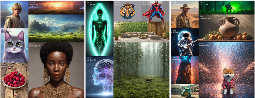
Figure 7: Samples for user-defined text prompts from HiDiffusion. The text displayed in the image represents the diffusion model version and image resolution. After integrating our method, Stale diffusion is capable of efficiently generating high-resolution images with resolutions ranging from 1024$\times$1024 to 4096$\times$4096, accommodating various aspect ratios. Best viewed when zoomed in.

Comparision with vanilla SD. In Fig. 6, we show qualitative comparison between the baseline and our method on ImageNet [37] and COCO [21] datasets. It can be easily seen the vanilla Stable Diffusion suffer from duplication problem and degradation in visual quality as well. In contrast, our HiDiffusion mitigates the duplication problem and holds more realistic image structures simultaneously. We also present samples with user-defined imaginative prompts and extreme resolution with various aspect ratios in Fig. 7. The quantitative results are shown in Tab. 1. Our approach outperforms vanilla SD in both quality and image-text alignment. We achieve much better metric scores across all experiment settings, especially for the images with much higher resolution (a significant FID improvement from 78.53 to 28.93 for SD 2.1 on the resolution 2048$\times$2048).

Laplacian Variance Method Resolution Latency (s) $\downarrow$ FID $\downarrow$ CLIP Score $\uparrow$ Mean $\uparrow$ Max $\uparrow$ SD 1.5 + LDM-SR^∗ 1024 $\times$ 1024 19.82 17.56 0.307 0.486 10.353 SD 1.5 + HiDiffusion 12.21(-38%) 21.81 0.307 0.894 14.027 SD 2.1 + LDM-SR^∗ 19.63 18.54 0.308 0.456 5.387 SD 2.1 + HiDiffusion 9.89(-50%) 22.34 0.309 0.673 13.666 SD 1.5 + LDM-SR^∗ 2048 $\times$ 2048 68.78 17.32 0.308 0.354 6.650 SD 1.5 + HiDiffusion 74.09 27.33 0.307 0.754 15.058 SD 2.1 + LDM-SR^∗ 68.61 18.16 0.308 0.355 5.987 SD 2.1 + HiDiffusion 56.35(-18%) 30.67 0.304 0.579 8.796

Table 4: Comparison of diffusion super-resolution and our method on ImageNet dataset. ^∗ is a two-stage method, requiring extra high-resolution datasets and training efforts to train a large super-resolution model. Our approach is one-stage and can generate high-resolution images without any extra costs.

Comparison with high-resolution synthesis method. In Fig. 6, we present a set of samples for the qualitative comparison between MultiDiffusion (MD) and our method on ImageNet [37] and COCO [21] datasets. We observe that MD fails to mitigate the issue of duplication. Moreover, the images generated by MD fail to adhere to fundamental principles of perspective, wherein objects appear smaller as they get far away. For example, when considering the image generated by MD with the prompt ”A giraffe running across a grass-covered field”, a small-sized deer appears in the foreground while a large-sized deer appears in the background, which deviates from reality. Conversely, our method significantly surpasses MD in terms of both image quality and image structural rationality. Tab. 2 shows quantitative results between MD and our method. Note that we generate 5K images for quantitative evaluation in this section due to the heavy computational burden of MD. The quantitative demonstrates our method outperforms MD across almost all metrics. It is worth noting that we significantly surpass MD in generation efficiency: the latency of our method is only approximately 1/30 of MD.

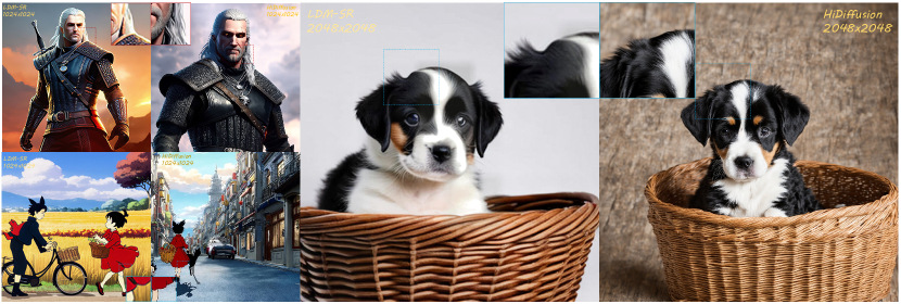
Figure 8: Samples of 1024$\times$1024 and 2048$\times$2048 resolution generated by LDM-SR and our method based on SD 2.1. Please refer to the appendix for more samples.

Comparison with diffusion acceleration method. We compare our method with the widely used diffusion model acceleration technique called Token Merge for Stable Diffusion (ToMeSD) [2]. We compare ToMeSD with our method at the resolutions of 512$\times$512 and 1024$\times$1024 based on SD 1.5.  Tab. 3 shows the quantitative results on ImageNet [37]. As observed, our proposed MSW-MSA outperforms ToMeSD across all metrics. Please refer to the appendix for the visual sample comparison.

Comparison with diffusion super-resolution models. Instead of directly generating high-resolution images using a single diffusion model, a more commonly used approach in the community is to generate 512$\times$512 images using Stable Diffusion and scale them to higher resolution using an extra super-resolution model. Although the latter approach requires additional high-resolution training datasets and extensive training efforts to train a large super-resolution model, we compare it for a thorough comparison, despite the inherent unfairness to our one-stage and training-free method. We compare our method with a pretrained Stable Diffusion super-resolution model LDM-SR [34]  Tab. 4 shows the quantitative results. In terms of generation efficiency, our method outperforms LDM-SR significantly at 1024x1024 resolution (9.89s vs. 19.63s), while it is comparable with LDM-SR at 2048x2048 resolution. Both LDM-SR and our method are capable of generating plausible structures. However, our method exhibits significantly better Laplacian variance across different resolutions. This indicates that the images generated by our method are clearer and more detailed. We visualizing the synthesized samples in Fig. 8. Compared with LDM-SR, a distinction can be observed in terms of visual image quality. Our method directly generates content on a 1024$\times$1024 or 2048$\times$2048 canvas, resulting in higher richness, sharper characteristics, and fine-grained details.

5 Ablation study

5.1 The impact of threshold $T_{1}$ in RAU-Net

$T_{1}$	0	10	20	30	40	50
FID	26.38	24.05	21.81	21.18	21.12	25.55
CLIP-Score	0.309	0.308	0.307	0.308	0.307	0.295

Table 5: Quantitative evaluation of the impact of various $T_{1}$ on the performance of HiDiffusion.

This threshold introduced in Sec. 3.2.1 determines when to switch from RAU-Net to vanilla U-Net. We explore the impact of different thresholds on the performance of HiDiffusion. The quantitative results based on SD 1.5 are shown in Tab. 5. When $T_{1}$ is between 20 and 40, there is no significant difference in metric evaluation. Based on the observation of generated samples, we find that $T_{1}$ ranging from 20 to 40 can effectively alleviate object duplication, with $T_{1}=20$ yielding the optimal performance. Therefore, we select $T_{1}=20$ as the default setting. Please refer to the appendix for visual samples.

5.2 The impact of the position of RAD and RAU

Position	Block 1	Block 2	Block 3
FID	21.81	20.84	21.26
CLIP-Score	0.307	0.307	0.305

Table 6: Quantitative evaluation of the position of RAD and RAU.

Our main idea is to introduce RAD and RAU to dynamically downsample the feature map to match the receptive field of the convolution. We insert the RAD and RAU into Block 1, Block 2, and Block 3 respectively based on SD 1.5 to examine the impact of the Resolution-aware sampler at different locations, as shown in Tab. 6. There is a minor quantitative metric difference between different locations. However, we visually observe that incorporating RAD and RAU in Block 1 can better mitigate object duplication. We present a comparison of the generated samples in the appendix.

5.3 The impact of the window size

The window size determines the receptive field of self-attention. We compare the performance from small window size proposed in Swin Transformer [22] to our proposed large window size based on SD 1.5, as shown in Tab. 7. As the window size gradually increases, the performance improves. We achieve the optimal balance between efficiency and performance when the window size is half the height and width of the feature map.

Window size	4	16	32	64
FID	417.15	53.02	22.37	21.81
CLIP-Score	0.225	0.295	0.307	0.307

Table 7: Quantitative evaluation of the impact of window size.

6 Conclusion

In this paper, we propose a tuning-free framework named HiDiffusion for pretrained text-to-image diffusion models. HiDiffusion includes Resolution-Aware U-Net (RAU-Net) that makes high-resolution generation possible and Modified Shifted Window Multi-head Self-Attention (MSW-MSA) that makes high-resolution generation efficient. Empirically, HiDiffusion can scale diffusion models to generate 1024$\times$1024, 2048$\times$2048, or even 4096$\times$4096 resolution images, while simultaneously reducing inference time by 40%-60%. Compared to super-resolution methods, Our generated images have higher richness and fine-grained details. We hope our work can bring insight to future works about the scalability of diffusion models.

Limitations and future work: Our approach involves directly harnessing the intrinsic potential of stable diffusion without any additional training or fine-tuning, hence some inherent issues posed by stable diffusion persist, such as the requirement for prompt engineering to obtain more promising images. Furthermore, we can explore better ways to integrate with super-resolution models to achieve higher resolution and amazing image generation outcomes.

Appendix

In the appendix, we present the following details associated with HiDiffusion:

• Unsuccessful trials on object duplication.

• Details about SDXL [29] settings.

• Details about extreme resolutions (2048$\times$2048 for SD 1.5 [34], SD 2.1 [34], 4096$\times$4096 for SDXL).

• Ablations on resolution-aware operation.

• Ablations on shift window.

• Additional qualitative results.

Appendix A Unsuccessful trials on object duplication

Solving object duplication problem in high-resolution generation is not a straightforward task. Before effectively addressing it, we went through numerous failed attempts. In this section, we outline three unsuccessful trials that are easily conceived and intuitively viable.

A.1 Latent feature rescale

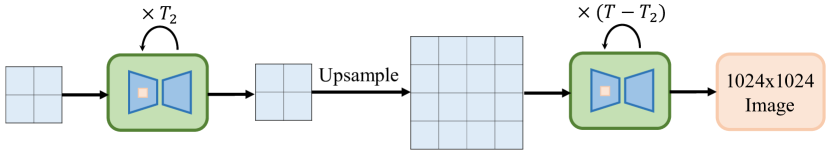
Figure 9: The framework of latent feature rescale.

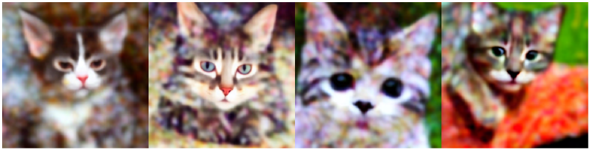
Figure 10: The generated samples of latent feature rescale.

Taking the generation of 1024$\times$1024 resolution images by SD 1.5 [34] as a case study. One straightforward approach to solving object duplication is to first denoise the latent features corresponding to the 512$\times$512 resolution. After denoising certain steps ($T_{2}$), the latent features are upsampled to the size corresponding to 1024$\times$1024 resolution and the denoising process continues, as illustrated in Fig. 9. This method treats the low-resolution latent features at $T_{2}$ timestep as priors to govern the generation content of 1024$\times$1024 resolution. For 50 DDIM steps, we set $T_{2}=30$. The generated samples are shown in Fig. 10, we find that this method fails to generate high-quality 1024$\times$1024 images.

A.2 Low-resolution latent feature guidance

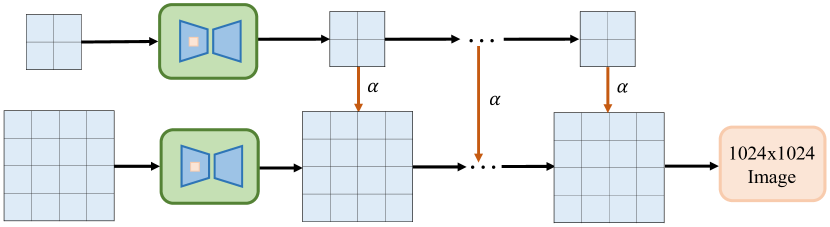
Figure 11: The framework of low-resolution latent feature guidance.

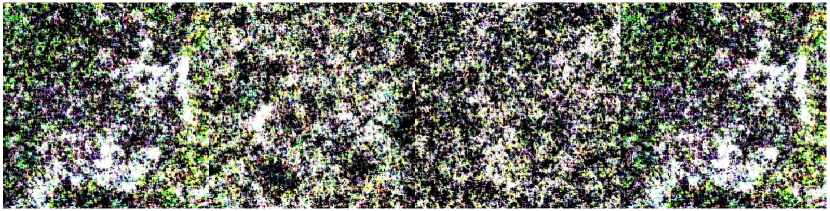
Figure 12: The generated samples of low-resolution latent feature guidance.

As Stable Diffusion can generate reasonable object structures in 512$\times$512 resolution, a straightforward approach involves using the low-resolution (i.e. 512$\times$512) denoising process to guide the high-resolution (i.e. 1024$\times$1024) denoising process, as show in Fig. 11. Assuming that at step $T_{3}$, the latent noise prediction for the 512$\times$512 resolution is denoted as $\epsilon_{l}$, and the latent noise prediction for the 1024$\times$1024 resolution is denoted as $\epsilon_{h}$. We use $\epsilon_{l}$ to guide the direction of $\epsilon_{h}$ by employing a weighted sum:

$$\epsilon_{h}=\alpha\cdot interp(\epsilon_{l},2)+(1-\alpha)\cdot\epsilon_{h}.$$ (9)

We set $\alpha=0.8$ and  Fig. 12 shows the generated samples. We discover that the method even fails to generate structural information about objects. Instead, it still generates images with a large amount of noise.

A.3 Self-attention with fixed receptive field

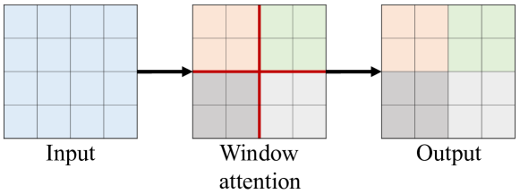
Figure 13: Constrain the receptive field of self-attention by using window attention.

In the main paper, we demonstrate that the receptive field of self-attention is equal to the size of the latent feature. In principle, self-attention with a global receptive field would not be accountable for object duplication. However, we hypothesize that self-attention might be limited to handling interactions within a feature map corresponding to higher resolution. As the generated resolution increases, the number of entries involved in self-attention would increase dramatically, which could result in uncontrollable outcomes. In this section, we maintain the same number of entries for self-attention as during training when generating images with 1024$\times$1024 resolution. This can be achieved by window attention, as shown in Fig. 13. Note that we also introduce shifted window attention as proposed in the main paper. We present the generated samples in Fig. 14. Constraining the receptive field of self-attention cannot solve the object duplication problem. However, when downsampling the feature map to align with the receptive field of convolution, we notice that object duplication disappears. Consequently, we infer that the origin of object duplication is not rooted in self-attention but rather in convolution.

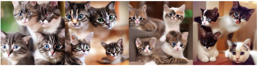
Figure 14: The generated samples when constraining the receptive field of self-attention.

Appendix B Details about SDXL settings.

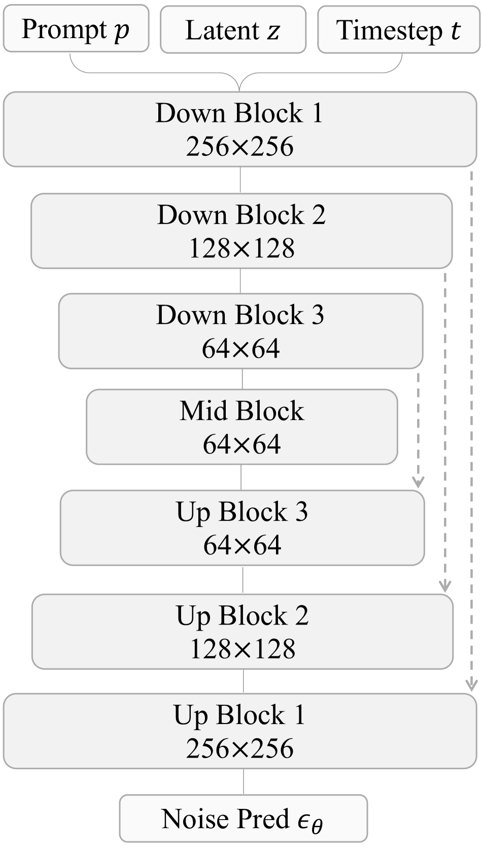
(a) Vanilla U-Net of SDXL

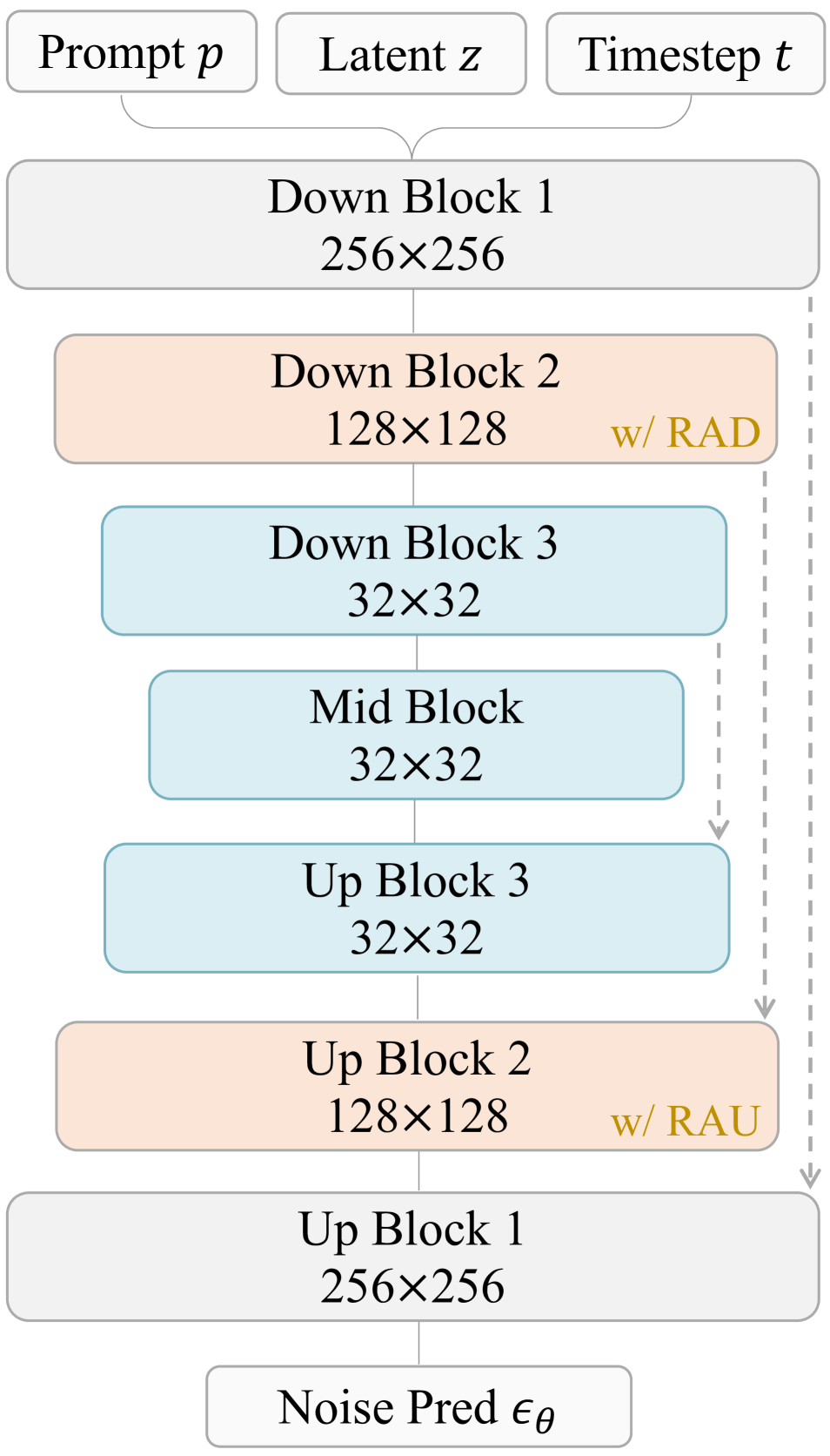
(b) HiDiffusion RAU-Net of SDXL

Figure 15: Comparison between vanilla SDXL’s U-Net and our proposed HiDiffusion RAU-Net for SDXL. Parameters in all blocks are frozen. The main difference lies in the blue Blocks (differ in the dimensions of feature map) and orange Blocks (Our proposed RAD and RAU modules are incorporated into Block 2.).

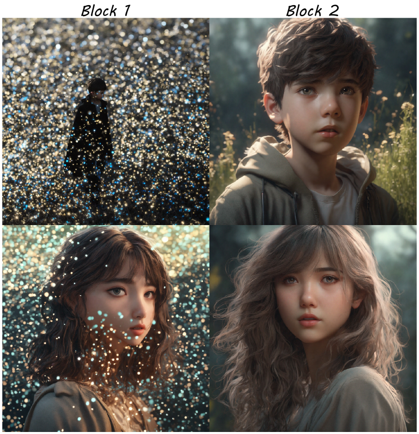
Figure 16: 2048$\times$2048 resolution comparison between inserting resolution-aware samplers into Block 1 and Block 2.

An illustrative comparison of the vanilla SDXL U-Net and RAU-Net for SDXL in the context of generating 2048$\times$2048 resolution images is presented in Fig. 15. We incorporate RAD and RAU in Block 2 and set $\alpha=\beta=4$ to match the receptive field of the following convolutions. In contrast to SD 1.5 and SD 2.1’s U-Net, the Down Block 1 and Up Block 1 of SDXL only consist of two and three ResNet blocks, respectively. If we choose to incorporate the RAD and RAU in Block 1, the shallow ResNet Blocks in Block 1 are insufficient to effectively handle the resolution change caused by the interpolation function in RAD, resulting in the synthesis of blurry images. We present the qualitative comparison between inserting RAD and RAU in Block 1 and inserting RAD and RAU in Block 2 in Fig. 16. In the experiment of the main paper, We set $T_{1}=20$ for 50 DDIM steps. The classifier-free guidance scale is 7.5. Since Block 1 of SDXL U-Net does not contain self-attention, we incorporate MSW-MSA into Block 2. We set the window size as $(64,64)$. The predefined set of shift strides is $\{(0,0),(16,16),(32,32),(48,48)\}$. For 4096$\times$4096 resolution generation, please refer to Appendix C.

Appendix C Details about extreme resolutions

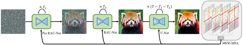
Figure 17: The framework of image synthesis with extreme resolution (2048$\times$2048 for SD 1.5 and SD 2.1, 4096$\times$4096 for SDXL). Pro RAU-Net means progressive RAU-Net.

For SD 1.5 and SD 2.1, generating images with 2048$\times$2048 resolution is a significant challenge, considering that this resolution is already 16 times the training image resolution. RAU-Net can generate images with 2048$\times$2048 resolution by simply setting $\alpha=\beta=8$, $d=4$, $p=4$, as shown in Fig. 18(b). However, $\beta=8$ implies that RAU upsamples the feature map by a factor of 8 using an interpolation function. This abrupt resolution change brought by interpolation leads to the generation of blurred images, as illustrated in Fig. 20(a). To tackle the issue of declining image quality in extreme resolution, we adopt a progressive variant of RAU-Net, as shown in Fig. 18(c). We incorporate RAU and RAD with $\alpha=\beta=4$, $d=2$, $p=2$ into Block 1 and Block 2, respectively. This allows the feature map to gradually align with the receptive field of the convolution, thus circumventing the blurriness issue caused by a large interpolation factor. For 4096$\times$4096 resolution generation of SDXL, we also adopt progressive RAU-Net, as shown in Fig. 19(c). We incorporate RAU and RAD with $\alpha=\beta=4$, $d=2$, $p=2$ into Block 1 and Block 2, respectively.

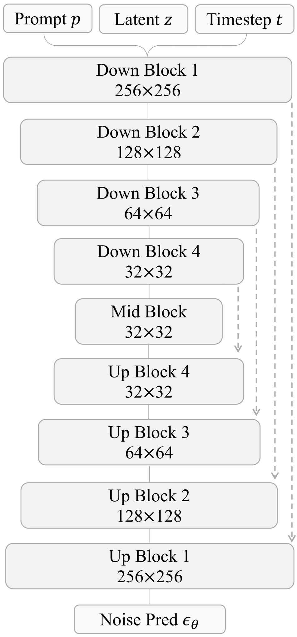
(a)

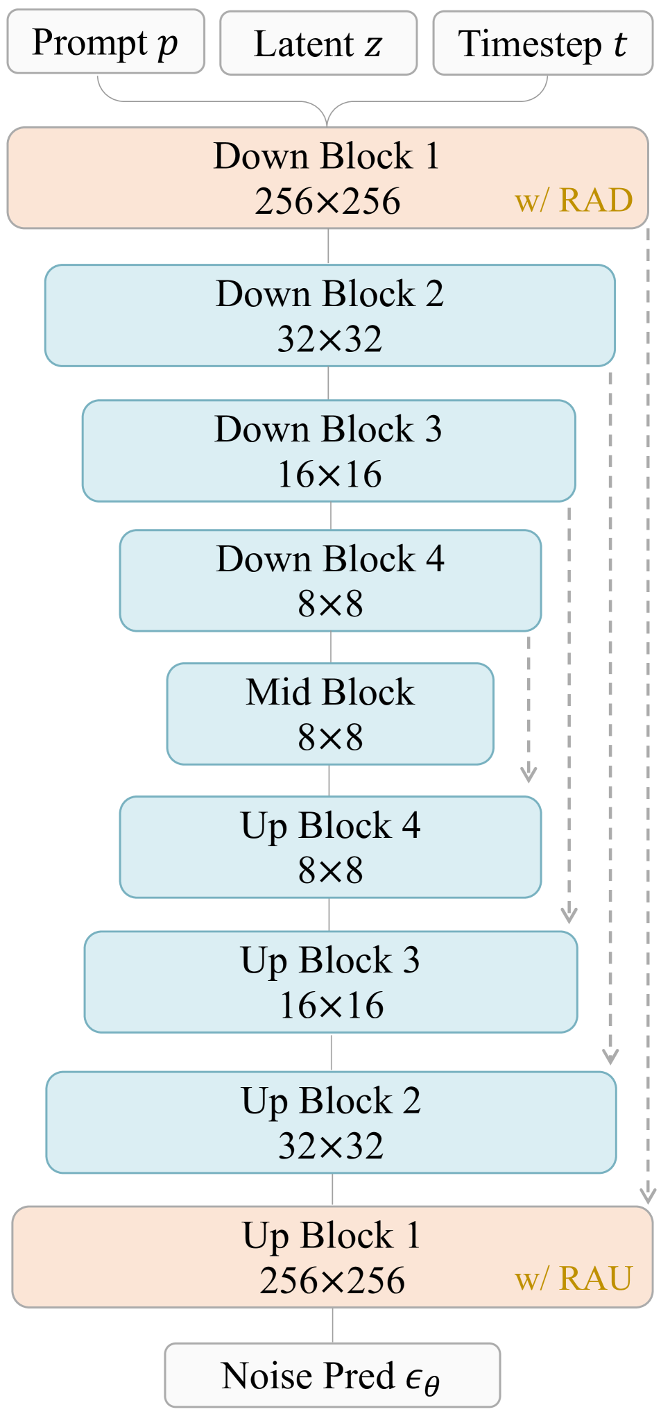
(b)

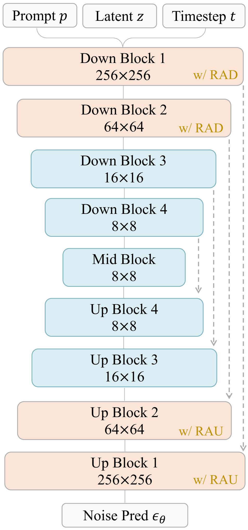
(c)

Figure 18: U-Net variants of SD 1.5 and SD 2.1. (a) Vanilla U-Net. (b) RAU-Net. (c) Progressive RAU-Net. (b) can generate images with 2048$\times$2048 resolution by simply setting $\alpha=\beta=8$, $d=4$, $p=4$. However, a sharp change in resolution caused by interpolation may bring blurriness. We adopt (c), a progressive approach by incorporating RAU and RAD with $\alpha=\beta=4$, $d=2$, $p=2$ into Block 1 and Block 2 to allow the feature map to gradually match the receptive field of the convolution. This progressive method can mitigate blurriness and generate high-quality images.

(a)

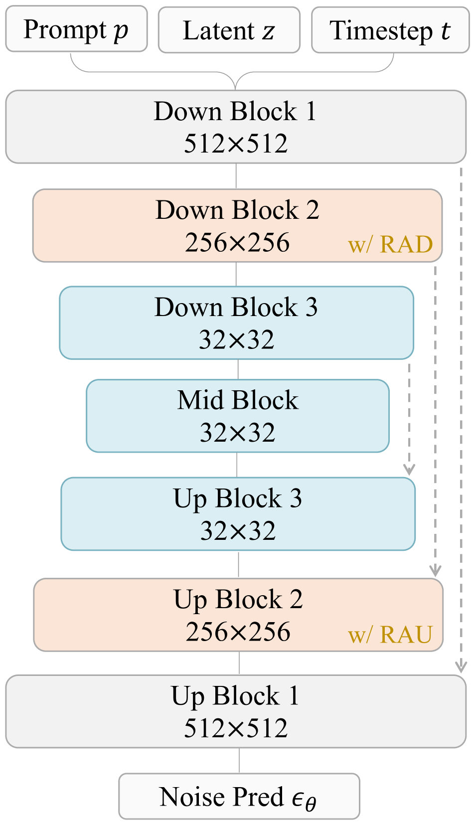
(b)

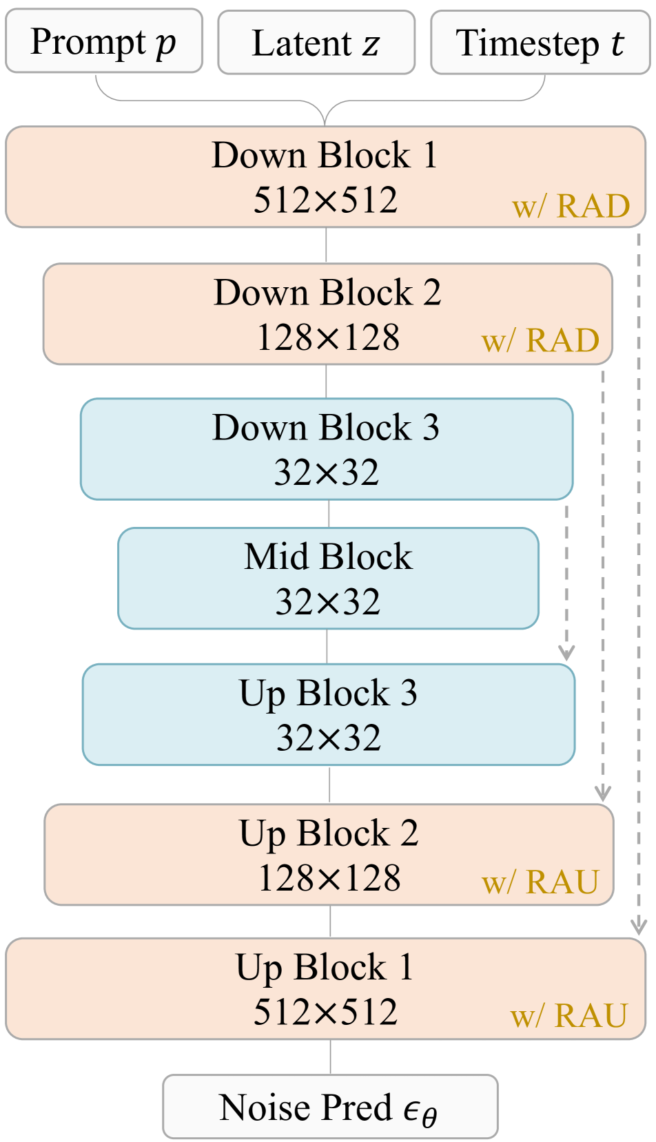
(c)

Figure 19: U-Net variants of SDXL. (a) Vanilla U-Net. (b) RAU-Net. (c) Progressive RAU-Net. The parameter settings of (c) are same with Fig. 20.

As described in the main paper, matching the feature map size with the receptive field of the convolution can generate coherent object structures while potentially affecting image details. Therefore, we choose to gradually reduce the usage of resolution-aware samplers throughout the denoising process for finer image detail when generating images with extreme resolution. Specifically, we employ Progressive RAU-Net in the early stage, followed by RAU-Net in the middle stage, and finally vanilla U-Net in the later stage. We establish two thresholds $T_{1}$ and $T_{2}$: when denoising steps $t<T_{1}$, We use progressive RAU-Net; when $T_{1}\leq t\leq T_{2}$, We use RAU-Net ; when $t>T_{2}$, vanilla U-Net is used. We present the framework in Fig. 17 and generated samples in Fig. 20(b). In the experiment of the main paper, We set $T_{1}=15$ and $T_{2}=35$ for 50 DDIM steps. We incorporate MSW-MSA into Block 1 for SD 1.5 and SD 2.1, and into Block 2 for SDXL. We set the window size as $(128,128)$. The predefined set of shift strides is $\{(0,0),(32,32),(64,64),(96,96)\}$. The classifier-free guidance scales of SD 1.5, SD 2.1, and SDXL are all 7.5.

Appendix D Ablations on resolution-aware operation

In the main paper, for the 1024$\times$1024 resolution generation, RAD is achieved by adjusting the convolution stride and utilizing dilation to enlarge the kernel size. This method downsamples the feature map by a factor of four to accommodate the receptive field of the convolution. Alternatively, a more intuitive approach would be to keep the convolution unchanged and downsample the feature map by a factor of 2 using a pooling operation, which can be written as:

$$\mathcal{RAD}(x,4)=\mathcal{C}_{3,1,2,1}(pool(x,2)).$$ (10)

This method can also achieve the goal of resolution-aware downsampling. In this section, we investigate which methods can generate higher-quality images. We present quantitative comparison in Tab. 8. Compared with the additional pooling operation, the dilation method exhibits superior performance in both FID and CLIP-Score.

(a)

(b)

Figure 20: 2048$\times$2048 resolution samples generated by (a) Directly set $\alpha=8$ in Block 1 of RAU-Net. (b) The final progressive method. The diffusion model version is SD 1.5.

Method	FID$\downarrow$	CLIP-Score$\uparrow$
Pool	26.85	0.304
Dilation	21.81	0.307

Table 8: Quantitative evaluation of two variants of resolution-aware operation on ImageNet [37]. The resolution is 1024$\times$1024 and the diffusion model version SD 1.5.

Appendix E Ablations on window shift

In the main paper, we introduce a window shift strategy that randomly selects a stride from a fixed set of shift strides. In this section, we compare our method with another window shift strategy: Apply window attention and shifted window attention at adjacent timestep. Compared with the window shift strategy in the main paper, This method can mitigate randomness. As shown in Tab. 9, the method proposed in the main paper is comparable with the alternating method. We believe that as long as window connection can be introduced, the differences between different methods are negligible. In practice, any suitable window interaction method for the diffusion model can be selected to efficiently generate images.

Method	FID$\downarrow$	CLIP-Score$\uparrow$
Alternating	21.91	0.306
Ours	21.81	0.307

Table 9: Quantitative evaluation of different window shift strategies on ImageNet. The resolution is 1024$\times$1024 and the diffusion model version is SD 1.5.

Appendix F Additional qualitative results

We provide additional qualitative results, including the comparison between ToMeSD and our MSW-MSA (Fig. 21); visual samples in ablation study (Figs. 22, 23 and 24); comparison between vanilla Stable Diffusion, MultiDiffusion, and our HiDiffusion (Fig. 25); comparison between LDM-SR and HiDiffusion (Figs. 26 and 27); high-resolution samples with various aspect ratios generated by HiDiffusion (Figs. 28, 29, 30, 31, 32, 33, 34 and 35).

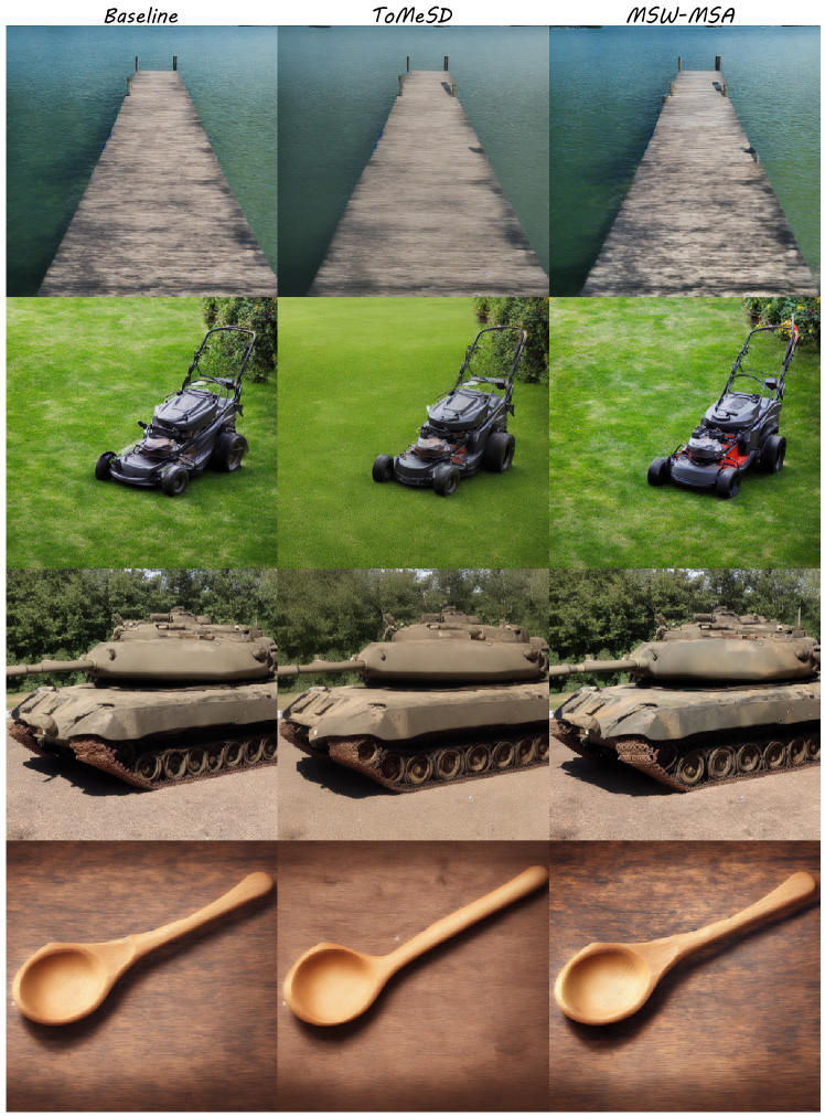
Figure 21: Comparison of 1024$\times$1024 resolution between baseline (SD 1.5 + HiDiffusion without MSW-MSA), ToMeSD and our MSW-MSA on ImageNet. The merge ratio of ToMeSD is 0.5. ToMeSD compromises the fine details of the images. Conversely, our approach is capable of generating results comparable to the baseline.

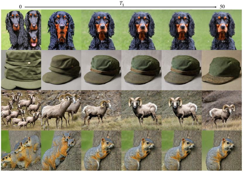
Figure 22: Visual samples with 1024$\times$1024 resolution of different $T_{1}$ on ImageNet. $T_{1}$ ranging from 20 to 40 can effectively mitigate object duplication and maintains high image quality, with $T_{1}$ = 20 yielding the optimal performance.

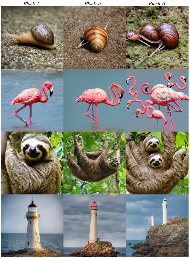
Figure 23: Comparison of 1024$\times$1024 resolution between different locations of Resolution-aware sampler on ImageNet. It can be easily seen that incorporating RAD and RAU in Block 1 can better mitigate object duplication.

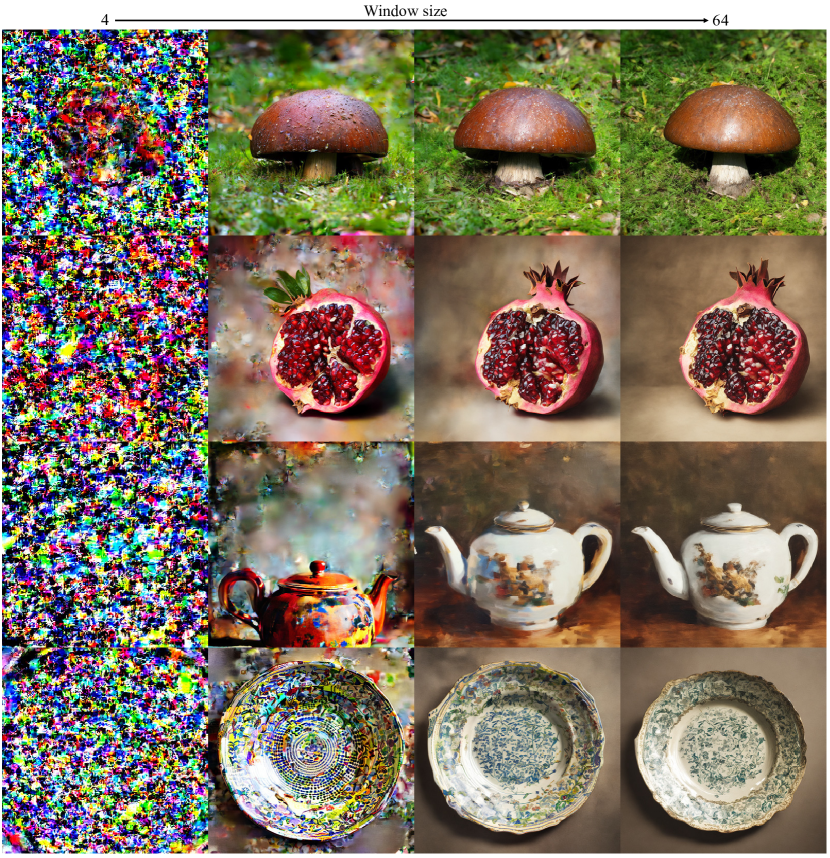
Figure 24: Comparison of 1024$\times$1024 resolution from small window size proposed in Swin Transformer [22] to our proposed large window size on ImageNet. The image quality improves as the window size increases. We achieve the optimal balance between efficiency and performance when the window size is half the height and width of the feature map.

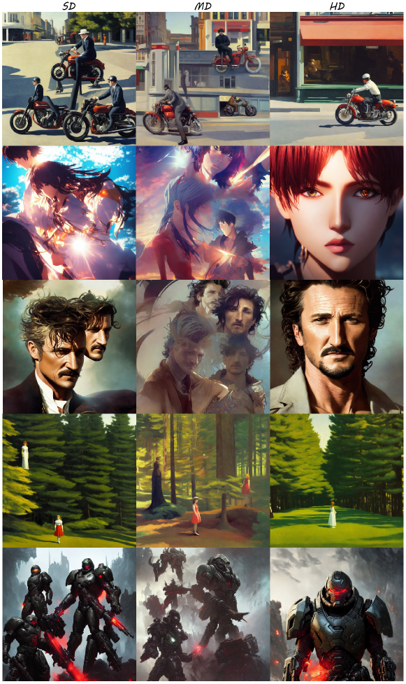
Figure 25: Images with 1024$\times$1024 resolution generated by SD, Multidiffusion (MD) and our HiDiffusion (HD).

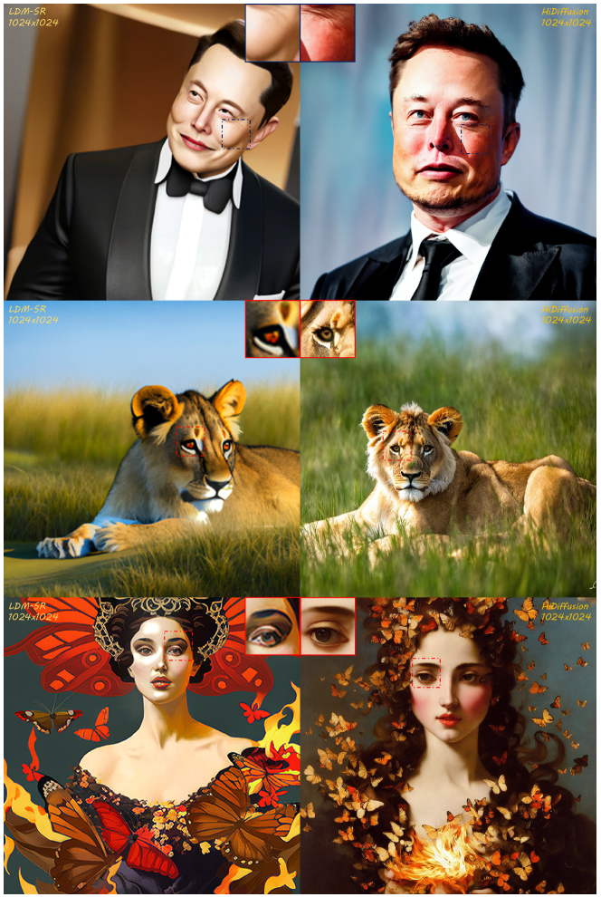
Figure 26: Comparison between LDM-SR and our HiDiffusion. Our HiDiffusion can generate images with higher richness and fine-grained details on 1024$\times$1024 resolution. Best viewed when zoomed in.

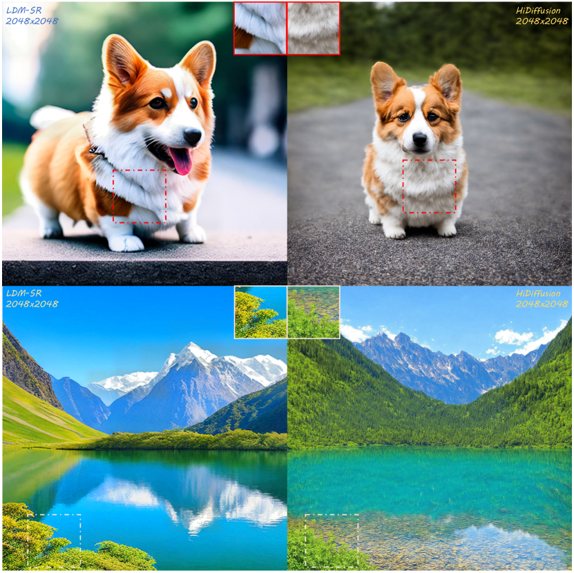
Figure 27: Comparison between LDM-SR and our HiDiffusion. Our HiDiffusion can generate images with higher richness and fine-grained details on 2048$\times$2048 resolution. Best viewed when zoomed in.

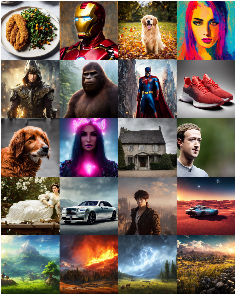
Figure 28: 1024$\times$1024 resolution samples generated by HiDiffusion based on SD 1.5. Best viewed when zoomed in.

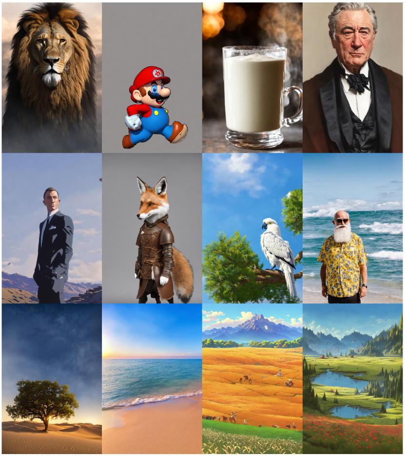
Figure 29: 1536$\times$1024 resolution samples generated by HiDiffusion based on SD 2.1. Best viewed when zoomed in.

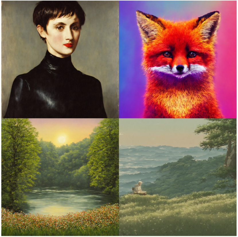
Figure 30: 2048$\times$2048 resolution samples generated by HiDiffusion based on SD 1.5. Best viewed when zoomed in.

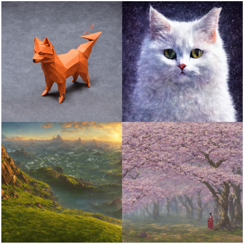
Figure 31: 2048$\times$2048 resolution samples generated by HiDiffusion based on SD 2.1. Best viewed when zoomed in.

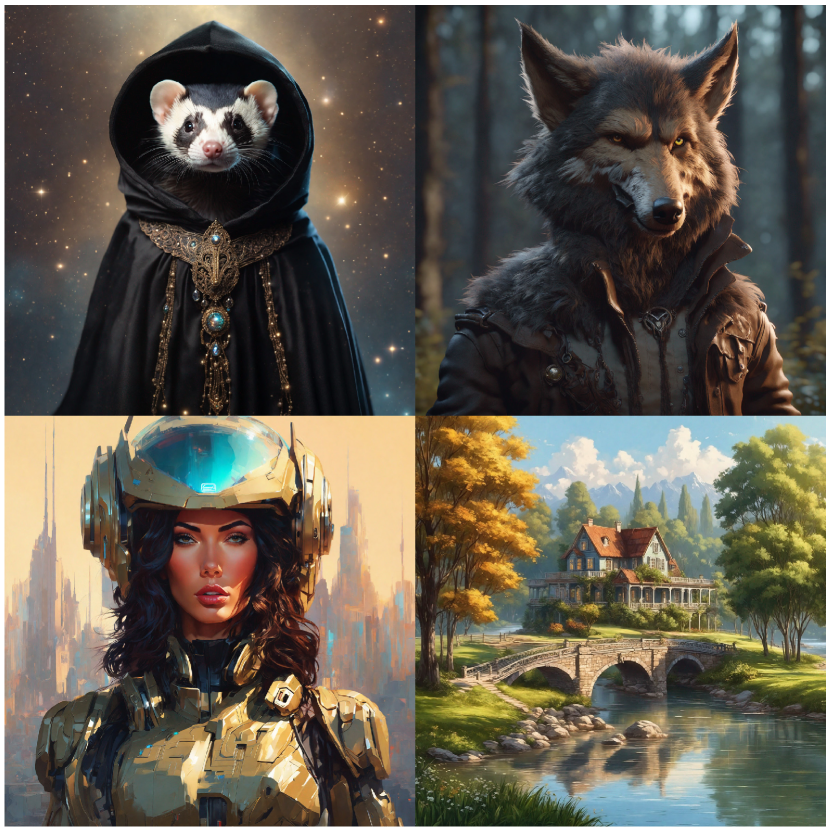
Figure 32: 2048$\times$2048 resolution samples generated by HiDiffusion based on SDXL. Best viewed when zoomed in.

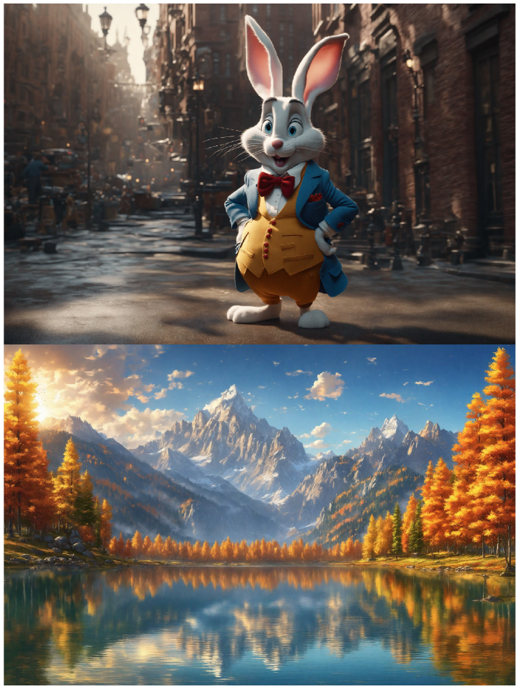
Figure 33: 2048$\times$3072 resolution samples generated by HiDiffusion based on SDXL. Best viewed when zoomed in.

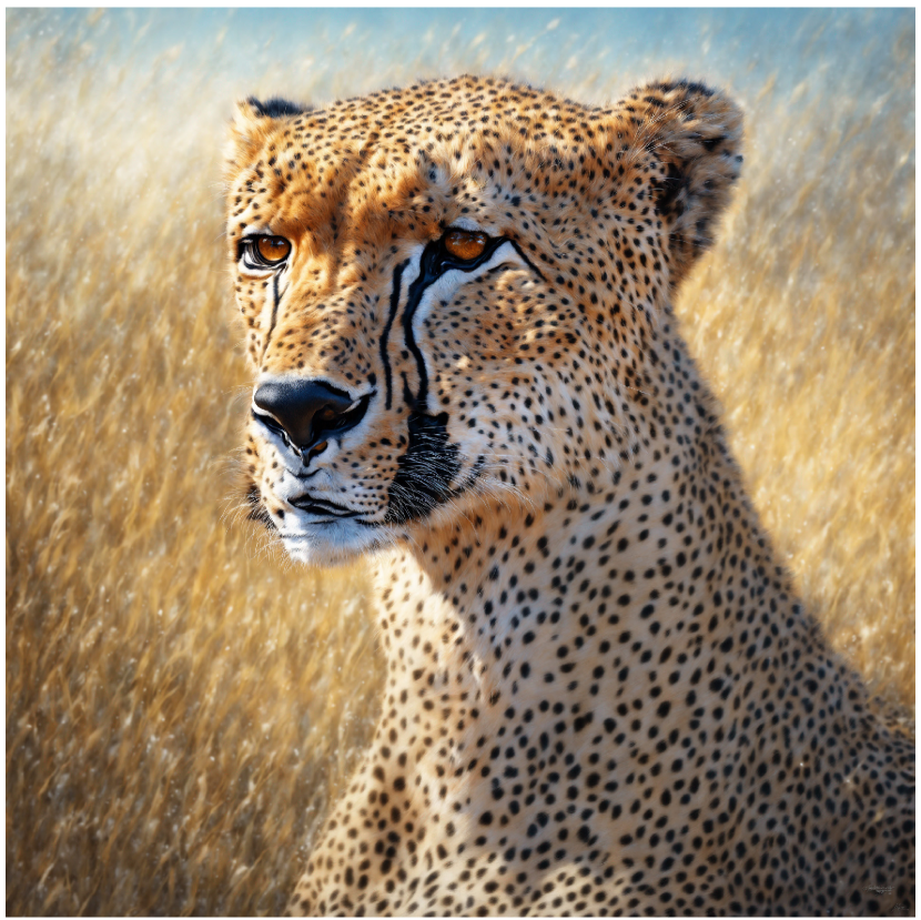
Figure 34: 4096$\times$4096 resolution samples generated by HiDiffusion based on SDXL. Best viewed when zoomed in.

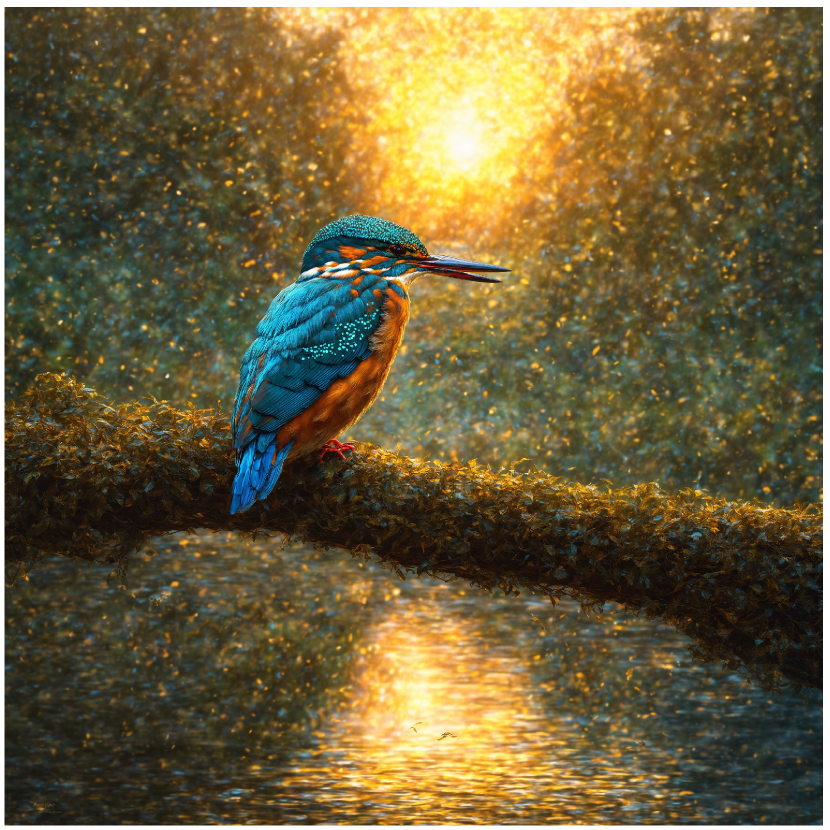
Figure 35: 4096$\times$4096 resolution samples generated by HiDiffusion based on SDXL. Best viewed when zoomed in.

References

- [1] Omer Bar-Tal, Lior Yariv, Yaron Lipman, and Tali Dekel. Multidiffusion: Fusing diffusion paths for controlled image generation. In ICML, 2023.
- [2] Daniel Bolya and Judy Hoffman. Token merging for fast stable diffusion. In CVPRW, pages 4598–4602, 2023.
- [3] Huiwen Chang, Han Zhang, Jarred Barber, AJ Maschinot, Jose Lezama, Lu Jiang, Ming-Hsuan Yang, Kevin Murphy, William T Freeman, Michael Rubinstein, et al. Muse: Text-to-image generation via masked generative transformers. arXiv preprint arXiv:2301.00704, 2023.
- [4] Yu-Hui Chen, Raman Sarokin, Juhyun Lee, Jiuqiang Tang, Chuo-Ling Chang, Andrei Kulik, and Matthias Grundmann. Speed is all you need: On-device acceleration of large diffusion models via gpu-aware optimizations. In CVPR, pages 4650–4654, 2023.
- [5] Prafulla Dhariwal and Alexander Nichol. Diffusion models beat gans on image synthesis. volume 34, pages 8780–8794, 2021.
- [6] Alexey Dosovitskiy, Lucas Beyer, Alexander Kolesnikov, Dirk Weissenborn, Xiaohua Zhai, Thomas Unterthiner, Mostafa Dehghani, Matthias Minderer, Georg Heigold, Sylvain Gelly, et al. An image is worth 16x16 words: Transformers for image recognition at scale. In ICLR, 2021.
- [7] Ian Goodfellow, Jean Pouget-Abadie, Mehdi Mirza, Bing Xu, David Warde-Farley, Sherjil Ozair, Aaron Courville, and Yoshua Bengio. Generative adversarial nets. volume 27, 2014.
- [8] Kaiming He, Xiangyu Zhang, Shaoqing Ren, and Jian Sun. Deep residual learning for image recognition. In CVPR, pages 770–778, 2016.
- [9] Martin Heusel, Hubert Ramsauer, Thomas Unterthiner, Bernhard Nessler, and Sepp Hochreiter. Gans trained by a two time-scale update rule converge to a local nash equilibrium. In NeurIPS, 2017.
- [10] Jonathan Ho, Ajay Jain, and Pieter Abbeel. Denoising diffusion probabilistic models. In NeurIPS, pages 6840–6851, 2020.
- [11] Jonathan Ho, Chitwan Saharia, William Chan, David J Fleet, Mohammad Norouzi, and Tim Salimans. Cascaded diffusion models for high fidelity image generation. The Journal of Machine Learning Research, 23(1):2249–2281, 2022.
- [12] Emiel Hoogeboom, Jonathan Heek, and Tim Salimans. simple diffusion: End-to-end diffusion for high resolution images. arXiv preprint arXiv:2301.11093, 2023.
- [13] Ramesh Jain, Rangachar Kasturi, Brian G Schunck, et al. Machine vision, volume 5. McGraw-hill New York, 1995.
- [14] Álvaro Barbero Jiménez. Mixture of diffusers for scene composition and high resolution image generation. arXiv preprint arXiv:2302.02412, 2023.
- [15] Zhiyu Jin, Xuli Shen, Bin Li, and Xiangyang Xue. Training-free diffusion model adaptation for variable-sized text-to-image synthesis. arXiv preprint arXiv:2306.08645, 2023.
- [16] Tero Karras, Samuli Laine, Miika Aittala, Janne Hellsten, Jaakko Lehtinen, and Timo Aila. Analyzing and improving the image quality of stylegan. In CVPR, pages 8110–8119, 2020.
- [17] Yuseung Lee, Kunho Kim, Hyunjin Kim, and Minhyuk Sung. Syncdiffusion: Coherent montage via synchronized joint diffusions. In NeurIPS, 2023.
- [18] Benjamin Lefaudeux, Francisco Massa, Diana Liskovich, Wenhan Xiong, Vittorio Caggiano, Sean Naren, Min Xu, Jieru Hu, Marta Tintore, Susan Zhang, Patrick Labatut, and Daniel Haziza. xformers: A modular and hackable transformer modelling library. https://github.com/facebookresearch/xformers, 2022.
- [19] Lijiang Li, Huixia Li, Xiawu Zheng, Jie Wu, Xuefeng Xiao, Rui Wang, Min Zheng, Xin Pan, Fei Chao, and Rongrong Ji. Autodiffusion: Training-free optimization of time steps and architectures for automated diffusion model acceleration. pages 7105–7114, 2023.
- [20] Wentong Liao, Kai Hu, Michael Ying Yang, and Bodo Rosenhahn. Text to image generation with semantic-spatial aware gan. In CVPR, pages 18187–18196, 2022.
- [21] Tsung-Yi Lin, Michael Maire, Serge Belongie, James Hays, Pietro Perona, Deva Ramanan, Piotr Dollár, and C Lawrence Zitnick. Microsoft coco: Common objects in context. In ECCV, pages 740–755, 2014.
- [22] Ze Liu, Yutong Lin, Yue Cao, Han Hu, Yixuan Wei, Zheng Zhang, Stephen Lin, and Baining Guo. Swin transformer: Hierarchical vision transformer using shifted windows. In ICCV, pages 10012–10022, 2021.
- [23] Cheng Lu, Yuhao Zhou, Fan Bao, Jianfei Chen, Chongxuan Li, and Jun Zhu. Dpm-solver: A fast ode solver for diffusion probabilistic model sampling in around 10 steps. In NeurIPS, pages 5775–5787, 2022.
- [24] Cheng Lu, Yuhao Zhou, Fan Bao, Jianfei Chen, Chongxuan Li, and Jun Zhu. Dpm-solver++: Fast solver for guided sampling of diffusion probabilistic models. arXiv preprint arXiv:2211.01095, 2022.
- [25] Chenlin Meng, Robin Rombach, Ruiqi Gao, Diederik Kingma, Stefano Ermon, Jonathan Ho, and Tim Salimans. On distillation of guided diffusion models. In CVPR, pages 14297–14306, 2023.
- [26] Alex Nichol, Prafulla Dhariwal, Aditya Ramesh, Pranav Shyam, Pamela Mishkin, Bob McGrew, Ilya Sutskever, and Mark Chen. Glide: Towards photorealistic image generation and editing with text-guided diffusion models. arXiv preprint arXiv:2112.10741, 2021.
- [27] Xuran Pan, Tianzhu Ye, Zhuofan Xia, Shiji Song, and Gao Huang. Slide-transformer: Hierarchical vision transformer with local self-attention. In CVPR, pages 2082–2091, 2023.
- [28] Zhihong Pan, Riccardo Gherardi, Xiufeng Xie, and Stephen Huang. Effective real image editing with accelerated iterative diffusion inversion. In ICCV, pages 15912–15921, 2023.
- [29] Dustin Podell, Zion English, Kyle Lacey, Andreas Blattmann, Tim Dockhorn, Jonas Müller, Joe Penna, and Robin Rombach. Sdxl: Improving latent diffusion models for high-resolution image synthesis. arXiv preprint arXiv:2307.01952, 2023.
- [30] Alec Radford, Jong Wook Kim, Chris Hallacy, Aditya Ramesh, Gabriel Goh, Sandhini Agarwal, Girish Sastry, Amanda Askell, Pamela Mishkin, Jack Clark, et al. Learning transferable visual models from natural language supervision. In ICML, pages 8748–8763. PMLR, 2021.
- [31] Aditya Ramesh, Prafulla Dhariwal, Alex Nichol, Casey Chu, and Mark Chen. Hierarchical text-conditional image generation with clip latents. arXiv preprint arXiv:2204.06125, 1(2):3, 2022.
- [32] Aditya Ramesh, Mikhail Pavlov, Gabriel Goh, Scott Gray, Chelsea Voss, Alec Radford, Mark Chen, and Ilya Sutskever. Zero-shot text-to-image generation. In ICML, pages 8821–8831. PMLR, 2021.
- [33] Scott Reed, Zeynep Akata, Xinchen Yan, Lajanugen Logeswaran, Bernt Schiele, and Honglak Lee. Generative adversarial text to image synthesis. In ICML, pages 1060–1069. PMLR, 2016.
- [34] Robin Rombach, Andreas Blattmann, Dominik Lorenz, Patrick Esser, and Björn Ommer. High-resolution image synthesis with latent diffusion models. In CVPR, pages 10684–10695, 2022.
- [35] Olaf Ronneberger, Philipp Fischer, and Thomas Brox. U-net: Convolutional networks for biomedical image segmentation. In MICCAI, pages 234–241. Springer, 2015.
- [36] Nataniel Ruiz, Yuanzhen Li, Varun Jampani, Yael Pritch, Michael Rubinstein, and Kfir Aberman. Dreambooth: Fine tuning text-to-image diffusion models for subject-driven generation. In CVPR, pages 22500–22510, 2023.
- [37] Olga Russakovsky, Jia Deng, Hao Su, Jonathan Krause, Sanjeev Satheesh, Sean Ma, Zhiheng Huang, Andrej Karpathy, Aditya Khosla, Michael Bernstein, et al. Imagenet large scale visual recognition challenge. IJCV, 115:211–252, 2015.
- [38] Chitwan Saharia, William Chan, Saurabh Saxena, Lala Li, Jay Whang, Emily Denton, Seyed Kamyar Seyed Ghasemipour, Burcu Karagol Ayan, S Sara Mahdavi, Rapha Gontijo Lopes, et al. Photorealistic text-to-image diffusion models with deep language understanding. arXiv preprint arXiv:2205.11487, 2022.
- [39] Tim Salimans and Jonathan Ho. Progressive distillation for fast sampling of diffusion models. arXiv preprint arXiv:2202.00512, 2022.
- [40] Christoph Schuhmann, Romain Beaumont, Richard Vencu, Cade Gordon, Ross Wightman, Mehdi Cherti, Theo Coombes, Aarush Katta, Clayton Mullis, Mitchell Wortsman, et al. Laion-5b: An open large-scale dataset for training next generation image-text models. In NeurIPS, pages 25278–25294, 2022.
- [41] Jiaming Song, Chenlin Meng, and Stefano Ermon. Denoising diffusion implicit models. In ICLR, 2021.
- [42] Yang Song and Stefano Ermon. Generative modeling by estimating gradients of the data distribution. In NeurIPS, pages 11895–11907, 2019.
- [43] Yang Song, Jascha Sohl-Dickstein, Diederik P Kingma, Abhishek Kumar, Stefano Ermon, and Ben Poole. Score-based generative modeling through stochastic differential equations. In ICLR, 2021.
- [44] Jiayan Teng, Wendi Zheng, Ming Ding, Wenyi Hong, Jianqiao Wangni, Zhuoyi Yang, and Jie Tang. Relay diffusion: Unifying diffusion process across resolutions for image synthesis. arXiv preprint arXiv:2309.03350, 2023.
- [45] Enze Xie, Lewei Yao, Han Shi, Zhili Liu, Daquan Zhou, Zhaoqiang Liu, Jiawei Li, and Zhenguo Li. Difffit: Unlocking transferability of large diffusion models via simple parameter-efficient fine-tuning. arXiv preprint arXiv:2304.06648, 2023.
- [46] Tao Xu, Pengchuan Zhang, Qiuyuan Huang, Han Zhang, Zhe Gan, Xiaolei Huang, and Xiaodong He. Attngan: Fine-grained text to image generation with attentional generative adversarial networks. In CVPR, pages 1316–1324, 2018.
- [47] Xingyi Yang, Daquan Zhou, Jiashi Feng, and Xinchao Wang. Diffusion probabilistic model made slim. In CVPR, pages 22552–22562, 2023.
- [48] Fisher Yu and Vladlen Koltun. Multi-scale context aggregation by dilated convolutions. arXiv preprint arXiv:1511.07122, 2015.
- [49] Chenshuang Zhang, Chaoning Zhang, Mengchun Zhang, and In So Kweon. Text-to-image diffusion model in generative ai: A survey. arXiv preprint arXiv:2303.07909, 2023.
- [50] Qingping Zheng, Yuanfan Guo, Jiankang Deng, Jianhua Han, Ying Li, Songcen Xu, and Hang Xu. Any-size-diffusion: Toward efficient text-driven synthesis for any-size hd images. arXiv preprint arXiv:2308.16582, 2023.