Improving Stability during Upsampling – on the Importance of Spatial Context

Abstract

State-of-the-art models for pixel-wise prediction tasks such as image restoration, image segmentation, or disparity estimation, involve several stages of data resampling, in which the resolution of feature maps is first reduced to aggregate information and then sequentially increased to generate a high-resolution output. Several previous works have investigated the effect of artifacts that are invoked during downsampling and diverse cures have been proposed that facilitate to improve prediction stability and even robustness for image classification. However, equally relevant, artifacts that arise during upsampling have been less discussed. This is significantly relevant as upsampling and downsampling approaches face fundamentally different challenges. While during downsampling, aliases and artifacts can be reduced by blurring feature maps, the emergence of fine details is crucial during upsampling. Blurring is therefore not an option and dedicated operations need to be considered. In this work, we are the first to explore the relevance of context during upsampling by employing convolutional upsampling operations with increasing kernel size while keeping the encoder unchanged. We find that increased kernel sizes can in general improve the prediction stability in tasks such as image restoration or image segmentation, while a block that allows for a combination of small-size kernels for fine details and large-size kernels for artifact removal and increased context yields the best results.

1 Introduction

subBaseline
Improved (ours)
		clean - within domain	attacked

Figure 1: Deblurring results on the GoPro dataset [53] using the state-of-the-art NAFNet [13] on in-domain data (left) and under 5-step PGD attack (right). The proposed modification of increasing context during training(bottom row) is simple and increases the stability of the model during upsampling significantly.

Deep neural networks (DNNs) typically aggregate image information through operations such as convolution or attention and spatial downsampling (e.g. striding) of feature maps. Deep models can thus encode information and dependencies from large receptive fields even when only small convolutional filters are used [30, 35, 36, 59, 70]. Yet, the advantage of encoding a larger spatial context within convolutional network layers has recently been leveraged e.g. in [44, 14, 43], to facilitate results on par with or better than recent vision transformers [59, 72, 74] that encode spatially distant context via self-attention. In another line of research, larger convolution filters have been linked to a model’s favorable spectral properties and robustness, e.g. [67, 48, 26, 25, 24, 80, 84, 34]. Interestingly, maybe due to the prevalence of image classification tasks in the context of model robustness[33, 65, 21, jung2023neural], most previous works on feature map resampling and model stability focus on image encoding.

However, we find that both aspects, the aggregation of context and the removal of sampling artifacts, are equally important for image decoding, i.e. in the context of pixel-wise prediction tasks such as image restoration [78], semantic segmentation [60, 6, 28], optical flow estimation [18, 37, 73] and disparity estimation [42, 5, 8]. Analogous to performing downsampling by using convolution [79], naïve upsampling can introduce artifacts in the feature representation, such as grid artifacts [55, 3] or ringing artifacts [52]. By attacking the networks with white-box adversarial attacks [23, 41, 27], we provide empirical indicators that such spectral artifacts during upsampling are highly relevant for model robustness. Our results further show that increased upsampling context and decreased spectral artifacts have a favorable effect on model robustness, see Figure 1 for an example. Specifically, our work is driven by the following hypotheses:

Hypothesis 1 (H1):

Large kernels in transposed convolution operations provide more context and reduce spectral artifacts and can therefore be leveraged by the network to facilitate better and more robust pixel-wise predictions.

Hypothesis 2 (H2):

To leverage prediction context and reduce spectral artifacts, it is crucial to increase the size of transposed convolution kernels. Increasing the size of normal (i.e. non-upsampling) decoder convolutions does not have this effect.

While our work focuses on the analysis of the described hypotheses H1 and H2, the resulting design choices facilitate improvements on recent model architectures, for example for image restoration [78] or disparity estimation [42]. The main contributions of our work are as follows:

• We investigate larger convolution kernel sizes in transposed convolutions for upsampling in diverse models for pixel-wise prediction tasks. We find that using large kernels indeed helps the performance. However, using small and large kernels in parallel provides the best overall results.

• We show that better upsampling can improve networks’ generalization ability and robustness by reducing spectral artifacts.

• We provide empirical evidence for our findings on diverse architectures (including vision transformer-based architectures) and downstream tasks such as image restoration and depth estimation.

2 Related Work

In the following, we will discuss recent challenges for neural networks regarding artifacts introduced by spatial sampling methods  [55, 3, 52]. Further, we review related work on the most recent use of large kernels in CNNs. Finally, we provide an overview of adversarial attacks to evaluate the overall robustness of a trained network.

Spectral Artifacts.

Several prior works have studied the effect of downsampling operations on model robustness , e.g. [39, 34, 26, 24, 80, 84]. Inspired by [26], [24] propose for example aliasing-free downsampling in the frequency domain which translates to an infinitely large blurring filter before downsampling in the spatial domain. Thus, for image classification, using large filter kernels has been shown to remove artifacts from downsampled representations and it leads to favorable robustness in all these cases [39, 34, 26]. However, all these works focus on improving the properties of encoder networks.

Models that use transposed convolutions their decoders are widely used for tasks like image generation [22, 58] or segmentation [45, 54, 60, 6]. However, in simple transposed convolutions, the convolution kernels overlap based on the chosen stride and kernel size. If the stride is smaller than the kernel size, this will cause overlaps in the operation, leading to uneven contributions to different pixels in the upsampled feature map and thus to grid-like artifacts [3, 55]. Further, image resampling can lead to aliases that become visible as ringing artifacts [67]. In the context of deepFake detection, image generation, and deblurring, several works analyzed [16, 11, 40, 31, 38] and improved upsampling techniques [39, 20, 76, 69] to reduce visual artifacts.

Some architectures like PSPNet [82], PSANet [83], or PSMNet [12] simply use interpolation operations for upsampling the feature representations. While this reduces grid artifacts as interpolation smoothens out the feature maps, it also has major drawbacks: The interpolation leads to overly smooth predictions, in particular, apparent in the PSPNet segmentation masks. The segmentation masks over-smoothen around edges and often miss out on thin details (predictions showing these are included in the Sec. B.3.1). This observation already shows why image encoding and decoding have to be considered separately when it comes to sampling artifacts. While during encoding, artifacts can be reduced by blurring, the main purpose of decoder networks is to reduce blur in many applications, in order to create fine-granular, pixel-wise accurate outputs. This paper is the first to investigate the significance of upsampling filter sizes for prediction stability under data perturbations.

Large Kernels.

For image classification, [44] showed that using large kernels like 7$\times$7 in the CNN convolution layer can outperform self-attention based vision transformers [59, 72, 74]. In [28, 14, 43, 56], the receptive field of the convolution operations was further expanded by using larger kernels, up to 31$\times$31 and 51$\times$51. These larger receptive fields provide more context to the encoder, leading to better performance on classification, segmentation, or object detection tasks. [14, 43] use a small kernel in parallel to capture the local context as well as more global context. In contrast to these works, we investigate if larger kernels can benefit upsampling when considering pixel-wise prediction tasks such as image restoration or segmentation.

Adversarial Attacks.

The purpose of adversarial attacks is to reveal neural networks’ weaknesses [26, 71, 2, 63] by perturbing pixel values in the input image [23, 9, 41]. These perturbations should lead to a false prediction even though the changes are hardly visible [23, 51, 71]. Especially attacks that have access to the network’s architecture and weights, so-called white-box attacks, are a common approach to analyzing weaknesses within the networks’ structure [9, 23]. They employ the gradient of the network to optimize the perturbation, which is bounded within an $\epsilon$-ball of the original image, i.e. $\epsilon$ defines the strength of the attack. Most adversarial attacks are proposed to attack classification networks like the one-step Fast Gradient Sign Method (FGSM) [23] or the multi-step Projected Gradient Descent (PGD) attack [41].

However, they can be adapted to other tasks as e.g. in [57, 77, 49]. Furthermore, there are dedicated methods like SegPGD [27] for attacks on semantic segmentation models or PCFA [63] and [64, 61] for optical flow models and CosPGD [2] and others [62] for other pixel-wise prediction tasks. We evaluate model stability considering adversarial attacks such as PGD and CosPGD for image restoration and FGSM and SegPGD for semantic segmentation.

3 Spectral and Grid Artifacts

In the following, we theoretically review artifacts that are caused during upsampling. We start by describing spectral artifacts [67], similar to the discussion in [16].

Consider, w.l.o.g., a one-dimensional signal $I$ and its discrete Fourier Transform $\mathcal{F}({I})$ with $k$ being the index of discrete frequencies

$$\mathcal{F}({I})_{k}=\sum_{j=0}^{N-1}e^{-2\pi i\cdot\frac{jk}{N}}\cdot I_{j},\quad\mathrm{for}\quad k=0,\dots,N-1.$$

During decoding, we need to upsample the spatial resolution of $I$ to get $I^{\mathrm{up}}$. For example for upsampling factor $2$, which can be considered a standard case, we have for $\bar{k}=0,\dots,2N-1$

$$\mathcal{F}(I)^{\mathrm{up}}_{\bar{k}} =\sum_{j=0}^{2N-1}e^{-2\pi i\cdot\frac{j\bar{k}}{2\cdot N}}\cdot I^{\mathrm{up}}_{j}$$

$$=\sum_{j=0}^{N-1}e^{-2\pi i\cdot\frac{2\cdot j\bar{k}}{2\cdot N}}I_{j}+\sum_{j=0}^{N-1}e^{-2\pi i\cdot\frac{2\cdot(j+1)\bar{k}}{2\cdot N}}\bar{I}_{j},$$ (1)

where $\bar{I}_{j}=0$ in transposed convolutions [45, 15]. Then, the second term in (1) can be dropped and the first term resembles the original $\mathcal{F}(I)$. Equivalently, we can rewrite Eq. (1) for $\bar{I}_{j}=0$ using a Dirac impulse comb as

$$\eqref{eq:theory2} =\sum_{j=0}^{2N-1}e^{-2\pi i\cdot\frac{j\bar{k}}{2\cdot N}}\cdot\sum_{t=-\infty}^{\infty}I^{\mathrm{up}}_{j}\cdot\delta(j-2t).$$ (2)

If we now apply the pointwise multiplication with the Dirac impulse comb as convolution in the Fourier domain (assuming periodicity) [19], it is

$$\mathcal{F}(I)^{\mathrm{up}}_{\bar{k}} =\frac{1}{2}\cdot\sum_{t=-\infty}^{\infty}\left(\sum_{j=-\infty}^{\infty}e^{-2\pi i\cdot\frac{j\bar{k}}{2N}}I^{\mathrm{up}}_{j}\right)\left(\bar{k}-\frac{t}{2}\right)$$

$$\overset{\eqref{eq:theory2}}{=} \frac{1}{2}\cdot\sum_{t=-\infty}^{\infty}\left(\sum_{j=-\infty}^{\infty}e^{-2\pi i\cdot\frac{j\bar{k}}{N}}\cdot I_{j}\right)\left(\bar{k}-\frac{t}{2}\right).$$ (3)

We can see that such upsampling creates a high-frequency replica of the signal in $\mathcal{F}({I})^{\mathrm{up}}$ and spatial frequencies apparent beyond $\frac{N}{2}$ may be impacted by spectral artifacts [16].

Additionally, in simple transposed convolutions, the convolution kernels may overlap based on the chosen stride and kernel size. If the stride is smaller than the kernel size, this will cause overlaps in the operation, leading to uneven contributions to different pixels in the upsampled feature map and thus to grid-like artifacts [3, 55].

Note that, in Eq. (1), pixel shuffle [68] will set $\bar{I}_{j}$ to completely unrelated values of a different feature map channel, leading to issues similar to those in transposed convolutions. Furthermore, it is $\bar{I}_{j}=\frac{I_{j-1}+I_{j}}{2}$ for bi-linear interpolation. Yet, bi-linear interpolation provides rather smooth results in the upsampled data and is, therefore, less suitable for, for example, image restoration or segmentation tasks, where fine structural details are supposed to emerge in the upsampled data. Therefore, transposed convolutions are often employed despite the mentioned drawbacks. Conveniently, the convolution kernel in transposed convolutions itself can reduce the described artifacts when acting like a blur operator. Sufficiently large kernel sizes that increase spatial context are therefore appropriate to allow for the model to learn when to blur and when to preserve/sharpen results.

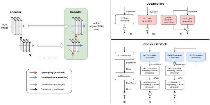
Figure 2: Abstract representation of a UNet-like architecture. While for different tasks, the implementation of the mode encoder varies (including transformer-based encoders), our study focuses on the model decoder (in green). The backbone for the decoder is commonly a ResNet-like structure for feature extraction [60, 6], additionally we also used a ConvNeXt-like [44] structure. In particular, we investigate variants of different upsampling operations for fixed decoder blocks (operations along the red arrows in the decoder). We consider, as probe for H1, the baseline transposed upconvolution ((a) in top right), an increased convolution kernel size ((b) in top right), and an increased convolution kernel with a second path using a small convolution kernel ((c) in the top right). To test whether the plain increase in parameters is responsible for improved results (zero hypothesis, H2), we also ablate on the increase of convolution kernel sizes in the decoder block (operations along the blue arrows in the green block), as shown on the bottom right. We consider the common ResNet-like decoder building block structure (in (d)) and two ConvNext-like structured backbones for the decoder building block in (e) and (f), where (f) has an additional small convolution applied in parallel, analog to (c).

4 Improved Upsampling using Large Kernels

Driven by the observations on upsampling artifacts, we aim to investigate the advantage of larger kernel sizes during upsampling, such as semantic segmentation or disparity estimation. Therefore, we keep the models’ encoder part fixed and exclusively change operations in the architecture of the decoder part of the model. There, we have two design choices: Upsampling – The kernel size for the transposed convolution operations that learn upsampling, and Decoder Block – The kernel size in the convolution operations of blocks that learn to decode the features. Probing options for Upsampling works towards proving H1 while a combination of both options proves H2, i.e. shows that a pure increase in the decoder parameters does not have the desired effect. This is considered in our ablation study in Sec. 5.4.1.

Figure 2 summarizes the studied options for an example of a UNet-like architecture [60]. The model decoder is depicted in the green box. Operations that we consider to be executed along the red upwards arrows (Upsampling Operators) are detailed in the top right part of the figure (operations (a) to (c)). Operations that we consider to be executed along the blue sideways arrows (Decoder Building Blocks) are depicted in the bottom right (operations (d) to (f)).

Model Details

Here, we provide details on the studied models. Implementation details are in the Appendix A.

Transposed Convolution Kernels for Upsampling The upsampling operation is typically performed with small kernels (2$\times$2 or 3$\times$3) in the transposed convolution operations [60, 10, 7]. We aim to increase the spatial context during upsampling and to reduce grid artifacts. Thus we use larger kernels. We either use 7$\times$7 transposed convolutions or 11$\times$11 transposed convolutions with a parallel 3$\times$3 transposed convolution. Adding a parallel 3$\times$3 kernel is motivated by [14], as large convolution kernels tend to lose local context, and thus adding a parallel small kernel helps to overcome this potential drawback (see Sec. B.3).

Decoder Building Blocks To verify that the measurable effects are due to the improved upsampling and not due to merely increasing the decoder capacity, we also ablate on decoder convolution blocks similar to convolution blocks used in the ConvNeXt [44] basic block for encoding. While the standard ConvNeXt block uses a 7$\times$7 depth-wise convolution, we consider 7$\times$7 and 11$\times$11 group-wise convolutions, followed by layers present in a ConvNeXt basic block to analyze the importance of the receptive field within the block. Figure 2 (bottom right e) and f)) shows the structure of a ConvNeXt-style building block used in our work. First, a group-wise convolution is performed, followed by a LayerNorm [4] and two 1$\times$1 convolutions which just like [44] creates an inverted bottleneck by first increasing the channel dimension and after a GELU [32] activation compressing the channel dimension again. We consider the ResNet-style building block (Figure 2, d)), with 3$\times$3 convolution, yet without skip connection, as our baseline when studying this architectural design choice.

	PixelShuffle	$3\times 3$	$7\times 7+3\times 3$ (Ours)	$11\times 11+3\times 3$ (Ours)
subclean
subattacked

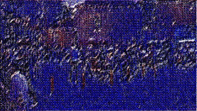
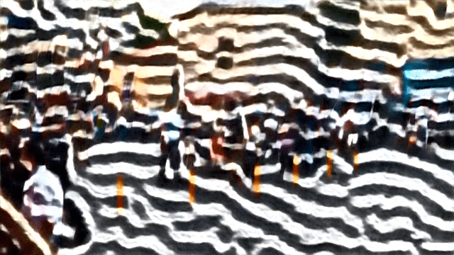
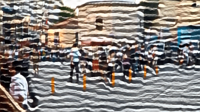
Figure 3: Comparing images reconstructed by all models after 10-step PGD attack with $\epsilon=\frac{8}{255}$ on Restormer [78] and our modified model. Results improve significantly in terms of stability under attack. Examples for different attack budgets are given in the appendix.

	PixelShuffle	$3\times 3$	$7\times 7+3\times 3$ (Ours)	$11\times 11+3\times 3$ (Ours)
subclean
subattacked

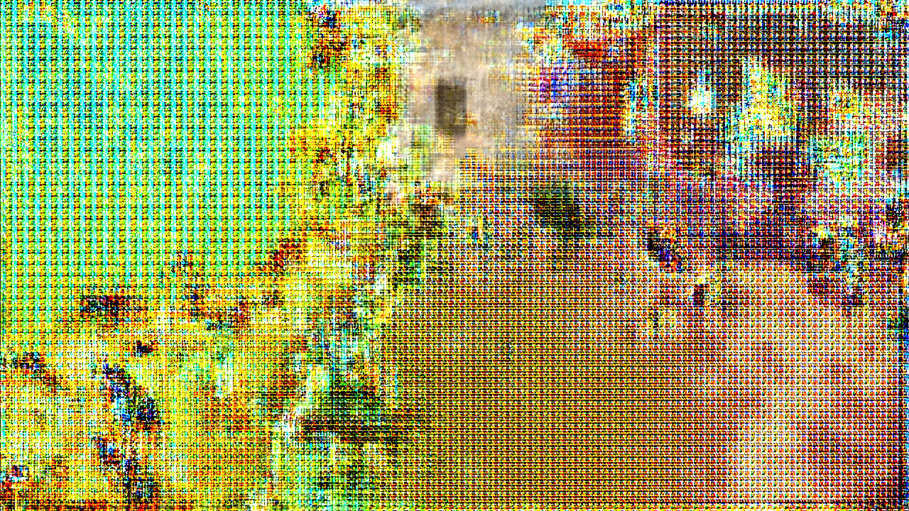
Figure 4: Images reconstructed by NAFNet [13] and our modified model after 10-step PGD attack with $\epsilon=\frac{8}{255}$. Our results improve significantly in terms of stability under attack. More examples for [13] and [78] using different attack budgets are given in the appendix.

5 Experiments

In the following, we evaluate the effect of the considered upsampling operators in several applications. We start by evaluating the effect on the stability of recent SotA image restoration models [78, 13], then provide results on semantic segmentation using more generic convolutional architectures that allow us to provide compulsory ablations. Last, we show that our results also extend to a recently proposed model for disparity estimation [42]. We provide details on the used adversarial attacks, datasets, reported metrics, and other experimental details in Appendix A.

Table 1: Comparison of performances of different upsampling methods in SotA Image Restoration Networks on the GoPro dataset. The architectures use Pixel Shuffle for Upsampling, we propose replacing the Pixel Shuffle with Transposed Convolution operations using the large filter. We report additional results using adversarial training in Tab. 15.

Network	Upsampling Method	Test Accuracy		CosPGD attack iterations						PGD attack iterations
				5		10		20		5		10		20
		PSNR	SSIM	PSNR	SSIM	PSNR	SSIM	PSNR	SSIM	PSNR	SSIM	PSNR	SSIM	PSNR	SSIM
Restormer	Pixel Shuffle	31.99	0.9635	11.36	0.3236	9.05	0.2242	7.59	0.1548	11.41	0.3256	9.04	0.2234	7.58	0.1543
	Transposed Conv 3$\times$3	9.68	0.095	8.24	0.0452	8.53	0.0628	8.44	0.0631	7.66	0.0464	7.72	0.0577	8.64	0.0527
	Transposed Conv 7$\times$7 + 3 $\times$3 (Ours)	29.51	0.9337	13.69	0.4186	11.53	0.3136	10.16	0.2484	13.69	0.4183	11.54	0.3137	10.16	0.2483
	Transposed Conv 11$\times$11 + 3$\times$3 (Ours)	29.44	0.9324	14.65	0.4251	12.83	0.3438	11.48	0.29	14.65	0.4253	12.84	0.3445	11.48	0.2893
NAFNet	Pixel Shuffle	32.87	0.9606	8.67	0.2264	6.68	0.1127	5.81	0.0617	10.27	0.3179	8.66	0.2282	5.95	0.0714
	Transposed Conv 3$\times$3	31.02	0.9422	6.15	0.0332	5.95	0.0258	5.87	0.0233	6.15	0.0332	5.95	0.0258	5.87	0.0234
	Transposed Conv 7$\times$7 + 3 $\times$3 (Ours)	31.12	0.9430	14.54	0.4827	11.05	0.3220	9.06	0.2213	14.53	0.4823	11.03	0.3201	9.08	0.2224
	Transposed Conv 11$\times$11 + 3$\times$3 (Ours)	30.77	0.9392	14.34	0.4492	11.41	0.3244	9.54	0.2411	14.34	0.45	11.4	0.3236	9.55	0.2398

In all cases, we observe that increasing the size of transposed convolution kernels improves the results of the respective pixel-wise prediction task in terms of stability under attacks, showing that H1 holds. Further, our extensive ablation on image segmentation shows that increasing the convolution kernel in the decoder building blocks does not have this beneficial effect, providing experimental evidence for our hypothesis H2 and confirming the impact of spectral artifacts on pixel-wise predictions.

5.1 Adversarial Attacks Setup

We consider the commonly used [27, 57, 77, 49] FGSM attack [23] and a new segmentation-specific SegPGD attack [27] for testing the robustness of the models against adversarial attacks. For the semantic segmentation downstream task, each crop of the input was perturbed with FGSM and SegPGD, while for the disparity estimation downstream task, each of the left and right inputs were perturbed using FGSM. For FGSM, we test our model against epsilons $\epsilon\in\{\frac{1}{255},\frac{8}{255}\}$.

For SegPGD we follow the testing parameters as originally proposed in [27], with $\epsilon\approx\frac{8}{255}$, $\alpha$=0.01 and number of iterations $\in\{3,5,10,20,40,100\}$. We use the same scheduling for loss balancing term $\mathbf{\lambda}$ as suggested by the authors. We use SegPGD for the semantic segmentation task as it is a stronger attack specifically designed for segmentation. Thus providing more accurate insights into the models’ performance and giving a better evaluation of the architectural design choices made.

For the Image Restoration task, we follow the evaluation method of Agnihotri et al. [1], and evaluate against CosPGD[2] and PGD[41] adversarial attacks. For both attacks, we use $\epsilon\approx\frac{8}{255}$, $\alpha$=0.01 and test for number of attack iterations $\in\{5,10,20\}$.

For the Depth Estimation task, we use the PGD attack with $\epsilon\approx\frac{8}{255}$, $\alpha$=0.01 and test for number of attack iterations $\in\{5,10,20\}$.

5.2 Adversarial Training Setup

Following, we describe the adversarial training setup employed in this work for adversarially training models for semantic segmentation and image restoration.

Semantic Segmentation.

We follow the commonly used[27] procedure and split the batch into two 50%-50% mini-batches. One mini-batch is used to generate adversarial examples using FGSM attack with $\epsilon\approx\frac{8}{255}$ and PGD attack with 3 attack iterations and with $\epsilon\approx\frac{8}{255}$ and $\alpha$=0.01 during training. We provide additional details in Section A.5.

5.3 Image Restoration

For the image restoration task, we consider the Vision Transformer-based Restormer [78] and NAFNet [13]. These architectures originally use the Pixel Shuffle [68] operation for upsampling. Here, we compare the reconstructions from these proposed architectures to their variants using the proposed operators with large transposed convolution filters. We use the same metrics as Zamir et al. [78], Chen et al. [13], Peak Signal-to-Noise Ratio (PSNR) and structural similarity index measure (SSIM) [75].

We perform our experiments on the GoPro [53] image deblurring dataset. This dataset consists of $3214$ real-world images with realistic blur and their corresponding ground truth (deblurred images) captured using a high-speed camera. The dataset is split into $2103$ training images and $1111$ test images. We follow the experimental setup in [1].

Results on Image Restoration

We first consider qualitative results on Restormer [78] in Fig. 3 and NAFNet [13] in Figure 4, where we see that the proposed upconvolution operators allow for visually good results in image deblurring on clean data (similar to pixel shuffle). Yet, in contrast to pixel shuffle and the baseline small transposed convolution filters, the proposed upsampling block significantly reduces artifacts that arise on attacked images (in this case, 10-step PGD with $\epsilon=\frac{8}{255}$). See also Figure 1, Figure 9 and Figure 10 for attacks with varying numbers of steps.

Input	Image
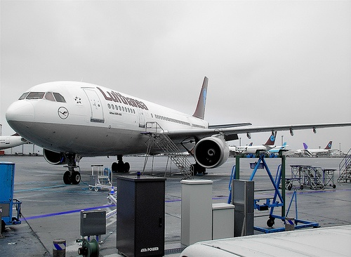
Prediction	Difference

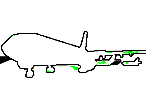
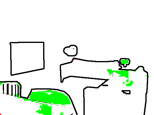
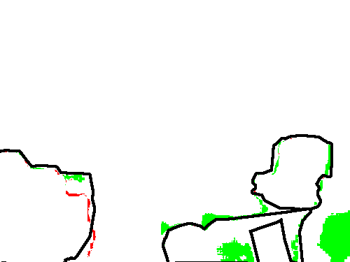
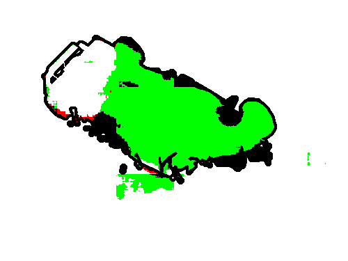
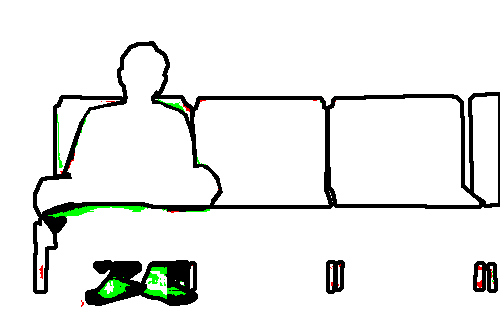
Figure 5: A comparison of predictions for the shown input images. The row labeled “Prediction Difference” shows the difference in predictions between the baseline model and the model with 11$\times$11 ($+3\times 3$) kernels in the transposed convolution. On white pixels, both models agree. Red pixels indicate that the baseline model predicts correctly but our modified model predicts incorrectly. Green pixel indicates that our modified model predicts correctly but the baseline model makes an incorrect prediction. Black pixels indicate the ground truth object segmentation boundaries for better understanding. The modification improves the segmentation result along object boundaries, which can be attributed to spectral artifact removal, but also in more extended regions, where the context plays a more crucial role.

In Table 1, we report the average PSNR and SSIM values of the reconstructed images from the GoPro test set. These results confirm that at filter size 3$\times$3, the performance of the transposed convolution variant of both the considered networks is significantly worse than the originally proposed Pixel Shuffle variant. This justifies the community’s extensive use of Pixel Shuffle for upsampling in the recent work. However, we observe on increasing context by increasing the kernel size to 7$\times$7 that the performance of the transposed convolution variants significantly improves, especially making the networks more stable when facing adversarial attacks. This boost in performance is further accentuated by increasing the kernel size to 11$\times$11 (both with parallel small kernels). These results provide evidence for Hypothesis 1.

Next, we evaluate models for semantic segmentation, where we consider highly generic architectures that allow for extensive ablations.

5.4 Semantic Segmentation

As baseline architecture for semantic segmentation, we consider a UNet-like architecture [60] with encoder backbone layers from ConvNeXt [44]. This generic architecture facilitates to provide a thorough ablation on all considered blocks in the decoder network. Our experiments are conducted on the PASCAL VOC 2012 dataset [17]. We report the mean Intersection over Union (mIoU) of the predicted and ground truth segmentation mask, the mean accuracy over all pixels (mAcc), and the mean accuracy over all classes (allAcc).

Results on Semantic Segmentation

Table 2: Semantic Segmentation performance on the PASCAL VOC2012 validation set for UNet with ConvNeXt encoder, and the baseline UNet decoder (see Figure 2) with differently sized kernels in transposed convolution for feature map upscaling.

Transposed Convolution Kernels	Test Accuracy
	mIoU	mAcc	allAcc
2$\times$2 (baseline)	78.34	86.89	95.15
7$\times$7	78.92	88.06	95.23
11$\times$11 + 3$\times$3	79.33	87.81	95.41

Table 3: Comparison of performance of models from Table 2 against adversarial attacks on UNet with ConvNeXt encoder and decoder with different sized kernels in the transposed convolution for upsampling, while keeping rest of the architecture identical. Additional results are provided in Tab. 8 and Tab. 9 in B.1.

Transposed Convolution Kernels	FGSM attack epsilon						SegPGD attack iterations
	$\frac{1}{255}$			$\frac{8}{255}$			3			20
	mIoU	mAcc	allAcc	mIoU	mAcc	allAcc	mIoU	mAcc	allAcc	mIoU	mAcc	allAcc
2$\times$2 (baseline)	53.54	70.96	86.08	47.02	65.41	82.78	23.06	46.51	45.30	5.54	18.79	23.72
7$\times$7	56.02	74.13	86.45	49.24	68.89	82.87	26.53	53.05	61.16	7.17	23.05	27.52
11$\times$11 + 3$\times$3	58.04	74.93	87.80	51.25	69.31	84.64	27.49	53.08	64.13	7.08	23.30	26.82

Table 4: FGSM adversarially trained models from Table 2 tested against SegPGD adversarial attacks on UNet with ConvNeXt encoder and decoder with different sized kernels in the transposed convolution for upsampling, while keeping rest of the architecture identical. See Tab. 8 and Tab. 9 in B.1 for more evaluations.

Transposed Convolution Kernels	Clean			SegPGD attack iterations
	Test Data			3			20
	mIoU	mAcc	allAcc	mIoU	mAcc	allAcc	mIoU	mAcc	allAcc
2$\times$2	78.57	86.68	95.23	26.59	48.99	67.71	7.6	24.06	31.37
7$\times$7	78.41	86.22	95.20	28.11	53.39	66.30	8.36	28.54	28.13
11$\times$11 + 3$\times$3	79.57	88.1	95.3	30.37	55.54	68.3	9.4	29.79	32.37

Here, we first discuss the results for different upsampling operations. The remaining architecture is kept identical, with ResNet-style building blocks in the decoder, throughout these experiments. The clean test accuracies are shown in Table 2. We see that as we increase the kernel size of the transposed convolution layers, there is a slight improvement across all three evaluation metrics. Moreover, Figure 5 visually demonstrates that, as we increase the size of the kernels in transposed convolution from 2$\times$2 in the baseline to 11$\times$11, the feature representations of the thin end and protrusions for example in the wing of the aircraft sample image are improving. The baseline model with small transposed convolution kernels could not predict these precisely. As hypothesized in H1, we observe that increasing the kernel size can reduce spectral artifacts caused when representation and images are upsampled using a transposed convolution.

In Table 3, we evaluate the performance of the segmentation models against FGSM [23] and SegPGD [27] adversarial attacks for the indicated $\epsilon$ values. As expected, with the increasing intensity of the attack, the performance of all models drops, especially for SegPGD, which is a strong multi-step attack. Yet, even at high attack intensities, the larger kernels perform better than the small ones, and we see a trend of improvement in performance as we increase the kernel size, providing more evidence for Hypothesis 1.

5.4.1 Ablation Study

In the following, we first consider the effects of additional adversarial training, then ablate on the impact of other decoder building blocks and the filter size. Variations of the model encoder are ablated in the appendix 12, the impact of using small parallel kernels in addition to large kernels is ablated and discussed in appendix B.3, and competing upsampling techniques are ablated in appendix B.4.

Adversarial Training.

In Table 4, we report results for FGSM adversarially trained models under SegPGD attack, with attacks as in Table 3. While the overall performance under attack is improved as expected, the trend of larger kernels providing better results persists. More results for FGSM attack and SegPGD attacks with different numbers of iterations are given in Tab. 8 and Tab. 9 in the Appendix. In Table 15, we additionally evaluate image restoration models under adversarial training.

Change in the decoder backbone architecture.

While all previous experiments focused on the transposed convolutions in the decoder, we here, evaluate the influence of the convolutional kernel size within the decoder which does not upsample, as explained in Section 4. For these experiments, we use a UNet architecture with a ConvNeXt backbone in the encoder and the PASCAL VOC 2012 dataset.

Table 5: Performances of UNet with ConvNeXt encoder, and decoder architectures with different sized kernels in transposed convolution and different convolution blocks in the decoder for upsampling the feature maps and decoding features respectively. Transposed Convolution with kernel size 11$\times$11+3$\times$3 performs the best with the baseline decoder building block style. For a fixed Transposed Convolution kernel size, as the size of the convolution kernel in the decoder building block is increased, the performance deteriorates.

Transposed Convolution Kernels	Decoder Building Block Style	Test Accuracy	FGSM attack epsilon		SegPGD attack iterations
		mIoU / mAcc / allAcc	$\frac{1}{255}$	$\frac{8}{255}$	3	20
			mIoU / mAcc / allAcc	mIoU / mAcc / allAcc	mIoU / mAcc / allAcc	mIoU / mAcc / allAcc
2$\times$2	ResNet Style 3$\times$3	78.34 / 86.89 / 95.15	53.54 / 70.96 / 86.08	47.02 / 65.41 / 82.78	23.06 / 46.51 / 60.04	5.54 / 18.79 / 23.72
	ConvNeXt style 7$\times$7	77.17 / 86.86 / 94.81	49.98 / 72.22 / 83.93	42.04 / 64.86 / 79.08	17.94 / 44.81 / 47.96	3.20 / 14.73 / 9.81
	ConvNeXt style 11$\times$11 + 3$\times$3	77.17 / 86.86 / 94.81	47.34 / 67.72 / 83.34	37.91 / 57.79 / 78.21	13.97 / 35.82 / 45.68	2.21 / 10.75 / 5.29
7$\times$7	ResNet Style 3$\times$3	78.92 / 88.06 / 95.23	56.02 / 74.13 / 86.45	49.24 / 68.89 / 82.87	26.53 / 53.05 / 61.16	7.17 / 23.05 / 27.52
	ConvNeXt style 7$\times$7	77.57 / 87.04 / 94.92	52.93 / 72.18 / 85.51	44.89 / 65.71 / 80.74	17.64 / 43.32 / 47.80	1.86 / 7.18 / 3.55
	ConvNeXt style 11$\times$11 + 3$\times$3	77.99 / 87.86 / 94.96	51.61 / 73.01 / 84.85	43.93 / 66.22 / 80.73	17.07 / 42.30 / 48.78	1.80 / 7.11 / 3.04
11$\times$11 + 3$\times$3	ResNet Style 3$\times$3	79.33 / 87.81 / 95.41	58.04 / 74.93 / 87.80	51.25 / 69.31 / 84.64	27.49 / 53.08 / 64.13	7.08 / 23.30 / 26.82
	ConvNeXt style 7$\times$7	78.32 / 86.98 / 95.09	53.31 / 72.45 / 86.16	44.89 / 65.18 / 82.03	16.14 / 40.65 / 50.39	1.93 / 9.35 / 3.90
	ConvNeXt style 11$\times$11 + 3$\times$3	77.42 / 86.24 / 94.94	54.48 / 72.53 / 86.25	46.67 / 66.59 / 82.29	18.76 / 44.60 / 51.49	2.31 / 8.70 / 3.50

In Table 5 we observe, for a fixed transposed convolution kernel size, as we increase the size of the convolution kernel in the decoder building blocks, the performance of the model decreases. This phenomenon extends to the performance of the architectures under adversarial attacks, showing that a mere increase in parameters in the model decoder does not have a positive effect on model performance nor on its stability. This study proves the validity of hypothesis H2. An explanation for this phenomenon could be that we only need to increase context during the actual upsampling step, increasing context in the consequent decoder building blocks has a negligible effect on the quality of representations learned. However, the increase in the number of parameters makes the architecture more susceptible to adversarial attacks.

Ablation on filter size saturation

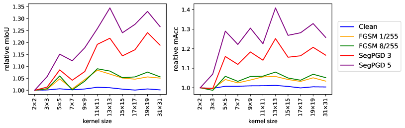
Figure 6: Comparison of performance of different sizes of transposed convolutions from standard sizes like $2\times 2$ as well as very large $31\times 31$ kernels relative to the baseline. All, besides the baseline with $2\times 2$ and $3\times 3$ have a parallel 3×3 kernel, as shown in Figure 2 (bottom left). For the decoder building block backbone, a ResNet Style $3\times 3$ style is used. These evaluations are made on PASCAL VOC2012 val dataset. We report the values in Tab. 10.

After proving H1 one could argue that networks will consistently improve with increased kernel size for the transposed convolutions. Hence, we test larger kernel sizes of 15$\times$15, 17$\times$17, 19$\times$19 and 31$\times$31 kernels. Yet, as seen in Figure 6, the effect of the kernel size appears to saturate: the performance after 13$\times$13 and the performance of 31$\times$31 kernels is not better than 11$\times$11. However, the performance of 31$\times$31 kernels is still significantly better than the baseline’s performance.

This saturation could be attributed to the quality of the encodings itself. That is, the improvement in the quality of representations learned by large upsampling kernels depends on the quality of encodings learned by the encoder. See Table 12 for more discussion.

Different Upsampling Methods

Table 6: Comparison of performances of different upsampling methods in the UNet-like architecture. All architectures here have the baseline i.e. ConvNeXt encoder and 3$\times$3 convolution kernels in the decoder block. Please refer to Table 13 in Section B.4 for more evaluations and discussion, including those with ConvNeXt style 7$\times$7+3$\times$3 Convolution kernels in the decoder blocks.

Upsampling Method	Test Accuracy			FGSM attack epsilon						SegPGD attack iterations
				$\frac{1}{255}$			$\frac{8}{255}$			5			20
	mIoU	mAcc	allAcc	mIoU	mAcc	allAcc	mIoU	mAcc	allAcc	mIoU	mAcc	allAcc	mIoU	mAcc	allAcc
Transposed Convolution 2$\times$2	78.45	86.66	95.20	53.76	70.62	86.32	47.33	64.58	83.16	14.43	35.50	45.30	5.54	18.79	23.72
Transposed Convolution 11$\times$11+3$\times$3	79.33	87.81	95.41	58.04	74.93	87.80	51.25	69.31	84.64	18.15	43.51	49.36	7.08	23.30	26.82
Pixel Shuffle	78.54	87.32	95.18	53.82	71.58	85.88	46.67	65.03	81.71	15.06	38.85	41.71	6.69	23.43	24.05
Nearest Neighbour Interpolation	78.40	88.16	95.09	52.68	73.51	84.55	46.08	67.96	80.22	15.34	44.53	36.21	7.65	27.89	20.48

Following we compare different upsampling techniques thus justifying our advocacy for using Transposed Convolution instead of other upsampling techniques like interpolation and pixel shuffle.

We report the comparison in Table 6 and observe that both Pixel shuffle and Nearest Neighbor interpolation perform better than the usually used Transposed Convolution with a 2$\times$2 kernel size. However, as we increase the kernel size for Transposed Convolution to 11$\times$11 with a 3$\times$3 small kernel in parallel, we observe that transposed convolution is strictly outperforming pixel shuffle, on both clean unperturbed images and under adversarial attacks, across all metrics used. Transposed Convolution with a large kernel is either outperforming or performing at par with Nearest Neighbor interpolation as well. Thus we demonstrate the superior clean and adversarial performance of large kernel-sized Transposed Convolution operation over other commonly used upsampling techniques. We discuss this further in Section B.4.

5.5 Disparity Estimation

Table 7: Comparison of performance of STTR-light architecture with different sized kernels in transposed convolution for upsampling the feature maps in the feature extractor (lower is better). The entire set of results is provided as Tab. 16 in Tab. 16.

Transposed Convolution Kernels	Test Accuracy		3-step PGD attack
	epe$\downarrow$	3px error$\downarrow$	epe$\downarrow$	3px error$\downarrow$
STTR-light [42] reported	0.5	1.54	-	-
3$\times$3 [42] reproduced	0.4927	1.54	4.05	18.5
7$\times$7 + 3$\times$3 (ours)	0.4788	1.50	4.02	18.3

To show that the observations extend from image restorations to other tasks, we conduct additional experiments for disparity estimation. We consider the STTR-light [42] architecture, built from STTR, which is a recent SotA ViT-based model for disparity estimation and occlusion detection. We consider the STTR-light architecture with 3$\times$3 kernels [42] in the transposed convolution layers as our baseline. To implement the proposed modification, we alter the kernel sizes in the transposed convolution layers used for pixel-wise upsampling in the “feature extractor” module of the architecture. We conduct evaluations on FlyingThings3D [50] and follow implementation details in [42].

Results for Disparity Estimation

In Table 7, we report the improvements in performance due to our architecture modification of increasing the size of the transposed convolution kernels used for upsampling, from the 3$\times$3 in the baseline model to 7$\times$7. Other kernel sizes are evaluated in Table 16 (appendix). Similar to semantic segmentation, we observe, that increasing the kernel size leads to better performance on clean images. Indicating that larger kernels in the transposed convolutions are able to better decode the learned representations from the encoder, regardless of the specific downstream task.

Similar to previous applications, the increased kernel sizes with parallel 3$\times$3 kernels further facilitate to stabilize the model when attacked, as evaluated here for 3 attack iterations using PGD with $\epsilon\approx\frac{8}{255}$ on the disparity loss.

6 Conclusion

We provide conclusive reasoning and empirical evidence for our hypotheses on the importance of context during data upsampling. While increasing the size of convolutions during upsampling increases prediction stability, increasing the size of those convolution layers without upsampling does not benefit the network in general, instead, it reduces the stability of predictions. Further, we show that our simple upsampling blocks can be directly incorporated into recent models, yielding better stability in ViT-based architectures like Restormer, NAFNet, and STTR-light as well as in classical CNNs. Our observations are consistent across several architectures and downstream tasks.

Acknowledgement.

The authors acknowledge the following: OMNI cluster of Uni Siegen computational resources, and state of Baden-Württemberg through bwHPC and the German Research Foundation (DFG) through grant INST 35/1597-1 FUGG and support by the DFG research unit 5336 - Learning to Sense.

Improving Stability during Upsampling – on the Importance of Spatial Context
Supplementary Material
In the following, we present results and figures to support our statements in the main paper and provide additional information. The following has been covered in the appendix:

• Appendix A: Detailed experimental setup for all downstream tasks.

  • Section A.1: Image Restoration experimental setup

  • Section A.2: Semantic Segmentation experimental setup

  • Section A.3: Disparity Estimation experimental setup

  • Section A.4: Detailed setup of Adversarial attacks for all downstream tasks.

  • Section A.5: Detailed setup of adversarial training for semantic segmentation and image restoration.

• Appendix B: Semantic Segmentation: Additional Experiments and Ablations. In detail:

  • Section B.1: Detailed results from Sec. 5.4 and Sec. 5.4.1.

  • Section B.1.1 : Discussion on saturation of kernel size for upsampling.

  • Section B.2: An ablation on the impact of the capacity of the encoder block for standard options such as ResNet or ConvNeXt blocks.

  • Section B.3: Ablation about including or excluding a small parallel kernel during upsampling using transposed convolution.

  • Section B.3.1 : Short study on drawbacks of using interpolation for pixel-wise upsampling.

  • Section B.4: A comparison to different kinds of upsampling Operations on Segmentation Models.

  • Section B.5: A comparison of the performance of different sized kernels in the transposed convolution operations of UNet-like models adversarially trained using FGSM attack and 3-step PGD attack on 50% of the mini-batches during training.

• Appendix C: Image Restoration : Additional Results:

  • Section C.1: Adversarial training evaluation for Restormer and NAFNet for Image deblurring task.

  • Section C.2: Qualitative results for image reconstruction models using Restormer and NAFNet and evaluated on clean data, PDG and CosPGD attack with varying numbers of attack iterations.

• Appendix D: Disparity Estimation : We provide additional results for Section 5.5: including performance against adversarial attacks.

  • Table 16 Additional discussion on the results and importance of a parallel 3$\times$3 kernel with large kernels for transposed convolution operation.

Appendix A Experimental Setup

All the experiments were done using NVIDIA V100 16GB GPUs or NVIDIA Tesla A100 40GB GPUs. For the semantic segmentation downstream task, UNet [60] was trained using 1 GPU. For the disparity estimation task, STTR-light [42] was trained using 4 NVIDIA V100 GPUs in parallel.

A.1 Image Restoration

Architectures. We consider the recently proposed state-of-the-art transformer-based Image Restoration architectures Restormer [78] and NAFNet [13]. Both architectures as proposed use Pixel Shuffle[68] to upsample feature maps. We use these as our baseline models. We replace this pixel shuffle operation with a transposed convolution operation.

Dataset. For the Image Restoration task, we focus on Image Deblurring. For this, we use the GoPro image deblurring dataset[53]. This dataset consists of 3214 real-world images with realistic blur and their corresponding ground truth (deblurred images) captured using a high-speed camera. The dataset is split into 2103 training images and 1111 test images.

Training Regime. For Restormer we follow the same training regime of progressive training as that used by Zamir et al. [78]. Similarly, for NAFNet we use the same training regime as that used by Chen et al. [13].

Evaluation Metrics. Following common practice[1, 78, 13], We report the PSNR and SSIM scores of the reconstructed images w.r.t. to the ground truth images, averaged over all images. PSNR stands for Peak Signal-to-Noise ratio, a higher PSNR indicates a better quality image or an image closer to the image to which it is being compared. SSIM stands for Structural similarity[75]. A higher SSIM score corresponds to better higher similarity between the reconstruction and the ground-truth image.

A.2 Semantic Segmentation

Here we describe the experimental setup for the segmentation task, the architectures considered, the dataset considered and the training regime.
Architectures. We considered UNet [60] with encoder layers from ConvNeXt [44]. For the decoder, the baseline comparison is done with 2$\times$2 kernels in the transposed convolution layers and the commonly used ResNet [30] BasicBlock style layers for the convolution layers in the decoder building blocks. In our experiments, we used larger sized kernels, e.g. 7$\times$7 and 11$\times$11 in the transposed convolution while keeping the rest of the architecture, including the convolution blocks in the decoder identical to Sec. 5.4. When using kernels larger than 7$\times$7 for transposed convolution we follow the work of [14, 43] and additionally include a parallel 3$\times$3 kernel to keep the local context. Usage of this parallel kernel is denoted by “+3$\times$3” Further, we analyze the behaviour of a different block of convolution layers in the decoder, as explained in Sec. 4 and replace the ResNet-style layers with ConvNeXt-style layers in Sec. 5.4.1.
Dataset. We considered the PASCAL VOC 2012 dataset [17] for the semantic segmentation task. We follow the implementation of [81, 82, 83] and augment the training examples with semantic contours from [29] as instructed by [66].
Training Regime. We follow a similar training regime as [81, 82], and train for 50 epochs, with an AdamW optimizer [47] and the learning rate was scheduled using Cosine-Annealing [46]. In the implementation of [82], the authors slide over the images using a window of size 473$\times$473, however for computation reasons and for symmetry we use a window of size 256$\times$256. We use a starting learning rate of $10^{-4}$ and a weight decay of $5\times 10^{-2}$.
Evaluation Metrics. We report the mean Intersection over Union (mIoU) of the predicted and the ground truth segmentation mask, the mean accuracy over all pixels (mAcc) and the mean accuracy over all classes (allAcc).

A.3 Disparity Estimation

Following, we describe the experimental setup for disparity estimation and occlusion detection tasks.
Architectures. We consider the STTR-light [42] architecture for our work. To analyze the influence of implementing larger kernels in transposed convolution as described in Section 4 we alter the kernel sizes in the transposed convolution layers used for pixel-wise upsampling in the “feature extractor” module of the architecture. We consider the STTR-light architecture as proposed by [42] with 3$\times$3 kernels in the transposed convolution layers as our baseline.
Dataset. Similar to [42] we train and test our models on FlyingThings3D dataset [50].
Training Regime. We follow the training regime as implemented in [42].
Evaluation Metrics. We report the end-point-error (epe) and the 3-pixel error (3px) for the disparity estimation w.r.t. the ground truth.

A.4 Adversarial Attacks

We consider the commonly used [27, 57, 77, 49] FGSM attack [23] and a new segmentation-specific SegPGD attack [27] for testing the robustness of the models against adversarial attacks. For the semantic segmentation downstream task, each crop of the input was perturbed with FGSM and SegPGD, while for the disparity estimation downstream task, each of the left and right inputs were perturbed using FGSM.
For FGSM, we test our model against epsilons $\epsilon\in\{\frac{1}{255},\frac{8}{255}\}$.

For SegPGD we follow the testing parameters as originally proposed in [27], with $\epsilon\approx\frac{8}{255}$, $\alpha$=0.01 and number of iterations $\in\{3,5,10,20,40,100\}$. We use the same scheduling for loss balancing term $\mathbf{\lambda}$ as suggested by the authors. We use SegPGD for the semantic segmentation task as it is a stronger attack specifically designed for segmentation. Thus providing more accurate insights into the models’ performance and giving a better evaluation of the architectural design choices made.

For the Image Restoration task, we follow the evaluation method of Agnihotri et al. [1], and evaluate against CosPGD[2] and PGD[41] adversarial attacks. For both attacks, we use $\epsilon\approx\frac{8}{255}$, $\alpha$=0.01 and test for number of attack iterations $\in\{5,10,20\}$.

For the Depth Estimation task, we use the PGD attack with $\epsilon\approx\frac{8}{255}$, $\alpha$=0.01 and test for number of attack iterations $\in\{5,10,20\}$.

A.5 Adversarial Training

Following, we describe the adversarial training setup employed in this work for adversarially training models for semantic segmentation and image restoration.

Semantic Segmentation.

We follow the commonly used[27] procedure and split the batch into two 50%-50% mini-batches. One mini-batch is used to generate adversarial examples using FGSM attack with $\epsilon\approx\frac{8}{255}$ and PGD attack with 3 attack iterations and with $\epsilon\approx\frac{8}{255}$ and $\alpha$=0.01 during training.

Image Restoration.

We follow the training procedure used by Agnihotri et al. [1]. We split each training batch into two equal 50%-50% mini-batches. We use one of the mini-batches to generate adversarial samples using FGSM attack with $\epsilon\approx\frac{8}{255}$.

Appendix B Additional Experiments and Ablation

Here we provide detailed results from Sec. 5 and Sec. 5.4.1 and additional results as mentioned in the main paper.

B.1 Semantic Segmentation

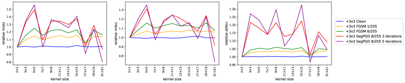
Figure 7: Comparison of performance of different sizes of transpose convolutions from standard sizes like $2\times 2$ as well as very large $31\times 31$ kernels.All have a parallel 3×3 kernel, as shown in Figure 2 (bottom left). As backbone a ConvNeXt style 11×11 +3x3 sytle is used.

Table 8 and Table 9 provide all the results of empirical performance (across the considered upsampling blocks) on clean inputs images and input images perturbed by varying intensities of FGSM and SegPGD attacks respectively.

Table 8: Complete comparison of performances against FGSM attack, of UNet with ConvNeXt encoder and decoder with architectures along with different sized kernels in transposed convolution and different convolution blocks in the decoder for upscaling the feature maps.

Transposed Convolution Kernels	Backbone Style	Test Accuracy			FGSM attack epsilon
		mIoU	mAcc	allAcc	$\epsilon$=$\frac{1}{255}$			$\epsilon$=$\frac{8}{255}$
					mIoU	mAcc	allAcc	mIoU	mAcc	allAcc
2$\times$2	ResNet Style 3$\times$3	78.34	86.89	95.15	53.54	70.96	86.08	47.02	65.41	82.78
	ConvNeXt style 7$\times$7	77.17	86.86	94.81	77.42	86.24	94.94	42.04	64.86	79.08
	ConvNeXt style 7$\times$7 + 3$\times$3	77.24	86.03	94.84	51.09	70.53	85.29	43.52	63.74	81.18
	ConvNeXt style 11$\times$11	77.68	86.42	94.97	50.73	69.78	84.88	42.33	61.80	80.36
	ConvNeXt style 11$\times$11 + 3$\times$3	77.17	86.86	94.81	47.34	67.72	83.34	37.91	57.79	78.21
3$\times$3	ResNet Style 3$\times$3	78.45	86.66	95.20	53.76	70.62	86.32	47.33	64.58	83.16
	ConvNeXt style 7$\times$7	77.70	86.89	94.99	52.30	71.56	85.73	44.80	65.38	81.99
	ConvNeXt style 7$\times$7 + 3$\times$3	77.33	87.53	94.79	50.90	72.77	83.78	44.40	67.08	79.11
	ConvNeXt style 11$\times$11	77.86	86.75	94.99	51.30	70.39	85.33	42.78	62.76	81.08
	ConvNeXt style 11$\times$11 + 3$\times$3	77.81	86.48	94.98	51.95	70.08	85.57	43.82	62.56	81.63
5$\times$5	ResNet Style 3$\times$3	79.19	87.62	95.36	55.57	73.51	86.65	48.96	67.97	83.41
	ConvNeXt style 7$\times$7	76.94	86.92	94.75	51.32	72.37	84.96	44.19	66.56	81.13
	ConvNeXt style 7$\times$7 + 3$\times$3	78.52	87.39	95.13	54.4	72.48	86.29	46.33	65.65	82.
	ConvNeXt style 11$\times$11	77.83	86.99	94.91	53.76	72.8	85.96	45.32	65.82	81.82
	ConvNeXt style 11$\times$11 + 3$\times$3	77.92	86.92	95.02	48.67	68.11	83.96	38.88	58.13	78.96
5$\times$5 + 3$\times$3	ResNet Style 3$\times$3	78.83	87.56	95.28	56.11	73.97	86.91	49.84	69.26	83.44
	ConvNeXt style 7$\times$7	78.11	86.90	95.01	53.17	71.55	86.	45.98	66.05	82.18
	ConvNeXt style 7$\times$7 + 3$\times$3	78.73	87.81	95.24	53.86	73.12	85.86	45.93	66.83	81.51
	ConvNeXt style 11$\times$11	77.83	86.57	95.07	52.12	70.29	85.79	44.05	63.11	81.63
	ConvNeXt style 11$\times$11 + 3$\times$3	77.07	86.11	94.87	54.31	72.45	86.1	47.33	66.88	82.42
7$\times$7	ResNet Style 3$\times$3	78.92	88.06	95.23	56.02	74.13	86.45	49.24	68.89	82.87
	ConvNeXt style 7$\times$7	77.57	87.04	94.92	52.93	72.18	85.51	44.89	65.71	80.74
	ConvNeXt style 7$\times$7 + 3$\times$3	77.88	87.	95.05	51.63	70.74	85.37	43.15	62.74	80.83
	ConvNeXt style 11$\times$11	77.9	87.35	94.94	53.47	72.61	85.79	45.49	67.04	81.36
	ConvNeXt style 11$\times$11 + 3$\times$3	77.99	87.86	94.96	51.61	73.01	84.85	43.93	66.22	80.73
7$\times$7 + 3$\times$3	ResNet Style 3$\times$3	78.5	87.57	95.13	53.85	72.75	85.87	47.1	67.57	82.04
	ConvNeXt style 7$\times$7	78.09	87.14	95.04	52.42	71.88	85.59	43.43	65.39	80.88
	ConvNeXt style 7$\times$7 + 3$\times$3	78.37	88.11	95.07	52.15	72.31	84.95	42.77	63.69	79.78
	ConvNeXt style 11$\times$11	77.71	87.22	94.97	52.47	73.22	85.55	44.07	65.84	81.31
	ConvNeXt style 11$\times$11 + 3$\times$3	78.14	86.94	95.05	52.08	70.63	85.98	43.82	63.65	81.95
9$\times$9	ResNet Style 3$\times$3	78.36	86.88	95.18	55.62	72.62	86.9	49.5	67.03	83.9
	ConvNeXt style 7$\times$7	77.17	86.74	94.84	52.76	72.31	85.56	44.23	64.98	81.39
	ConvNeXt style 7$\times$7 + 3$\times$3	77.93	86.97	95.04	51.01	70.59	84.87	41.93	61.63	80.18
	ConvNeXt style 11$\times$11	77.80	86.80	94.99	52.42	72.22	85.39	44.14	65.56	81.16
	ConvNeXt style 11$\times$11 + 3$\times$3	78.25	86.71	95.07	54.59	72.04	86.48	46.88	65.56	82.73
9$\times$9 + 3$\times$3	ResNet Style 3$\times$3	78.77	87.77	95.24	55.94	73.79	86.67	48.82	69.2	82.76
	ConvNeXt style 7$\times$7	77.79	86.65	94.92	52.6	70.51	85.75	43.3	62.16	80.89
	ConvNeXt style 7$\times$7 + 3$\times$3	77.96	87.24	94.98	51.21	70.01	85.24	41.75	61.16	80.64
	ConvNeXt style 11$\times$11	77.92	86.82	95.03	52.71	71.17	86.02	44.33	63.26	82.2
	ConvNeXt style 11$\times$11 + 3$\times$3	77.57	86.71	95.02	53.32	71.75	86.29	46.24	65.3	82.92
11$\times$11	ResNet Style 3$\times$3	79.11	87.06	95.36	56.18	72.11	87.27	49.51	66.15	84.12
	ConvNeXt style 7$\times$7	77.87	86.98	95.06	54.32	72.59	86.42	47.14	67.05	82.71
	ConvNeXt style 7$\times$7 + 3$\times$3	78.34	87.06	95.07	51.93	71.19	85.54	41.77	62.31	80.8
	ConvNeXt style 11$\times$11	77.42	86.68	94.94	53.11	71.43	86.03	44.55	63.45	81.75
	ConvNeXt style 11$\times$11 + 3$\times$3	77.75	86.83	95.01	52.88	71.47	85.93	43.55	62.75	81.4
11$\times$11 + 3$\times$3	ResNet Style 3$\times$3	79.33	87.81	95.41	58.04	74.93	87.8	51.25	69.31	84.64
	ConvNeXt style 7$\times$7	78.32	86.98	95.09	53.31	72.45	86.16	44.89	65.18	82.03
	ConvNeXt style 7$\times$7 + 3$\times$3	78.64	86.78	95.17	54.32	71.27	86.63	45.48	63.62	82.32
	ConvNeXt style 11$\times$11	77.15	85.93	94.87	51.19	69.72	85.45	42.02	61.09	81.1
	ConvNeXt style 11$\times$11 + 3$\times$3	77.42	86.24	94.94	54.48	72.53	86.25	46.67	66.59	82.29
13$\times$13	ResNet Style 3$\times$3	79.41	88.18	95.36	56.89	74.71	87.36	51.06	70.39	84.48
	ConvNeXt style 7$\times$7	77.99	87.11	95.06	54.96	73.32	86.69	47.39	67.2	82.73
	ConvNeXt style 7$\times$7 + 3$\times$3	78.44	87.22	95.13	54.21	72.18	86.34	47.27	65.72	82.95
	ConvNeXt style 11$\times$11	77.57	85.99	95.00	53.51	70.31	86.67	45.63	63.59	83.11
	ConvNeXt style 11$\times$11 + 3$\times$3	77.40	86.53	94.89	53.16	71.62	86.12	45.09	64.23	82.39
13$\times$13 + 3$\times$3	ResNet Style 3$\times$3	79.17	87.96	95.38	57.17	75.08	87.44	50.8	70.67	84.06
	ConvNeXt style 7$\times$7	78.05	86.73	95.02	53.41	71.62	86.12	45.07	65.04	81.76
	ConvNeXt style 7$\times$7 + 3$\times$3	77.76	86.14	95.06	54.09	72.11	86.29	45.69	65.15	82.2
	ConvNeXt style 11$\times$11	77.81	87.43	95.01	51.71	71.77	85.25	41.97	62.61	80.66
	ConvNeXt style 11$\times$11 + 3$\times$3	77.20	86.55	94.81	53.1	71.88	85.87	45.	65.01	81.91
15$\times$15	ResNet Style 3$\times$3	79.17	87.68	95.28	58.08	73.56	87.58	51.11	67.94	84.36
	ConvNeXt style 7$\times$7	78.34	87.14	95.03	53.86	72.77	86.11	45.12	65.22	81.65
	ConvNeXt style 7$\times$7 + 3$\times$3	77.39	86.40	94.95	51.2	69.42	85.27	42.65	60.88	81.24
	ConvNeXt style 11$\times$11	77.14	86.36	94.82	50.14	69.32	84.49	40.97	60.11	79.81
	ConvNeXt style 11$\times$11 + 3$\times$3	77.67	86.78	94.90	54.44	72.74	86.54	46.37	66.24	82.29
15$\times$15 + 3$\times$3	ResNet Style 3$\times$3	78.72	87.50	95.25	56.28	73.97	87.15	49.5	68.69	83.53
	ConvNeXt style 7$\times$7	77.56	87.01	94.93	53.28	72.15	85.78	45.51	64.84	81.57
	ConvNeXt style 7$\times$7 + 3$\times$3	77.09	86.27	94.76	52.25	70.01	85.41	44.01	62.49	81.16
	ConvNeXt style 11$\times$11	77.40	86.39	94.92	53.59	71.49	86.21	45.48	64.37	82.28
	ConvNeXt style 11$\times$11 + 3$\times$3	78.64	87.46	95.20	54.77	73.2	86.65	46.53	65.4	82.78
17$\times$17	ResNet Style 3$\times$3	79.22	87.77	95.37	56.5	73.3	87.27	50.1	68.23	84.11
	ConvNeXt style 7$\times$7	77.36	87.64	94.89	54.06	73.88	85.84	47.25	68.3	82.19
	ConvNeXt style 7$\times$7 + 3$\times$3	78.03	87.56	95.01	52.75	72.	85.65	44.32	64.16	81.54
	ConvNeXt style 11$\times$11	77.82	87.40	94.92	51.43	70.57	85.22	42.53	62.68	80.79
	ConvNeXt style 11$\times$11 + 3$\times$3	77.74	86.69	94.99	51.31	69.71	85.53	41.58	60.43	80.83
17$\times$17 + 3$\times$3	ResNet Style 3$\times$3	78.41	86.84	95.26	56.03	73.28	87.16	49.65	67.95	83.74
	ConvNeXt style 7$\times$7	78.14	86.99	94.98	53.44	72.34	86.01	45.02	65.35	81.85
	ConvNeXt style 7$\times$7 + 3$\times$3	78.62	87.64	95.14	55.54	73.87	86.85	47.86	67.22	83.18
	ConvNeXt style 11$\times$11	77.59	87.73	94.84	52.84	74.14	84.63	44.1	67.34	79.57
	ConvNeXt style 11$\times$11 + 3$\times$3	77.33	88.15	94.75	49.29	71.71	84.04	39.85	63.7	78.81
19$\times$19	ResNet Style 3$\times$3	78.54	87.64	95.12	56.63	74.09	87.25	50.02	68.73	83.99
	ConvNeXt style 7$\times$7	78.74	87.66	95.15	56.28	73.79	87.11	49.44	68.74	83.84
	ConvNeXt style 7$\times$7 + 3$\times$3	77.05	86.33	94.89	54.47	72.38	86.78	45.63	64.94	82.81
	ConvNeXt style 11$\times$11	77.66	86.61	95.00	51.58	71.51	84.83	42.48	63.44	79.58
	ConvNeXt style 11$\times$11 + 3$\times$3	77.61	86.59	94.93	50.34	69.39	84.54	41.82	61.29	79.75
19$\times$19 + 3$\times$3	ResNet Style 3$\times$3	78.78	87.34	95.28	56.53	74.59	86.97	50.6	69.95	83.98
	ConvNeXt style 7$\times$7	77.44	86.70	94.91	54.05	72.52	86.09	45.52	65.29	81.52
	ConvNeXt style 7$\times$7 + 3$\times$3	78.14	87.14	95.02	55.82	74.54	86.96	48.97	69.98	83.3
	ConvNeXt style 11$\times$11	78.03	86.64	95.08	53.5	71.21	86.26	45.79	64.16	82.42
	ConvNeXt style 11$\times$11 + 3$\times$3	77.42	86.61	94.91	53.83	72.54	86.17	46.29	66.94	82.22
31$\times$31	ResNet Style 3$\times$3	78.69	86.98	95.30	56.61	73.22	87.08	49.49	66.69	83.68
	ConvNeXt style 7$\times$7	77.54	87.30	94.84	52.36	72.27	85.14	43.56	65.14	8 .
	ConvNeXt style 7$\times$7 + 3$\times$3	76.96	86.38	94.77	53.59	72.14	86.05	45.22	65.22	81.84
	ConvNeXt style 11$\times$11	76.84	86.72	94.71	50.74	70.53	84.61	41.62	61.96	79.96
	ConvNeXt style 11$\times$11 + 3$\times$3	76.77	85.60	94.71	51.42	69.17	85.2	42.12	60.32	80.77
31$\times$31 + 3$\times$3	ResNet Style 3$\times$3	78.47	87.26	95.16	56.27	73.39	87.22	49.66	68.81	83.92
	ConvNeXt style 7$\times$7	77.43	86.56	94.93	53.45	72.74	86.17	45.84	66.41	82.16
	ConvNeXt style 7$\times$7 + 3$\times$3	78.43	87.07	95.17	56.72	73.65	87.6	49.56	68.15	84.22
	ConvNeXt style 11$\times$11	78.00	87.04	94.94	50.66	70.23	84.83	40.71	61.31	79.94
	ConvNeXt style 11$\times$11 + 3$\times$3	77.73	86.54	94.93	53.94	71.65	86.39	44.04	62.19	81.8

Table 9: Comparison of performances against SegPGD attack, of UNet with ConvNeXt encoder and decoder with architectures along with different sized kernels in transposed convolution and different convolution blocks in the decoder for upscaling the feature maps.

Transposed Convolution Kernels	Backbone Style	SegPGD attack iterations
		3			5			10			20			40			100
		mIoU	mAcc	allAcc	mIoU	mAcc	allAcc	mIoU	mAcc	allAcc	mIoU	mAcc	allAcc	mIoU	mAcc	allAcc	mIoU	mAcc	allAcc
2$\times$2	ResNet Style 3$\times$3	23.06	46.51	60.04	14.43	35.50	45.30	08.12	24.67	29.88	05.54	18.79	23.72	04.39	14.98	23.70	03.50	11.61	27.93
	ConvNeXt style 7$\times$7	17.94	0.4481	47.96	10.64	33.63	30.64	05.47	21.74	15.8	03.2	14.73	09.81	02.04	0.1047	0.0641	01.35	07.57	04.3
	ConvNeXt style 7$\times$7 + 3$\times$3	17.59	42.55	0.5168	09.88	30.41	0.3233	04.75	16.83	0.1431	02.65	09.46	0.0668	01.68	05.64	0.034	01.	0.0316	01.94
	ConvNeXt style 11$\times$11	16.39	0.4013	0.485	09.37	28.66	29.63	03.97	14.16	11.41	01.56	06.11	03.56	00.59	02.61	01.31	00.23	00.99	00.51
	ConvNeXt style 11$\times$11 + 3$\times$3	13.97	35.82	45.68	07.61	25.07	28.33	03.4	14.38	12.04	02.21	10.75	05.29	01.57	08.02	03.01	01.07	05.75	01.85
3$\times$3	ResNet Style 3$\times$3	23.37	46.33	60.78	15.26	38.	46.51	09.26	29.64	31.9	06.78	24.18	26.95	05.71	20.39	28.69	05.02	16.11	33.12
	ConvNeXt style 7$\times$7	18.48	43.81	54.97	09.51	29.92	34.86	03.63	15.1	13.03	01.64	08.23	04.51	01.	05.12	02.13	00.59	02.84	00.89
	ConvNeXt style 7$\times$7 + 3$\times$3	19.08	46.97	47.74	11.15	34.6	29.9	05.96	22.62	15.67	03.61	15.04	09.33	02.17	09.18	05.86	01.29	06.02	03.55
	ConvNeXt style 11$\times$11	16.2	39.11	50.93	09.52	29.32	32.61	04.93	20.31	14.82	02.86	13.94	06.46	02.05	10.94	03.58	01.4	08.23	02.21
	ConvNeXt style 11$\times$11 + 3$\times$3	18.54	41.34	55.56	10.25	30.11	36.	04.8	19.25	13.94	02.41	11.87	04.56	01.59	07.78	02.11	01.11	04.21	01.09
5$\times$5	ResNet Style 3$\times$3	24.23	51.8	57.82	16.16	42.98	43.29	10.11	32.79	30.3	07.32	25.16	27.42	06.02	19.04	31.25	05.16	14.03	37.36
	ConvNeXt style 7$\times$7	17.59	43.57	51.41	09.9	30.84	33.14	04.74	18.3	14.55	02.23	09.47	05.21	01.47	06.03	02.32	00.97	03.64	01.28
	ConvNeXt style 7$\times$7 + 3$\times$3	18.7	43.18	52.74	10.56	31.41	33.32	04.87	18.5	14.78	02.49	10.84	05.59	01.39	05.61	02.69	00.91	03.38	01.46
	ConvNeXt style 11$\times$11	18.96	44.79	53.09	09.85	29.77	32.88	03.89	14.94	12.6	01.94	08.29	04.58	01.03	04.72	01.86	00.48	02.63	00.75
	ConvNeXt style 11$\times$11 + 3$\times$3	13.38	33.61	45.	06.84	20.94	25.99	02.51	08.85	08.5	01.18	04.39	02.62	00.71	02.48	01.07	00.48	01.52	00.53
5$\times$5 + 3$\times$3	ResNet Style 3$\times$3	25.03	53.96	58.89	16.61	45.8	42.18	10.79	37.16	27.34	08.	29.62	21.71	06.16	21.69	22.25	04.83	13.87	28.97
	ConvNeXt style 7$\times$7	17.65	44.79	48.41	09.79	31.78	28.51	04.62	18.37	11.12	02.58	10.89	04.61	01.52	06.59	02.3	01.	04.04	01.33
	ConvNeXt style 7$\times$7 + 3$\times$3	18.31	42.75	49.26	09.89	28.58	30.02	03.78	12.49	11.08	01.34	04.76	03.54	00.48	02.13	01.45	00.19	00.88	00.76
	ConvNeXt style 11$\times$11	17.87	40.62	52.77	09.74	27.94	34.21	04.65	14.98	14.34	02.	05.95	04.77	01.07	02.81	01.71	00.32	00.98	00.63
	ConvNeXt style 11$\times$11 + 3$\times$3	20.84	46.95	53.91	11.86	33.96	34.86	05.65	19.8	16.66	02.83	10.73	08.2	01.59	06.21	04.68	01.11	04.2	02.62
7$\times$7	ResNet Style 3$\times$3	26.53	53.05	61.16	17.75	43.31	46.99	10.26	30.92	32.62	07.17	23.05	27.52	05.69	17.24	29.48	04.37	11.29	35.16
	ConvNeXt style 7$\times$7	17.64	43.32	47.8	09.95	30.43	28.02	04.21	15.08	10.07	01.86	07.18	03.55	00.99	03.52	01.42	00.68	01.89	00.74
	ConvNeXt style 7$\times$7 + 3$\times$3	16.64	40.11	50.56	09.75	29.72	32.23	04.95	19.4	14.47	02.87	13.23	06.4	02.06	09.55	03.45	01.59	07.24	02.04
	ConvNeXt style 11$\times$11	17.37	45.07	47.32	08.86	30.03	26.48	03.47	14.22	07.94	01.53	06.55	02.45	00.93	03.9	01.2	00.61	02.3	00.64
	ConvNeXt style 11$\times$11 + 3$\times$3	17.07	42.3	48.78	09.31	28.04	28.88	03.82	13.79	09.54	01.8	07.11	03.04	01.03	04.3	01.45	00.53	02.61	00.77
7$\times$7 + 3$\times$3	ResNet Style 3$\times$3	24.03	52.08	57.43	16.21	43.38	43.01	09.99	32.77	30.22	07.38	26.16	26.11	06.31	22.42	28.32	05.35	17.41	33.09
	ConvNeXt style 7$\times$7	16.19	43.4	48.59	09.02	32.38	29.17	04.23	19.63	10.47	02.46	12.18	03.99	01.53	06.85	01.97	00.91	03.94	01.1
	ConvNeXt style 7$\times$7 + 3$\times$3	16.04	39.67	48.16	08.94	27.45	30.33	03.81	14.69	12.79	01.91	09.17	04.63	01.2	06.16	01.95	00.84	03.96	00.95
	ConvNeXt style 11$\times$11	18.08	46.24	50.64	10.18	33.17	31.35	04.49	18.33	12.04	02.01	07.98	04.55	01.04	03.91	02.17	00.45	01.7	01.2
	ConvNeXt style 11$\times$11 + 3$\times$3	15.31	37.02	52.08	07.62	24.44	32.35	03.3	15.04	12.35	01.92	10.24	05.12	01.32	07.37	02.63	00.91	05.07	01.39
9$\times$9	ResNet Style 3$\times$3	25.26	50.75	60.85	16.88	41.02	47.16	09.44	28.03	33.87	06.23	20.76	28.91	04.71	16.45	29.14	03.69	12.63	31.93
	ConvNeXt style 7$\times$7	18.11	44.53	50.69	10.46	31.69	32.26	04.92	18.52	14.48	02.86	12.13	06.36	02.1	09.3	03.51	01.5	06.59	01.9
	ConvNeXt style 7$\times$7 + 3$\times$3	16.2	39.55	50.82	09.	28.53	33.31	04.07	17.03	15.6	02.14	10.13	07.12	01.38	05.91	03.74	00.71	02.56	01.82
	ConvNeXt style 11$\times$11	17.02	43.01	48.45	08.92	28.35	28.13	03.64	14.36	10.06	01.17	06.28	03.11	00.55	04.04	01.35	00.32	02.76	00.77
	ConvNeXt style 11$\times$11 + 3$\times$3	19.34	43.6	54.41	10.71	31.22	33.98	04.6	15.76	12.75	01.98	07.78	04.04	00.95	03.95	01.69	00.51	01.96	00.78
9$\times$9 + 3$\times$3	ResNet Style 3$\times$3	24.87	55.04	57.35	17.	46.34	42.08	10.88	36.04	28.55	07.91	28.17	22.86	06.02	21.13	22.87	04.63	14.45	27.39
	ConvNeXt style 7$\times$7	16.56	36.5	53.58	08.74	23.95	35.67	04.01	13.92	16.64	02.13	08.87	06.34	01.38	06.37	02.27	01.01	04.8	01.11
	ConvNeXt style 7$\times$7 + 3$\times$3	16.03	36.92	51.5	08.8	25.53	33.15	03.64	13.95	12.25	01.61	06.02	04.08	00.83	02.72	01.83	00.37	01.13	00.87
	ConvNeXt style 11$\times$11	16.42	39.19	51.71	08.32	26.64	31.11	03.66	15.7	11.61	01.94	10.11	04.4	01.19	06.75	02.23	00.83	04.83	01.36
	ConvNeXt style 11$\times$11 + 3$\times$3	18.72	41.83	55.48	10.38	29.7	36.72	04.74	18.16	17.44	02.49	11.2	07.18	01.69	08.21	03.56	01.24	06.07	01.93
11$\times$11	ResNet Style 3$\times$3	26.02	48.81	63.76	16.8	39.62	49.72	09.62	29.4	34.22	06.85	24.07	27.66	05.63	20.38	26.45	04.56	15.64	28.86
	ConvNeXt style 7$\times$7	19.04	45.39	52.63	10.17	32.3	32.46	04.58	20.16	13.36	02.44	13.63	05.33	01.74	10.13	03.04	01.21	07.07	01.7
	ConvNeXt style 7$\times$7 + 3$\times$3	16.08	39.09	53.1	08.86	28.27	35.06	03.94	16.77	15.75	02.25	11.87	06.31	01.32	07.98	02.72	00.82	05.14	01.28
	ConvNeXt style 11$\times$11	18.09	40.72	53.7	09.93	29.6	34.68	04.55	18.22	14.17	02.21	10.51	05.2	01.38	06.35	02.34	00.96	03.84	01.28
	ConvNeXt style 11$\times$11 + 3$\times$3	15.29	37.2	50.71	07.6	25.19	30.65	03.17	15.06	09.58	01.78	10.21	03.07	01.3	07.74	01.39	01.	05.6	00.88
11$\times$11 + 3$\times$3	ResNet Style 3$\times$3	27.49	53.08	64.13	18.15	43.51	49.36	10.29	31.12	33.17	07.08	23.3	26.82	05.14	16.14	27.32	03.77	09.6	31.61
	ConvNeXt style 7$\times$7	16.14	40.65	50.39	08.08	27.2	31.4	03.34	15.36	12.29	01.93	09.35	03.9	01.36	05.77	01.76	00.92	03.51	00.83
	ConvNeXt style 7$\times$7 + 3$\times$3	17.7	39.71	54.64	09.71	26.92	35.8	04.32	13.93	15.8	02.37	08.49	06.7	01.59	05.85	03.43	01.09	03.87	01.83
	ConvNeXt style 11$\times$11	14.62	34.73	49.37	07.26	22.21	29.37	02.76	12.24	10.69	01.23	07.06	04.16	00.71	04.71	01.96	00.63	03.65	00.96
	ConvNeXt style 11$\times$11 + 3$\times$3	18.76	44.6	51.49	10.07	31.15	30.26	04.4	17.02	10.56	02.31	08.7	03.5	01.34	04.85	01.66	00.73	02.56	00.81
13$\times$13	ResNet Style 3$\times$3	28.51	57.18	63.94	19.71	48.99	50.08	11.99	37.69	33.26	08.31	28.29	26.23	06.17	21.38	25.65	04.83	15.34	29.52
	ConvNeXt style 7$\times$7	20.9	46.62	55.13	12.32	34.21	35.91	06.14	21.39	16.39	03.15	13.44	07.51	02.16	10.21	04.3	01.41	06.61	02.54
	ConvNeXt style 7$\times$7 + 3$\times$3	20.13	42.92	57.7	11.38	29.96	39.57	04.85	15.81	19.37	02.54	09.48	09.47	01.65	06.45	05.61	00.86	03.83	03.
	ConvNeXt style 11$\times$11	18.65	39.48	56.4	10.02	27.46	38.02	04.69	17.27	19.03	02.47	11.35	08.76	01.39	07.95	04.12	00.9	06.02	02.11
	ConvNeXt style 11$\times$11 + 3$\times$3	18.95	42.88	55.82	10.68	31.21	35.69	04.92	18.29	12.63	02.35	09.29	03.78	01.26	05.02	01.6	00.79	02.56	00.72
13$\times$13 + 3$\times$3	ResNet Style 3$\times$3	28.08	58.22	63.4	19.4	50.01	48.89	12.04	39.2	32.11	08.77	31.09	24.9	06.46	22.51	23.98	04.34	13.59	28.41
	ConvNeXt style 7$\times$7	18.42	43.52	51.26	10.23	30.56	30.5	04.37	16.41	11.29	02.08	09.09	04.39	01.35	06.65	02.49	00.86	04.28	01.37
	ConvNeXt style 7$\times$7 + 3$\times$3	16.7	41.09	50.56	08.54	26.94	30.39	03.31	13.44	11.22	01.53	06.72	04.13	01.02	04.01	02.01	00.56	02.07	01.03
	ConvNeXt style 11$\times$11	14.1	36.4	47.79	07.01	23.32	27.54	02.87	12.05	10.26	01.51	06.85	04.56	01.13	05.21	03.2	01.13	05.21	03.2
	ConvNeXt style 11$\times$11 + 3$\times$3	18.14	43.14	52.31	09.55	28.16	32.41	03.54	12.57	11.22	01.52	06.19	03.35	00.97	03.66	01.52	00.65	02.11	00.84
15$\times$15	ResNet Style 3$\times$3	29.41	51.54	66.7	19.96	41.26	55.14	11.51	29.26	41.04	07.17	20.8	31.7	05.13	15.79	28.53	03.9	11.59	29.37
	ConvNeXt style 7$\times$7	18.62	44.42	51.51	10.55	32.47	32.54	04.69	18.66	12.4	02.64	11.81	04.44	01.67	07.93	02.02	01.29	05.26	01.21
	ConvNeXt style 7$\times$7 + 3$\times$3	17.63	37.55	55.52	09.13	23.28	37.06	03.46	09.05	15.8	01.41	03.5	06.96	00.77	01.62	04.02	00.51	01.04	02.48
	ConvNeXt style 11$\times$11	15.24	36.62	49.45	08.05	24.89	31.93	03.68	14.62	13.68	02.03	07.68	05.66	01.26	04.48	03.25	00.61	02.51	01.87
	ConvNeXt style 11$\times$11 + 3$\times$3	19.01	44.78	52.74	10.35	31.98	32.35	04.38	19.15	12.42	02.31	12.1	04.84	01.53	07.72	02.24	01.06	04.86	01.17
15$\times$15 + 3$\times$3	ResNet Style 3$\times$3	26.38	53.79	61.59	17.9	45.03	47.36	10.79	33.9	31.75	07.14	25.02	25.01	05.43	18.97	25.39	04.18	13.25	30.47
	ConvNeXt style 7$\times$7	19.81	42.18	53.73	11.14	28.25	37.03	04.72	13.45	17.41	01.92	05.27	07.64	01.06	03.07	04.37	00.7	01.97	02.61
	ConvNeXt style 7$\times$7 + 3$\times$3	17.53	39.4	54.39	09.51	26.67	35.52	03.73	12.39	13.27	00.93	04.2	03.22	00.44	02.14	01.01	00.16	00.94	00.36
	ConvNeXt style 11$\times$11	16.69	39.29	52.18	08.78	27.55	32.8	03.72	17.08	12.37	02.06	11.89	03.94	01.38	08.59	02.	00.99	06.41	01.24
	ConvNeXt style 11$\times$11 + 3$\times$3	19.15	41.08	55.96	10.71	29.12	37.58	05.28	19.35	18.54	02.88	13.69	08.43	02.	11.2	04.47	01.41	09.	02.39
17$\times$17	ResNet Style 3$\times$3	27.74	53.24	64.48	18.51	43.47	51.02	10.72	32.21	36.08	07.43	25.5	28.78	05.85	20.69	28.85	04.93	16.94	32.03
	ConvNeXt style 7$\times$7	19.82	46.01	54.48	11.09	32.71	36.79	05.35	19.1	17.49	02.67	10.25	07.1	01.87	07.1	02.98	01.25	04.64	01.33
	ConvNeXt style 7$\times$7 + 3$\times$3	16.96	38.94	54.19	09.23	26.92	36.22	04.47	16.8	16.9	02.45	11.16	07.09	01.61	08.12	03.53	01.03	05.47	01.95
	ConvNeXt style 11$\times$11	13.72	34.03	48.09	06.57	20.94	26.93	02.32	09.22	07.84	01.08	04.61	02.28	00.63	02.55	01.	00.35	01.33	00.47
	ConvNeXt style 11$\times$11 + 3$\times$3	14.47	33.55	52.16	07.33	20.91	32.91	02.82	09.75	13.11	01.28	04.95	04.96	00.79	03.01	02.52	00.47	01.55	01.32
17$\times$17 + 3$\times$3	ResNet Style 3$\times$3	26.97	54.13	62.04	18.41	45.5	47.66	11.05	34.55	32.01	07.43	25.65	24.78	05.07	17.38	24.12	03.51	10.48	27.4
	ConvNeXt style 7$\times$7	17.96	41.81	54.93	09.08	27.73	35.7	03.85	15.38	15.51	01.95	09.2	05.76	01.17	05.74	02.35	00.86	03.99	01.25
	ConvNeXt style 7$\times$7 + 3$\times$3	19.86	42.55	56.89	10.29	28.26	37.83	04.43	15.77	16.52	01.93	08.45	06.36	01.	05.27	02.61	00.68	03.7	01.31
	ConvNeXt style 11$\times$11	16.84	44.91	45.35	09.41	31.25	26.04	03.8	14.79	09.08	01.4	05.56	02.83	00.47	02.05	01.03	00.17	01.1	00.54
	ConvNeXt style 11$\times$11 + 3$\times$3	14.06	38.28	46.37	06.95	24.78	27.4	02.92	14.65	10.36	01.55	09.22	03.9	00.96	06.21	02.04	00.68	04.61	01.29
19$\times$19	ResNet Style 3$\times$3	27.64	52.62	64.53	18.46	42.79	51.19	10.49	30.27	36.37	06.92	22.02	28.21	05.17	17.07	26.09	03.99	12.16	27.92
	ConvNeXt style 7$\times$7	20.28	46.96	56.75	10.06	30.29	36.2	03.5	13.07	14.56	01.51	06.13	05.64	00.72	03.24	02.4	00.64	02.2	01.4
	ConvNeXt style 7$\times$7 + 3$\times$3	18.14	39.86	56.98	09.34	26.13	37.16	03.5	13.58	14.24	01.52	07.79	04.4	00.83	05.76	01.83	00.54	03.82	00.93
	ConvNeXt style 11$\times$11	15.85	40.55	46.13	08.33	28.21	25.47	03.27	15.94	07.52	01.8	10.44	02.95	01.3	07.65	01.81	00.97	05.34	01.22
	ConvNeXt style 11$\times$11 + 3$\times$3	16.17	37.68	50.29	08.47	25.22	31.86	03.84	14.74	13.88	01.93	08.84	06.27	01.2	05.41	03.28	00.79	03.68	02.02
19$\times$19 + 3$\times$3	ResNet Style 3$\times$3	28.62	56.15	63.93	19.19	47.17	48.9	10.96	34.41	31.54	07.15	25.67	23.6	05.25	19.32	21.84	04.24	15.12	24.17
	ConvNeXt style 7$\times$7	17.45	40.44	51.24	09.13	27.29	31.41	03.56	13.76	10.77	01.61	06.83	03.35	00.94	04.	01.37	00.56	02.22	00.54
	ConvNeXt style 7$\times$7 + 3$\times$3	20.9	48.61	54.54	11.59	35.05	33.3	04.6	18.94	11.57	02.05	10.9	03.51	01.42	07.83	01.63	00.9	05.28	00.88
	ConvNeXt style 11$\times$11	19.01	41.41	55.17	10.56	28.9	37.54	05.23	19.35	17.13	02.92	12.99	07.27	02.05	09.7	03.82	01.42	07.14	02.18
	ConvNeXt style 11$\times$11 + 3$\times$3	17.98	44.39	52.86	09.44	30.77	32.15	03.36	14.64	09.76	01.14	05.22	02.06	00.48	02.49	00.6	00.17	01.16	00.26
31$\times$31	ResNet Style 3$\times$3	26.44	50.1	63.1	17.8	39.96	50.81	10.44	29.22	36.6	06.67	21.09	28.13	04.91	16.07	23.92	03.65	10.93	23.02
	ConvNeXt style 7$\times$7	17.75	41.69	51.94	09.26	27.63	32.32	03.52	12.48	11.73	01.37	04.95	04.18	00.62	02.57	01.93	00.37	01.68	01.02
	ConvNeXt style 7$\times$7 + 3$\times$3	16.53	40.82	50.9	08.	25.9	30.59	02.79	11.15	10.24	01.24	05.19	03.11	00.56	02.42	01.12	00.34	01.4	00.53
	ConvNeXt style 11$\times$11	13.08	31.95	45.87	05.85	17.71	25.83	02.06	07.35	08.65	00.88	03.15	02.74	00.39	01.55	01.05	00.26	01.15	00.55
	ConvNeXt style 11$\times$11 + 3$\times$3	15.42	35.92	51.53	07.44	21.84	31.72	02.43	09.33	10.18	00.85	03.85	02.59	00.41	01.79	01.04	00.22	00.99	00.56
31$\times$31 + 3$\times$3	ResNet Style 3$\times$3	27.41	54.28	64.15	18.27	44.66	49.97	11.02	33.64	34.65	07.24	25.06	26.54	05.39	18.81	22.82	04.3	14.03	22.46
	ConvNeXt style 7$\times$7	18.76	40.98	55.63	10.33	28.32	38.72	04.95	18.11	19.82	02.74	12.53	08.41	01.69	08.6	03.73	01.03	05.94	01.75
	ConvNeXt style 7$\times$7 + 3$\times$3	20.55	44.15	58.99	10.65	30.05	40.0	04.69	17.49	18.07	02.65	11.74	07.33	01.6	08.05	03.37	01.09	05.88	01.79
	ConvNeXt style 11$\times$11	14.47	36.3	49.11	07.12	22.87	29.65	02.57	11.14	10.67	01.24	06.52	03.69	00.9	05.06	01.68	00.63	03.65	00.96
	ConvNeXt style 11$\times$11 + 3$\times$3	13.59	32.71	49.91	06.09	18.39	29.59	01.96	06.7	08.76	00.79	02.53	02.11	00.4	01.47	00.89	00.12	00.65	00.45

B.1.1 Limit of large kernels for Upsampling

Table 10: Comparison of performance of very large: 31$\times$31 kernels in transposed convolution to large (7$\times$7 to 17$\times$17) kernels. All have a parallel 3$\times$3 kernel, as shown in Figure 2 (bottom left). Here we observe the saturation of performance for very large kernels for upsampling. This comparison is for the same encoder (ConvNeXt) and same ResNet-like building blocks in the decoder (our baseline). The complete table is provided in Section B.1.

Transposed Convolution Kernels	Test Accuracy			FGSM attack epsilon						SegPGD attack iterations
	mIoU	mAcc	allAcc	$\frac{1}{255}$			$\frac{8}{255}$			20
				mIoU	mAcc	allAcc	mIoU	mAcc	allAcc	mIoU	mAcc	allAcc
7$\times$7	78.50	87.57	95.13	53.85	72.75	85.87	47.10	67.57	82.04	7.38	26.16	26.11
11$\times$11	79.33	87.81	95.41	58.04	74.93	87.80	51.25	69.31	84.64	7.08	23.30	26.82
15$\times$15	78.72	87.50	95.25	56.28	73.97	87.15	49.50	68.69	83.53	7.14	25.02	25.01
17$\times$17	78.41	86.84	95.26	56.03	73.28	87.16	49.65	67.95	83.74	7.43	25.65	24.78
19$\times$19	78.78	87.34	95.28	56.53	74.59	86.97	50.60	69.95	83.98	7.15	25.67	23.60
31$\times$31	78.47	87.26	95.16	56.27	73.39	87.22	49.66	68.81	83.92	7.24	25.06	26.54

As discussed in Sec. 5.4.1, the performance of large kernels begins to saturate at a point. We report results from Figure 6 in tabular form in Table 10. In Table 10, we find that 13$\times$13 appears to be the saturation point for this setting and 31$\times$31 kernels are beyond this saturation point. While 31$\times$31 performs worse or on-par with 17$\times$17, it still performs significantly better than the baseline of 2$\times$2. We find that these results further strengthen our Hypothesis 2. For ease of understanding, we visualize the trends from Table 10 in Figure 7.

B.2 Choice of encoder

Table 11: Comparison of performances of different encoders in the UNet-like architecture. All architectures here have the baseline 2$\times$2 transposed convolution kernel for upsampling followed by 3$\times$3 convolution kernels in the decoder blocks. For more results please refer to Table 12.

Encoder	Test Accuracy			FGSM attack epsilon						SegPGD attack iterations
				$\frac{1}{255}$			$\frac{8}{255}$			20
	mIoU	mAcc	allAcc	mIoU	mAcc	allAcc	mIoU	mAcc	allAcc	mIoU	mAcc	allAcc
ResNet50	67.69	79.04	92.80	36.78	58.41	78.16	32.60	52.63	74.56	4.98	19.28	21.07
ConvNeXt tiny	78.45	86.66	95.20	53.76	70.62	86.32	47.33	64.58	83.16	5.54	18.79	23.72
SLaK tiny	78.82	87.01	95.17	55.22	71.72	86.97	48.69	66.45	83.57	8.45	25.42	32.37

Table 12: Comparison of performances of different encoders in the UNet-like architecture. All architectures here have the baseline 2$\times$2 transposed convolution kernel followed by 3$\times$3 convolution kernels in the decoder block.

Encoder	Test Accuracy			FGSM attack epsilon						SegPGD attack iterations
				$\frac{1}{255}$			$\frac{8}{255}$			3			5			10			20			40			100
	mIoU	mAcc	allAcc	mIoU	mAcc	allAcc	mIoU	mAcc	allAcc	mIoU	mAcc	allAcc	mIoU	mAcc	allAcc	mIoU	mAcc	allAcc	mIoU	mAcc	allAcc	mIoU	mAcc	allAcc	mIoU	mAcc	allAcc
ResNet50	67.69	79.04	92.80	36.78	58.41	78.16	32.60	52.63	74.56	16.18	37.46	50.04	11.32	30.59	38.98	7.21	23.76	27.58	4.98	19.28	21.07	3.95	16.49	18.35	3.09	13.87	15.87
ConvNeXt tiny	78.45	86.66	95.20	53.76	70.62	86.32	47.33	64.58	83.16	23.06	46.51	60.04	14.43	35.50	45.30	8.12	24.67	29.88	5.54	18.79	23.72	4.39	14.98	23.70	3.50	11.61	27.93
SLaK tiny	78.82	87.01	95.17	55.22	71.72	86.97	48.69	66.45	83.57	26.71	50.92	64.04	19.28	43.51	52.88	12.24	33.65	39.78	8.45	25.42	32.37	6.22	19.58	29.06	-	-	-

Following we aim to understand the importance of the encoder and its influence on the quality of representations later decoded during the upsampling. Consequently, we justify our choice of using ConvNeXt tiny encoder for the majority of our studies.

In Table 11 we compare different encoders: ResNet50, ConvNeXt tiny, and SLaK [43] while fixing the decoder to the baseline implementation. All encoders are pre-trained on the ImageNet-1k training dataset.

We observe that using ConvNeXt tiny and SLaK as the encoder backbone gives us significantly better performance than using ResNet50 as the encoder. This observation holds true for both clean and adversarially perturbed samples. We additionally observe that SLaK gives us marginally better performance than ConvNeXt. As shown by Liu et al. [43], SLaK is a significantly better encoder than ConvNeXt tiny as it provides significantly more context than ConvNeXt by using kernel sizes up to 51$\times$51 in the convolution layers during encoding. This proves that better encoding can be harnessed during decoding which can lead to better upsampling.

However, in this work, we used the ConvNeXt tiny encoder since the SLaK encoder takes significantly longer to train for only a marginal gain in performance. We report the performance results in Table 12. We observe that given our computation budget and the wall-clock time limit of 24 hours, we are unable to even compute the performance of the model with the SLaK encoder at 100 attack iterations.

B.3 Ablation over small parallel kernel

Following we ablate over use of a small (3$\times$3) kernel in parallel to a large ($\geq$7$\times$7) kernel for transposed convolution. This concept is inspired by [14, 43] who use a small kernel in parallel with the large kernels to preserve local context when downsampling. Similar behaviour is observed while upsampling. Table 8 compares the usage of this small parallel kernel. We observe, that while not using the small kernel results in marginal better performance on clean images (for a fixed backbone style), it lacks context and thus performs poorly (when compared to using a small parallel kernel) against adversarial attacks.

This is further highlighted in Table 9 when the performance is compared against strong adversarial attacks. Moreover, we observe that from medium-sized kernels i.e. , the upsampling seems to lose local context, and adding a kernel in parallel helps the model in getting this additional context. This effect can also be observed in the adversarial performances of the respective models.

B.3.1 Drawbacks of interpolation

As discussed in Section 3, architecture designs that use interpolation for pixel-wise upsampling suffer with over-smoothening of feature maps. This can be seen in the final predictions, as shown in Fig. 8(b) compared to the ground truth segmentation mask in Fig. 8(a) and prediction from a model with 11$\times$11 + 3$\times$3 transposed convolution kernel in Fig. 8(c).

In their work, Gu et al. [27] showed that PSPNet has considerably lower performance against adversarial attacks, similar to the analysis made in Section 5.4.1. This is explained by H2.

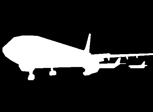
(a) Ground truth segmentation mask of the third image in the test set.

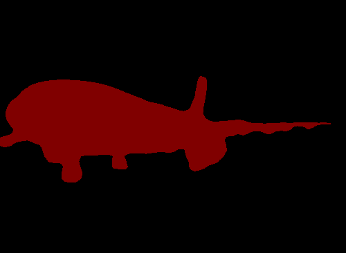
(b) Prediction from PSPNet with ResNet 50 backbone as implemented by the authors.

(c) Prediction when using 11$\times$11 + 3$\times$3 kernel sizes in transposed convolution layers and 3$\times$3 convolution kernels in the decoder building blocks of UNet.

Figure 8: A comparison of difference in the sharpness of final predictions due to different upsampling techniuqes. Fig. 8(a) is the ground truth segmenation mask with sharp and thin edges in the rear fin and wing with protrusions in the wing of the aircraft. We observe that PSPNet with a ResNet50 backbone as implemented by [82] is not able to accurately predict the thin edges and the protrusions, and is simply smoothening them out. This is due to the interpolation operation used in upsampling. However in comparison, as shown in Fig. 8(c), when a transposed convolution operation is used for pixel-wise upsampling, the thin edges are more sharp and protrusions are more accurately predicted.

B.4 Different Upsampling Methods

Following, we continue the discussion from Section 5.4.1 and compare different upsampling techniques thus justifying our advocacy for using Transposed Convolution instead of other upsampling techniques like interpolation and pixel shuffle.

We report the comparison in Table 6 and observe that both Pixel shuffle and Nearest Neighbor interpolation perform better than the usually used Transposed Convolution with a 2$\times$2 kernel size. However, as we increase the kernel size for Transposed Convolution to 11$\times$11 with a 3$\times$3 small kernel in parallel, we observe that transposed convolution is strictly outperforming pixel shuffle, on both clean unperturbed images and under adversarial attacks, across all metrics used. Transposed Convolution with a large kernel is either outperforming or performing at par with Nearest Neighbor interpolation as well. Thus we demonstrate the superior clean and adversarial performance of large kernel-sized Transposed Convolution operation over other commonly used upsampling techniques.

Table 13: Comparison of performances of different upsampling methods in the UNet-like architecture. All architectures here have the baseline i.e. ConvNeXt encoder and a ResNet style 3$\times$3 or ConvNext style 7 $\times$7+3$\times$3 convolution kernels in the decoder block.

Upsampling Method	Convolution Kernel in Decoder blocks	Test Accuracy			FGSM attack epsilon						SegPGD attack iterations
					$\frac{1}{255}$			$\frac{8}{255}$			3			5			10			20			40			100
		mIoU	mAcc	allAcc	mIoU	mAcc	allAcc	mIoU	mAcc	allAcc	mIoU	mAcc	allAcc	mIoU	mAcc	allAcc	mIoU	mAcc	allAcc	mIoU	mAcc	allAcc	mIoU	mAcc	allAcc	mIoU	mAcc	allAcc
Transposed Convolution 2$\times$2	ResNet Style 3$\times$3	78.45	86.66	95.20	53.76	70.62	86.32	47.33	64.58	83.16	23.06	46.51	60.04	14.43	35.50	45.30	8.12	24.67	29.88	5.54	18.79	23.72	4.39	14.98	23.70	3.50	11.61	27.93
	ConvNeXt Style 7$\times$7+3$\times$3	77.24	86.03	94.84	51.09	70.53	85.29	43.52	63.74	81.18	17.59	42.55	51.68	9.88	30.41	32.33	4.75	16.83	14.31	2.65	9.46	6.68	1.68	5.64	3.4	1.0	3.16	1.94
Transposed Convolution 11$\times$11+3$\times$3	ResNet Style 3$\times$3	79.33	87.81	95.41	58.04	74.93	87.8	51.25	69.31	84.64	27.49	53.08	64.13	18.15	43.51	49.36	10.29	31.12	33.17	7.08	23.3	26.82	5.14	16.14	27.32	3.77	9.6	31.61
	ConvNeXt Style 7$\times$7+3$\times$3	78.64	86.78	95.17	54.32	71.27	86.63	45.48	63.62	82.32	17.7	39.71	54.64	9.71	26.92	35.8	4.32	13.93	15.8	2.37	8.49	6.7	1.59	5.85	3.43	1.09	3.87	1.83
Pixel Shuffle	ResNet Style 3$\times$3	78.54	87.32	95.18	53.82	71.58	85.88	46.67	65.03	81.71	23.08	48.18	56.54	15.06	38.85	41.71	9.17	29.43	28.17	6.69	23.43	24.05	5.69	19.61	25.71	4.80	15.53	32.10
	ConvNeXt Style 7$\times$7+3$\times$3	77.10	85.90	94.88	51.78	69.68	85.44	43.80	62.24	81.06	17.52	40.16	50.31	9.43	27.37	30.37	3.53	12.25	10.93	1.41	5.42	3.74	0.78	3.04	1.55	0.52	1.96	0.93
Nearest Neighbour Interpolation	ResNet Style 3$\times$3	78.40	88.16	95.09	52.68	73.51	84.55	46.08	67.96	80.22	22.82	53.16	51.75	15.34	44.53	36.21	10.02	34.83	23.84	7.65	27.89	20.48	6.43	23.23	21.48	5.40	17.34	28.05
	ConvNeXt Style 7$\times$7+3$\times$3	77.86	86.92	94.97	50.71	71.21	84.45	41.97	64.92	78.89	15.77	44.36	42.09	8.56	30.25	23.74	2.96	12.56	7.19	1.27	5.70	2.10	0.52	2.08	0.75	0.17	0.85	0.35

There might be speculation if other downsampling techniques are able to utilize larger convolution kernels in the decoder building blocks better than transposed convolution. Thus, we additionally experiment using a ConvNeXt-like 7$\times$7+3$\times$3 kernel in the Convolution operations in the decoder building blocks that follow the upsampling operation. We report these results in Table 13 and observe that similar to transposed convolution, other upsampling methods also do not benefit from an increase in the kernel size in the decoder building blocks.

B.5 Adversarial Training

Table 14: Adversarially trained models from Table 2 tested against adversarial attacks on UNet with ConvNeXt encoder and decoder with different sized kernels in the transposed convolution for upscaling, while keeping rest of the architecture identical.

Transposed Convolution Kernels	Clean Test Accuracy			FGSM attack epsilon						SegPGD attack iterations
				$\frac{1}{255}$			$\frac{8}{255}$			3			20
	mIoU	mAcc	allAcc	mIoU	mAcc	allAcc	mIoU	mAcc	allAcc	mIoU	mAcc	allAcc	mIoU	mAcc	allAcc
FGSM training
2$\times$2 (baseline)	78.57	86.68	95.23	54.28	70.80	86.91	52.45	68.38	86.26	26.59	48.99	67.71	7.6	24.06	31.37
7$\times$7	78.41	86.22	95.20	56.87	72.92	87.70	51.31	68.4	85.17	28.11	53.39	66.30	8.36	28.54	28.13
11$\times$11 + 3$\times$3	79.57	88.1	95.3	57.90	74.64	87.61	52.15	70.23	84.96	30.37	55.54	68.3	9.4	29.79	32.37
PGD training with 3 attack iterations
2$\times$2 (baseline)	75.33	84.66	94.39	53.87	72.17	86.58	58.57	73.93	89.01	29.38	57.82	66.67	9.39	33.15	28.11
7$\times$7	75.79	84.89	94.38	54.82	72.31	86.80	61.29	74.33	89.96	31.12	58.36	68.58	10.24	33.99	31.14
11$\times$11 + 3$\times$3	75.90	86.60	94.30	56.27	75.66	86.68	63.02	76.17	90.42	33.50	58.34	71.50	10.77	32.23	37.36

Following, we present the results from adversarial training for semantic segmentation. In Table 14, we report the performance of different transposed convolution kernel-sized adversarially trained UNet on clean input and adversarially perturbed inputs. We observe, the improvement in performance when increasing the transposed convolution kernel size during normal training also extends to adversarial training.

Appendix C Additional Results on Image Restoration

Following we provide additional results for the Image deblurring tasks, like the performance of models after adversarial training and some visual results of the deblurring for a better understanding of the impact of increased spatial context against different adversarial attack methods and strengths.

C.1 Adversarial Training

Table 15: Comparison of performances of adversarially trained SotA Image Restoration Networks. The considered architectures use Pixel Shuffle for Upsampling, we propose replacing the Pixel Shuffle with Transposed Convolution operations using the large filter. Testing for image deblurring on GoPro dataset.

Network	Upsampling Method	Test Accuracy		PGD attack iterations
				5		10		20
		PSNR	SSIM	PSNR	SSIM	PSNR	SSIM	PSNR	SSIM
NAFNet + ADV	Pixel Shuffle	29.91	0.9291	15.76	0.5228	13.91	0.4445	12.73	0.3859
	Transposed Conv 3$\times$3	31.26	0.9448	15.89	0.5390	13.43	0.4627	11.62	0.4098
	Transposed Conv 7$\times$7 + 3 $\times$3 (Ours)	31.21	0.9446	16.46	0.5061	14.55	0.4211	13.31	0.3688
	Transposed Conv 11$\times$11 + 3$\times$3 (Ours)	30.70	0.9390	13.68	0.4857	11.91	0.4085	10.92	0.3604

In Table 15 we provide additional results for adversarially training image restoration network NAFNet using FGSM attack on 50% of the training minibatch of the GoPro dataset each iteration. The state-of-the-art Image Restoration models are significantly larger w.r.t. the number of parameters, compared to the models considered for semantic segmentation. Thus, they are significantly more difficult to train adversarially. They require more training iterations. Due to the limited computing budget, we have only trained them for the same iterations as clean (non-adversarial) training iterations. We already observe the advantages of using a larger kernel for transposed convolution over pixel-shuffle in these experiments.

C.2 Visual Results

Figure 9 shows reconstruction under PGD attack for Restormer [78] and NAFNet [13].

MODEL			NO ATTACK	5 iterations	10 iterations	20 iterations
Restormer	with Pixel Shuffle
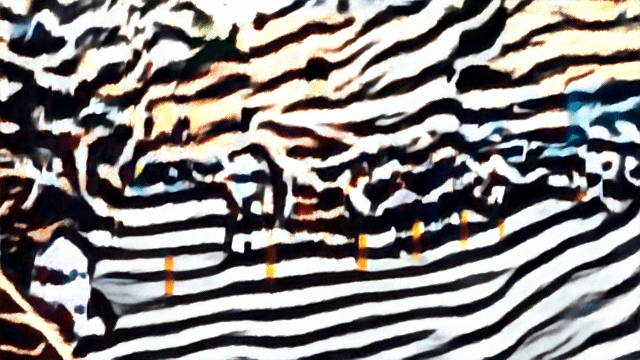
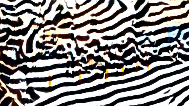
Restormer	with Transposed Conv	3$\times$3
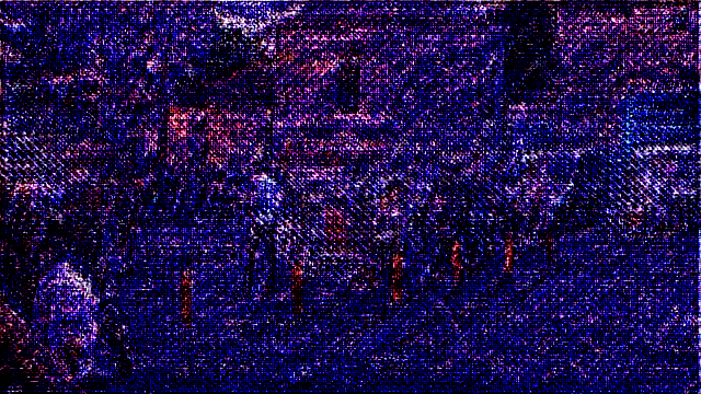
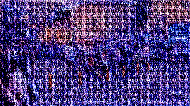
Restormer	with Transposed Conv	7$\times$7 + 3$\times$3
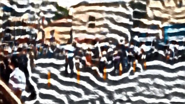
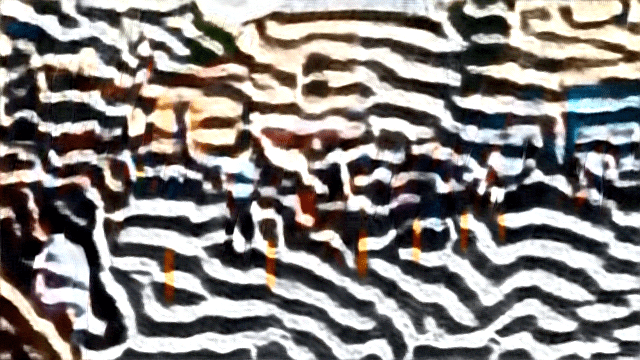
Restormer	with Transposed Conv	11$\times$11 + 3$\times$3
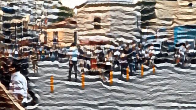
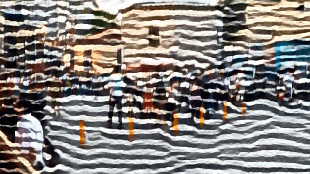
NAFNet	with Pixel Shuffle
NAFNet	with Transposed Conv	3$\times$3
NAFNet	with Transposed Conv	7$\times$7 + 3$\times$3
NAFNet	with Transposed Conv	11$\times$11 + 3$\times$3

Figure 9: Comparing images reconstructed by all models after PGD attack on variants of Upsampling.

Figure 10 shows reconstruction under CosPGD attack for Restormer [78] and NAFNet [13].

MODEL			NO ATTACK	5 iterations	10 iterations	20 iterations
Restormer	with Pixel Shuffle
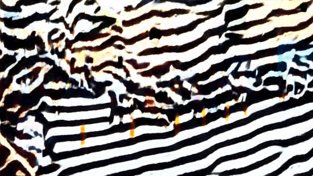
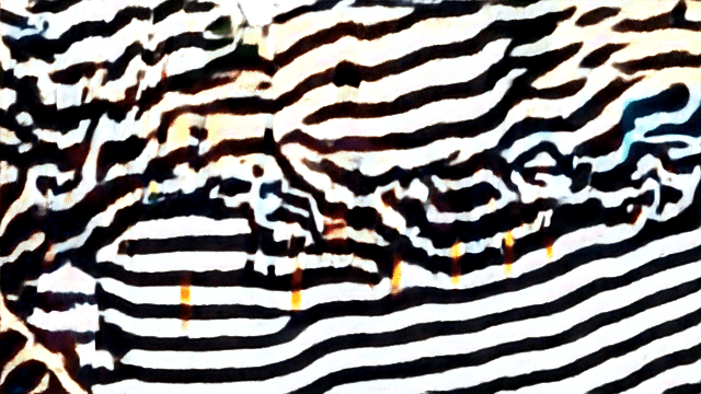
Restormer	with Transposed Conv	3$\times$3
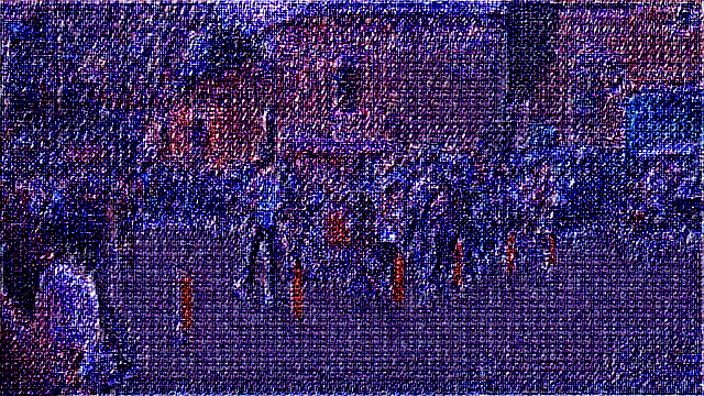
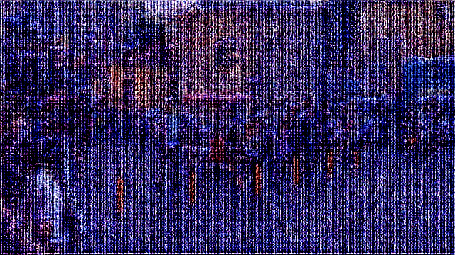
Restormer	with Transposed Conv	7$\times$7 + 3$\times$3
Restormer	with Transposed Conv	11$\times$11 + 3$\times$3
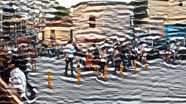
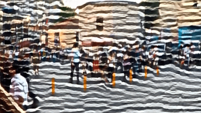
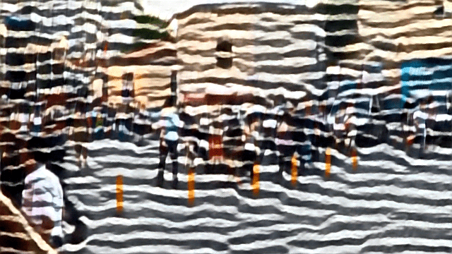
NAFNet	with Pixel Shuffle
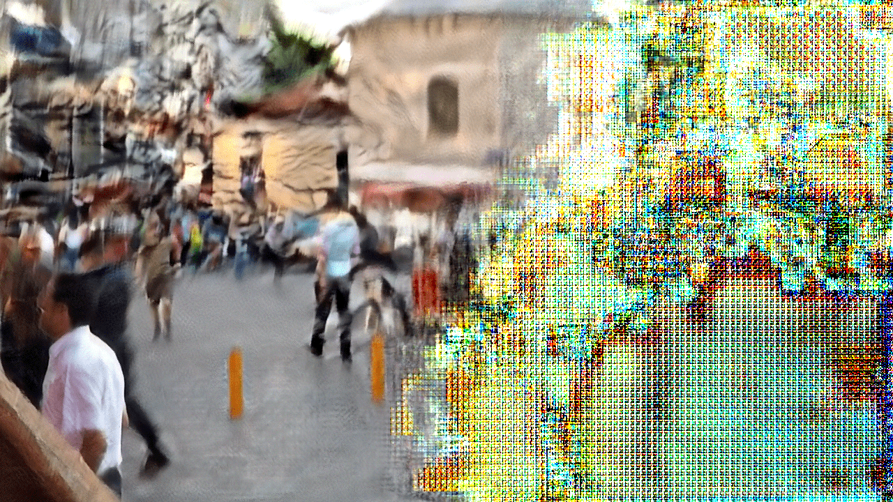
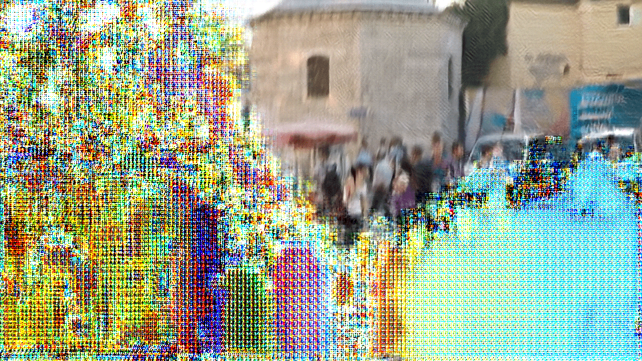
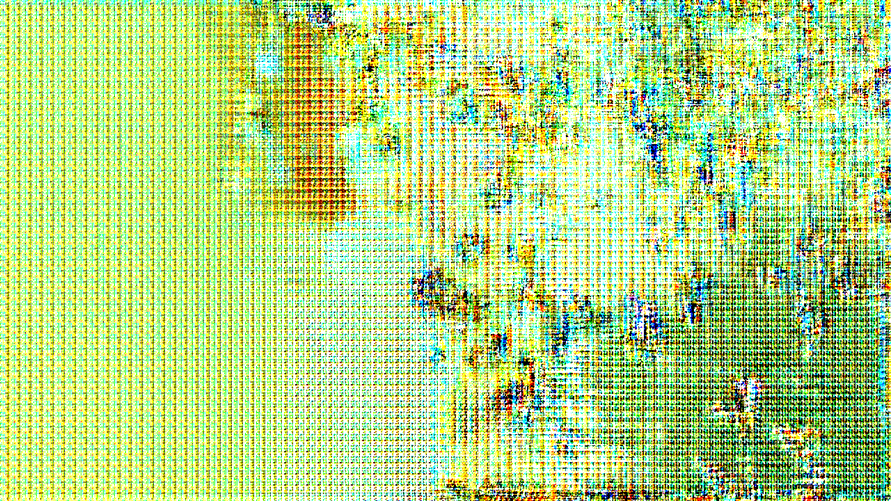
NAFNet	with Transposed Conv	3$\times$3
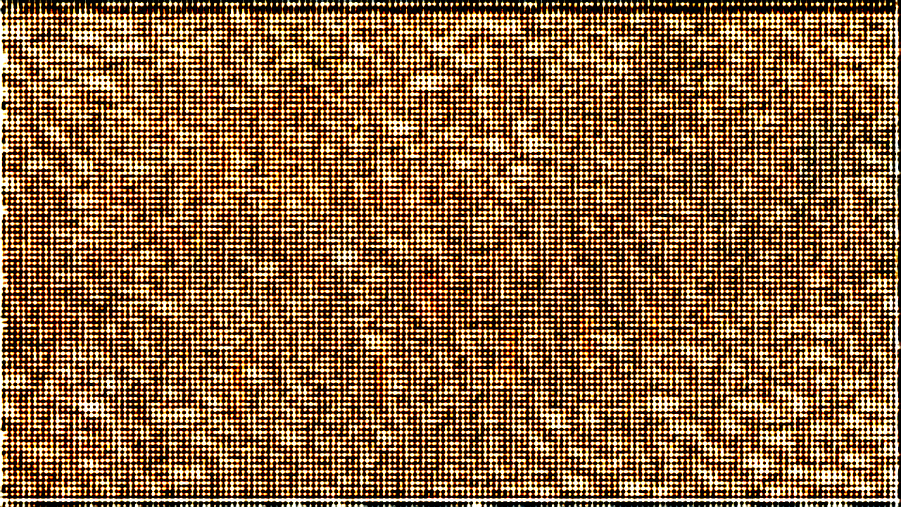
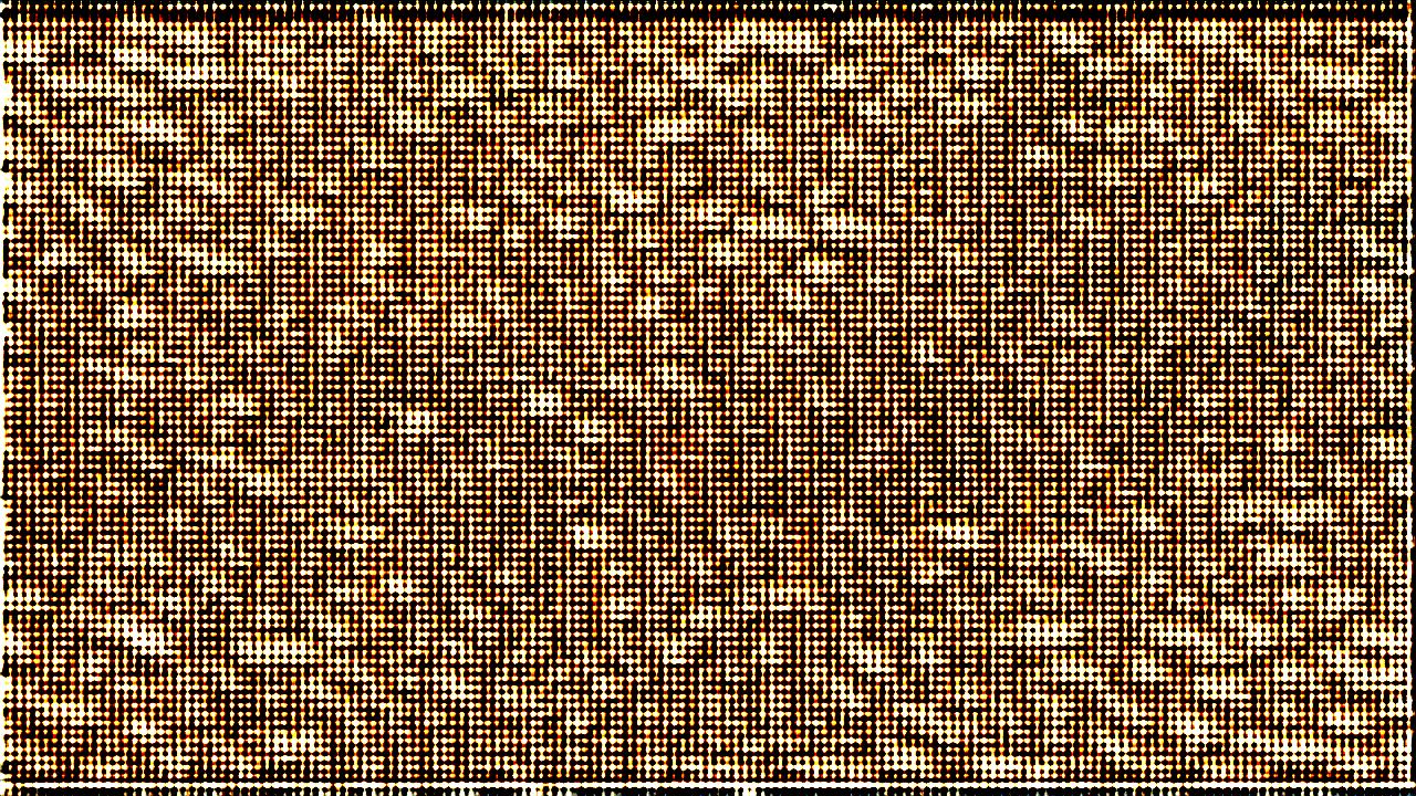
NAFNet	with Transposed Conv	7$\times$7 + 3$\times$3
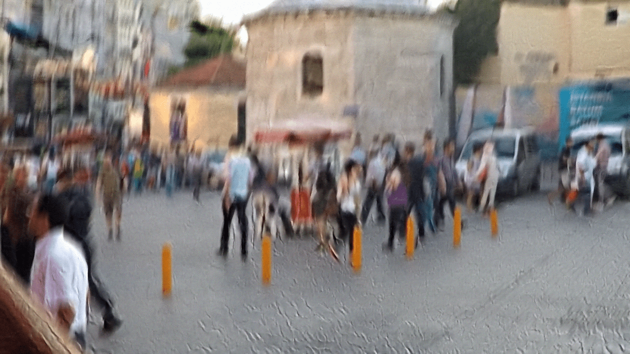
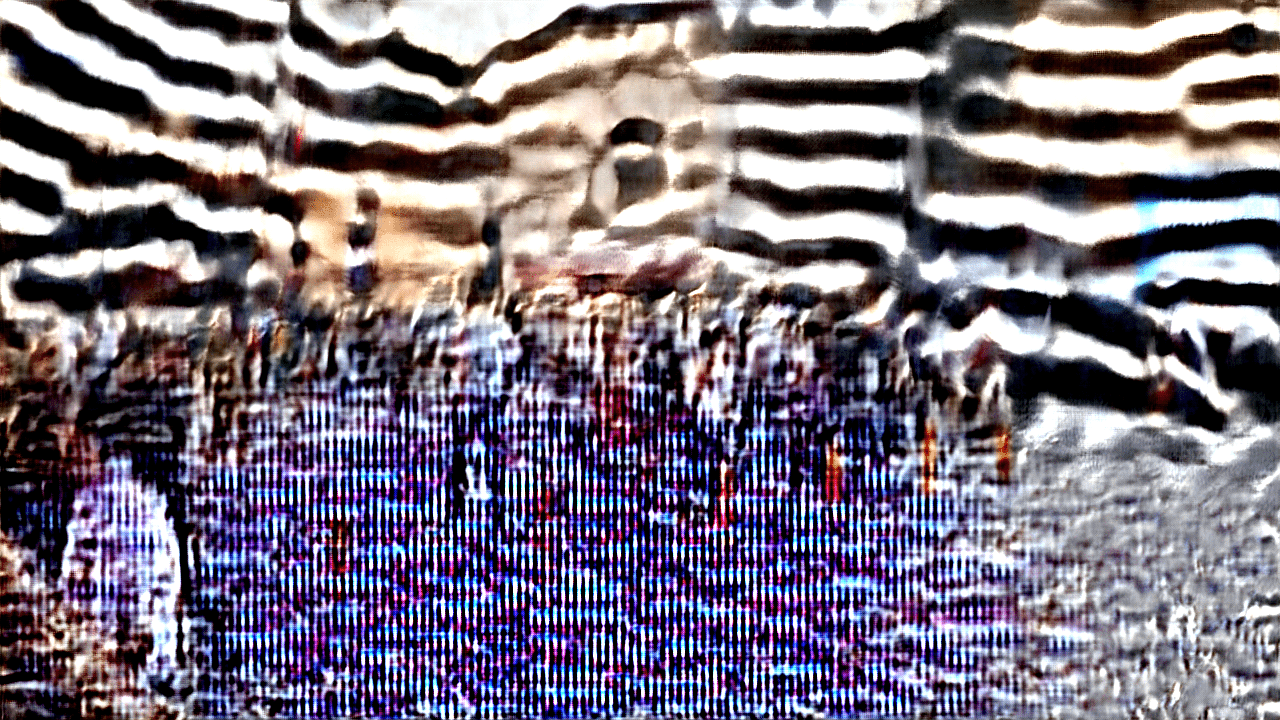
NAFNet	with Transposed Conv	11$\times$11 + 3$\times$3

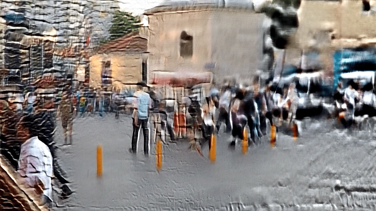
Figure 10: Comparing images reconstructed by the considered variants of the SotA models after CosPGD attack [2]. We observe that the originally proposed Restormer and NAFNet architectures that use Pixel Shuffle for upsampling perform considerably well under no adversarial attack but even a small perturbation of $\epsilon$=$\frac{8}{255}$ causes ringing and other spectral artifacts to occur in the deblurred images to the extent that the images are unrecognizable. However, on replacing the Pixel Shuffle operation in these architectures with a Transposed Convolution operation with a large kernel (11$\times$11+3$\times$3), we observe a significant reduction in the spectral artifacts in the images restored under adversarial attack while the image restored under no attack are very comparable to those restored by the original architectures.

.

Appendix D Additional Results Disparity Estimation

Following we report additional results for Disparity Estimation using STTR-light. In Table 16 we report the performance of STTR-light architecture on clean test images and under PGD attack. Whereas in Figure 11, we present a visual comparison of depth estimation predictions by a vanilla STTR-light as proposed by Li et al. [42] and our proposed modification of increasing the kernel size of the transposed convolution operation in the “feature extractor” module of the architecture from 3$\times$3 to 7$\times$7+3$\times$3 and 11$\times$11+3$\times$3.

D.1 Disparity Estimation Discussion

Table 16: Comparison of performance of STTR-light architecture with different sized kernels in transposed convolution for upscaling the feature maps in the feature extractor.

Transposed Convolution Kernels	Test Accuracy		PGD Attack
			3 Iterations		5 Iterations		10 Iterations
	epe$\downarrow$	3px error$\downarrow$	epe$\downarrow$	3px error$\downarrow$	epe$\downarrow$	3px error$\downarrow$	epe$\downarrow$	3px error$\downarrow$
STTR-light [42] reported	0.5	1.54
3$\times$3 [42] reproduced	0.4927	1.54	4.05	18.46	4.07	18.59	4.08	18.6
7$\times$7	0.487	1.52	4.26	19.09	4.289	19.21	4.294	19.23
7$\times$7 + 3$\times$3	0.4788	1.50	4.02	18.3	4.0474	18.43	4.05	18.45
9$\times$9	0.4983	1.50	4.36	18.02	4.386	18.14	4.39	18.16
11$\times$11 +3$\times$3	0.5124	1.57	4.004	18.29	4.028	18.42	4.032	18.44

In Figure 11 as shown by the region in the red circle, both vanilla architecture and the architecture with our proposed change perform well compared to the ground truth on clean images. However, under 10 iteration PGD adversarial attack, we observe small protrusion’s depth(shown by the red arrow) is incorrectly estimated by the vanilla architecture. The architecture with 7$\times$7+3$\times$3 and 11$\times$11+3$\times$3 transposed convolution kernels preserves the prediction of the depth.

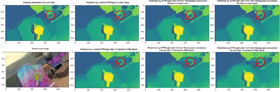
Figure 11: Visual comparison of depth estimation predictions by a vanilla STTR-light as proposed by Li et al. [42] and our proposed modification of increasing the kernel size of the transposed convolution operation in the “feature extractor” module of the architecture from 3$\times$3 to 7$\times$7+3$\times$3. As shown by the region in the red circle, both vanilla architecture and the architecture with our proposed change perform well compared to the ground truth on clean images. However, under 10 iteration PGD adversarial attack, we observe small protrusion’s depth(shown by the red arrow) is incorrectly estimated by the vanilla architecture, however the architecture with 7$\times$7+3$\times$3 transposed convolution kernel preserves the prediction of the depth.

Additionally from Table 16, we observe the significance of the parallel 3$\times$3 small kernel with the large 7$\times$7 and 11$\times$11 kernels. The performance of the large kernels without the small parallel kernel is significantly work.

References

- Agnihotri et al. [2023a] Shashank Agnihotri, Kanchana Vaishnavi Gandikota, Julia Grabinski, Paramanand Chandramouli, and Margret Keuper. On the unreasonable vulnerability of transformers for image restoration-and an easy fix. In Proceedings of the IEEE/CVF International Conference on Computer Vision, pages 3707–3717, 2023a.
- Agnihotri et al. [2023b] Shashank Agnihotri, Steffen Jung, and Margret Keuper. Cospgd: a unified white-box adversarial attack for pixel-wise prediction tasks, 2023b.
- Aitken et al. [2017] Andrew Aitken, Christian Ledig, Lucas Theis, Jose Caballero, Zehan Wang, and Wenzhe Shi. Checkerboard artifact free sub-pixel convolution: A note on sub-pixel convolution, resize convolution and convolution resize. arXiv preprint arXiv:1707.02937, 2017.
- Ba et al. [2016] Jimmy Lei Ba, Jamie Ryan Kiros, and Geoffrey E. Hinton. Layer normalization, 2016.
- Badki et al. [2020] Abhishek Badki, Alejandro Troccoli, Kihwan Kim, Jan Kautz, Pradeep Sen, and Orazio Gallo. Bi3D: Stereo depth estimation via binary classifications. In The IEEE Conference on Computer Vision and Pattern Recognition (CVPR), 2020.
- Badrinarayanan et al. [2015] Vijay Badrinarayanan, Alex Kendall, and Roberto Cipolla. Segnet: A deep convolutional encoder-decoder architecture for image segmentation, 2015.
- Baranchuk et al. [2021] Dmitry Baranchuk, Ivan Rubachev, Andrey Voynov, Valentin Khrulkov, and Artem Babenko. Label-efficient semantic segmentation with diffusion models, 2021.
- Carion et al. [2020] Nicolas Carion, Francisco Massa, Gabriel Synnaeve, Nicolas Usunier, Alexander Kirillov, and Sergey Zagoruyko. End-to-end object detection with transformers, 2020.
- Carlini and Wagner [2017] Nicholas Carlini and David Wagner. Towards evaluating the robustness of neural networks. In 2017 ieee symposium on security and privacy (sp), pages 39–57. IEEE, 2017.
- Caron et al. [2020] Mathilde Caron, Ishan Misra, Julien Mairal, Priya Goyal, Piotr Bojanowski, and Armand Joulin. Unsupervised learning of visual features by contrasting cluster assignments, 2020.
- Chandrasegaran et al. [2021] Keshigeyan Chandrasegaran, Ngoc-Trung Tran, and Ngai-Man Cheung. A closer look at fourier spectrum discrepancies for cnn-generated images detection. In Proceedings of the IEEE/CVF Conference on Computer Vision and Pattern Recognition (CVPR), pages 7200–7209, 2021.
- Chang and Chen [2018] Jia-Ren Chang and Yong-Sheng Chen. Pyramid stereo matching network, 2018.
- Chen et al. [2022] Liangyu Chen, Xiaojie Chu, Xiangyu Zhang, and Jian Sun. Simple baselines for image restoration. In European Conference on Computer Vision, pages 17–33. Springer, 2022.
- Ding et al. [2022] Xiaohan Ding, Xiangyu Zhang, Yizhuang Zhou, Jungong Han, Guiguang Ding, and Jian Sun. Scaling up your kernels to 31x31: Revisiting large kernel design in cnns, 2022.
- Dumoulin and Visin [2016] Vincent Dumoulin and Francesco Visin. A guide to convolution arithmetic for deep learning. arXiv preprint arXiv:1603.07285, 2016.
- Durall et al. [2020] Ricard Durall, Margret Keuper, and Janis Keuper. Watch your up-convolution: Cnn based generative deep neural networks are failing to reproduce spectral distributions. In Proceedings of the IEEE/CVF conference on computer vision and pattern recognition, pages 7890–7899, 2020.
- Everingham et al. [2012] M. Everingham, L. Van Gool, C. K. I. Williams, J. Winn, and A. Zisserman. The PASCAL Visual Object Classes Challenge 2012 (VOC2012) Results. http://www.pascal-network.org/challenges/VOC/voc2012/workshop/index.html, 2012.
- Fischer et al. [2015] Philipp Fischer, Alexey Dosovitskiy, Eddy Ilg, Philip Häusser, Caner Hazırbaş, Vladimir Golkov, Patrick van der Smagt, Daniel Cremers, and Thomas Brox. Flownet: Learning optical flow with convolutional networks, 2015.
- Forsyth and Ponce [2003] D. Forsyth and J. Ponce. Computer Vision: A Modern Approach. Prentice Hall, 2003.
- Gal et al. [2021] Rinon Gal, Dana Cohen Hochberg, Amit Bermano, and Daniel Cohen-Or. Swagan: A style-based wavelet-driven generative model. ACM Transactions on Graphics (TOG), 40(4):1–11, 2021.
- Geirhos et al. [2018] Robert Geirhos, Patricia Rubisch, Claudio Michaelis, Matthias Bethge, Felix A Wichmann, and Wieland Brendel. Imagenet-trained cnns are biased towards texture; increasing shape bias improves accuracy and robustness. In International Conference on Learning Representations, 2018.
- Goodfellow et al. [2020] Ian Goodfellow, Jean Pouget-Abadie, Mehdi Mirza, Bing Xu, David Warde-Farley, Sherjil Ozair, Aaron Courville, and Yoshua Bengio. Generative adversarial networks. Communications of the ACM, 63(11):139–144, 2020.
- Goodfellow et al. [2014] Ian J. Goodfellow, Jonathon Shlens, and Christian Szegedy. Explaining and harnessing adversarial examples, 2014.
- Grabinski et al. [2022a] Julia Grabinski, Steffen Jung, Janis Keuper, and Margret Keuper. Frequencylowcut pooling–plug & play against catastrophic overfitting. arXiv preprint arXiv:2204.00491, 2022a.
- Grabinski et al. [2022b] Julia Grabinski, Janis Keuper, and Margret Keuper. Aliasing coincides with cnns vulnerability towards adversarial attacks. In The AAAI-22 Workshop on Adversarial Machine Learning and Beyond, pages 1–5, 2022b.
- Grabinski et al. [2022c] Julia Grabinski, Janis Keuper, and Margret Keuper. Aliasing and adversarial robust generalization of cnns. Machine Learning, pages 1–27, 2022c.
- Gu et al. [2022] Jindong Gu, Hengshuang Zhao, Volker Tresp, and Philip Torr. Segpgd: An effective and efficient adversarial attack for evaluating and boosting segmentation robustness, 2022.
- Guo et al. [2022] Meng-Hao Guo, Cheng-Ze Lu, Qibin Hou, Zhengning Liu, Ming-Ming Cheng, and Shi-Min Hu. Segnext: Rethinking convolutional attention design for semantic segmentation, 2022.
- Hariharan et al. [2011] Bharath Hariharan, Pablo Arbelaez, Lubomir Bourdev, Subhransu Maji, and Jitendra Malik. Semantic contours from inverse detectors. In International Conference on Computer Vision (ICCV), 2011.
- He et al. [2015] Kaiming He, Xiangyu Zhang, Shaoqing Ren, and Jian Sun. Deep residual learning for image recognition, 2015.
- He et al. [2021] Yang He, Ning Yu, Margret Keuper, and Mario Fritz. Beyond the spectrum: Detecting deepfakes via re-synthesis. In Proceedings of the Thirtieth International Joint Conference on Artificial Intelligence, IJCAI-21, pages 2534–2541. International Joint Conferences on Artificial Intelligence Organization, 2021. Main Track.
- Hendrycks and Gimpel [2016] Dan Hendrycks and Kevin Gimpel. Gaussian error linear units (gelus), 2016.
- Hoffmann et al. [2021] J Hoffmann, S Agnihotri, Tonmoy Saikia, and Thomas Brox. Towards improving robustness of compressed cnns. In ICML Workshop on Uncertainty and Robustness in Deep Learning (UDL), 2021.
- Hossain et al. [2021] Md Tahmid Hossain, Shyh Wei Teng, Ferdous Sohel, and Guojun Lu. Anti-aliasing deep image classifiers using novel depth adaptive blurring and activation function, 2021.
- Howard et al. [2017] Andrew G. Howard, Menglong Zhu, Bo Chen, Dmitry Kalenichenko, Weijun Wang, Tobias Weyand, Marco Andreetto, and Hartwig Adam. Mobilenets: Efficient convolutional neural networks for mobile vision applications, 2017.
- Huang et al. [2016] Gao Huang, Zhuang Liu, Laurens van der Maaten, and Kilian Q. Weinberger. Densely connected convolutional networks, 2016.
- Ilg et al. [2016] Eddy Ilg, Nikolaus Mayer, Tonmoy Saikia, Margret Keuper, Alexey Dosovitskiy, and Thomas Brox. Flownet 2.0: Evolution of optical flow estimation with deep networks, 2016.
- Jung and Keuper [2021] Steffen Jung and Margret Keuper. Spectral distribution aware image generation. In Proceedings of the AAAI conference on artificial intelligence, pages 1734–1742, 2021.
- Karras et al. [2021] Tero Karras, Miika Aittala, Samuli Laine, Erik Härkönen, Janne Hellsten, Jaakko Lehtinen, and Timo Aila. Alias-free generative adversarial networks. Advances in Neural Information Processing Systems, 34:852–863, 2021.
- Khayatkhoei and Elgammal [2022] Mahyar Khayatkhoei and Ahmed Elgammal. Spatial frequency bias in convolutional generative adversarial networks. In Proceedings of the AAAI Conference on Artificial Intelligence, pages 7152–7159, 2022.
- Kurakin et al. [2017] Alexey Kurakin, Ian Goodfellow, and Samy Bengio. Adversarial machine learning at scale, 2017.
- Li et al. [2020] Zhaoshuo Li, Xingtong Liu, Nathan Drenkow, Andy Ding, Francis X. Creighton, Russell H. Taylor, and Mathias Unberath. Revisiting stereo depth estimation from a sequence-to-sequence perspective with transformers, 2020.
- Liu et al. [2022a] Shiwei Liu, Tianlong Chen, Xiaohan Chen, Xuxi Chen, Qiao Xiao, Boqian Wu, Mykola Pechenizkiy, Decebal Mocanu, and Zhangyang Wang. More convnets in the 2020s: Scaling up kernels beyond 51x51 using sparsity, 2022a.
- Liu et al. [2022b] Zhuang Liu, Hanzi Mao, Chao-Yuan Wu, Christoph Feichtenhofer, Trevor Darrell, and Saining Xie. A convnet for the 2020s, 2022b.
- Long et al. [2015] Jonathan Long, Evan Shelhamer, and Trevor Darrell. Fully convolutional networks for semantic segmentation. In Proceedings of the IEEE conference on computer vision and pattern recognition, pages 3431–3440, 2015.
- Loshchilov and Hutter [2016] Ilya Loshchilov and Frank Hutter. Sgdr: Stochastic gradient descent with warm restarts, 2016.
- Loshchilov and Hutter [2017] Ilya Loshchilov and Frank Hutter. Decoupled weight decay regularization, 2017.
- Maiya et al. [2021] Shishira R Maiya, Max Ehrlich, Vatsal Agarwal, Ser-Nam Lim, Tom Goldstein, and Abhinav Shrivastava. A frequency perspective of adversarial robustness, 2021.
- Mathew et al. [2020] Alwyn Mathew, Aditya Patra, and Jimson Mathew. Monocular depth estimators: Vulnerabilities and attacks. ArXiv, abs/2005.14302, 2020.
- Mayer et al. [2016] N. Mayer, E. Ilg, P. Häusser, P. Fischer, D. Cremers, A. Dosovitskiy, and T. Brox. A large dataset to train convolutional networks for disparity, optical flow, and scene flow estimation. In IEEE International Conference on Computer Vision and Pattern Recognition (CVPR), 2016. arXiv:1512.02134.
- Moosavi-Dezfooli et al. [2016] Seyed-Mohsen Moosavi-Dezfooli, Alhussein Fawzi, and Pascal Frossard. Deepfool: a simple and accurate method to fool deep neural networks. In Proceedings of the IEEE conference on computer vision and pattern recognition, pages 2574–2582, 2016.
- Mosleh et al. [2014] Ali Mosleh, J. M. Pierre Langlois, and Paul Green. Image deconvolution ringing artifact detection and removal via psf frequency analysis. In Computer Vision – ECCV 2014, pages 247–262, Cham, 2014. Springer International Publishing.
- Nah et al. [2017] Seungjun Nah, Tae Hyun Kim, and Kyoung Mu Lee. Deep multi-scale convolutional neural network for dynamic scene deblurring. In CVPR, 2017.
- Noh et al. [2015] Hyeonwoo Noh, Seunghoon Hong, and Bohyung Han. Learning deconvolution network for semantic segmentation. In Proceedings of the IEEE international conference on computer vision, pages 1520–1528, 2015.
- Odena et al. [2016] Augustus Odena, Vincent Dumoulin, and Chris Olah. Deconvolution and checkerboard artifacts. Distill, 2016.
- Peng et al. [2017] Chao Peng, Xiangyu Zhang, Gang Yu, Guiming Luo, and Jian Sun. Large kernel matters – improve semantic segmentation by global convolutional network. In Proceedings of the IEEE Conference on Computer Vision and Pattern Recognition (CVPR), 2017.
- Pervin et al. [2021] Mst. Tasnim Pervin, Linmi Tao, Aminul Huq, Zuoxiang He, and Li Huo. Adversarial attack driven data augmentation for accurate and robust medical image segmentation, 2021.
- Radford et al. [2015] Alec Radford, Luke Metz, and Soumith Chintala. Unsupervised representation learning with deep convolutional generative adversarial networks. arXiv preprint arXiv:1511.06434, 2015.
- Radosavovic et al. [2020] Ilija Radosavovic, Raj Prateek Kosaraju, Ross Girshick, Kaiming He, and Piotr Dollar. Designing network design spaces. In Proceedings of the IEEE/CVF Conference on Computer Vision and Pattern Recognition (CVPR), 2020.
- Ronneberger et al. [2015] Olaf Ronneberger, Philipp Fischer, and Thomas Brox. U-net: Convolutional networks for biomedical image segmentation, 2015.
- Scheurer et al. [2023] Erik Scheurer, Jenny Schmalfuss, Alexander Lis, and Andrés Bruhn. Detection defenses: An empty promise against adversarial patch attacks on optical flow. arXiv preprint arXiv:2310.17403, 2023.
- Schmalfuss et al. [2022a] Jenny Schmalfuss, Lukas Mehl, and Andrés Bruhn. Attacking motion estimation with adversarial snow. arXiv preprint arXiv:2210.11242, 2022a.
- Schmalfuss et al. [2022b] Jenny Schmalfuss, Philipp Scholze, and Andrés Bruhn. A perturbation-constrained adversarial attack for evaluating the robustness of optical flow, 2022b.
- Schmalfuss et al. [2023] Jenny Schmalfuss, Lukas Mehl, and Andrés Bruhn. Distracting downpour: Adversarial weather attacks for motion estimation, 2023.
- Schott et al. [2018] Lukas Schott, Jonas Rauber, Matthias Bethge, and Wieland Brendel. Towards the first adversarially robust neural network model on mnist. In International Conference on Learning Representations, 2018.
- segcv [2021] segcv. segcv/pspnet. https://github.com/segcv/PSPNet/blob/master/Train.md, 2021.
- Shannon [1949] C.E. Shannon. Communication in the presence of noise. Proceedings of the IRE, 37(1):10–21, 1949.
- Shi et al. [2016] Wenzhe Shi, Jose Caballero, Ferenc Huszár, Johannes Totz, Andrew P. Aitken, Rob Bishop, Daniel Rueckert, and Zehan Wang. Real-time single image and video super-resolution using an efficient sub-pixel convolutional neural network, 2016.
- Si-Yao et al. [2017] Li Si-Yao, Dongwei Ren, and Qian Yin. Understanding kernel size in blind deconvolution, 2017.
- Simonyan and Zisserman [2014] Karen Simonyan and Andrew Zisserman. Very deep convolutional networks for large-scale image recognition, 2014.
- Szegedy et al. [2014] Christian Szegedy, Wojciech Zaremba, Ilya Sutskever, Joan Bruna, Dumitru Erhan, Ian Goodfellow, and Rob Fergus. Intriguing properties of neural networks. In International Conference on Learning Representations, 2014.
- Tan and Le [2021] Mingxing Tan and Quoc V. Le. Efficientnetv2: Smaller models and faster training, 2021.
- Teed and Deng [2020] Zachary Teed and Jia Deng. Raft: Recurrent all-pairs field transforms for optical flow, 2020.
- Touvron et al. [2020] Hugo Touvron, Matthieu Cord, Matthijs Douze, Francisco Massa, Alexandre Sablayrolles, and Hervé Jégou. Training data-efficient image transformers &; distillation through attention, 2020.
- Wang et al. [2004] Zhou Wang, A.C. Bovik, H.R. Sheikh, and E.P. Simoncelli. Image quality assessment: from error visibility to structural similarity. IEEE Transactions on Image Processing, 13(4):600–612, 2004.
- Xu et al. [2014] Li Xu, Jimmy SJ Ren, Ce Liu, and Jiaya Jia. Deep convolutional neural network for image deconvolution. In Advances in Neural Information Processing Systems. Curran Associates, Inc., 2014.
- Yamanaka et al. [2020] Koichiro Yamanaka, Ryutaroh Matsumoto, Keita Takahashi, and Toshiaki Fujii. Adversarial patch attacks on monocular depth estimation networks. IEEE Access, 8:179094–179104, 2020.
- Zamir et al. [2022] Syed Waqas Zamir, Aditya Arora, Salman Khan, Munawar Hayat, Fahad Shahbaz Khan, and Ming-Hsuan Yang. Restormer: Efficient transformer for high-resolution image restoration. In Proceedings of the IEEE/CVF conference on computer vision and pattern recognition, pages 5728–5739, 2022.
- Zeiler et al. [2010] Matthew D. Zeiler, Dilip Krishnan, Graham W. Taylor, and Rob Fergus. Deconvolutional networks. In 2010 IEEE Computer Society Conference on Computer Vision and Pattern Recognition, pages 2528–2535, 2010.
- Zhang [2019] Richard Zhang. Making convolutional networks shift-invariant again. In ICML, 2019.
- Zhao [2019] Hengshuang Zhao. semseg. https://github.com/hszhao/semseg, 2019.
- Zhao et al. [2016] Hengshuang Zhao, Jianping Shi, Xiaojuan Qi, Xiaogang Wang, and Jiaya Jia. Pyramid scene parsing network, 2016.
- Zhao et al. [2018] Hengshuang Zhao, Yi Zhang, Shu Liu, Jianping Shi, Chen Change Loy, Dahua Lin, and Jiaya Jia. PSANet: Point-wise spatial attention network for scene parsing. In ECCV, 2018.
- Zou et al. [2020] Xueyan Zou, Fanyi Xiao, Zhiding Yu, and Yong Jae Lee. Delving deeper into anti-aliasing in convnets. In BMVC, 2020.