PViT-6D: Overclocking Vision Transformers for 6D Pose Estimation with Confidence-Level Prediction and Pose Tokens

Abstract

In the current state of 6D pose estimation, top-performing techniques depend on complex intermediate correspondences, specialized architectures, and non-end-to-end algorithms. In contrast, our research reframes the problem as a straightforward regression task by exploring the capabilities of Vision Transformers for direct 6D pose estimation through a tailored use of classification tokens. We also introduce a simple method for determining pose confidence, which can be readily integrated into most 6D pose estimation frameworks. This involves modifying the transformer architecture by decreasing the number of query elements based on the network’s assessment of the scene complexity. Our method that we call Pose Vision Transformer or PViT-6D provides the benefits of simple implementation and being end-to-end learnable while outperforming current state-of-the-art methods by +0.3% ADD(-S) on Linemod-Occlusion and +2.7% ADD(-S) on the YCB-V dataset. Moreover, our method enhances both the model’s interpretability and the reliability of its performance during inference.

1 Introduction

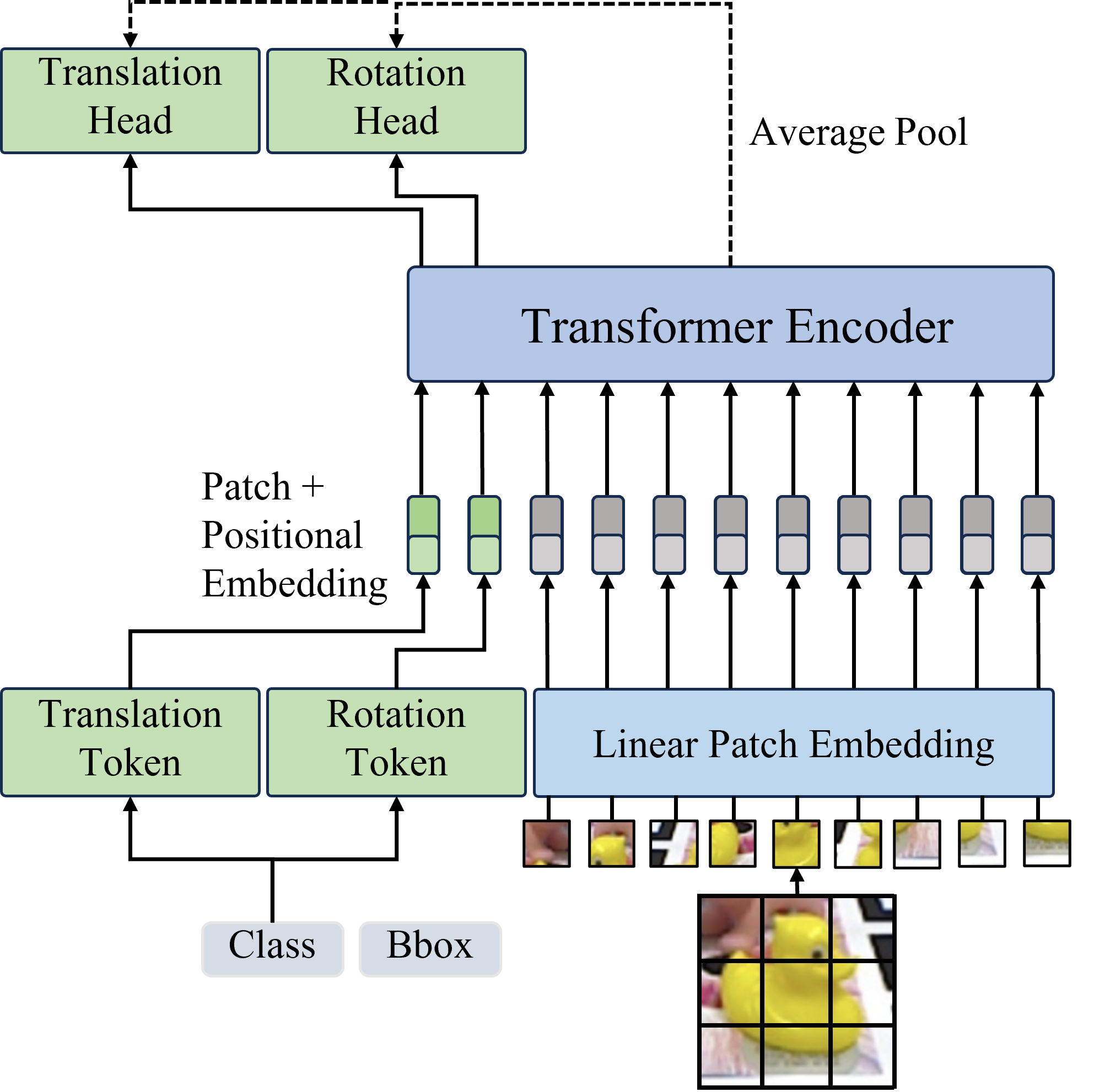
Figure 1: Illustration of modifying transformer-based image classification for direct pose regression. Rather than relying on a single class token or pooling the output features (indicated by the dotted arrow), we introduce two extra tokens for predicting rotation and translation. Optionally, the model can also be fed additional bounding box information.

The task of 6D pose estimation presents numerous challenges, mainly when dealing with scenes that are cluttered or suffer from occlusions. In these situations, predictive models often generate pose estimations without any associated measure of reliability. This lack of confidence indicators poses significant risks in practical applications like autonomous driving [30, 46], human-machine interfaces [31], and robotics [42, 16, 4], where incorrect predictions can lead to serious consequences. Solutions that offer confidence metrics often come with restrictions tied to specific frameworks or types of pose representation, such as keypoint detection [39, 10]. These constraints limit the adaptability of the methods and pose challenges for researchers attempting to incorporate confidence metrics into their own specialized tasks and models.

Current state-of-the-art techniques in 6D pose estimation have increasingly utilized similar advanced methods that use intricate intermediate features, such as keypoints and dense correspondences. This has resulted in significant improvements in accuracy, as seen in models like PVNet [33], GDRNet [45], and the latest ZebraPose [38]. Typically, these models adopt a simple feature extraction backbone based on the Resnet architecture [12]. This design decision is influenced by earlier studies, where larger or transformer-based networks were deemed computationally expensive for both training and real-time applications [8, 45]. However, this trade-off comes at the cost of diminished feature quality and predictive accuracy, leading to ongoing efforts to optimize architecture or employ more complex representations.

Additionally, these sophisticated techniques introduce their own set of challenges, such as limited adaptability in multi-modal scenarios and increased computational and time requirements, particularly when additional ground truth data has to be generated or real-time inference algorithms need to be optimized [29, 38].

Contrastingly, the foundational work in 6D pose estimation was relatively simple, mainly relying on direct regression techniques [2, 21]. The shift toward complexity is fueled by the challenging nature of accurately predicting 3D object poses, which involves both translational and rotational components. Initial implementations faced numerous issues, including finding the appropriate representation for rotation and translation, and designing efficient architectures and loss functions, all of which severely restricted performance and necessitated the development of more complex methods [45, 7].

This evolution has made the research landscape in 6D pose estimation distinctly different from traditional 2D computer vision tasks such as image classification, object detection, and human pose estimation. In these more established fields, direct regression-like methods have been quite effective and are generally considered the norm [8, 41, 27, 43, 34, 48].

In our investigation, we make a case for applying direct 6D pose regression within a modern context, incorporating proven pose representations, loss functions, and cutting-edge transformer-based network designs. We assert that this constitutes the new standard for fully learnable end-to-end methods, thus bridging the divide between classical 2D methodologies and the present advances in 6D pose estimation. Additionally, we demonstrate that linking the 3D Intersection-over-Union (3D-IoU) metric to the forecasted confidence, provides a straightforward and effective approach to extend many existing 6D pose estimation algorithms.

2 Related Work

Direct Pose Estimation. Posenet [22] pioneered using quaternions for predicting the rotation in camera pose estimation tasks. This approach brought a new dimension to the way rotations could be learned and represented. PoseCNN [47] took a multi-faceted approach by generating vectors that point towards the object center for each pixel to estimate translation. For rotation, they opted for direct regression using quaternions, similar to Posenet. SSD-6D [21] approached the problem by discretizing the viewpoint space and then classifying it. To estimate the object’s distance to the camera, they employed mask-based regression. CRT-6D [5] represents a more recent advancement by incorporating deformable attention modules. This method estimates the object’s pose, project keypoints onto the feature map, and then sample these to refine the initial pose prediction.

Indirect Pose Estimation. PVNet [33] introduced a two-stage method that initially estimates the 2D keypoints of objects in the image. These keypoints are then used in an uncertainty-driven Perspective-n-Point (PnP) algorithm to calculate the object’s pose. GDRNet [45], on the other hand, diverged from the use of sparse keypoints and instead employed dense correspondences. These dense correspondences encode the relationship between each image pixel and its corresponding point on the 3D model of the object. In a notable departure from traditional methods, GDRNet substituted the classical PnP algorithm with a neural network that directly regresses the pose from these dense correspondences. ZebraPose [38] also adopted a dense correspondence strategy but took a different route. In this approach, each pixel is classified into a binary class corresponding to a specific part of the object. This classification is then leveraged to match the image pixels with points on the object’s 3D model. Subsequently, a PnP algorithm is used to estimate the object’s pose.

Pose Confidence. The approach by Tekin et al. involves predicting the 2D projections of an object’s 3D bounding box and computing a score for each point based on its distance to the ground truth point. Extending this methodology, Gupta et al. predict 2D keypoints along with their confidence scores. These are then used to estimate object poses via an Efficient-PnP algorithm. The estimated poses enable the generation of masks and bounding boxes, which further refine the confidence scores through a Convolutional Neural Network (CNN) at processes both the mask and the Region of Interest (RoI).

3 Method

We aim to develop a 6D pose estimation technique that estimates the pose directly from an image, bypassing intermediary steps. However, in images with multiple objects, direct regression becomes ambiguous. To tackle this, we draw inspiration from previous works [45, 5, 38] and employ a two-step approach: initial object detection by an object detector, followed by separate pose estimation for each detected RoI. After the RoIs are extracted from the object detector, consistently with the recent studies [5, 45], we scale the RoIs by a factor of 1.2, crop them out, and resize the cropped image to a fixed size of 224x224 before using them as input for the network’s first layer.

Furthermore, we aim to separate the tasks of regressing the rotation and translation components of the pose. We specifically tailor the pose representation, loss functions, and network architecture to accomplish this.

3.1 Pose Representation

In the task of 6D pose estimation, particularly the prediction of the rotation $\mathbf{R}\in\text{SO}(3)$ and translation $\mathbf{t}\in\mathbb{R}^{3}$ using neural networks, the selection of an appropriate pose representation is a critical factor affecting the model’s performance [51]. Recent studies have shown the advantages of using a 6D rotation representation, denoted as $\mathbf{R}_{6\mathrm{d}}$, in excelling at 6D pose estimation tasks [45, 5, 19]. The 6D rotation representation $\mathbf{R}_{6\mathrm{d}}$ is defined as

$$\mathbf{R}_{6\mathrm{d}}=\left[\mathbf{r}_{1}\mid\mathbf{r}_{2}\right].$$ (1)

where $\mathbf{r}_{1},\mathbf{r}_{2}\in\mathbb{R}^{3}$ are the first two column vectors of the rotation matrix. The rotation matrix $\mathbf{R}$ can be recovered according to Gram-Schmidt orthonormalization. For rotational representation, we use the object-centric allocentric representation due to its equivariance with the RoI’s appearance [23].

Handling 3D translation in the camera’s coordinates is challenging because it is not linearly associated with pixel changes. To solve this, we adopt the method from Xiang et al., which decomposes translation into 2D centroid coordinates $\left(c_{x},c_{y}\right)$ and the object’s distance $t_{z}$ from the camera, simplifying 3D translation calculation via back-projection:

$$\mathbf{t}=K^{-1}t_{z}\left[c_{x},c_{y},1\right]^{T},$$ (2)

where $K$ denotes the camera’s intrinsic matrix.

Given that object detectors already supply an approximate 2D location of the object through the predicted bounding box center $\left(o_{x},o_{y}\right)$ and the network is only given the RoI to infer the pose, we employ the Scale-Invariant Translation Parameterization (SITP) for further refinement [26]. Specifically, we predict the offset between the object’s centroid and the bounding box center, normalized by the size of the bounding box. The SITP is then defined as $\mathbf{t}_{\mathrm{SITP}}=\left[\gamma_{x},\gamma_{y},\gamma_{z}\right]^{T}$, where

$$\left\{\begin{array}[]{l}\gamma_{x}=\left(c_{x}-o_{x}\right)/s\\ \gamma_{y}=\left(c_{y}-o_{y}\right)/s\\ \gamma_{z}=t_{z}/r\end{array}.\right.$$ (3)

Here, $s=\max(w,h)$ represents the size of the bounding box, and $r$ is the ratio of the image size $s_{\text{inp}}$ to the bounding box size, defined as $r=s_{\text{inp}}/s$.

However, the above representation is scale-agnostic, which means that the model cannot distinguish between a small object that is close to the camera and a large object that is far away. To address this issue, we introduce the Size Invariant Z Parametrization (SIZP). We utilize the back-projection formula (2) to derive:

$$t_{z}=\frac{f_{\text{s}}\cdot s_{\text{obj}}}{s}$$ (4)

where $f_{\text{s}}$ is the focal length of the camera, and $s_{\text{obj}}$ is the real-world size of the object along the $s$ direction. Notice that this approach is only viable if the object detector provides us with the class of the object. While the real-world size of the object, $s_{\text{obj}}$, is dependent on the object’s dimensions and is not precisely known due to rotation, we can approximate it using the object’s diameter $d$ and the fraction of the object’s diameter visible in the bounding box, denoted as $\gamma_{z}$. Consequently, the variable that our model aims to predict is formulated as

$$\gamma_{z}^{(\text{class})}=\frac{t_{z}}{r}=\frac{t_{z}\cdot s}{f_{s}\cdot d^{(\text{class})}}$$ (5)

As an extension of SITP, this representation provides a size-invariant description of the object’s translation. As demonstrated in our experiments, another benefit of this representation is that it scales the predicted variables for the translation to be in a similar range, which enhances the training stability without the need for further tuning.

3.2 Pose Tokens

For image classification tasks with vision transformers, Dosovitskiy et al. introduced the concept of class tokens, which are learnable embeddings that are appended to the feature map before feeding it into the transformer to aggregate context information for the classification task. For our tasks the class token provides two benefits. First by initializing the token with a learned embedding of the class from the object detector, we can aggregate class specific features. Second, we can use multiple tokens for different prediction tasks.

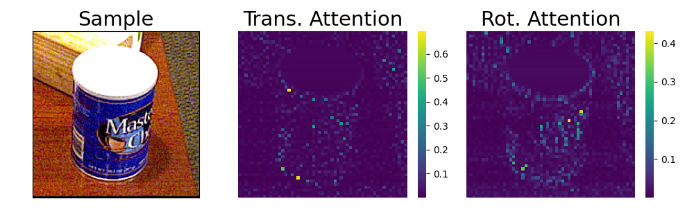
Figure 2: Visualization of the attention maps for a handpicked sample. Left the input image, in the middle the attention map of the translation token, and right the rotation token. To predict the rotation of the symmetric object, the rotation token needs to capture the label of the can.

Hence we further tailor the architecture to make it more conducive for 6D pose estimation tasks. We add two additional tokens to the network: one for aggregating the object’s translation and another for predicting its rotation features, see Fig. 1. The idea is to allow the model to learn different features for the rotation and translation prediction, as depicted by an example in Fig. 2. Lastly for predicting the pose, we use the pose tokens as input to two separate 3-layer Multi-Layer-Perceptrons (MLPs) to predict the rotation and translation individually.

3.3 Pose Confidence

Motivated by the contributions of Zhang et al., Tekin et al., we consider a method for assessing the reliability of the pose predictions. To obtain a ground truth score that our model aims to predict, we employ both the ground truth pose and the estimated pose to transform the 3D bounding box of the object and calculate the 3D-IoU. Even though straightforward, as shown by RT-SSD6D [39], the method becomes infeasible for dense object detectors or pose estimators due to the usually high number of predictions $\geq 100$ and the computational demand of the 3D-IoU [3]. However, the method gets enabled in the 2-stage setting since we need to calculate only one 3D-IoU per object detection. The 3D-IoU is then formulated as:

$$\text{IoU}_{3D}=\frac{\text{Volume of Intersection}}{\text{Volume of Union}}.$$ (6)

As illustrated in Fig. 3, the ground truth score quantifies the degree to which the predicted pose aligns with the actual ground truth pose.

However rather than predicting a single scalar score, we estimate a class-specific score, defined as:

$$\textbf{GT-Score}(c,p,\hat{p})=\hat{c}_{\text{scale}}\left(\text{IoU}_{3D}(c,\hat{p},p)\right)\cdot\textbf{OneHot}(c),$$ (7)

where $c$ denotes the object class, $p$ and $\hat{p}$ represent the ground truth and estimated poses, respectively, and $\hat{c}_{\text{scale}}$ serves as a scaling operator, treated as a hyperparameter, that scales the dimensions of the bounding box if the average translation error is much bigger than the original size of the objects. This method enhances class-specific detection, crucial for class-dependent representations like SIZP, see Eq. 5.

Lastly, our two-stage approach faces the issue of training on ground truth RoIs and classes, not accounting for object detector errors. We address this by using a denoising method inspired by Zhang et al., which involves injecting noise through false positives, either by changing the class randomly or removing the object from the RoI. This trains the model to handle detection inaccuracies.

Pred. Score: 0.90
GT Score: 0.89

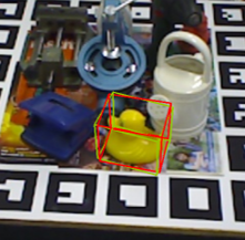
Pred. Score: 0.82
GT Score: 0.73

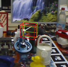
Pred. Score: 0.28
GT Score: 0.14

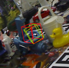
Pred. Score: 0.39
GT Score: 0.54

Figure 3: Visualization of predicted confidence score and ground truth 3D-IoU score. The green 3D bounding box depicts the box transformed with the ground truth pose, while the red box is transformed with the predicted pose. Below the imges the individual predicted scores and ground truth scores are shown.

3.4 Scene Complexity Conditioned Attention

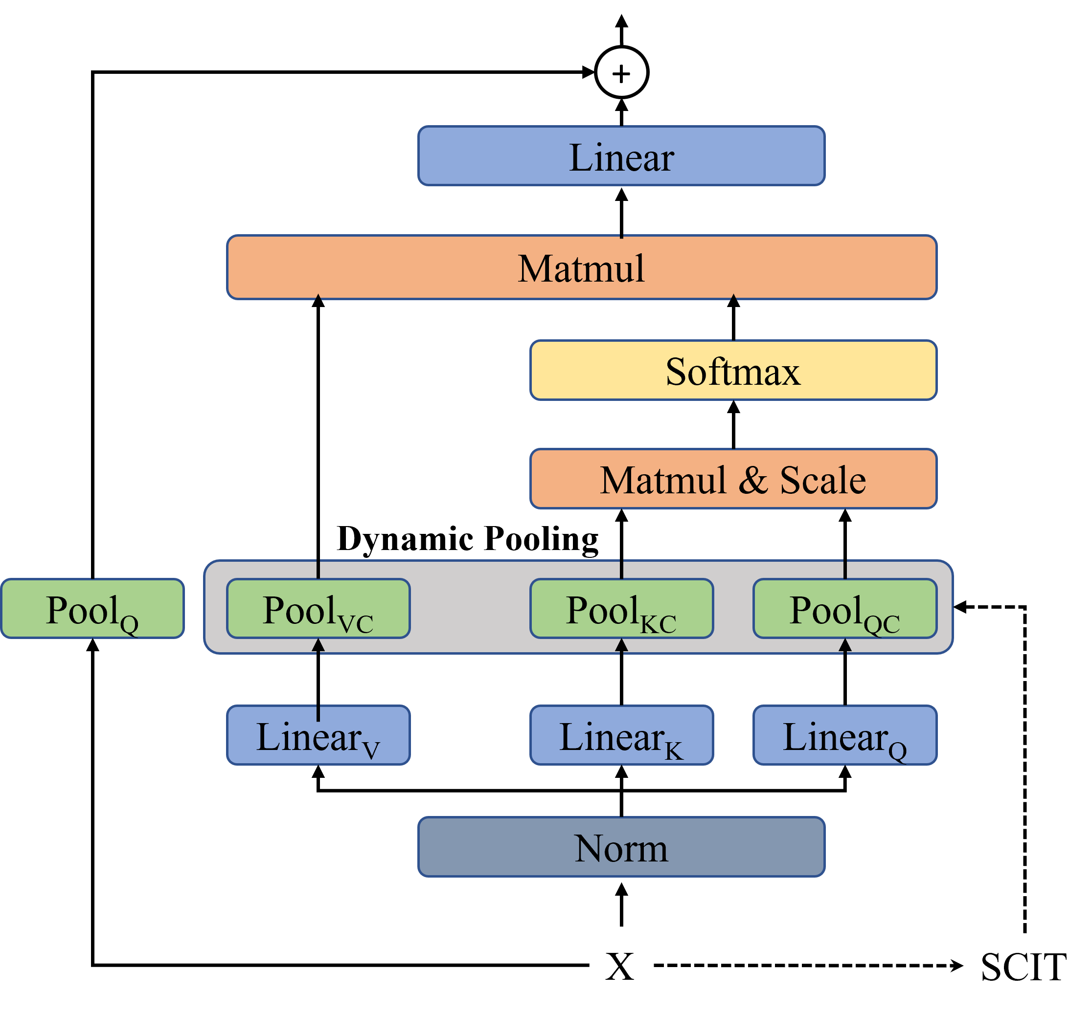
Figure 4: Depiction of the Scene-Complexity-Conditioned-Attention Mechanism. The SCIT is used as a condition for the pooling operations to extract the relevant features from the feature map, dependent on the scene context.

We base our architecture on the Multi-Scale-Vision-Transformer (MViT) [9, 25] that provides key improvements such as multiscale strategies adopted from classical CNNs and reduced sequence lengths via pooled attention. We further adapt the MViT architecture to our specific application by introducing a Scene-Complexity-Conditioned-Attention (SCCA) mechanism.

To account for variations in pose estimation accuracy caused by scene complexity and the challenges in predicting rotation and translation, we introduce the Scene Complexity Identifier Token (SCIT), denoted as $C_{\text{SCIT}}\in\mathbb{R}^{D}$. We design this token to condense relevant features from the feature map according to the scene’s context, helping filter out extraneous or misleading feature elements by using it to predict the pose confidence.

We formalize our attention mechanism as follows: Consider an input feature map $X\in\mathbb{R}^{H\times W\times D}$, and define the linear projections $W_{Q},W_{K},W_{V}\in\mathbb{R}^{D\times D}$. The feature map is then transformed by the pooling operators $\mathcal{P}_{Q}$, $\mathcal{P}_{K}$, and $\mathcal{P}_{V}$, which are applied after the projections as:

$$\tilde{Q}=\mathcal{P}_{Q}(XW_{Q}),\ \tilde{K}=\mathcal{P}_{K}(XW_{K}),\ \tilde{V}=\mathcal{P}_{V}(XW_{V}),$$

yielding reduced-dimensionality maps $\tilde{Q},\tilde{K},\tilde{V}\in\mathbb{R}^{\tilde{H}\times\tilde{W}\times D}$ with $\tilde{H}\leq H$ and $\tilde{W}\leq W$, as illustrated in Fig. 4.

We also integrate a standard convolutional pooling operation, $\mathcal{P}_{Q}$, serving as a residual connection for the input feature map. As depicted in Fig. 5, the pooling operations are conditioned on the SCIT vector in two distinct methodologies. Firstly, we apply a dynamic filter convolution [20] defined by: $\mathcal{K}_{Q}=\text{Linear}_{Q_{C}}(C_{\text{SCIT}}),$ where $\mathcal{K}_{Q}\in\mathbb{R}^{D\times D\times k_{h}\times k_{w}}$. The corresponding conditional pooling operator, $\mathcal{P}_{Q_{C}}$, is:

$$\mathcal{P}_{Q_{C}}(Q) =\text{Conv}_{\mathbf{s,p}}(Q,\mathcal{K}_{Q})=\tilde{Q},$$

with $Q=XW_{Q}\in\mathbb{R}^{H\times W\times D}$, and stride and padding parameters denoted by $\mathbf{s}=(s_{h},s_{w})$ and $\mathbf{p}=(p_{h},p_{w})$, respectively.

Secondly, we utilize a cross-attention mechanism [44]. During the forward pass, attention weights are computed using

$$A=\text{Softmax}(\sum_{i=1}^{D}\left(\text{Linear}_{Q_{C}}(C_{{\text{SCIT}}})_{i}\cdot Q_{i}\right)\cdot\alpha),$$

with $\alpha$ being a scaling factor. The attended feature map, $Q_{\text{attended}}=Q\cdot A$, is processed to obtain $\tilde{Q}=\text{Conv}_{\mathbf{s,p}}(Q_{\text{attended}})$ with learned weights. And similar of course for $\mathcal{P}_{K_{C}}$ and $\mathcal{P}_{V_{C}}$. Ultimately, the attention mechanism is calculated as:

$$Z =\text{Attn}(Q,K,V)=\text{Softmax}\left(\frac{\tilde{Q}\tilde{K}^{T}}{\sqrt{D}}\right)\tilde{V}.$$

Lastly we use three different models with scales, Small, Base, and Large, which we denote as PViT-6D-s, PViT-6D-b, and PViT-6D-l. For simplicity and comparability, we use the same model configurations as in MViTv2 [25].

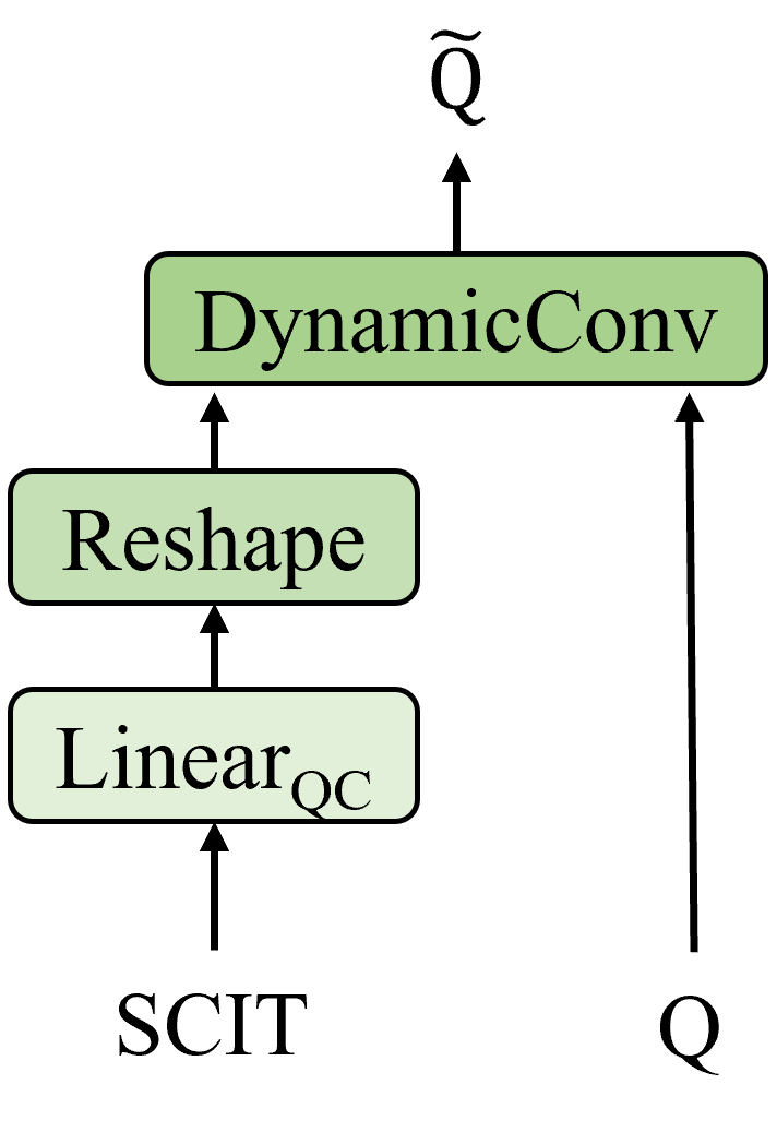
(a) Dynamic-Filter

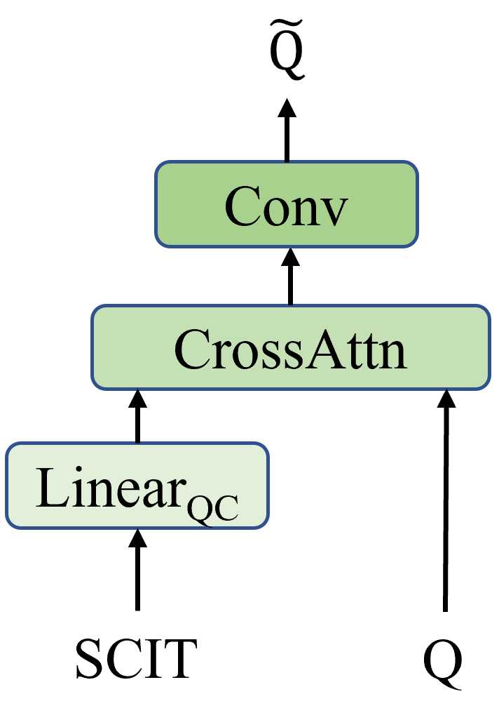
(b) Cross-Attention

Figure 5: Scene-Complexity-Pooling Module: (a) Dynamic Convolution based, the SCIT is used to generate weights for the Convolution, (b) right cross-attention based pooling, the SCIT is used to generate attention maps, which are then used to pool the feature map with a learned convolution.

3.5 Loss Function

In addressing the pose loss, we adhere to the same loss function that has been employed in numerous recent works[45, 5, 6, 47], which have demonstrated notable success. Drawing inspiration from Simonelli et al., we decouple the rotation and translation loss. Consequently, the pose loss is defined as follows: $\mathcal{L}_{\text{Pose}}=\lambda_{\text{c}}\mathcal{L}_{\text{centroid}}+\lambda_{z}\mathcal{L}_{z}+\lambda_{\mathbf{R}}\mathcal{L}_{\mathbf{R}}$, where

$$\left\{\begin{array}[]{l}\mathcal{L}_{\text{center}}=\left\|\left(\hat{\gamma}_{x}-{\gamma}_{x},\hat{\gamma}_{y}-{\gamma}_{y}\right)\right\|_{1},\\ \mathcal{L}_{z}=\left\|\hat{\gamma}_{z}-{\gamma}_{z}\right\|_{1},\\ \mathcal{L}_{\mathbf{R}}=\underset{\mathbf{x}\in\mathcal{M}}{\operatorname{avg}}\left\|\hat{\mathbf{R}}\mathbf{x}-{\mathbf{R}}\mathbf{x}\right\|_{1}\end{array}\right.$$ (11)

Here $\left|\left|\cdot\right|\right|_{1}$ denotes the $L1$-norm and $\mathcal{M}$ is the model of the predicted object. The $\lambda$-s are used as hyperparameters to weight the different losses. The loss for the rotation is a variant of the pose matching loss [47], where only the rotation is used to transform the points. For objects with symmetrical characteristics, we employ a symmetry-aware pose loss as used by Wang et al. This loss is defined as $\min_{\mathbf{R}\in\mathcal{R}}\mathcal{L}_{\mathbf{R}}(\hat{\mathbf{R}},\mathbf{R})$. Here, the loss function takes into account the object’s inherent symmetries to determine the rotation closest to the ground truth rotation. In this equation, $\mathcal{R}$ represents the set of all feasible ground truth rotations that conform to the object’s symmetry.

For the class loss we opt for a simple cross entropy loss:

$$\mathcal{L}_{\text{cls}}(c,\hat{s},p,\hat{p}) =\mathcal{L}_{\text{cls}}(c,\hat{s},\text{IoU}_{3d})$$ (12)

$$=-\sum_{i=1}^{N}\textbf{GT-Score}_{i}\log(\hat{s}_{i})$$ (13)

4 Experiments

In this section, we delve into the specifics of the experiments. We begin by outlining the datasets and evaluation criteria employed. Subsequently, we conduct ablation studies. We conclude by comparing our findings with those obtained using state-of-the-art approaches on both the LM-O [1] and YCB-V [47] datasets and investigate the effectiveness of the pose confidence.

4.1 Datasets

The Linemod (LM) [13] dataset comprises 15 scenes, each with around 1,200 images and a single annotated object, providing ground truths like 3D models, bounding boxes, masks, and 6D object poses [13]. Due to high accuracy achieved by various methods [47, 38, 45, 26], research has pivoted to the more challenging LM-O dataset [1], which adds a test set with 1,214 images and an average of eight occluded objects per image. We leverage the LM and the BOP challenge’s PBR datasets, the latter containing 50 scenes with approximately 1,200 rendered images each [15], to enhance pose estimation model performance [45, 37].

Furthermore, our experiments extend to the YCB-V dataset [47], with 21 objects across 92 video-recorded scenes, presenting heavier occlusions and intricate symmetries, backed by over 100,000 real images and additional PBR data from the BOP challenge [15] for training.

4.2 Evaluation Metrics

For the evaluation of the pose estimation, we employ the commonly used ADD(-S) metric [14]. The ADD(-S) metric consists of the ADD metric, which is defined to be the average distance between the 3D points after transforming them with the predicted and ground truth pose. For symmetric objects, we use the ADD-S metric, which is defined to be the minimal distance between the points after transforming them. For LM-O, we use the average recall (AR) of the ADD(-S) metric, where a true pose is given when the prediction has an ADD(-S) score below a certain threshold. Other works [38, 45] have used a threshold of 10% of the object’s diameter, which we also use in our experiments.

Additionally, for the YCB-V dataset, we also report the area under the curve (AUC) of the ADD(-S) metric, where the threshold is varied in the interval [0, 10cm] [47].

4.3 Implementation Details

The implementation of the model is done using PyTorch [32], and it is trained across three Nvidia 3080Ti GPUs. We employ the AdamW optimizer [28] with a learning rate set to 1.2e-4 and a batch size configured to 192. We use a linear learning rate scheduler, incorporating a 2-epoch warm-up phase. Additionally, we set the weight decay to 1e-4, and the gradient norms are clipped at 0.1. The training lasts 150 epochs, with early stopping with a patience set to 15. For image augmentation, we apply random adjustments in brightness, contrast, saturation, hue, coarse dropout, and color jitter. In terms of bounding box augmentation, we perform uniform scaling and shifting by 10% and 35% of the original size, respectively.

4.4 Ablation Study

To test changes, we implement an ablation dataset. We use the LM dataset with an additional ten scenes from the PBR dataset to test on the LM-O dataset. We call this dataset LM-O-A.

Influence of z-representation.

To test the absolute z-representation, we incorporate a bounding box embedding with the token embeddings. Our findings reveal the model’s difficulty in accurately predicting the absolute z-coordinate with 54.6% ADD(-S) accuracy, while the relative z-coordinate(SITP) and our proposed representation(SIZP) achieve, in comparison, higher accuracies of +6.5% and +7.2%, respectively.

Influence of Class Refinement. Further, we investigate the influence of the class refinement. In a test scenario where we disturb 20% of the ground-truth classes, the refinement model recovers the correct class in 92.9%, and with our denoising strategy 94.7% of the cases. We compare the model’s performance with and without class refinement, utilizing the SIZP representation. We see a slight increase of +0.2% ADD(-S) accuracy when using Faster-RCNN detections from Ren et al..

Dependency on Encoder Architecture. We want to investigate the influence of the encoder architecture on the performance of the model. We use a standard vision transformer as a baseline ViT-B/16 [8] and multiple versions of the MViTv2 [25] architecture. MViTv2-s, MViTv2-b, MViTv2-l, with varying depth and parameter count. We also add one convolutional-based backbone ResNet-50 [12] for a comparison, where we average pool the output feature map.

Model	ADD(-S)	GFLOPs	Param (M)
ResNet-50*	43.1	4.3	25.6
ViT-B/16	62.7	17.7	86.4
MViTv2-s	56.9	7.1	29.8
MViTv2-b	62.0	10.4	44.9
MViTv2-l	65.2	42.9	201.2

Table 1: Dependency on the Encoder Architecture. Depicted are Encoder-Architecture, GLFOPS and parameter count in million. * means no tokens are used, ADD(-S) accuracy reported on LM-O-A.

The results depicted in Tab. 1 show, that the MViTv2 architecture scales well with the number of parameters and provides a better speed-accuracy tradeoff than the ViT architecture, by only having -0.7% accuracy with only 52% the amount of parameters.

Pose Token Ablation. To test the effectiveness of using two tokens for translation and rotation, we also experiment with using a single pose token. To have a fair comparison with the pool baseline, we concatenate the pooled output feature vector with a learned class embedding. We find that using a single pose token for both translation and rotation already achieves an improvement of +3.2% over the pool baseline with 57.4% accuracy compared to 60.6%. Additionally, segregating pose tokens for translation and rotation enhances performance by an additional +1.4% over using a single token, suggesting the model’s ability to distill distinct features for each.

Influence of SCCA. For comparing the effectiveness of the SCCA from Sec. 3.4, we use the base pose token version, with and without the cross-attention- and the convolution-based SCCA. Furthermore, we investigate the effects of using the conditioned pooling only on the queries.

Variant	ADD(-S)	$\Delta$GFLOPs	Param (M)
None	62.0	10.3	51.8
Convq	-0.2	+0.1	53.8
Attnq	+0.5	+0.2	52.2
Convq,k,v	+0.0	+0.4	57.7
Attnq,k,v	+0.4	+1.0	53.1

Table 2: Comparison of SCCA-versions. GFLOPs are reported as difference from the Pool-version. ADD(-S) accuracy reported on the LM-O-A dataset

Tab. 2 indicates that while the convolutional-based SCCA does not enhance model performance despite more parameters, the attention-based SCCA improves it by +0.5% with minimal parameter and computational increase. Additionally, applying conditioned pooling solely to queries is more effective than on keys and values in terms of accuracy and computational efficiency.

4.5 Comparison with State of the Art

For evaluating LM-O, we employ FasterRCNN detections, which are publicly accessible [35] and also conduct evaluations using the FCOS [40] detections supplied by Su et al.. We observe an increase of +1.1% in accuracy (from 71.2% using PViT-6D-b) by going from FasterRCNN to FCOS detections, which is in line with the results of Su et al.. For assessments on the YCB-V dataset, we leverage the FCOS detections made available by CDPNv2 [26].

As shown in Tab. 3, our smallest model PViT-6D-s model is on par with methods like GDRNet [45], SOPose [6]. Moreover, we outperform the current state-of-the-art pose estimation model ZebraPose [38] by +0.3% on the LM-O dataset, and +3.3% on the YCB-V dataset, with our largest version, PViT-6D-l, utilizing the same FCOS detections. Notably, PViT-6D-l, despite having over seven times more parameters than ZebraPose, effectively infers poses for all classes. On YCB-V, PViT-6D-l shows a +2.7% improvement over ZebraPose, and excels in symmetric objects accuracy by an average of +19%, as detailed in appendix.

Model	PVNet [33]	GDRNet [45]	SO-Pose [6]	CRT-6D[5]	ZebraPose [38]	Ours(-s)	Ours(-b)	Ours(-l)
N	8	8	1	1	8	1	1	1
Params(M)	-	28.8	-	-	28.9	31.8	52.2	213.6
Ape	15.8	46.8	48.4	53.4	57.9	43.3	58.6	60.6
Can	63.3	90.8	85.8	92.0	95.0	91.8	96.0	97.4
Cat	16.7	40.5	32.7	42.0	60.6	44.1	56.4	60.0
Driller	65.7	82.6	77.4	81.4	94.8	88.8	93.3	95.8
Duck	25.2	46.9	48.9	44.9	64.5	56.5	58.3	66.0
Eggbox*	50.2	54.2	52.4	62.7	70.9	47.5	62.3	68.4
Glue*	49.6	75.8	78.3	80.2	88.7	75.4	84.6	85.9
Holepuncher	36.1	60.1	75.3	74.3	83.0	57.0	75.5	83.9
Average	40.8	62.2	62.3	66.3	76.9	63.1	72.3	77.3

Table 3: Comparison with the State of the Art on LM-O. We report the Average Recall (%) of ADD(-S). N is the number pose estimators for the dataset. In the case of LM-O $N_{\text{max}}=8$. ($\ast$) denotes symmetric objects and “-” denotes unavailable results.

Method	N	ADD(-S)	AUC of ADD(-S)
PVNet[33]	21	-	73.4
GDRNet[45]	21	60.1	84.4
SO-Pose[6]	1	56.8	83.9
CRT-6D[5]	1	72.1	87.5
Zebra[38]	21	80.5	85.3
Ours(-b)	1	77.3	83.7
Ours(-l)	1	83.2	85.6

Table 4: Comparison with State of the Art on YCB-V. Reported are Average Recall of ADD(-S) (%) and the AUC of the ADD(-S).

4.6 Confidence Analysis

To evaluate the effectiveness of the pose confidence from Sec. 3.3, we visualize both predicted confidence scores and ground truth 3D-IoU scores in Fig. 6. We notice a pattern of concentration around higher IoU scores, consistent with our ADD(-S) value of 72.3% with PViT-6D-b, see Tab. 3. However, the scores exhibit a significant degree of variance, indicating the challenges in predicting them accurately. It is crucial to clarify that the objective is not to predict the 3D-IoU score precisely. Instead, the aim is to establish a relationship between poses that are easier to predict and those that are more challenging.

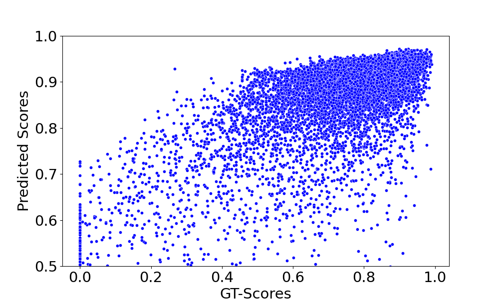
Figure 6: Predicted classification scores and ground truth IoU scores visualized in a scatter plot with classification scores of  0.5, resulting in a Spearman’s coefficient $\rho=0.71$.

To further analyze the effectiveness of the pose confidence, we visualize the predicted confidence and ground truth 3D-IoU scores with respect to the ADD(-S) metric in meters, see Fig. 7, resulting in a steady decrease in pose error.

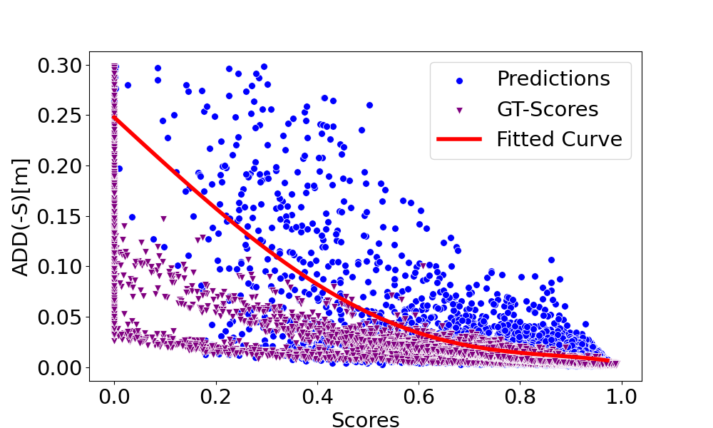
Figure 7: Scatter plot of ADD(-S) error in meters and scores. Shown are the ground truth classification scores and predicted scores in a scatter plot. Additionally shown is polynomial fit of the predicted scores of degree 10.

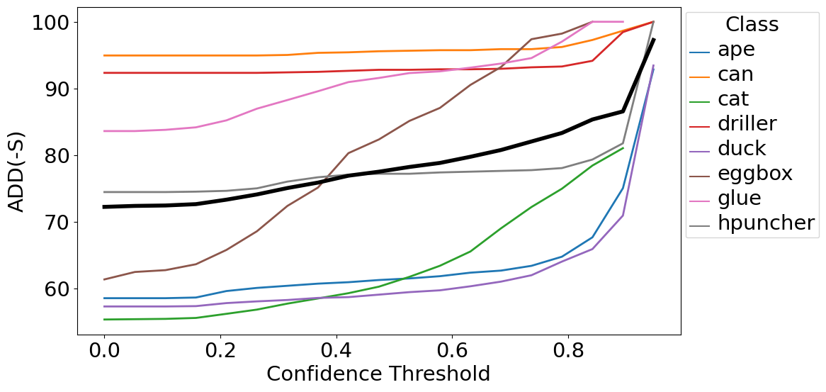
Figure 8: Plotted curves of predicted confidence scores and ADD(-S) accuracy for each class. In black is the mean curve.

In Fig. 8, we explore the relationship between class, confidence levels, and the accuracy of ADD(-S) measurements. We observe a gradual ascent in precision for specific objects due to inherent high precision for these objects and the only few incorrect low-confidence predictions, which aligns with our expectations. There is a notable upward trend in accuracy corresponding to the application of stricter confidence thresholds. This trend and the beforementioned results suggests that pose confidence is a reliable predictor of pose estimation accuracy.

4.7 Runtime Analysis

The assessment was conducted on a system equipped with a GTX1080Ti and an Intel i7-6850K CPU @ 3.60GHz. We evaluated the accuracy and the inference latency for different object counts and model sizes. The CRT-6D value is taken from [5] and was measured on a similar setup.

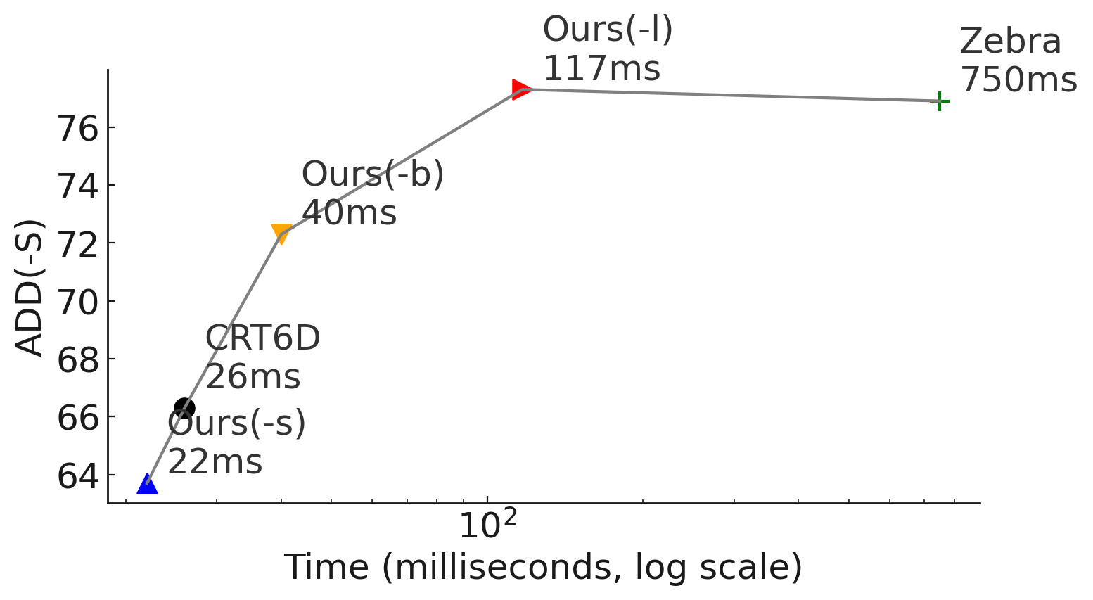
Figure 9: Inference Time Analysis on YBC-V with $\sim 4$ objects, excluding object detection. Shown is the ADD(-S) against the inference time in [ms].

PViT-6D-s exhibits slight advantage in speed while outperformed by CRT-6D[5] in accuracy. Zebrapose[38], in our configured environment, required 188ms to process a single object. So our largest model not only outperforms the state-of-the-art in accuracy but also in speed.

5 Conclusion

In conclusion, in our study, we demonstrated the viability of using direct regression for pose estimation by using specialized pose tokens, yielding both robust results and high performance. Additionally, we succeeded in learning a measure of pose confidence that is an effective indicator of the model’s certainty of a prediction. For future research, we aim to implement this method in a multi-modal setting, where pose estimation is a subset of the model’s capability.

Appendix A Influence of Padding Information

To evaluate whether we can reduce the amount of redundant information we feed into the model, we investigate an alternative to squaring the bounding box, which might potentially introduce confusing information by showing parts of other objects in occluded scenes. Instead of squaring, we crop the image precisely to the bounding box and pad it into a square shape using zero padding. As it turns out, on LM-O-A, see Sec. 4, there is no benefit in this approach, resulting in a decrease in average recall of ADD(-S) by 0.1%.

Appendix B BOP Results

We train PViT-6D-b/l, under the BOP-setup [15] on the YCB-V [47] and LM-O [1] datasets and compare them to the previously examined state-of-the-art methods and the two overall top-performing methods, GDRNPP and GPose, based on GDRNet [45], and ZebraSAT, based on ZebraPose [38] on the BOP-Leaderboard with the highest core average recall for RGB-only prediction. Additionally we take the best-performing method on YCB-V and LM-O individually, namely CosyPose [24] and RADet building on the work of Hai et al., Hu et al.. We use the detections from CDPNv2 [26] for comparability. Unlike before, now we use only PBR data for training on LM-O and evaluate only on a set of selected keyframes. We uploaded the predictions to the BOP-Website, where the results are evaluated and submitted under the name PViT-6D. We show in Tab. 5 and Tab. 6 the results competitive results of our method on LM-O and YCB-V, respectively.

Method	$AR_{MSPD}$	$AR_{MSSD}$	$AR_{VSD}$	$AR$
CRT-6D [5]	83.7	64.0	50.4	66.0
Zebra [38]	88.0	72.1	55.2	71.8
GDRNPP	88.7	70.1	54.9	71.3
ZebraSAT	88.9	73.6	56.2	72.9
GPose	87.9	68.3	53.6	69.9
RADet	87.7	76.1	59.7	74.5
Ours(-b)	87.7	75.3	58.8	73.0
Ours(-l)*	88.8	79.2	62.0	76.7

Table 5: Results on the LM-O dataset under BOP setup [15]. GDRNPP, ZebraSAT, GPose are the current overall top-performing methods in the BOP-challenge. And RADet the top-performing method on LM-O. The results are obtained from the BOP-Leaderboard. (*) PViT-6D-l has been trained on PBR and real data.

Method	$AR_{MSPD}$	$AR_{MSSD}$	$AR_{VSD}$	$AR$
CRT-6D [5]	77.4	77.6	70.6	75.2
Zebra [38]	86.4	83.0	75.1	81.5
GDRNPP	86.9	84.6	76.0	82.5
ZebraSAT	87.2	84.2	77.0	83.0
GPose	85.3	83.0	78.3	82.4
CosyPose	88.0	88.5	79.5	85.3
Ours(-b)	84.0	84.4	75.4	81.3
Ours(-l)	85.7	87.1	76.9	83.2

Table 6: Results on the YCB-V dataset under the BOP-setup [15]. GDRNPP, ZebraSAT, GPose are the current overall top-performing methods in the BOP-challenge and CosyPose [24], the best-performing method on YCB-V. The results are obtained from the BOP-Leaderboard.

Appendix C Detailed Results on YCB-V

In Tab. 7, we present the detailed results on the YCB-V dataset [47], w.r.t. ADD(-S) metric. We compare our method to other state-of-the-art methods. We show that our method PViT-6D-l outperforms the current state-of-the-art method ZebraPose [38] in terms of average recall of ADD(-s).

Object	Single-Stage [17]	GDR-Net [45]	CRT6D [5]	ZebraPose [38]	Ours(-b)	Ours(-l)
002_master_chef_can	-	41.5	-	62.6	27.4	28.7
003_cracker_box	-	83.2	-	95.5	84.3	90.3
004_sugar_box	-	91.5	-	96.3	94.8	100.0
005_tomato_soup_can	-	65.9	-	80.5	89.3	94.9
006_mustard_bottle	-	90.2	-	100.0	95.7	98.9
007_tuna_fish_can	-	44.2	-	70.5	69.2	70.4
008_pudding_box	-	2.8	-	99.5	84.6	85.1
009_gelatin_box	-	61.7	-	97.2	67.3	79.0
010_potted_meat_can	-	64.9	-	76.9	70.2	69.5
011_banana	-	64.1	-	71.2	78.7	92.6
019_pitcher_base	-	99.0	-	100.0	100.0	100.0
021_bleach_cleanser	-	73.8	-	75.9	81.2	88.1
024_bowl*	-	37.7	-	18.5	85.5	99.5
025_mug	-	61.5	-	77.5	81.0	93.9
035_power_drill	-	78.5	-	97.4	94.7	97.2
036_wood_block*	-	59.5	-	87.6	72.9	99.9
037_scissors	-	3.9	-	71.8	43.8	56.3
040_large_marker	-	7.4	-	23.3	21.1	27.0
051_large_clamp*	-	69.8	-	87.6	97.3	98.3
052_extra_large_clamp*	-	90.0	-	98.0	92.5	93.8
061_foam_brick*	-	71.9	-	99.3	99.0	99.6
Average	53.9	60.1	72.5	80.5	77.3	83.2

Table 7: Detailed Results on YCB-V: Reported is the Average Recall of ADD(-S) in %. (*) denotes symmetric objects, (-) denotes the results are not reported in the literature.

Appendix D Visual Examples of Attention Maps

Further examples of attention maps for different objects are shown in Fig. 10. The first column shows the sample RoI image. The first row shows the rotation attention map, and the second row shows the translation attention map. The columns depict the different stages of the model. We visualize one random example from the LM-O dataset for each object.

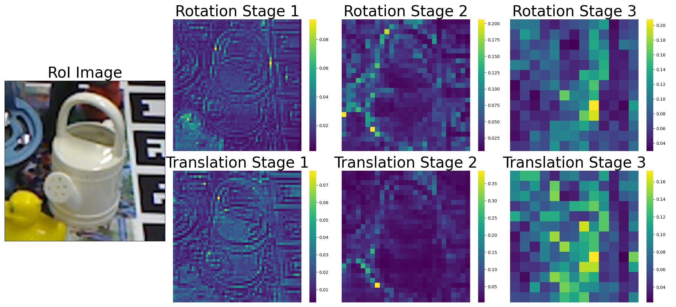
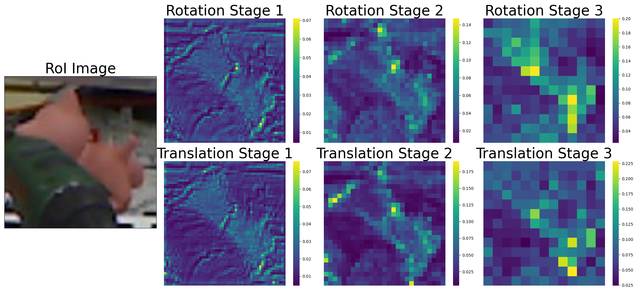
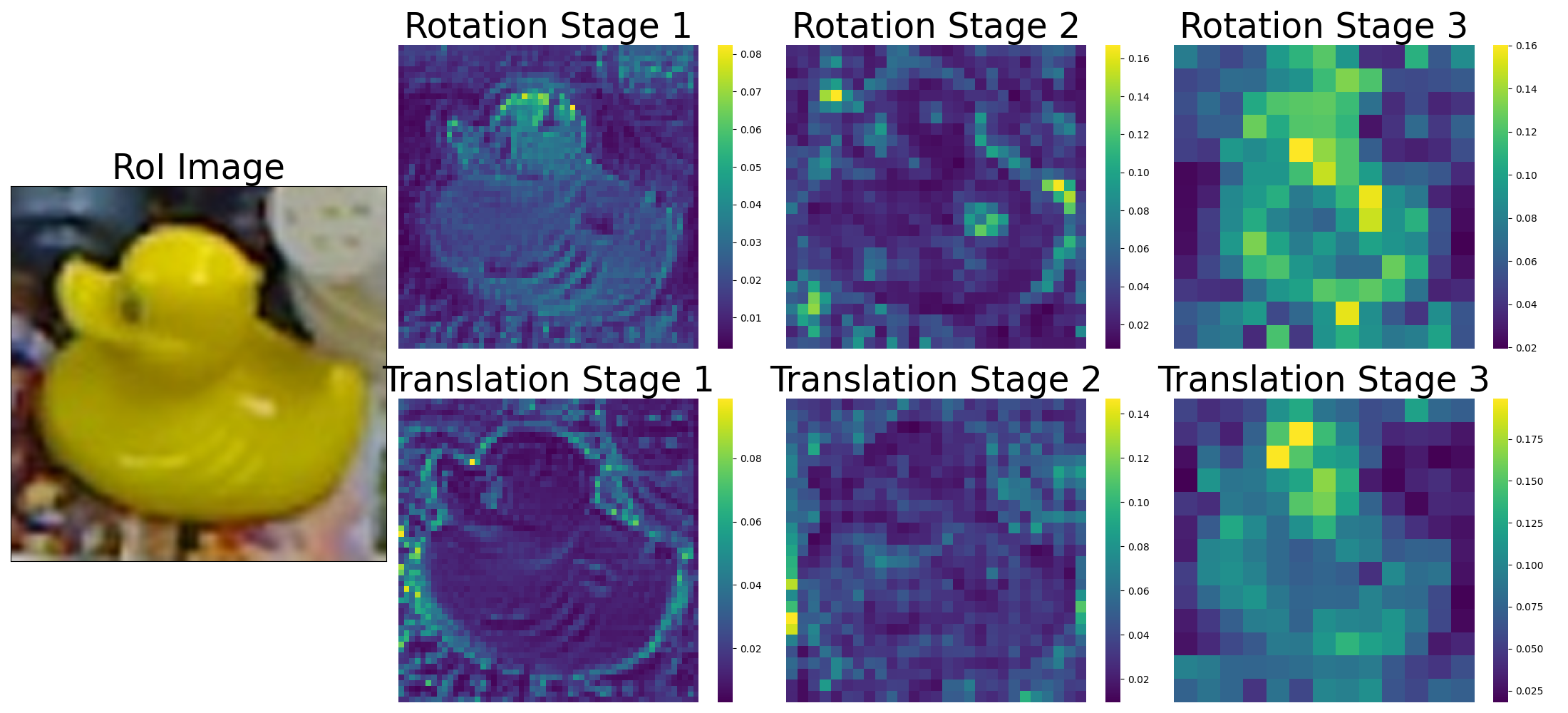
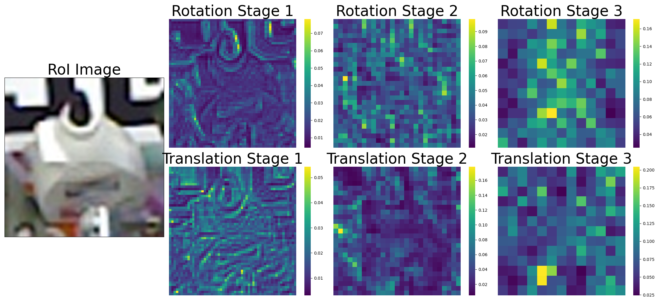
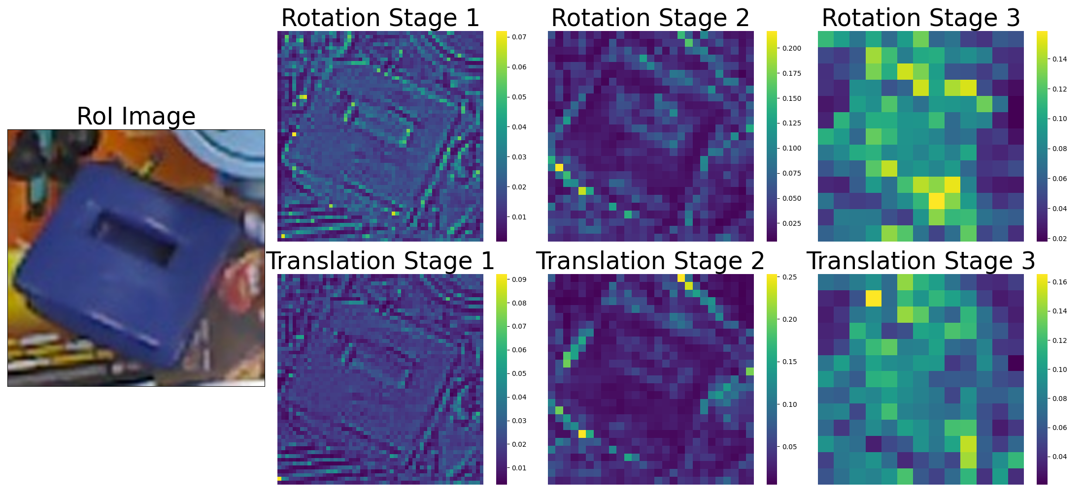
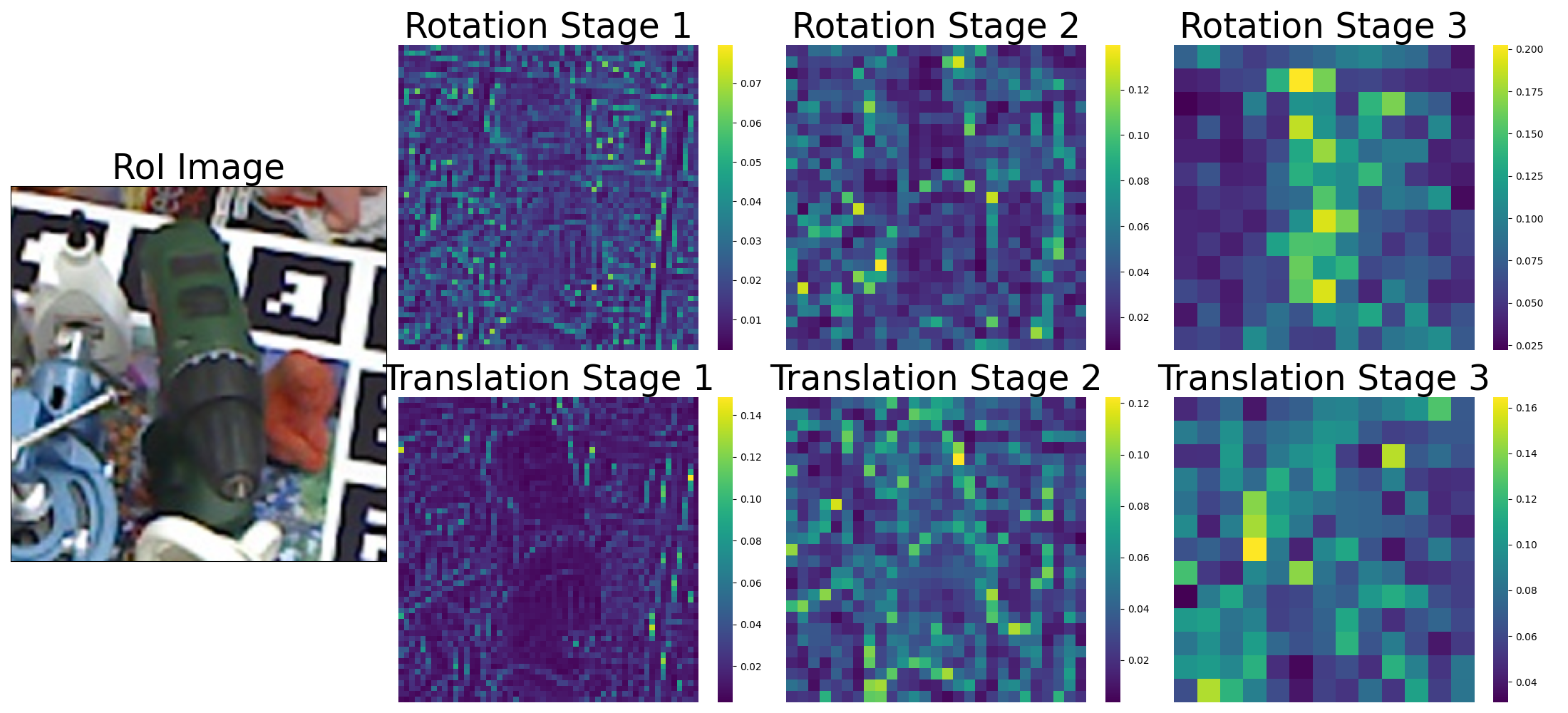
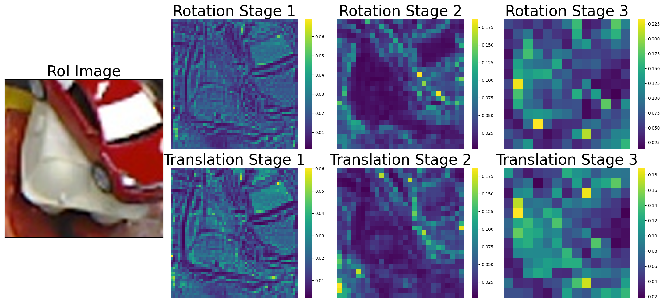
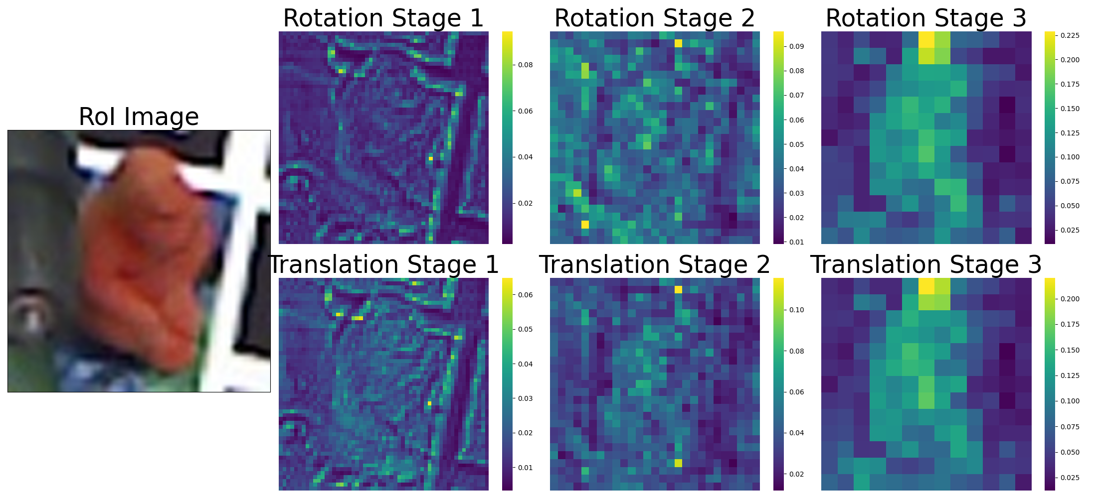
Figure 10: Attention maps for different objects of the LM-O dataset. The top row depicts the rotation attention, and the bottom row shows the translation attention. The columns depict the different stages of the transformer.

Appendix E Late Fusion Saliency Map

When using the Pool version, see Fig. 1, we appended the class and bounding box embedding to the pooled feature map. To demonstrate the impact of this modification, we present a saliency map of this feature vector, focusing on its relation to the pose loss. As indicated in Fig. 11, we observe that the saliency of the second last row, the bounding box embedding, is significantly lower compared to the feature vector and the class embedding. This outcome aligns with our expectations as the pose representation is designed to be unaffected by variations in the bounding box. Conversely, the class embedding plays a crucial role in the prediction process, as indicated by the high saliency in the last row.

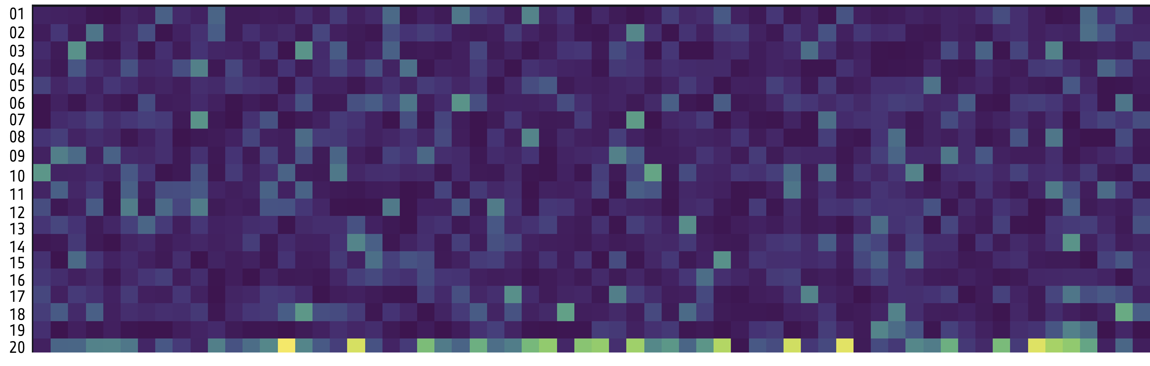
Figure 11: Saliency Map of Pooling-Version. The saliency map for the late fusion of class and bounding box embeddings is structured as follows: The initial 18 rows depict the 1152-dimensional pooled feature vector. The second last row represents the bounding box embedding, and the final row is dedicated to the class embedding. This visualization is based on the mean values derived from a batch of 1000 random samples.

References

- Brachmann et al. [2014] Eric Brachmann, Alexander Krull, Frank Michel, Stefan Gumhold, Jamie Shotton, and Carsten Rother. Learning 6d object pose estimation using 3d object coordinates. In European Conference on Computer Vision, 2014.
- Bui et al. [2018] Mai Bui, Sergey Zakharov, Shadi Albarqouni, Slobodan Ilic, and Nassir Navab. When regression meets manifold learning for object recognition and pose estimation. 2018 IEEE International Conference on Robotics and Automation (ICRA), pages 1–7, 2018.
- Carion et al. [2020] Nicolas Carion, Francisco Massa, Gabriel Synnaeve, Nicolas Usunier, Alexander Kirillov, and Sergey Zagoruyko. End-to-end object detection with transformers. ArXiv, abs/2005.12872, 2020.
- Castro et al. [2017] Mario Di Castro, Jorge Camarero Vera, Manuel Ferre, and Alessandro Masi. Object detection and 6d pose estimation for precise robotic manipulation in unstructured environments. In International Conference on Informatics in Control, Automation and Robotics, 2017.
- Castro and Kim [2023] Pedro Castro and Tae-Kyun Kim. Crt-6d: Fast 6d object pose estimation with cascaded refinement transformers. In 2023 IEEE/CVF Winter Conference on Applications of Computer Vision (WACV), pages 5735–5744, 2023.
- Di et al. [2021] Yan Di, Fabian Manhardt, Gu Wang, Xiangyang Ji, Nassir Navab, and Federico Tombari. So-pose: Exploiting self-occlusion for direct 6d pose estimation. 2021 IEEE/CVF International Conference on Computer Vision (ICCV), pages 12376–12385, 2021.
- Do et al. [2018] Thanh-Toan Do, Trung T. Pham, Mingpeng Cai, and Ian D. Reid. Lienet: Real-time monocular object instance 6d pose estimation. In British Machine Vision Conference, 2018.
- Dosovitskiy et al. [2020] Alexey Dosovitskiy, Lucas Beyer, Alexander Kolesnikov, Dirk Weissenborn, Xiaohua Zhai, Thomas Unterthiner, Mostafa Dehghani, Matthias Minderer, Georg Heigold, Sylvain Gelly, Jakob Uszkoreit, and Neil Houlsby. An image is worth 16x16 words: Transformers for image recognition at scale. ArXiv, abs/2010.11929, 2020.
- Fan et al. [2021] Haoqi Fan, Bo Xiong, Karttikeya Mangalam, Yanghao Li, Zhicheng Yan, Jitendra Malik, and Christoph Feichtenhofer. Multiscale vision transformers. 2021 IEEE/CVF International Conference on Computer Vision (ICCV), pages 6804–6815, 2021.
- Gupta et al. [2019] Kartik Gupta, Lars Petersson, and Richard I. Hartley. Cullnet: Calibrated and pose aware confidence scores for object pose estimation. 2019 IEEE/CVF International Conference on Computer Vision Workshop (ICCVW), pages 2758–2766, 2019.
- Hai et al. [2023] Yang Hai, Rui Song, Jiaojiao Li, Mathieu Salzmann, and Yinlin Hu. Rigidity-aware detection for 6d object pose estimation. 2023 IEEE/CVF Conference on Computer Vision and Pattern Recognition (CVPR), pages 8927–8936, 2023.
- He et al. [2015] Kaiming He, X. Zhang, Shaoqing Ren, and Jian Sun. Deep residual learning for image recognition. 2016 IEEE Conference on Computer Vision and Pattern Recognition (CVPR), pages 770–778, 2015.
- Hinterstoißer et al. [2012] Stefan Hinterstoißer, Vincent Lepetit, Slobodan Ilic, Stefan Holzer, Kurt Konolige, Gary R. Bradski, and Nassir Navab. Model based training, detection and pose estimation of texture-less 3d objects in heavily cluttered scenes. In Asian Conference on Computer Vision, 2012.
- Hodan et al. [2016] Tomas Hodan, Jiri Matas, and Stepán Obdrzálek. On evaluation of 6d object pose estimation. In ECCV Workshops (3), pages 606–619, 2016.
- Hodan et al. [2018] Tomas Hodan, Frank Michel, Eric Brachmann, Wadim Kehl, Anders Glent Buch, Dirk Kraft, Bertram Drost, Joel Vidal, Stephan Ihrke, Xenophon Zabulis, Caner Sahin, Fabian Manhardt, Federico Tombari, Tae-Kyun Kim, Jiri Matas, and Carsten Rother. Bop: Benchmark for 6d object pose estimation, 2018.
- Hoque et al. [2021] Sabera Hoque, Md. Yasir Arafat, Shuxiang Xu, Ananda Maiti, and Yuchen Wei. A comprehensive review on 3d object detection and 6d pose estimation with deep learning. IEEE Access, 9:143746–143770, 2021.
- Hu et al. [2019] Yinlin Hu, P. Fua, Wei Wang, and Mathieu Salzmann. Single-stage 6d object pose estimation. 2020 IEEE/CVF Conference on Computer Vision and Pattern Recognition (CVPR), pages 2927–2936, 2019.
- Hu et al. [2022] Yinlin Hu, P. Fua, and Mathieu Salzmann. Perspective flow aggregation for data-limited 6d object pose estimation. In European Conference on Computer Vision, 2022.
- Jantos et al. [2022] Thomas Georg Jantos, Mohamed Amin Hamdad, Wolfgang Granig, Stephan Weiss, and Jan Steinbrener. PoET: Pose estimation transformer for single-view, multi-object 6d pose estimation. In 6th Annual Conference on Robot Learning, 2022.
- Jia et al. [2016] Xu Jia, Bert De Brabandere, Tinne Tuytelaars, and Luc Van Gool. Dynamic filter networks. ArXiv, abs/1605.09673, 2016.
- Kehl et al. [2017] Wadim Kehl, Fabian Manhardt, Federico Tombari, Slobodan Ilic, and Nassir Navab. Ssd-6d: Making rgb-based 3d detection and 6d pose estimation great again. 2017 IEEE International Conference on Computer Vision (ICCV), pages 1530–1538, 2017.
- Kendall et al. [2015] Alex Kendall, Matthew Koichi Grimes, and Roberto Cipolla. Posenet: A convolutional network for real-time 6-dof camera relocalization. 2015 IEEE International Conference on Computer Vision (ICCV), pages 2938–2946, 2015.
- Kundu et al. [2018] Abhijit Kundu, Yin Li, and James M. Rehg. 3d-rcnn: Instance-level 3d object reconstruction via render-and-compare. In 2018 IEEE/CVF Conference on Computer Vision and Pattern Recognition, pages 3559–3568, 2018.
- Labb’e et al. [2020] Yann Labb’e, Justin Carpentier, Mathieu Aubry, and Josef Sivic. Cosypose: Consistent multi-view multi-object 6d pose estimation. In European Conference on Computer Vision, 2020.
- Li et al. [2022] Yanghao Li, Chao-Yuan Wu, Haoqi Fan, Karttikeya Mangalam, Bo Xiong, Jitendra Malik, and Christoph Feichtenhofer. Mvitv2: Improved multiscale vision transformers for classification and detection. In 2022 IEEE/CVF Conference on Computer Vision and Pattern Recognition (CVPR), pages 4794–4804, 2022.
- Li et al. [2019] Zhigang Li, Gu Wang, and Xiangyang Ji. Cdpn: Coordinates-based disentangled pose network for real-time rgb-based 6-dof object pose estimation. In 2019 IEEE/CVF International Conference on Computer Vision (ICCV), pages 7677–7686, 2019.
- Liu et al. [2021] Ze Liu, Han Hu, Yutong Lin, Zhuliang Yao, Zhenda Xie, Yixuan Wei, Jia Ning, Yue Cao, Zheng Zhang, Li Dong, Furu Wei, and Baining Guo. Swin transformer v2: Scaling up capacity and resolution. 2022 IEEE/CVF Conference on Computer Vision and Pattern Recognition (CVPR), pages 11999–12009, 2021.
- Loshchilov and Hutter [2017] Ilya Loshchilov and Frank Hutter. Decoupled weight decay regularization. In International Conference on Learning Representations, 2017.
- Lv et al. [2023] Wenyu Lv, Shangliang Xu, Yian Zhao, Guanzhong Wang, Jinman Wei, Cheng Cui, Yuning Du, Qingqing Dang, and Yi Liu. Detrs beat yolos on real-time object detection. ArXiv, abs/2304.08069, 2023.
- Manhardt et al. [2018] Fabian Manhardt, Wadim Kehl, and Adrien Gaidon. Roi-10d: Monocular lifting of 2d detection to 6d pose and metric shape. 2019 IEEE/CVF Conference on Computer Vision and Pattern Recognition (CVPR), pages 2064–2073, 2018.
- Marchand et al. [2016] Éric Marchand, Hideaki Uchiyama, and Fabien Spindler. Pose estimation for augmented reality: A hands-on survey. IEEE Transactions on Visualization and Computer Graphics, 22:2633–2651, 2016.
- Paszke et al. [2019] Adam Paszke, Sam Gross, Francisco Massa, Adam Lerer, James Bradbury, Gregory Chanan, Trevor Killeen, Zeming Lin, Natalia Gimelshein, Luca Antiga, Alban Desmaison, Andreas Kopf, Edward Yang, Zachary DeVito, Martin Raison, Alykhan Tejani, Sasank Chilamkurthy, Benoit Steiner, Lu Fang, Junjie Bai, and Soumith Chintala. Pytorch: An imperative style, high-performance deep learning library. In Advances in Neural Information Processing Systems 32, pages 8024–8035. Curran Associates, Inc., 2019.
- Peng et al. [2018] Sida Peng, Yuan Liu, Qixing Huang, Hujun Bao, and Xiaowei Zhou. Pvnet: Pixel-wise voting network for 6dof pose estimation. CoRR, abs/1812.11788, 2018.
- Redmon et al. [2015] Joseph Redmon, Santosh Kumar Divvala, Ross B. Girshick, and Ali Farhadi. You only look once: Unified, real-time object detection. 2016 IEEE Conference on Computer Vision and Pattern Recognition (CVPR), pages 779–788, 2015.
- Ren et al. [2015] Shaoqing Ren, Kaiming He, Ross B. Girshick, and Jian Sun. Faster r-cnn: Towards real-time object detection with region proposal networks. IEEE Transactions on Pattern Analysis and Machine Intelligence, 39:1137–1149, 2015.
- Simonelli et al. [2022] Andrea Simonelli, Samuel Rota Bulò, Lorenzo Porzi, Manuel López Antequera, and Peter Kontschieder. Disentangling monocular 3d object detection: From single to multi-class recognition. IEEE Transactions on Pattern Analysis and Machine Intelligence, 44(3):1219–1231, 2022.
- Song et al. [2020] Chen Song, Jiaru Song, and Qixing Huang. Hybridpose: 6d object pose estimation under hybrid representations, 2020.
- Su et al. [2022] Yongzhi Su, Mahdi Saleh, Torben Fetzer, Jason R. Rambach, Nassir Navab, Benjamin Busam, Didier Stricker, and Federico Tombari. Zebrapose: Coarse to fine surface encoding for 6dof object pose estimation. In CVPR, pages 6728–6738, 2022.
- Tekin et al. [2017] Bugra Tekin, Sudipta N. Sinha, and Pascal V. Fua. Real-time seamless single shot 6d object pose prediction. 2018 IEEE/CVF Conference on Computer Vision and Pattern Recognition, pages 292–301, 2017.
- Tian et al. [2019] Zhi Tian, Chunhua Shen, Hao Chen, and Tong He. Fcos: Fully convolutional one-stage object detection. 2019 IEEE/CVF International Conference on Computer Vision (ICCV), pages 9626–9635, 2019.
- Touvron et al. [2020] Hugo Touvron, Matthieu Cord, Matthijs Douze, Francisco Massa, Alexandre Sablayrolles, and Herv’e J’egou. Training data-efficient image transformers & distillation through attention. In International Conference on Machine Learning, 2020.
- Tremblay et al. [2018] Jonathan Tremblay, Thang To, Balakumar Sundaralingam, Yu Xiang, Dieter Fox, and Stan Birchfield. Deep object pose estimation for semantic robotic grasping of household objects. ArXiv, abs/1809.10790, 2018.
- Tu et al. [2022] Zhengzhong Tu, Hossein Talebi, Han Zhang, Feng Yang, Peyman Milanfar, Alan Conrad Bovik, and Yinxiao Li. Maxvit: Multi-axis vision transformer. In European Conference on Computer Vision, 2022.
- Vaswani et al. [2017] Ashish Vaswani, Noam M. Shazeer, Niki Parmar, Jakob Uszkoreit, Llion Jones, Aidan N. Gomez, Lukasz Kaiser, and Illia Polosukhin. Attention is all you need. In Neural Information Processing Systems, 2017.
- Wang et al. [2021] Gu Wang, Fabian Manhardt, Federico Tombari, and Xiangyang Ji. Gdr-net: Geometry-guided direct regression network for monocular 6d object pose estimation. 2021 IEEE/CVF Conference on Computer Vision and Pattern Recognition (CVPR), pages 16606–16616, 2021.
- Wu et al. [2019] Di Wu, Zhaoyong Zhuang, Canqun Xiang, Wenbin Zou, and Xia Li. 6d-vnet: End-to-end 6dof vehicle pose estimation from monocular rgb images. 2019 IEEE/CVF Conference on Computer Vision and Pattern Recognition Workshops (CVPRW), pages 1238–1247, 2019.
- Xiang et al. [2017] Yu Xiang, Tanner Schmidt, Venkatraman Narayanan, and Dieter Fox. Posecnn: A convolutional neural network for 6d object pose estimation in cluttered scenes. CoRR, abs/1711.00199, 2017.
- Xu et al. [2022] Yufei Xu, Jing Zhang, Qiming Zhang, and Dacheng Tao. Vitpose: Simple vision transformer baselines for human pose estimation. ArXiv, abs/2204.12484, 2022.
- Zhang et al. [2020] Haoyang Zhang, Ying Wang, Feras Dayoub, and Niko Sunderhauf. Varifocalnet: An iou-aware dense object detector. 2021 IEEE/CVF Conference on Computer Vision and Pattern Recognition (CVPR), pages 8510–8519, 2020.
- Zhang et al. [2022] Hao Zhang, Feng Li, Siyi Liu, Lei Zhang, Hang Su, Jun-Juan Zhu, Lionel Ming shuan Ni, and Heung yeung Shum. Dino: Detr with improved denoising anchor boxes for end-to-end object detection. ArXiv, abs/2203.03605, 2022.
- Zhou et al. [2019] Yi Zhou, Connelly Barnes, Jingwan Lu, Jimei Yang, and Hao Li. On the continuity of rotation representations in neural networks. In 2019 IEEE/CVF Conference on Computer Vision and Pattern Recognition (CVPR), pages 5738–5746, 2019.