Spline Upwind for space–time Isogeometric Analysis of cardiac electrophysiology

Abstract

We present an elaboration and application of Spline Upwind (SU) stabilization method, designed in space–time Isogeometric Analysis framework, in order to make this stabilization as suitable as possible in the context of cardiac electrophysiology. Our aim is to propose a formulation as simple and efficient as possible, effectual in preventing spurious oscillations present in plain Galerkin method and also reasonable from the computational cost point of view. For these reasons we validate the method’s capability with numerical experiments, focusing on accuracy and computational aspects.

¹ MOX-Dipartimento di Matematica, Politecnico di Milano
Piazza Leonardo da Vinci 32, Milan, 20133, Italy
{paola.antonietti, luca.dede}@polimi.it

²  Università di Pavia, Dipartimento di Matematica “F. Casorati”
Via A. Ferrata 5, 27100 Pavia, Italy.
gabriele.loli, giancarlo.sangalli@unipv.it

³  IMATI-CNR “Enrico Magenes”, Pavia, Italy.

⁴  Università degli Studi di Milano-Bicocca
Piazza dell’Ateneo Nuovo 1, 20126 Milan, Italy.
p.tesini@campus.unimib.it

Keywords: Isogeometric Analysis, cardiac electrophysiology, Rogers-McCulloch model, space–time, Spline Upwind

1 Introduction

Isogeometric Analysis (IgA) was introduced in [1] and it is an evolution of the classical finite element method. IgA in fact uses spline functions, or their generalizations, both to represent the computational domain and to approximate the solution of the partial differential equation that models the problem of interest. It allows to deal with complex geometries due to its interoperability between computer aided design (CAD) and numerical simulation. Furthermore IgA benefits from the properties of smooth splines, such as higher accuracy when compared to $C^{0}$ piecewise polynomials (see e.g. [2, 3]).

Finite elements in the space–time domain are used in [4, 5, 6] and various problems as heat transfer [7], advection-diffusion [8] and elastodynamics [9] have been addressed. From a more theoretical point of view, in [10, 11] the mathematical theory of space–time Galerkin methods was developed.

Also in IgA framework it is interesting to consider smooth splines both in time and space ([12, 13]). In [14] a continuous space–time IgA formulation has been applied to linear and non-linear elastodynamics, while in [15, 16] the authors have proposed preconditioners and efficient solvers.

In space–time formulations a challenge arises: instability, as spurious oscillations propagating backward in time, are present when there are sharp layers in the solution. This problem comes from the lack of causality and so generates unphysical behaviours of numerical solutions. On this topic, to resolve this problem for the heat equation in space–time IgA framework with concentrated source term, in [17] the authors propose Spline Upwind method (SU), that generalizes classical upwinding as SUPG ([18]).

Within the various possible application areas, an interesting field where a concentrated source term acts is the cardiac electrophysiology. The heart, in fact, is an organ that contracts its muscles due to the heart’s natural pacemaker (the sinoatrial node) which generates an electrical impulse. The cardiac muscle, through the His–Purkinje system, propagates the impulse on the cell membrane of the cardiac muscle cells (cardiomyocytes) and through the gap junctions it passes from cell to cell. Under the action potential, the individual cells rapidly become depolarized when positively charged ions enter the cell. This phenomenon triggers the contraction of sarcomeres, the cellular contractile units.

The positively charged ions are pumped out of the cells after a period of contraction and due to their re-polarization to their resting potential, the muscle, after a refractory period during which no excitation can take place, relaxing again and waits for the next signal.

Mathematical modelling of cardiac electrophysiology is a promising field in diagnosis and prediction analysis, in order to guide clinical decision making ([19], [20]). In particular, among the various works on this topic, for our purpose we cite [21] and [22] in which the authors have studied cardiac electrophysiology with Isogeometric approximation and performed numerical simulations of human heart with Isogeometric Analysis.

The aim of the present work is to study in depth the behaviour of SU stabilization method in the cardiac electrophysiology context, in space–time IgA framework. For this reason we modify SU to improve effectiveness and computational efficiency, and we apply it on Rogers-McCulloch model ([23]). This is one of the commonly ionic models used to simulate electrophysiological wave propagation in the heart. In fact it is based on a differential problem governed by a non-linear reaction term. In this way, in Rogers-McCulloch model, a concentrated source term in space and time allows the stimulus to propagate itself.

To assess the behaviour of the modified SU method, we perform several numerical tests. The results show that the numerical solutions are free from spurious oscillations or the spurious oscillations are negligible.

Furthermore we compare the computational effort of both the plain Galerkin method and the stabilized one.

The outline of the paper is as follows. The basics of IgA are presented in Section 2. In Section 3 we introduce the starting model problem: the unsteady linear diffusion–reaction equation with constant coefficients and we design a suitable stabilization method based on Spline Upwind. In Section 4 we apply the stabilization method to the Rogers-McCulloch model. Numerical tests are analysed in Section 5, while in Section 6 we draw conclusions and highlight some future research directions.

2 Preliminaries

In this section we present the basics: the notation and definitions of spline spaces needed for the space–time Isogeometric Analysis of cardiac electrophysiology.

Given $n$ and $p$ two positive integers, we consider the knot vector

$$\widehat{\Xi}:=\left\{0=\widehat{\xi}_{1}=\dots=\widehat{\xi}_{p+1}\leq\dots\leq\widehat{\xi}_{n}=\dots=\widehat{\xi}_{n+p+1}=1\right\}.$$

The univariate spline space is defined as

$$\widehat{\mathcal{S}}_{h}^{p}:=\mathrm{span}\{\widehat{b}_{i,p}\}_{i=1}^{n},$$

where $\widehat{b}_{i,p}$ are the univariate B-splines and $\widehat{h}$ denotes the mesh-size, i.e. $\widehat{h}:=\max\{|\widehat{\xi}_{i+1}-\widehat{\xi}_{i}|\ \text{s.t.}\ i=1,\dots,n+p\}$. Further details on B-splines properties and their use in IgA are in [24].

Multivariate B-splines are tensor product of univariate B-splines. Given positive integers $n_{l}$ for $l=1,\dots,d$
and $n_{t}$, we define univariate knot vectors $\widehat{\Xi}_{l}:=\left\{\widehat{\xi}_{l,1}\leq\dots\leq\widehat{\xi}_{l,n_{l}+p+1}\right\}$ for $l=1,\ldots,d$ and
$\widehat{\Xi}_{t}:=\left\{\widehat{\xi}_{t,1}\leq\dots\leq\widehat{\xi}_{t,n_{t}+p+1}\right\}$. Let $\widehat{h}_{l}$ be the mesh-size associated to the knot vector $\widehat{\xi}_{l}$ for $l=1,\dots,d$, let $\widehat{h}_{s}:=\max\{\widehat{h}_{l}\ |\ l=1,\dots,d\}$ be the maximal mesh-size in all spatial knot vectors and let $\widehat{h}_{t}$ be the mesh-size of the time knot vector. The multivariate B-splines are defined as

$$\widehat{B}_{\boldsymbol{i},p}(\boldsymbol{\eta},\tau):=\widehat{B}_{\boldsymbol{i}_{s},p}(\boldsymbol{\eta})\widehat{b}_{i_{t},p}(\tau),$$

where

$$\widehat{B}_{\boldsymbol{i}_{s},p}(\boldsymbol{\eta}):=\widehat{b}_{i_{1},p}(\eta_{1})\ldots\widehat{b}_{i_{d},p}(\eta_{d}),$$

$\boldsymbol{i}_{s}:=(i_{1},\dots,i_{d})$, $\boldsymbol{i}:=(\boldsymbol{i}_{s},i_{t})$ and $\boldsymbol{\eta}=(\eta_{1},\ldots,\eta_{d})$. The corresponding spline space is defined as

$$\widehat{\mathcal{S}}^{p}_{{h}}:=\mathrm{span}\left\{\widehat{B}_{\boldsymbol{i},p}\ \middle|\ i_{l}=1,\dots,n_{l}\text{ for }l=1,\dots,d;i_{t}=1,\dots,n_{t}\right\}.$$

We have that $\widehat{\mathcal{S}}^{p}_{{h}}=\widehat{\mathcal{S}}^{p}_{{h}_{s}}\otimes\widehat{\mathcal{S}}^{p}_{h_{t}},$ where

$$\widehat{\mathcal{S}}^{p}_{h_{s}}:=\mathrm{span}\left\{\widehat{B}_{\boldsymbol{i}_{s},p}\ \middle|\ i_{l}=1,\dots,n_{l};l=1,\dots,d\right\}$$

is the space of tensor-product splines on $\widehat{\Omega}:=(0,1)^{d}$. Following [17], we assume that $p\geq 1$ and that $\widehat{\mathcal{S}}^{p}_{h_{s}}\subset C^{0}(\widehat{\Omega})$ and $\widehat{\mathcal{S}}^{p}_{h_{t}}\subset C^{p-1}\left((0,1)\right)$.

Furthermore we denote by $\Omega\times(0,T)$ the space–time computational domain, where $\Omega\subset\mathbb{R}^{d}$ ($d$ denotes the space dimension) and $\Omega$ is parametrized by $\boldsymbol{F}:\widehat{\Omega}\rightarrow{\Omega}$, with $\boldsymbol{F}\in{\widehat{\mathcal{S}}^{p}_{{h}_{s}}}$, and $T>0$ is the final time. We introduce the space–time parametrization: $\boldsymbol{G}:\widehat{\Omega}\times(0,1)\rightarrow\Omega\times(0,T)$, such that $\boldsymbol{G}(\boldsymbol{\eta},\tau):=(\boldsymbol{F}(\boldsymbol{\eta}),T\tau)=(\boldsymbol{x},t).$ The suitable spline space in the parametric coordinates needed with initial and homogeneous Dirichlet boundary conditions is

$$\widehat{\mathcal{X}}_{h,0}:=\left\{\widehat{v}_{h}\in\widehat{\mathcal{S}}^{p}_{h}\ \middle|\ \widehat{v}_{h}=0\text{ on }\partial\widehat{\Omega}\times(0,1)\text{ and }\widehat{v}_{h}=0\text{ on }\widehat{\Omega}\times\{0\}\right\}.$$

We also have that $\widehat{\mathcal{X}}_{h,0}=\widehat{\mathcal{X}}_{s,h_{s},0}\otimes\widehat{\mathcal{X}}_{t,h_{t}}$, where

$$\widehat{\mathcal{X}}_{s,h_{s},0} :=\left\{\widehat{w}_{h}\in\widehat{\mathcal{S}}^{p}_{h_{s}}\ \middle|\ \widehat{w}_{h}=0\text{ on }\partial\widehat{\Omega}\right\}\$$

$$\ =\ \text{span}\left\{\widehat{b}_{i_{1},p}\dots\widehat{b}_{i_{d},p}\ \middle|\ i_{l}=2,\dots,n_{l}-1;\ l=1,\dots,d\ \right\},$$

$$\widehat{\mathcal{X}}_{t,h_{t}} :=\left\{\widehat{w}_{h}\in\widehat{\mathcal{S}}^{p}_{h_{t}}\ \middle|\ \widehat{w}_{h}(0)=0\right\}\ =\ \text{span}\left\{\widehat{b}_{i_{t},p}\ \middle|\ i_{t}=2,\dots,n_{t}\ \right\}.$$

With a co-lexicographical reordering of the basis functions, we write

$$\widehat{\mathcal{X}}_{s,h_{s},0} =\ \text{span}\left\{\widehat{b}_{i_{1},p}\dots\widehat{b}_{i_{d},p}\ \middle|\ i_{l}=1,\dots,n_{s,l};\ l=1,\dots,d\ \right\}$$

$$\ =\text{span}\left\{\widehat{B}_{i,p}\ \middle|\ i=1,\dots,N_{s,0}\ \right\},$$

$$\ \widehat{\mathcal{X}}_{t,h_{t}} =\ \text{span}\left\{\widehat{b}_{i,p}\ \middle|\ i=1,\dots,N_{t}\ \right\},$$

and

$$\widehat{\mathcal{X}}_{h,0}=\text{span}\left\{\widehat{B}_{{i},p}\ \middle|\ i=1,\dots,N_{\text{dof},0}\right\},$$

where $n_{s,l}:=n_{l}-2$ for $l=1,\dots,d$, $N_{s,0}:=\prod_{l=1}^{d}n_{s,l}$, $N_{t}:=n_{t}-1$ and $N_{\text{dof},0}:=N_{s,0}N_{t}$.

On the other hand, the suitable spline space needed with initial condition is

$$\widehat{\mathcal{X}}_{h}:=\left\{\widehat{v}_{h}\in\widehat{\mathcal{S}}^{p}_{h}\ \middle|\widehat{v}_{h}=0\text{ on }\widehat{\Omega}\times\{0\}\right\}.$$

We also have that $\widehat{\mathcal{X}}_{h}=\widehat{\mathcal{S}}^{p}_{h_{s}}\otimes\widehat{\mathcal{X}}_{t,h_{t}}$ and with a co-lexicographical reordering of the basis functions, we write

$$\widehat{\mathcal{X}}_{h}=\text{span}\left\{\widehat{B}_{{i},p}\ \middle|\ i=1,\dots,N_{\text{dof}}\right\},$$

where $N_{\text{dof}}:=N_{s}N_{t}$, with $N_{s}:=\prod_{l=1}^{d}n_{l}$.

The isoparametric push-forward of (2) through the geometric map $\boldsymbol{G}$ gives our isogeometric space:

$$\mathcal{X}_{h}:=\text{span}\left\{B_{i,p}:=\widehat{B}_{i,p}\circ\boldsymbol{G}^{-1}\ \middle|\ i=1,\dots,N_{\text{dof}}\right\},$$

where again $\mathcal{X}_{h}=\mathcal{X}_{s,h_{s}}\otimes\mathcal{X}_{t,h_{t}}$, with

$$\mathcal{X}_{s,h_{s}}:=\text{span}\left\{{B}_{i,p}:=\widehat{B}_{i,p}\circ\boldsymbol{F}^{-1}\ \middle|\ i=1,\dots,N_{s}\right\}.$$

Moreover, following [25], we define the support extension as the interior of the union of the supports of basis functions whose support intersect each mesh element in parametric domain, i.e. for $i_{l}=1,\dots,n_{l}$ with $l=1,\dots,d$ and $i_{t}=1,\dots,n_{t}$

$$\tilde{I}_{i_{l},i_{t}}:=\left(\widehat{\xi}_{i_{1}-p}\ \text{,}\ \widehat{\xi}_{i_{1}+p+1}\right)\times\cdots\times\left(\widehat{\xi}_{i_{d}-p}\ \text{,}\ \widehat{\xi}_{i_{d}+p+1}\right)\times\left(\widehat{\xi}_{i_{t}-p}\ \text{,}\ \widehat{\xi}_{i_{t}+p+1}\right).$$ (1)

3 Spline Upwind for unsteady linear diffusion–reaction equation

Our starting model problem is the unsteady linear diffusion–reaction equation with constant coefficients. It represents the first step to approach the cardiac electrophysiology.

We look for a function $u$ such that

$$\left\{\begin{array}[]{rcllrcl}c_{t}\partial_{t}u-D\Delta u+c_{r}u&=&f&\mbox{in }&\Omega\!\!\!\!&\times&\!\!\!\!(0,T)\\[1.0pt] u&=&0&\mbox{on }&\partial\Omega\!\!\!\!&\times&\!\!\!\![0,T]\\[1.0pt] u&=&0&\mbox{in }&\Omega\!\!\!\!&\times&\!\!\!\!\{0\}\\[1.0pt] \end{array}\right.$$ (2)

where $c_{t}$ is positive constant advection coefficient, while $D$ is the diffusion coefficient that we assume constant, positive and might be very small respect to advection coefficient. Moreover $c_{r}$ is the reaction coefficient, assumed constant and positive.

We define the bilinear form $\mathcal{A}(\cdot;\cdot)$ and the linear form $\mathcal{F}(\cdot)$ as

$$\mathcal{A}(u,w;v):=\int_{0}^{T}\int_{\Omega}\left(c_{t}\partial_{t}{u}\,v+D\nabla u\cdot\nabla v+c_{r}u\,v\right)\,\mathrm{d}\Omega\,\mathrm{dt}\quad\text{and}\quad\mathcal{F}(v):=\int_{0}^{T}\int_{\Omega}f\,v\,\mathrm{d}\Omega\,\mathrm{dt}.$$

So we can consider the Galerkin method:

$$\text{find }u_{h}\in\mathcal{X}_{h,0}\text{ such that }\mathcal{A}(u_{h};v_{h})=\mathcal{F}(v_{h})\quad\,\forall v_{h}\in\mathcal{X}_{h,0}.$$ (3)

To eliminate spurious oscillations in the plain Galerkin numerical solution, we take into account the Spline Upwind for space–time Isogeometric Analysis, proposed in [17]. In this context, we modify the proposed SU stabilization in order to make it more efficient in relation to the case of unsteady linear diffusion–reaction equation. In fact, in the problem (2) we have a diffusion term that has a regularizing effect unlike the pure advection equation. For this reason we simplify the SU formulation considering the plain Galerkin formulation where the solution is smooth, instead of consistent stabilization, as proposed in original SU formulation. On the other hand, since we deal with a diffusion coefficient that is significantly smaller compared to the advection coefficient, we introduce the stabilization only for the advection part.

Furthermore we use in the definition of $\text{res}_{i_{l},i_{t}}$ (7) the support extensions (1) of B-splines instead of just two mesh elements for parametric direction as proposed in the original definition. This is motivated by the needs to use meshes that are not too coarse both to guarantee the correct activation of the reaction term in electrophysiology context (see Section 4) and to prevent spurious oscillations in space. In this way the stabilization activates the Spline Upwind on a larger interval then in [17]. So the Spline Upwind calibrated for unsteady linear diffusion–reaction equation modifies the Galerkin formulation (3) as follows:

$$\text{find }u_{h}\in\mathcal{X}_{h,0}\text{ such that }\mathcal{A}(u_{h};v_{h})+{{\mathcal{S}_{\text{SU}}}}(u_{h};v_{h})=\mathcal{F}(v_{h})\quad\,\forall v_{h}\in\mathcal{X}_{h,0},$$ (4)

where we have defined

$${{\mathcal{S}_{\text{SU}}}}(u_{h};v_{h}):=\sum_{k=1}^{p}{\int_{0}^{T}\tau_{k}(t)\int_{\Omega}{\theta(\boldsymbol{x},t)\partial_{t}^{k}u_{h}\partial_{t}^{k}v_{h}}\ \mathrm{d}\Omega\ \mathrm{dt}},$$ (5)

where, for $k=1,\cdots,p$, $\tau_{k}(T\ \cdot)\in\widehat{\mathcal{S}}^{p-k}_{h_{t}}$ $\subset C^{p-k-1}\left((0,1)\right)$ are selected such that:

$$c_{t}\int_{0}^{T}{b^{\prime}_{\ell+i,p}b_{i,p}\ \mathrm{dt}}+\sum_{k=1}^{p}\int_{0}^{T}{\tau_{k}(t){b^{(k)}_{\ell+i,p}b^{(k)}_{i,p}}\ \mathrm{dt}}=0,$$

for $i=1,\ldots,N_{t}-1\ \text{and}\ \ \ell=1,\ldots,r,\ \text{with}\ \ r=\min(p,N_{t}-i)$.

The function $\theta(\boldsymbol{x},t)$ ranges from $0$ to $1$. If we set $\theta$ as a fixed parameter equal to $1$ we obtain a stabilization that is not strongly consistent, denoted SU($\theta=1$).

However, in order to achieve optimal order of convergence, $\theta(\boldsymbol{x},t)$ is a $(d+1)$-linear interpolation of $\theta_{i_{l},i_{t}}$ computed in the Greville abscissae, where for $i_{l}=1,\dots,n_{l}$ with $l=1,\dots,d$ and $i_{t}=1,\dots,n_{t}$

$${\theta}_{i_{l},i_{t}}:=\min(\text{res}_{i_{l},i_{t}},1),$$ (6)

with

$$\text{res}_{i_{l},i_{t}}:=\frac{\left\|c_{t}\partial_{t}{u_{h}}-D\Delta u_{h}+c_{r}u_{h}-f\right\|_{L^{\infty}(\widetilde{I}_{i_{l},i_{t}})}}{T^{-1}\left\|{u_{h}}\right\|_{L^{\infty}(\Omega\times[0,T])}+\left\|\partial_{t}{u_{h}}\right\|_{L^{\infty}(\Omega\times[0,T])}}.$$ (7)

4 Spline Upwind for cardiac electrophysiology

In the context of cardiac electrophysiology, the model problem used in the present work is Rogers-McCulloch model, proposed in [23]. This model is one of the common ionic models used to simulate electrophysiological wave propagation in the heart. The unknowns are the transmembrane potential $u$ and a recovery variable $w$, and they are governed by the following non-linear differential problem:

$$\left\{\begin{array}[]{rcllrcl}C_{m}\partial_{t}u-D\Delta u+c_{1}u(u-a)(u-1)+c_{2}uw&=&f&\mbox{in }&\Omega\!\!\!\!&\times&\!\!\!\!(0,T)\\[1.0pt] \partial_{t}w-b(u-d_{e}w)&=&0&\mbox{in }&\Omega\!\!\!\!&\times&\!\!\!\!(0,T)\\[1.0pt] \frac{\partial{u}}{\partial{\boldsymbol{n}}}&=&0&\mbox{on }&\partial\Omega\!\!\!\!&\times&\!\!\!\![0,T]\\[1.0pt] u&=&0&\mbox{in }&\Omega\!\!\!\!&\times&\!\!\!\!\{0\}\\[1.0pt] w&=&0&\mbox{in }&\Omega\!\!\!\!&\times&\!\!\!\!\{0\}\end{array}\right.$$ (8)

where $\boldsymbol{n}$ is the exterior normal; $a$, $b$, $c_{1}$, $c_{2}$ and $d_{e}$ are membrane parameters specific of Rogers-McCulloch model, necessary to define the shape of the action potential pulse. $C_{m}$ is the local membrane capacitance and $D$ is a constant that represents anisotropic conductivity, assumed very small respect to the membrane capacitance.

We introduce the following forms

$$\mathcal{A}(u,w;v):=\int_{0}^{T}\int_{\Omega}\left(C_{m}\partial_{t}{u}\,v+D\nabla u\cdot\nabla v+\left(c_{1}(u-a)(u-1)+c_{2}w\right)\,u\,v\right)\,\mathrm{d}\Omega\,\mathrm{dt},$$

$$\mathcal{F}(v):=\int_{0}^{T}\int_{\Omega}f\,v\,\mathrm{d}\Omega\,\mathrm{dt},$$

$$\mathcal{L}(w,u;\phi):=\int_{0}^{T}\int_{\Omega}\left(\partial_{t}{w}\,\phi-b(u-d_{e}w)\,\phi\right)\,\mathrm{d}\Omega\,\mathrm{dt}.$$

We can formulate the Galerkin method:

find $u_{h}\text{,}w_{h}\in\mathcal{X}_{h}$ such that

$$\left\{\begin{array}[]{rcllrcl}\mathcal{A}(u_{h},w_{h};v_{h})&=&\mathcal{F}(v_{h})&\ \ \forall v_{h}\in\mathcal{X}_{h},\\[1.0pt] \mathcal{L}(w_{h},u_{h};\phi_{h})&=&0&\ \ \forall\phi_{h}\in\mathcal{X}_{h}.\\ \end{array}\right.$$ (9)

Following the ideas proposed in Section 3 regarding the stabilization, the SU for cardiac electrophysiology reads:

find $u_{h}\text{,}w_{h}\in\mathcal{X}_{h}$ such that

$$\left\{\begin{array}[]{rcllrcl}\mathcal{A}(u_{h},w_{h};v_{h})+\mathcal{S}_{\text{SU}}(u_{h};v_{h})&=&\mathcal{F}(v_{h})&\ \ \forall v_{h}\in\mathcal{X}_{h},\\[1.0pt] \mathcal{L}(w_{h},u_{h};\phi_{h})+\mathcal{S}_{\text{SU},w}(w_{h};\phi_{h})&=&0&\ \ \forall\phi_{h}\in\mathcal{X}_{h},\\ \end{array}\right.$$ (10)

For the stabilization terms $\mathcal{S}_{\text{SU}}(u_{h};v_{h})$ and $\mathcal{S}_{\text{SU},w}(w_{h};\phi_{h})$, we extend the definitions presented in Section 3. So these terms reads as follows:

$$\mathcal{S}_{\text{SU}}(u_{h};v_{h}):=\sum_{k=1}^{p}{\int_{0}^{T}\tau_{k}(t)\int_{\Omega}{\theta(\boldsymbol{x},t)\partial_{t}^{k}u_{h}\partial_{t}^{k}v_{h}}\ \mathrm{d}\Omega\ \mathrm{dt}},$$ (11)

where, for $k=1,\cdots,p$, $\tau_{k}(T\ \cdot)\in\widehat{\mathcal{S}}^{p-k}_{h_{t}}$ $\subset C^{p-k-1}\left((0,1)\right)$ are selected such that:

$$C_{m}\int_{0}^{T}{b^{\prime}_{\ell+i,p}b_{i,p}\ \mathrm{dt}}+\sum_{k=1}^{p}\int_{0}^{T}{\tau_{k}(t){b^{(k)}_{\ell+i,p}b^{(k)}_{i,p}}\ \mathrm{dt}}=0,$$

for $i=1,\ldots,N_{t}-1\ \text{and}\ \ \ell=1,\ldots,r,\ \text{with}\ \ r=\min(p,N_{t}-i)$.
$\theta(\boldsymbol{x},t)$ is a $(d+1)$-linear interpolation of $\theta_{i_{l},i_{t}}$ computed in the Greville abscissae, where for $i_{l}=1,\dots,n_{l}$ with $l=1,\dots,d$ and $i_{t}=1,\dots,n_{t}$

$$\theta_{i_{l},i_{t}}:=\min(\text{res}_{i_{l},i_{t}},1),$$

with

$$\text{res}_{i_{l},i_{t}}:=\frac{\left\|C_{m}\partial_{t}{u_{h}}-D\Delta u_{h}+c_{1}u_{h}(u_{h}-a)(u_{h}-1)+c_{2}u_{h}w_{h}-f\right\|_{L^{\infty}(\widetilde{I}_{i_{l},i_{t}})}}{T^{-1}\left\|{u_{h}}\right\|_{L^{\infty}(\Omega\times[0,T])}+\left\|\partial_{t}{u_{h}}\right\|_{L^{\infty}(\Omega\times[0,T])}}.$$

On the other hand we have:

$$\mathcal{S}_{\text{SU},w}(u_{h};v_{h}):=\sum_{k=1}^{p}{\int_{0}^{T}\tau_{w,k}(t)\int_{\Omega}{\theta_{w}(\boldsymbol{x},t)\partial_{t}^{k}u_{h}\partial_{t}^{k}v_{h}}\ \mathrm{d}\Omega\ \mathrm{dt}},$$ (12)

where, for $k=1,\cdots,p$, $\tau_{w,k}(T\ \cdot)\in\widehat{\mathcal{S}}^{p-k}_{h_{t}}$ $\subset C^{p-k-1}\left((0,1)\right)$, are selected such that:

$$\int_{0}^{T}{b^{\prime}_{\ell+i,p}b_{i,p}\ \mathrm{dt}}+\sum_{k=1}^{p}\int_{0}^{T}{\tau_{w,k}(t){b^{(k)}_{\ell+i,p}b^{(k)}_{i,p}}\ \mathrm{dt}}=0,$$

for $i=1,\ldots,N_{t}-1\ \text{and}\ \ \ell=1,\ldots,r,\ \text{with}\ \ r=\min(p,N_{t}-i)$.
$\theta_{w}(\boldsymbol{x},t)$ is a $(d+1)$-linear interpolation of $\theta_{w,i_{l},i_{t}}$ computed in the Greville abscissae, where for $i_{l}=1,\dots,n_{l}$ with $l=1,\dots,d$ and $i_{t}=1,\dots,n_{t}$

$$\theta_{w,i_{l},i_{t}}:=\min(\text{res}_{w,i_{l},i_{t}},1),$$

with

$$\text{res}_{w,i_{l},i_{t}}:=\frac{\left\|\partial_{t}w_{h}-b(u_{h}-d_{e}w_{h})\right\|_{L^{\infty}(\widetilde{I}_{i_{l},i_{t}})}}{T^{-1}\left\|{u_{h}}\right\|_{L^{\infty}(\Omega\times[0,T])}+\left\|\partial_{t}{u_{h}}\right\|_{L^{\infty}(\Omega\times[0,T])}}.$$

In order to simplify the method and due to the stable behaviour seen in the numerical tests, we neglect the stabilization term for the variable $w$ i.e. we impose $\theta_{w}=0$ on all the domain.

Moreover, in order to reach a computational efficiency, it is interesting to exploit on the matrix ${\mathbf{\theta}}$ the low-rank matrices approximation technique ([26]). We approximate the matrix ${\mathbf{\theta}}$ with a low-rank matrix S, obtained by considering only $R$ singular values of theta, exploiting the singular value decomposition. With this decomposition we can generate the matrices $\mathbf{U}$, $\mathbf{S}$ and $\mathbf{V}$, s.t.: ${\mathbf{\theta}}\approx\mathbf{U}\mathbf{S}\mathbf{V}^{T}$. We denote with $R$ the rank of square matrix $\mathbf{S}$, i.e. the approximation rank of ${\mathbf{\theta}}$, so we can write:

$$\mathcal{S}_{\text{SU}}(u_{h};v_{h})\approx\sum_{r=1}^{R}[\mathbf{S}]_{r,r}\mathbf{H}_{t,r}\otimes\mathbf{M}_{s,r},$$

where for $i,j=1,\dots,N_{t}$

$$[\mathbf{H}_{t,r}]_{i,j}=\sum_{k=1}^{p}\int_{0}^{T}\tau_{k}(t)\theta_{t,r}(t)b^{(k)}_{j,p}(t)\,b^{(k)}_{i,p}(t),$$

while for $i,j=1,\dots,N_{s}$

$$[\mathbf{M}_{s,r}]_{i,j}=\int_{\Omega}\theta_{s,r}(\boldsymbol{x})B_{j,p}(\boldsymbol{x})\ B_{i,p}(\boldsymbol{x})\ \mathrm{d}\Omega,$$

$\theta_{t,r}(t)$ is a linear interpolation of the $r$-th column of $\mathbf{U}$ column, on Greville abscissae in time direction and $\theta_{s,r}(\boldsymbol{x})$ is a $d$-linear interpolation of the $r$-th column of $\mathbf{V}$, on Greville abscissae in space directions.

In this way, exploiting the Kronecker product structure, we can exploit an efficient assembly of the matrix yielded by stabilization terms.

4.1 non-linear solver

We introduce in the systems (9) and (10) the following scheme, in combination with fixed point iterations, that we will use in the tests (see Section 5) to solve problem (8) numerically.

Calling $\kappa$ the generic fixed point iteration, we rewrite (9) and (10) respectively as follows:
the plain Galerkin method is:

find $u^{\kappa+1}_{h}\text{,}w^{\kappa+1}_{h}\in\mathcal{X}_{h}$ such that

$$\left\{\begin{array}[]{rcllrcl}\mathcal{A}(u_{h}^{\kappa+1},u_{h}^{\kappa},w_{h}^{\kappa};v_{h})&=&\mathcal{F}(v_{h})&\ \ \forall v_{h}\in\mathcal{X}_{h},\\[1.0pt] \mathcal{L}(w^{\kappa+1}_{h},u^{\kappa}_{h};\phi_{h})&=&0&\ \ \forall\phi_{h}\in\mathcal{X}_{h},\\ \end{array}\right.$$

the SU method reads:

find $u^{\kappa+1}_{h}\text{,}w^{\kappa+1}_{h}\in\mathcal{X}_{h}$ such that

$$\left\{\begin{array}[]{rcllrcl}\mathcal{A}(u_{h}^{\kappa+1},u_{h}^{\kappa},w_{h}^{\kappa};v_{h})+\mathcal{S}_{\text{SU}}(u^{\kappa+1}_{h};v_{h})&=&\mathcal{F}(v_{h})&\ \ \forall v_{h}\in\mathcal{X}_{h},\\[1.0pt] \mathcal{L}(w^{\kappa+1}_{h},u^{\kappa}_{h};\phi_{h})&=&0&\ \ \forall\phi_{h}\in\mathcal{X}_{h},\\ \end{array}\right.$$

where

$$\mathcal{A}(u^{\kappa+1}_{h},u_{h}^{\kappa},w_{h}^{\kappa};v_{h}):=\int_{0}^{T}\int_{\Omega}\left(C_{m}\partial_{t}{u^{\kappa+1}_{h}}\,v_{h}+D\nabla u^{\kappa+1}_{h}\cdot\nabla v_{h}+\left(c_{1}(u^{\kappa}_{h}-a)(u^{\kappa}_{h}-1)+c_{2}w^{\kappa+1}_{h}\right)\,u^{k+1}_{h}\,v_{h}\right)\,\mathrm{d}\Omega\,\mathrm{dt},$$

and

$$\mathcal{L}(w^{\kappa+1}_{h},u^{\kappa}_{h};\phi_{h}):=\int_{0}^{T}\int_{\Omega}\left(\partial_{t}{w^{\kappa+1}_{h}}\,\phi-b(u^{\kappa}_{h}-d_{e}\,w^{\kappa+1}_{h})\,\phi_{h}\right)\,\mathrm{d}\Omega\,\mathrm{dt}.$$

5 Numerical Results

All numerical tests are performed using MATLAB R2023a and GeoPDEs [27] and we always use splines with the maximum continuity allowed.

As anticipated in Section 4.1, fixed point iterations are used to solve non-linearities in the equations and the resulting linear systems are solved using the direct solver provided by MATLAB. We use MATLAB function svdsketch to compute low-rank approximation matrices. This function exploits an iterative algorithm ([28]) to compute the low rank approximation matrix $\mathbf{\widetilde{W}}$ of a generic matrix $\mathbf{W}$. This algorithm ends when the following condition is respected:

$$\frac{\left\|\mathbf{\widetilde{W}}-\mathbf{W}\right\|_{F}}{\left\|\mathbf{W}\right\|_{F}}\leq\text{tol},$$

where $\left\|\cdot\right\|_{F}$ is the Frobenius norm and tol is a set tolerance equal to $10^{-7}$.

5.1 Smooth solution

First of all, we consider the unsteady linear diffusion–reaction equation (2) on $(0,L)\times(0,T)$ with $L=1$ and $T=1$. We set $c_{t}=1$, $D=10^{-4}$, $c_{r}=1$ and the source term $f(x,t)$ such that the exact solution is $u_{\text{ex}}(x,t)=\sin(\pi x)\sin(\pi t)$ (Figure 1). The convergence tolerance in the fixed point iteration is set equal to $10^{-6}$.

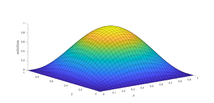
Figure 1: Exact solution $u_{\text{ex}}(x,t)=\sin(\pi x)\sin(\pi t)$.

In Figure 2, we show the error plot for the SU($\theta=1$) formulation on the same uniform meshes in space and time $\widehat{h}_{1}=\widehat{h}_{t}=:h$ and degrees $p=2,\ldots,5$. We can see that the method is not optimally convergent due to its leaks of consistency.

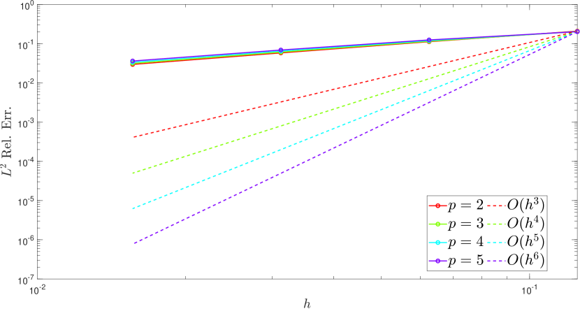
Figure 2: unsteady linear diffusion–reaction equation, SU($\theta=1$) relative error plots in $L^{2}$-norm, for $p=2,\ldots,5$.

The Figure 3 shows the error plot for the SU formulation on the same uniform meshes in space and time $\widehat{h}_{1}=\widehat{h}_{t}=:h$ and spline degrees $p=2,\ldots,5$. We can see the optimal convergence order of the method, due to the presence of the function $\theta(\boldsymbol{x},t)$ in (11) that deactivates the stabilization terms.

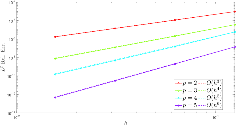
Figure 3: unsteady linear diffusion–reaction equation, SU relative error plots in $L^{2}$-norm, for $p=2,\ldots,5$.

5.2 Rogers-McCulloch model for cardiac electrophysiology

In this Section we want to analyse the numerical behaviour of the proposed stabilization method, in space–time Isogeometric Analysis framework, applied on Rogers-McCulloch model (8) on different spatial domain $\Omega$. In addition we set $C_{m}=1$, $D=10^{-4}$ (reasonable values, as proposed in [21]) and, following [23], $a=0.13$, $b=0.013$, $c_{1}=0.26$, $c_{2}=0.1$ and $d_{e}=1$. In particular, we consider a concentrated source term in space that acts over a short time interval when compared to the simulation time. The convergence tolerance in the fixed point iterations is set equal to $10^{-2}$.

5.2.1 First test: a rectangle

For the first test we consider a rectangular spatial domain $\Omega$. We consider uniform meshes along each parametric direction and we set $\widehat{h}_{1}=2^{-6}$, $\widehat{h}_{2}=2^{-3}$, $\widehat{h}_{t}=2^{-7}$ and $p=2$. So we solve the equation system on $(0,L_{1})\times(0,L_{2})\times(0,T)$ with $L_{1}=1.5$, $L_{2}=0.25$ and $T=300$ and the source term $f$ as follows:

$$f(x,y,t)=1/4\exp(-(5\cdot 10^{2}((y-0.5L_{2})^{2}+(x-1.6L_{1}t/T)^{2})))\ \chi_{[90,100]}(t),$$

where

$$\chi_{[90,100]}(t)=\left\{\begin{array}[]{llllll}1&\ \ \text{for}\ t\in[90,100],\\ 0&\ \ \text{otherwise}.\end{array}\right.$$

In Figures 4, 5 and 6 the numerical solutions of Galerkin, SU($\theta=1$) and SU methods are presented. We can see the function $\theta(x,y,t)$ that regulates the Spline Upwind activation in SU method in Figure 7. We observe the emergence of spurious oscillations in the case of the plain Galerkin method. On the other hand, when examining the numerical results of the stabilization methods, we can see that spurious oscillations are negligible.

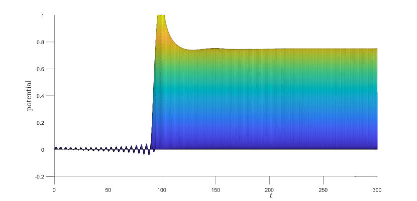
Figure 4: Two numerical solution views of the plain Galerkin method for the Rogers-McCulloch model ($\Omega$ is a rectangle), for $y=0.125$, with $\widehat{h}_{1}=2^{-6}$, $\widehat{h}_{2}=2^{-3}$, $\widehat{h}_{t}=2^{-7}$ and $p=2$.

Figure 5: Two numerical solution views of the SU($\theta=1$) method for the Rogers-McCulloch model ($\Omega$ is a rectangle), for $y=0.125$, with $\widehat{h}_{1}=2^{-6}$, $\widehat{h}_{2}=2^{-3}$, $\widehat{h}_{t}=2^{-7}$ and $p=2$.

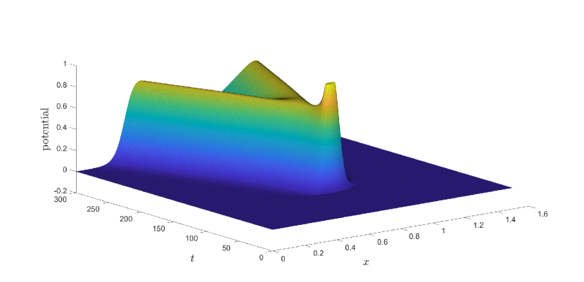
Figure 6: Two numerical solution views of the SU method for the Rogers-McCulloch model ($\Omega$ is a rectangle), for $y=0.125$, with $\widehat{h}_{1}=2^{-6}$, $\widehat{h}_{2}=2^{-3}$, $\widehat{h}_{t}=2^{-7}$ and $p=2$.

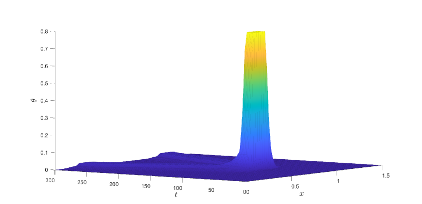
Figure 7: The function $\theta(x,y,t)$ ($\Omega$ is a rectangle), for $y=0.125$, with $\widehat{h}_{1}=2^{-6}$, $\widehat{h}_{2}=2^{-3}$, $\widehat{h}_{t}=2^{-7}$ and $p=2$.

Regarding the computational time of this first test, it is important to highlight that the time of the SU($\theta=1$) is approximately 1.5 times the calculation time of the plain Galerkin method while the time of the SU is approximately 5 times the calculation time of Galerkin method.

5.2.2 Second test: half annulus

For the second test we use half annulus as spatial domain $\Omega$ (Figure 8) and $(0,T)$ as time interval, with $T=300$, $\widehat{h}_{1}=2^{-6}$, $\widehat{h}_{2}=2^{-3}$, $\widehat{h}_{1}=2^{-7}$ and $p=2$. The source term $f$ is as follows:

$$f(x,y,t)=1/4\exp(-((y-1)^{2}+10^{3}(x-t/T)^{2}))\ \chi_{[90,100]}(t).$$

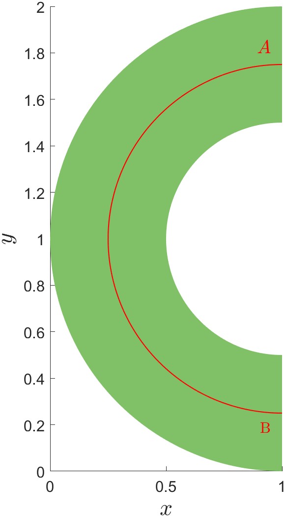
Figure 8: Half annulus with section line A–B depicted in red.

Figure 9 shows the Galerkin numerical solution for a fixed time $t=250$. In Figures 10, 11 and 12 the numerical solutions of Galerkin, SU($\theta=1$) and SU methods are showed, while the function $\theta(x,y,t)$ that regulates the Spline Upwind activation in SU method is presented in Figure 13. Also in this second test the plain Galerkin method presents spurious oscillation and these numerical instabilities are negligible in the SU($\theta=1$) and in SU methods.

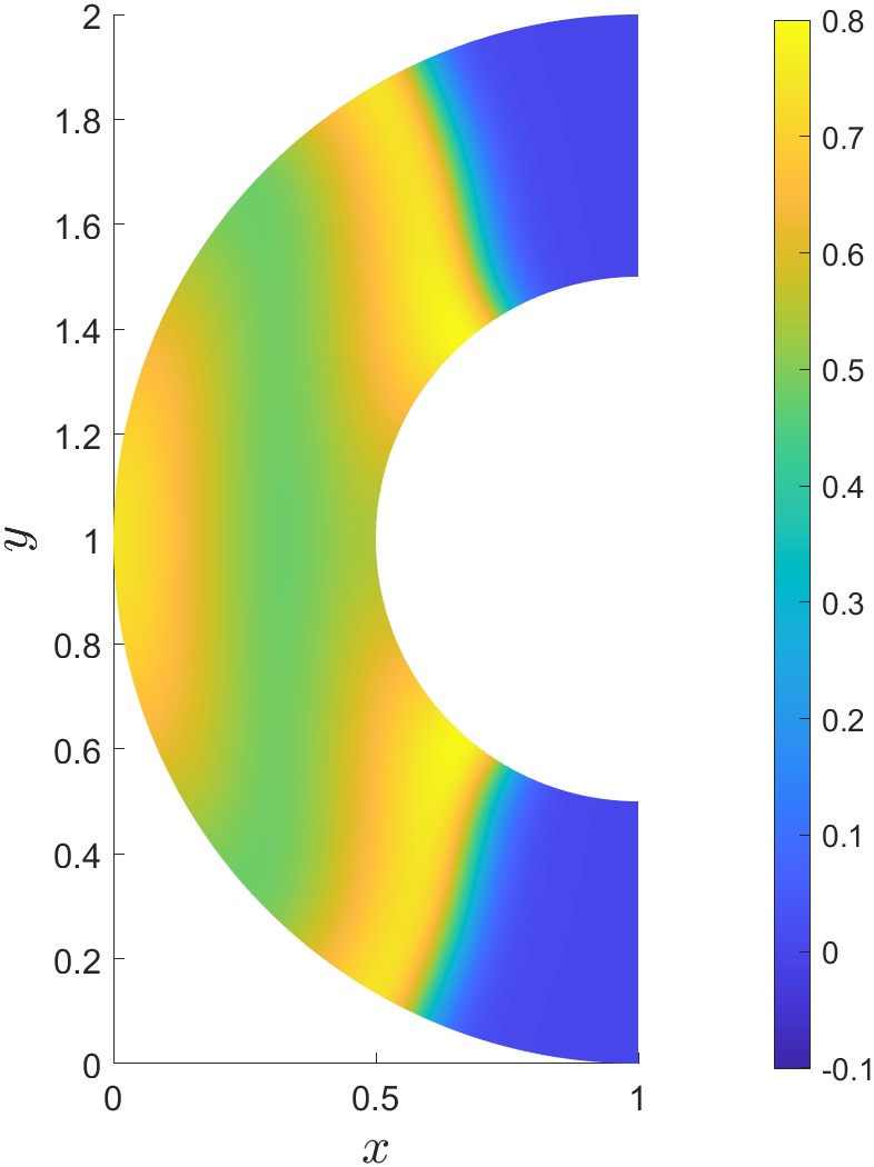
Figure 9: Numerical solution of the Galerkin method ($t=250$) for the Rogers-McCulloch model ($\Omega$ is half annulus) with $\widehat{h}_{1}=2^{-6}$, $\widehat{h}_{2}=2^{-3}$, $\widehat{h}_{1}=2^{-7}$ and $p=2$; the colors represent transmembrane potential.

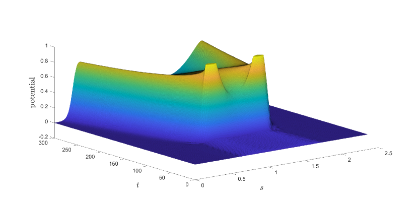
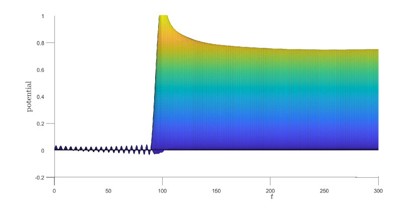
Figure 10: Two numerical solution views of the plain Galerkin method along the section line A–B for the Rogers-McCulloch model ($\Omega$ is half annulus) with $\widehat{h}_{1}=2^{-6}$, $\widehat{h}_{2}=2^{-3}$, $\widehat{h}_{1}=2^{-7}$ and $p=2$.

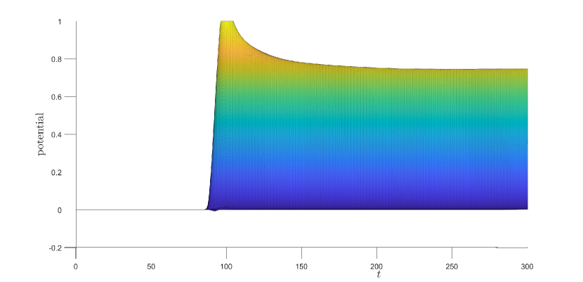
Figure 11: Two numerical solution views of the SU($\theta=1$) method along the section line A–B for the Rogers-McCulloch model ($\Omega$ is half annulus) with $\widehat{h}_{1}=2^{-6}$, $\widehat{h}_{2}=2^{-3}$, $\widehat{h}_{1}=2^{-7}$ and $p=2$.

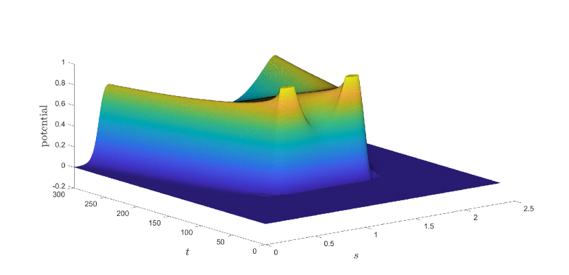
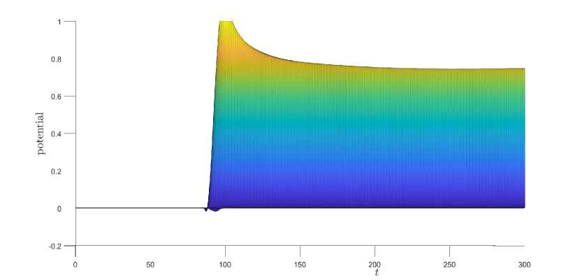
Figure 12: Two numerical solution views of the SU method along the section line A–B for the Rogers-McCulloch model ($\Omega$ is half annulus) with $\widehat{h}_{1}=2^{-6}$, $\widehat{h}_{2}=2^{-3}$, $\widehat{h}_{1}=2^{-7}$ and $p=2$.

Figure 13: The function $\theta(x,y,t)$ along the section line A–B for the Rogers-McCulloch model ($\Omega$ is half annulus) with $\widehat{h}_{1}=2^{-6}$, $\widehat{h}_{2}=2^{-3}$, $\widehat{h}_{1}=2^{-7}$ and $p=2$.

Regarding the computational time of this second test, we remark that the time of the SU($\theta=1$) is approximately 2.5 times the calculation time of the plain Galerkin method, while the time of the SU is approximately 10 times the calculation time of Galerkin method. These time increases are mainly due to the slower convergence in fixed point iterations. We can explain this fact taking in account that in SU($\theta=1$) the stabilization acts on all the domain and not only in the sharp layers, while in SU method we have a further non-linearity based on the residual.

6 Conclusions

The aim of the work is to propose a solver free of spurious oscillations for evolutionary problems related to cardiac electrophysiology. To do this we used a variant of the stabilization introduced in [17], which is based on the idea of respect the principle of causality, which is generally lost in space-time formulations.

Various numerical benchmarks highlight the optimal order of convergence for smooth solutions in unsteady linear diffusion–reaction case and an accurate and stable behaviour in the presence of sharp layers in the Rogers-McCulloch model. Furthermore, in order to complete the analysis of the method, we have quantified the computational time increase, going from plain Galerkin method to SU.

Finally we acknowledge the importance of efficient and fast solvers in the space–time framework: the higher dimensionality poses computational challenges if we want to investigate three dimensional spatial domains that generate 4D space–time domains. This issue is important for the the linear systems that need fast solvers with preconditioned iterative methods. We plan to explore the aspects on fast solvers in future works.

References

- [1] T. J. R. Hughes, J. A. Cottrell, Y. Bazilevs, Isogeometric analysis: CAD, finite elements, NURBS, exact geometry and mesh refinement, Computer Methods in Applied Mechanics and Engineering 194 (39) (2005) 4135–4195. doi:10.1016/j.cma.2004.10.008.
- [2] J. A. Evans, Y. Bazilevs, I. Babuška, T. J. R. Hughes, -widths, sup-infs, and optimality ratios for the -version of the isogeometic finite element method, Computer Methods in Applied Mechanics and Engineering 198 (2009) 1726–1741. doi:10.1016/j.cma.2009.01.021.
- [3] A. Bressan, E. Sande, Approximation in FEM, DG and IGA: a theoretical comparison, Numerische Mathematik 143 (4) (2019) 923–942. doi:10.1007/s00211-019-01063-5.
- [4] I. Fried, Finite-element analysis of time-dependent phenomena, AIAA Journal 7 (6) (1969) 1170–1173. doi:10.2514/3.5299.
- [5] J. T. Oden, A general theory of finite elements. II. Applications, International Journal for Numerical Methods in Engineering 1 (3) (1969) 247–259. doi:10.1002/nme.1620010304.
- [6] J. H. Argyris, D. W. Scharpf, Finite elements in time and space, Nuclear Engineering and Design 10 (4) (1969) 456–464. doi:10.1016/0029-5493(69)90081-8.
- [7] J. C. Bruch Jr., G. Zyvoloski, Transient two-dimensional heat conduction problems solved by the finite element method, International Journal for Numerical Methods in Engineering 8 (3) (1974) 481–494. doi:10.1002/nme.1620080304.
- [8] H. Nguyen, J. Reynen, A space-time least-square finite element scheme for advection-diffusion equations, Computer Methods in Applied Mechanics and Engineering 42 (3) (1984) 331–342. doi:10.1016/0045-7825(84)90012-4.
- [9] T. J. R. Hughes, G. M. H. Hulbert, Space-time finite element methods for elastodynamics: Formulations and error estimates, Computer Methods in Applied Mechanics and Engineering 66 (3) (1988) 339–363. doi:10.1016/0045-7825(88)90006-0.
- [10] C. Schwab, R. Stevenson, Space-time adaptive wavelet methods for parabolic evolution problems, Mathematics of Computation 78 (267) (2009) 1293–1318. doi:10.1090/S0025-5718-08-02205-9.
- [11] O. Steinbach, Space-Time Finite Element Methods for Parabolic Problems, Computational Methods in Applied Mathematics 15 (4) (2015) 551–566. doi:10.1515/cmam-2015-0026.
- [12] K. Takizawa, T. Tezduyar, Space-time computation techniques with continuous representation in time (ST-C), Computational Mechanics 53 (1) (2014) 91–99. doi:10.1007/s00466-013-0895-y.
- [13] U. Langer, S. E. Moore, M. Neumüller, Space-time isogeometric analysis of parabolic evolution problems, Computer Methods in Applied Mechanics and Engineering 306 (2016) 342 – 363. doi:10.1016/j.cma.2016.03.042.
- [14] C. Saadé, S. Lejeunes, D. Eyheramendy, R. Saad, Space-Time Isogeometric Analysis for linear and non-linear elastodynamics, Computers & Structures 254 (2021) 106594. doi:10.1016/j.compstruc.2021.106594.
- [15] M. Montardini, M. Negri, G. Sangalli, M. Tani, Space-time least-squares isogeometric method and efficient solver for parabolic problems, Mathematics of Computation 89 (323) (2020) 1193–1227. doi:10.1090/mcom/3471.
- [16] G. Loli, M. Montardini, G. Sangalli, M. Tani, An efficient solver for space-time isogeometric Galerkin methods for parabolic problems, Computers and Mathematics with Applications 80 (11) (2020) 2586–2603. doi:10.1016/j.camwa.2020.09.014.
- [17] G. Loli, G. Sangalli, P. Tesini, High-order spline upwind for space–time Isogeometric Analysis, Computer Methods in Applied Mechanics and Engineering 417 (11) (2023) 116408. doi:10.1016/j.cma.2023.116408.
- [18] A. N. Brooks, T. J. R. Hughes, Streamline upwind/Petrov-Galerkin formulations for convection dominated flows with particular emphasis on the incompressible Navier-Stokes equations, Computer Methods in Applied Mechanics and Engineering 32 (1) (1982) 199–259. doi:10.1016/0045-7825(82)90071-8.
- [19] P. Colli Franzone, L. F. Pavarino, S. Scacchi, Mathematical cardiac electrophysiology, Vol. 13, Springer, 2014.
- [20] A. Quarteroni, T. Lassila, S. Rossi, R. Ruiz-Baier, Integrated Heart—Coupling multiscale and multiphysics models for the simulation of the cardiac function, Computer Methods in Applied Mechanics and Engineering 314 (2017) 345–407, special Issue on Biological Systems Dedicated to William S. Klug. doi:10.1016/j.cma.2016.05.031.
- [21] A. S. Patelli, L. Dedè, T. Lassila, A. Bartezzaghi, A. Quarteroni, Isogeometric approximation of cardiac electrophysiology models on surfaces: An accuracy study with application to the human left atrium, Computer Methods in Applied Mechanics and Engineering 317 (2017) 248–273. doi:10.1016/j.cma.2016.12.022.
- [22] L. Pegolotti, L. Dedè, A. Quarteroni, Isogeometric Analysis of the electrophysiology in the human heart: Numerical simulation of the bidomain equations on the atria, Computer Methods in Applied Mechanics and Engineering 343 (2019) 52–73. doi:10.1016/j.cma.2018.08.032.
- [23] J. Rogers, A. McCulloch, A collocation-Galerkin finite element model of cardiac action potential propagation, IEEE Transactions on Biomedical Engineering 41 (8) (1994) 743–757. doi:10.1109/10.310090.
- [24] J. A. Cottrell, T. J. R. Hughes, Y. Bazilevs, Isogeometric analysis: toward integration of CAD and FEA, John Wiley & Sons, 2009.
- [25] L. B. da Veiga, A. Buffa, G. Sangalli, R. Vázquez, Mathematical analysis of variational isogeometric methods, Acta Numerica 23 (2014) 157–287. doi:10.1017/S096249291400004X.
- [26] A. Mantzaflaris, B. Jüttler, B. N. Khoromskij, U. Langer, Low rank tensor methods in Galerkin-based isogeometric analysis, Computer Methods in Applied Mechanics and Engineering 316 (2017) 1062–1085, special Issue on Isogeometric Analysis: Progress and Challenges. doi:https://doi.org/10.1016/j.cma.2016.11.013.
- [27] R. Vázquez, A new design for the implementation of isogeometric analysis in Octave and Matlab: GeoPDEs 3.0, Computers & Mathematics with Applications 72 (3) (2016) 523–554. doi:10.1016/j.camwa.2016.05.010.
- [28] Y. Wenjian, G. Yu, L. Yaohang, Efficient Randomized Algorithms for the Fixed-Precision Low-Rank Matrix Approximation, SIAM Journal on Matrix Analysis and Applications 39 (3) (2018) 1339–1359. doi:10.1137/17M1141977.