Spherical Frustum Sparse Convolution Network for LiDAR Point Cloud
Semantic Segmentation

Abstract

LiDAR point cloud semantic segmentation enables the robots to obtain fine-grained semantic information of the surrounding environment. Recently, many works project the point cloud onto the 2D image and adopt the 2D Convolutional Neural Networks (CNNs) or vision transformer for LiDAR point cloud semantic segmentation. However, since more than one point can be projected onto the same 2D position but only one point can be preserved, the previous 2D image-based segmentation methods suffer from inevitable quantized information loss. To avoid quantized information loss, in this paper, we propose a novel spherical frustum structure. The points projected onto the same 2D position are preserved in the spherical frustums. Moreover, we propose a memory-efficient hash-based representation of spherical frustums. Through the hash-based representation, we propose the Spherical Frustum sparse Convolution (SFC) and Frustum Fast Point Sampling (F2PS) to convolve and sample the points stored in spherical frustums respectively. Finally, we present the Spherical Frustum sparse Convolution Network (SFCNet) to adopt 2D CNNs for LiDAR point cloud semantic segmentation without quantized information loss. Extensive experiments on the SemanticKITTI and nuScenes datasets demonstrate that our SFCNet outperforms the 2D image-based semantic segmentation methods based on conventional spherical projection. The source code will be released later.

1 Introduction

Nowadays, 3D LiDAR point clouds are widely used sensor data in autonomous robot systems [4]. Semantic segmentation on the LiDAR point cloud enables the robot a fine-grained understanding of the surrounding environment.

Inspired by the achievements of deep learning in image semantic segmentation, researchers focus on searching for effective approaches to transfer the achievements to the field of point cloud semantic segmentation. Most of the previous works convert the raw point cloud to regular grids, like 2D images [30, 31, 21, 36, 10, 38, 18, 2, 27, 8, 3] and 3D voxels [9, 42, 37, 20], to exploit Convolutional Neural Networks (CNNs) and transformers in the field of point cloud semantic segmentation. The CNNs and transformer can easily process the regular grids and effectively segment the point cloud. However, due to the limited resolution, more than one point can be converted to the same grid, and only one point is preserved, which poses quantized information loss to the regular grid-based point cloud semantic segmentation methods. Some methods [21, 18] are proposed to compensate for the quantized information loss by restoring complete semantic predictions from partial predictions. However, quantized information loss still exists in the feature aggregation.

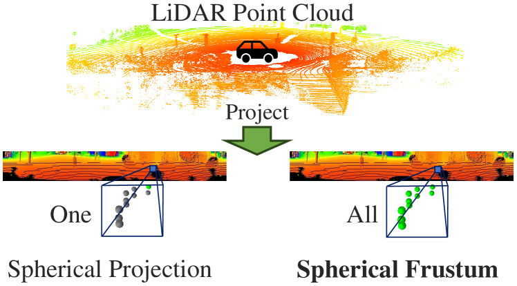
Figure 1: Difference Between Our Spherical Frustum and Conventional Spherical Projection. In the spherical projection, when multiple points are projected onto the same grid, only the nearest one green point is preserved while the redundant gray points are dropped. Compared to spherical projection, the spherical frustum structure does not drop the redundant points but preserves all green points projected onto the same 2D grid in the frustum. Therefore, spherical frustum can eliminate quantized information loss and preserve the complete geometric structure.

To exploit 2D CNNs in point cloud semantic segmentation without quantized information loss, in this paper, a novel spherical frustum structure is proposed. Fig. 1 shows the comparison between the conventional spherical projection [30] and spherical frustum. Spherical frustum stores all the points projected onto the same 2D grid. Therefore, spherical frustum can avoid the quantized information loss during the projection. However, without specific designs, the spherical frustum is an irregular structure and can not be processed by CNNs. Using dense grids to store the spherical frustums is an intuitive method to regularize the spherical frustum. However, since the point number of the spherical frustums is different, each point set is required to be padded to the maximal point number of the spherical frustums before being stored in the dense grid, which results in many redundant memory costs. Therefore, inspired by 3D sparse convolution [12], we propose the hash-based spherical frustum representation. The hash-based spherical frustum representation stores spherical frustums in a memory-efficient way. The neighbor relationship of spherical frustums and points is represented through the hash table, which enables the points to be simply stored in the original irregular point set. Specifically, in the hash-based representation, each point is uniquely identified by the hash key, which consists of the 2D coordinates of the corresponding spherical frustum and the point index in the spherical frustum point set. Thus, the points projected onto any specific 2D grids can be efficiently queried. Based on the hash-based representation, we propose the Spherical Frustum sparse Convolution (SFC) to exploit 2D CNNs on spherical frustums. SFC aggregates the point features in the nearby spherical frustums.

Moreover, previous 2D image-based segmentation methods downsample the projected point cloud based on stride-based 2D sampling, which is unable to uniformly sample the 3D point cloud. However, the stride-based 2D sampling uniformly samples the spherical frustums. Therefore, we propose a novel uniform point cloud sampling method, Frustum Farthest Point Sampling (F2PS). F2PS firstly samples spherical frustums by stride, and then uniformly samples the point set inside each sampled spherical frustum by Farthest Point Sampling (FPS) [26]. Since the computing complexity of sampling points in each spherical frustum is constant-level, F2PS is an efficient sampling algorithm with a linear computing complexity.

In summary, our contributions are:

• We propose a novel spherical frustum structure with a memory-efficient hash-based representation. Spherical frustum avoids quantized information loss of spherical projection and preserves complete geometric structure.

• We integrate spherical frustum structure into 2D sparse convolution, and propose a novel Spherical Frustum sparse Convolution Network (SFCNet) for LiDAR point cloud semantic segmentation.

• An efficient and uniform 3D point cloud sampling named frustum farthest point sampling is proposed based on the spherical frustum structure.

• SFCNet is evaluated on the SemanticKITTI [4] and nuScenes [6] datasets. The experiment results show that SFCNet outperforms previous 2D image-based methods.

2 Related Work

Point-Based Semantic Segmentation.   A group of works [26, 32, 29, 39, 15, 40, 33] learn to segment point cloud based on the raw unstructured point cloud. However, learning of raw point cloud requires the neighborhood query with high computing complexity to learn effective features from the local point cloud structure. Therefore, the efficiency of these point-based methods is limited.

3D Sparse Voxel-Based Semantic Segmentation.   Storing large-scale LiDAR point clouds in dense 3D voxels requires huge memory consumption. Therefore, Graham et al [12] proposes the 3D sparse voxel structure. Instead of dense grids, the hash table is adopted to represent the neighborhood relations of the 3D sparse grids. Based on the hash table, the convolved grids are recorded in the rule book. According to the rule book, the 3D sparse convolution is performed. Based on the sparse 3D voxel architecture, the methods of 3D sparse convolution and 3D attention mechanisms [9, 42, 37, 23, 19, 20] are proposed. In this paper, we get inspired by the 3D sparse voxel representation and exploit the hash table to represent the neighbor relationship of spherical frustums without redundant memory cost.

2D Image-Based Semantic Segmentation.   The research of image semantic segmentation [7, 16, 24, 28, 35] has gained great achievement. Thus, many works [30, 31, 21, 36, 10, 41, 2, 27, 8, 3, 38, 18] project the point cloud onto the 2D plane and utilize 2D neural networks to process the projected point cloud. Spherical projection is a widely used projection method first introduced by SqueezeSeg [30]. The subsequent works [30, 31, 21, 36, 41, 8, 3] effectively segment the point cloud with the image semantic segmentation architecture including 2D CNNs and vision transformers.

Due to the limited resolution, the 2D image-based segmentation methods suffer from quantized information loss. With quantized information loss, networks can only process the incomplete geometric structure and output partial semantic predictions, which results in the penalty of segmentation performance. The previous works only focus on restoring complete semantic predictions from the partial predictions of 2D neural networks. RangeNet++  [21] proposes a post-processing strategy to restore the complete predictions. The semantic predictions of dropped points are voted by the predictions of their K-Nearest Neighbors (KNN). In addition to KNN-based post-processing, KPRNet [18] directly reprojects incomplete predictions to the complete point cloud and adopts point-based network KPConv [29] to refine the predictions. However, few works explore the method of preserving the complete geometric structure during projection.

In this paper, we propose the spherical frustum which avoids the quantized information loss of spherical projection. Our spherical frustum structure can not only preserve the complete geometric structure but also output the complete semantic predictions without any post-processing or point-based network refinement.

3 SFCNet

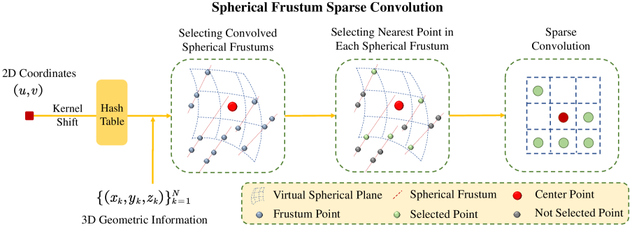
Figure 2: Pipeline of Spherical Frustum Sparse Convolution. The spherical frustums in the convolution kernel and the points in these spherical frustums are first selected through the hash table. Then, the nearest point in each spherical frustum is determined by the 3D geometric information. Finally, the sparse convolution is performed on the selected point features.

In this section, the spherical frustum and the hash-based representation will be first illustrated in Sec. 3.1. Then, we will introduce the spherical frustum sparse convolution and frustum farthest point sampling in Sec. 3.2 and 3.3 respectively. Finally, in Sec. 3.4, the architecture of the Spherical Frustum sparse Convolution Network (SFCNet) will be presented.

3.1 Spherical Frustum

Conventional Spherical Projection.  The LiDAR point cloud $\mathcal{P}$ is composed of $N$ points. The $k$-th point in $\mathcal{P}$ is represented by its 3D coordinates $\boldsymbol{x}_{k}=[x_{k},y_{k},z_{k}]^{T}$ and the input point features $\boldsymbol{f}_{k}\in\mathbb{R}^{C_{in}}$, where $C_{in}$ represents the channel dimension of the features. The conventional spherical projection [30] first calculates the 2D spherical coordinates of each point:

$$\left(\begin{matrix}u_{k}\\ v_{k}\end{matrix}\right)=\left(\begin{matrix}\frac{1}{2}[1-\arctan(y_{k},x_{k})\pi^{-1}]\cdot W\\ [1-(\arcsin(z_{k}/r_{k})+f_{down})\cdot f^{-1}]\cdot H\end{matrix}\right),$$ (1)

where $(H,W)$ is the height and width of the projected image. $r_{k}=\sqrt{x_{k}^{2}+y_{k}^{2}+z_{k}^{2}}$ is the range of the point. $f=f_{up}+f_{down}$ is the vertical field-of-view of the LiDAR sensor, where $f_{up}$ and $f_{down}$ are the up and down vertical field-of-views respectively. According to the computed 2D spherical coordinates, the point features $\{\boldsymbol{f}_{k}\}_{k=1}^{N}$ are projected onto the 2D dense image. If multiple points have the same 2D coordinates, the conventional spherical projection only projects the point closest to the origin and drops the other points, which results in the quantized information loss.

From Spherical Projection to Spherical Frustum.   Since dropping the redundant points projected onto the same 2D position results in quantized information loss, we propose the spherical frustum to preserve all the points projected onto the same 2D position. Specifically, we organize these points as a point set and assign each point with the unique index $m_{k}$ in the point set. In addition, the 3D coordinates of each point $\{(x_{k},y_{k},z_{k})\}_{k=1}^{N}$ are preserved as the 3D geometric information for the subsequent modules.

Hash-Based Spherical Frustum Representation.   The irregular spherical frustums can not be directly processed by the 2D CNNs. A natural idea to regularize the spherical frustums is putting them in dense grids. To store the point set of each spherical frustum in the dense grids, an extra grid dimension is required. The size of this dimension should be the maximal point number $M$ of each spherical frustum point set. However, since most of the spherical frustum point numbers are much less than $M$, many grids are empty. This phenomenon is similar to storing 3D sparse LiDAR point clouds in dense 3D voxels. Therefore, inspired by the 3D sparse convolution, we propose the hash-based spherical frustum representation to regularize the spherical frustum. In the hash table, the index $k$ of any point in the original point cloud can be queried using the key $(u_{k},v_{k},m_{k})$, which is the combination of the 2D spherical coordinates and the point index in the spherical frustum point set. Based on the hash-based representation, the spherical frustums are regularly stored in a memory-efficient way.

3.2 Spherical Frustum Sparse Convolution

Since multiple points are stored in a single spherical frustum, the conventional 2D convolution can not be directly performed on the spherical frustum structure. Therefore, we propose Spherical Frustum sparse Convolution (SFC). As shown in Fig. 2, SFC can be seen as the sparse convolution on the virtual spherical plane of the center point. The feature of each convolved 2D position on the virtual spherical plane is filled with the feature of the nearest points in the corresponding spherical frustum.

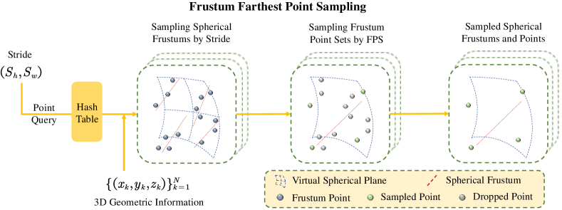
Figure 3: Pipeline of Frustum Farthest Point Sampling. According to the downsampling strides, the spherical frustums in each stride window are downsampled. Then, through the hash table, the points in each downsampled spherical frustum are queried. The queried points are sampled by Farthest Point Sampling (FPS) based on the 3D geometric information. Finally, the uniformly sampled spherical frustums and point cloud are simultaneously obtained.

Selecting Convolved Spherical Frustums.  Specifically, SFC first selects the convolved spherical frustums for each center point $p$. The 3D coordinates and the 2D spherical coordinates of the center point $p$ are $(x,y,z)$ and $(u,v)$ respectively. The conventional 2D convolution convolves the features of the grids in the convolution kernel. Similar to the conventional convolution, the spherical frustum of each 2D position in the convolution kernel is selected to perform the convolution. The coordinates of the 2D positions are $\{(u+\Delta u_{i},v+\Delta v_{i})\}_{i=1}^{K^{2}}$, where $K$ is the kernel size and $(\Delta u_{i},\Delta v_{i})$ are the shift inside the kernel. Then, the points inside each spherical frustum are queried through the hash table. Meanwhile, the features $\{\boldsymbol{f}_{j}\}_{j=1}^{M_{i}}$ of these points are obtained, where $M_{i}$ is the number of the points in the $i$-th spherical frustum. Notably, $M_{i}$ can be zero, which means that no points are projected onto the corresponding 2D position, and the spherical frustum is invalid. Like the 3D sparse convolution, the invalid spherical frustums are ignored in the subsequent convolution.

Selecting the Nearest Point in Each Spherical Frustum.  After identifying the points in the spherical frustums, the nearest point to the center point is selected. Based on the 3D geometric information, the 3D coordinates $\{(x_{j},y_{j},z_{j})\}_{j=1}^{M_{i}}$ of the frustum points are obtained for the nearest point selection. Inspired by the post-processing of RangeNet++ [21], we select the distance of range $r_{j}=\sqrt{x_{j}^{2}+y_{j}^{2}+z_{j}^{2}}$ rather than the Euclidean distance as the metric of the nearest point for efficient distance calculation. Therefore, the selected point index of each spherical frustum is $\arg\min_{j}\lvert r_{j}-r\rvert$, where $r$ is the range of the center point. According to the indexes, the convolved features $\{\boldsymbol{f}_{i}\}_{i=1}^{K^{\prime}}$ are obtained, where $K^{\prime}$ is the number of valid spherical frustums.

Sparse Convolution.  Finally, the sparse convolution is performed as:

$$\boldsymbol{f}^{\prime}=\sum_{i=1}^{K^{\prime}}W_{i}\boldsymbol{f}_{i},$$ (2)

where $W_{i}$ is the convolution weight of the $i$-th valid 2D position, and $\boldsymbol{f}^{\prime}$ is the aggregated feature.

Through the proposed spherical frustum sparse convolution, we realize effective regularization and 2D convolution-based feature aggregation for the unstructured point cloud.

3.3 Frustum Farthest Point Sampling

Sampling is a significant process of point cloud semantic segmentation. Through sampling, the network can aggregate the features of different scales and recognize objects of different sizes. Moreover, the sampling should uniformly sample the point cloud to avoid key information loss. The previous 2D image-based methods sample the projected point cloud using stride-based 2D sampling. This sampling ignores the 3D geometric structure of the point cloud. In contrast, as shown in Fig. 3, our Frustum Farthest Point Sampling (F2PS) only samples the spherical frustums by stride, while the spherical frustum point set is sampled by farthest point sampling.

Sampling Spherical Frustums by Stride.   Specifically, we split the 2D spherical plane into several non-overlapping windows of size $S_{h}\times S_{w}$, where $(S_{h},S_{w})$ are the strides. The spherical frustums in each window are merged as the downsampled spherical frustum. Meanwhile, the points inside the merged spherical frustums are queried through the hash table. Then, the queried points are merged as the point set $\{p_{l}\}_{l=1}^{L}$ in the downsampled spherical frustum, where $L$ is the point number in the downsampled spherical frustum.

Sampling Frustum Point Set by Farthest Point Sampling.   The Farthest Point Sampling (FPS) [26] is adopted to uniformly sample the point set in the spherical frustum. Since the point number of each spherical frustum is much smaller than the point number of the point cloud, performing FPS is not time-consuming. Specifically, the 3D coordinates of each point in $\{p_{l}\}_{l=1}^{L}$ are first acquired from the 3D geometric information for 3D distance calculation. Then, the $\lceil L/(S_{h}\times S_{w})\rceil$ points are iteratively sampled from the original point set. At each iteration, the distance of each non-sampled point towards the sampled point set is calculated. The point that has the maximal distance is added to the sampled set. Finally, the uniformly sampled spherical frustum point set is obtained.

F2PS integrates the stride-based spherical frustum sampling with the FPS-based frustum point set sampling. Thus, F2PS can sample the original point cloud uniformly. In addition, since performing FPS on the frustum point set costs $O(1)$ time, the computing complexity of F2PS is $O(N)$. Thus, F2PS is an efficient point cloud sampling algorithm.

3.4 Network Architecture

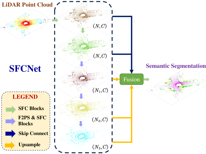
Figure 4: Overview of SFCNet Architecture. In SFCNet, the Spherical Frustum sparse Convolutional (SFC) blocks and Frustum Farthest Point Sampling (F2PS) are adopted to aggregate the point features of different scales. The point features of different scales are upsampled to the original scale and fused. Finally, SFC blocks decode the fused features and output the semantic segmentation.

Based on the Spherical Frustum sparse Convolution (SFC) and Frustum Farthest Point Sampling (F2PS), the Spherical Frustum sparse Convolution Network (SFCNet) is constructed, as shown in Fig. 4. Specifically, SFCNet first builds the hash-based spherical frustum representation for convolution and sampling in the subsequent modules. Then, the point features are extracted through the encoder of SFCNet. The encoder consists of the residual convolutional blocks from ResNet [13], where the convolutions are replaced by the proposed SFC. In addition, the point cloud is downsampled based on F2PS to extract the features of different scales. The extracted point features are $\mathcal{F}_{1}\in\mathbb{R}^{N\times C},\mathcal{F}_{2}\in\mathbb{R}^{N\times C},\mathcal{F}_{3}\in\mathbb{R}^{N_{1}\times C},\mathcal{F}_{4}\in\mathbb{R}^{N_{2}\times C}$, and $\mathcal{F}_{5}\in\mathbb{R}^{N_{3}\times C}$, where $N$, $N_{1}$, $N_{2}$, and $N_{3}$ are the point number of different layers respectively, and $C$ is the channel dimension of point features. Inspired by UperNet [34], we upsample and fuse the point features of the different scales in the decoder of SFCNet. Specifically, the upsampling is performed as:

$$\mathcal{F}^{\prime}_{i}=SFC(\mathcal{F}_{i}),$$ (3)

where $i\in\{3,4,5\}$, and $\mathcal{F}_{i}^{\prime}\in\mathbb{R}^{N\times C}$ is the $i$-th upsampled point features. $SFC$ is the spherical frustum sparse convolution, where the points in the original point cloud are treated as the center points. $\mathcal{F}_{i}$ is convolved point features. Then, the upsampled features $\mathcal{F}_{3}^{\prime},\mathcal{F}_{4}^{\prime}$, and $\mathcal{F}_{5}^{\prime}$ are fused with the skip-connected features $\mathcal{F}_{1}$ and $\mathcal{F}_{2}$ by concatenation. The fused features are fed into SFC blocks to decode the features. Finally, the prediction of semantic segmentation is outputted through a linear layer.

4 Experiments

In this section, we first introduce the datasets adopted in the experiments and the implementation details of the SFCNet. Then, the quantitative results of the two datasets and the qualitative results of the SemanticKITTI dataset are presented. Finally, the ablation studies, comparison with restoring-based methods, and comparison of sampling methods are conducted to validate the effectiveness of the proposed modules.

4.1 Datasets

We train and evaluate SFCNet on the SemanticKITTI [4] and nuScenes [6] datasets, which provide point-wise semantic labels for large-scale LiDAR point clouds.

SemanticKITTI [4] dataset contains $43551$ LiDAR point cloud scans captured by the $64$-line Velodyne-HDLE64 LiDAR. Each scan contains nearly $120K$ points. These scans are split into $22$ sequences. According to the official setting, we split sequences 00-07 and 09-10 as the training set, sequence 08 as the validation set, and sequences 11-21 as the test set. Moreover, SemanticKITTI provides the point-wise semantic annotations of $19$ classes for the LiDAR semantic segmentation task.

NuScenes [6] dataset consists of $34149$ LiDAR point cloud scans collected in $1000$ autonomous driving scenes using the $32$-line Velodyne HDL-32E LiDAR. Each scan contains nearly $40K$ points. We adopt the official setting to split the scans of the nuScenes dataset into the training and validation sets. In addition, in nuScenes dataset, $16$-class point-wise semantic annotations are provided for the LiDAR semantic segmentation task.

On both datasets, the performance of LiDAR point cloud semantic segmentation is evaluated by mean Intersection-over-Union (mIoU) [11].

Table 1: Quantative results of semantic segmentation on the SemanticKITTI [4] test set. The bold results are the best in each column while the blue results are the second best.

Approach	mIoU (%)	car	bicycle	motorcycle	truck	other-vehicle	person	bicyclist	motorcyclist	road	parking	sidewalk	other-ground	building	fence	vegetation	trunk	terrain	pole	traffic-sign
3D Voxel Based
Cylinder3D [42]	67.8	97.1	67.6	64.0	59.0	58.6	73.9	67.9	36.0	91.4	65.1	75.5	32.3	91.0	66.5	85.4	71.8	68.5	62.6	65.6
2D Image Based
RangeNet++ [21]	52.2	91.4	25.7	34.4	25.7	23.0	38.3	38.8	4.8	91.8	65.0	75.2	27.8	87.4	58.6	80.5	55.1	64.6	47.9	55.9
PolarNet [38]	54.3	93.8	40.3	30.1	22.9	28.5	43.2	40.2	5.6	90.8	61.7	74.4	21.7	90.0	61.3	84.0	65.5	67.8	51.8	57.5
SqueezeSegV3 [36]	55.9	92.5	38.7	36.5	29.6	33.0	45.6	46.2	20.1	91.7	63.4	74.8	26.4	89.0	59.4	82.0	58.7	65.4	49.6	58.9
SalsaNext [10]	59.5	91.9	48.3	38.6	38.9	31.9	60.2	59.0	19.4	91.7	63.7	75.8	29.1	90.2	64.2	81.8	63.6	66.5	54.3	62.1
KPRNet [18]	63.1	95.5	54.1	47.9	23.6	42.6	65.9	65.0	16.5	93.2	73.9	80.6	30.2	91.7	68.4	85.7	69.8	71.2	58.7	64.1
Lite-HDSeg [27]	63.8	92.3	40.0	55.4	37.7	39.6	59.2	71.6	54.1	93.0	68.2	78.3	29.3	91.5	65.0	78.2	65.8	65.1	59.5	67.7
RangeViT [3]	64.0	95.4	55.8	43.5	29.8	42.1	63.9	58.2	38.1	93.1	70.2	80.0	32.5	92.0	69.0	85.3	70.6	71.2	60.8	64.7
CENet [8]	64.7	91.9	58.6	50.3	40.6	42.3	68.9	65.9	43.5	90.3	60.9	75.1	31.5	91.0	66.2	84.5	69.7	70.0	61.5	67.6
Sphercial Frustum Based
SFCNet (Ours)	65.0	95.1	64.2	63.2	23.5	45.6	78.3	73.1	26.4	87.9	65.6	71.9	29.1	91.1	64.5	83.7	72.6	69.6	62.6	67.2

Table 2: Quantative results of semantic segmentation on the nuScenes [6] validation set. The bold results are the best in each column while the blue results are the second best.

Approach	mIoU (%)	barrier	bicycle	bus	car	construction	motorcycle	pedestrian	traffic-cone	trailer	truck	driveable	other flat	sidewalk	terrain	manmade	vegetation
3D Voxel Based
Cylinder3D [42]	76.1	76.4	40.3	91.3	93.8	51.3	78.0	78.9	64.9	62.1	84.4	96.8	71.6	76.4	75.4	90.5	87.4
2D Image Based
RangeNet++ [21]	65.5	66.0	21.3	77.2	80.9	30.2	66.8	69.6	52.1	54.2	72.3	94.1	66.6	63.5	70.1	83.1	79.8
PolarNet [38]	71.0	74.7	28.2	85.3	90.9	35.1	77.5	71.3	58.8	57.4	76.1	96.5	71.1	74.7	74.0	87.3	85.7
SalsaNext [10]	72.2	74.8	34.1	85.9	88.4	42.2	72.4	72.2	63.1	61.3	76.5	96.0	70.8	71.2	71.5	86.7	84.4
RangeViT [3]	75.2	75.5	40.7	88.3	90.1	49.3	79.3	77.2	66.3	65.2	80.0	96.4	71.4	73.8	73.8	89.9	87.2
Spherical Frustum Based
SFCNet (Ours)	75.9	76.7	40.4	89.5	91.3	46.7	82.0	78.1	65.8	69.4	80.6	96.6	71.6	74.5	74.9	89.0	87.5

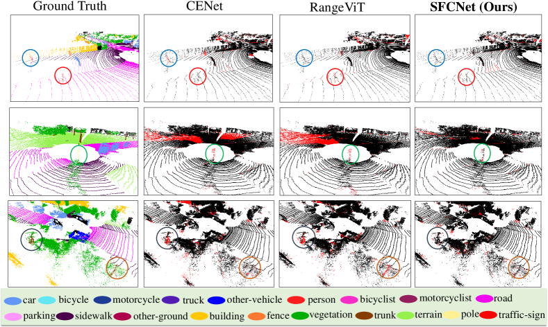
Figure 5: Qualitive results on SemanticKITTI [4] validation set. The first column presents the ground truths, while the following three columns show the error maps of the predictions of the three methods. Specifically, the reference from point color to the semantic class in the ground truths is shown at the bottom. In addition, the false-segmented points are marked as red in the error maps. Moreover, we use circles with the same color to point out the same objects in the ground truth and the three error maps.

4.2 Implementation Details

We implement SFCNet by PyTorch [25] framework. For spherical frustum, we set the height and width in the calculation of spherical coordinates as $H=64,W=1800$ for SemanticKITTI, and $H=32,W=1024$ for nuScenes. The channel dimensions $C$ of the extracted point features for SemanticKITTI and nuScenes datasets are set as $128$ and $256$ respectively. The strides $(S_{h},S_{w})$ in the three downsampling layers are all set as $(2,2)$. We use multi-layer weighted cross-entropy loss and Lovász-Softmax loss [5] to optimize the framework. In addition, during training, we use Adam [17] optimizer with the initial learning rate $0.001$. The learning rate is delayed by $5\%$ in every epoch. We utilize the data augmentations including random rotation, flipping, translation, and scaling for the training on the two datasets.

4.3 Quantative Results

We compare our spherical frustum-based 2D segmentation method, SFCNet, to State-of-The-Art (SoTA) 2D image-based segmentation methods and the representative 3D voxel-based segmentation method Cylinder3D [42] on the SemanticKITTI and nuScenes datasets.

Table 3: Results of ablation studies on the SemanticKITTI validation set.

ID	Baseline	SFC	F2PS	mIoU (%)
1	✓			56.2
2	✓	✓		60.5
3	✓	✓	✓	62.9

As shown in Tables 1 and 2, SFCNet outperforms the previous SoTA 2D convolution-based segmentation methods CENet [8] and SalsaNext [10] on the SemanticKITTI and nuScenes respectively. In addition, SFCNet also has better performance than the vision transformer-based segmentation method RangeViT [3] on both two datasets. Compared to the 3D voxel-based method, SFCNet realizes a smaller performance gap between the 2D convolution-based methods and the 3D convolution-based method Cylinder3D [42], since the spherical frustum structure avoids the quantized information loss. As for the per-class IoU comparison, SFCNet has better IoU than the other 2D image-based methods on the small 3D objects, including the motorcycle, person (which is pedestrian in nuScenes), bicyclist, trunk, and pole. SFCNet even performs better than the 3D voxel-based method on the person, bicyclist, trunk, and pole classes. The performance improvement on these small objects results from the elimination of quantized information loss. Without quantized information loss, the complete geometric structure of the small 3D objects can be preserved, which enables more accurate segmentation.

4.4 Qualitative Results

Fig. 5 presents the qualitative comparison between our SFCNet and the 2D image-based segmentation methods CENet [8] and RangeViT [3]. The comparison shows that the predictions of SFCNet have the minimal segmentation error among the three methods. Moreover, the circled objects in the three rows of Fig. 5 demonstrate the accurate segmentation of SFCNet to the persons, poles, and trunks respectively. This result further indicates our better segmentation performance of 3D small objects by eliminating the quantized information loss.

4.5 Ablation Study

In this section, we conduct the ablation study on the SemanticKITTI dataset to validate the effectiveness of the proposed modules. We adopt the baseline network using the conventional spherical projection and stride-based sampling. The results of ablation studies are shown in Table 3.

Spherical Frustum Sparse Convolution (SFC).   First, we replace spherical projection in the baseline with spherical frustum and adopt spherical frustum sparse convolution for feature aggregation. After replacement, the mIoU increases $4.3\%$, which indicates that spherical frustum structure can avoid the quantized information loss, and thus prevent segmentation error from incomplete predictions.

Frustum Farthest Point Sampling (F2PS).   After replacing the stride-based 2D sampling with the Frustum Farthest Point Sampling (F2PS), the mIoU increases $2.4\%$. F2PS uniformly samples the point cloud and preserves the key information. Thus, the performance of semantic segmentation has been improved.

4.6 Comparision with Restoring-Based Methods

Based on the same baseline network in Sec. 4.5, we compare our SFCNet with the methods that compensate for the quantized information loss by restoring complete predictions from partial predictions, including the KNN-based post-processing [21] and KPConv refinement [18]. Table 4 shows that SFCNet has $3.2\%$ mIoU improvement to the KNN-based post-processing and $3.3\%$ mIoU improvement to KPConv refinement. Compared to the restoring-based methods, SFCNet preserves the complete geometric structure for the feature aggregation rather than compensating for the information loss by post-processing or refinement, which results in higher performance of semantic segmentation.

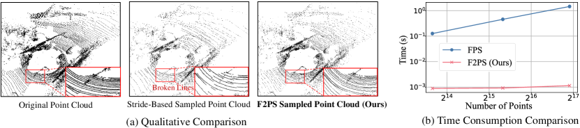
Figure 6: In this figure, (a) presents the qualitative comparison between stride-based 2D sampling and our Frustum Farthest Point Sampling (F2PS). The red boxes show the zoomed view of the point clouds in the close areas. (b) illustrates the time consumption comparison between Farthest Point Sampling (FPS) and our F2PS.

Table 4: The performance comparison between the restoring-based methods and SFCNet on the SemanticKITTI validation set.

Method	mIoU (%)
KNN-based Post-processing [21]	59.7
KPConv Refinement [18]	59.6
SFCNet (Ours)	62.9

4.7 Comparison of Sampling Methods

We further validate the effectiveness and efficiency of F2PS by the qualitative comparison with stride-based 2D sampling and the comparison of time consumption with Farthest Point Sampling (FPS).

Qualitive Comparison.  As shown in Fig. 6(a), Stride-Based 2D Sampling (SBS) only samples the point cloud based on 2D stride. The visualization shows that the stride-based sampled point cloud is relatively rough. Due to the lack of 3D geometric information, SBS fails to sample the 3D point cloud uniformly. Thus, the loss of geometric structure in the sampled point cloud is obvious, such as many broken lines on the ground. Our F2PS takes into account the 3D geometric information based on the FPS in the spherical frustum, which enables F2PS to sample the 3D point cloud uniformly and preserve the significant 3D geometric structure during the sampling.

Time Consumption Comparison.   As shown in Fig. 6(b), with the increment of sampled point number, the cost time of our F2PS increases slowly, while the cost time of FPS increases dramatically. This result shows performing FPS on the frustum point sets is efficient and does not increase the computing burden.

5 Conclusion

In this paper, we present the Spherical Frustum sparse Convolutional Network (SFCNet), a 2D convolution-based LiDAR point cloud segmentation method without quantized information loss. The quantized information loss is eliminated through the novel spherical frustum structure, which preserves all the points projected onto the same 2D position. Moreover, the novel spherical frustum sparse convolution and frustum farthest point sampling are proposed for effective convolution and sampling of the points stored in the spherical frustums. Experiment results on SemanticKITTI and nuScenes datasets show the better semantic segmentation performance of SFCNet compared to the previous 2D image-based semantic segmentation methods, especially on small objects. The results show the great potential of SFCNet for safe autonomous driving perception due to the accurate segmentation of small targets. The future work will focus on applying our spherical frustum structure to more tasks, like point cloud registration and scene flow estimation.

Figure 7: The Detailed Architecture of SFCNet. (a) presents the detailed pipeline of SFCNet. In addition, (b), (c), and (d) show the detailed module structures of the SFC layer, SFC block, and downsampling SFC block respectively, where SFC means spherical frustum sparse convolution, and F2PS means the frustum farthest point sampling.

Table 5: The Detailed Hyperparameters of the Components and Modules in SFCNet. Component shows the names of components in SFCNet. Module Type shows the types of basic modules used in the components. Kernel Size shows the convolution kernel size of Spherical Frustum sparse Convolutions (SFCs) used in the modules. In the column of Stride, $[1,1]$ strides mean the SFC treats all the points as the center points, while $[2,2]$ strides show the strides used in Frustum Farthest Point Sampling (F2PS). The column of Upsampling Rate shows the upsampling rate used in the upsampling SFCs. Number of Modules shows the number of composed modules used in corresponding components. Width shows the output channel dimensions of the modules. In addition, in the column of Width, $C$ means the channel dimensions of the extracted point features, which is $128$ for the SemanticKITTI dataset and $256$ for the nuScenes dataset. $n$ means the number of semantic classes, which is $19$ for the SemanticKITTI dataset and $16$ for the nuScenes dataset.

Component	Module Type	Kernel Size	Stride	Upsampling Rate	Number of Modules	Width
Context Block	SFC Layer	[3,3]	[1,1]	—	3	[C/2,C,C]
Extraction Layer 1	SFC Block	[3,3]	[1,1]	—	3	[C,C,C]
	Downsampling SFC Block	[3,3]	[2,2]	—	1	[C]
Extraction Layer 2	SFC Block	[3,3]	[1,1]	—	3	[C,C,C]
	Downsampling SFC Block	[3,3]	[2,2]	—	1	[C]
Extraction Layer 3	SFC Block	[3,3]	[1,1]	—	5	[C,C,C,C,C]
	Downsampling SFC Block	[3,3]	[2,2]	—	1	[C]
Extraction Layer 4	SFC Block	[3,3]	[1,1]	—	2	[C,C]
	Upsampling SFC for Extraction Layer 2	[3,3]	[1,1]	[2,2]	1	[C]
	Upsampling SFC for Extraction Layer 3	[7,7]	[1,1]	[4,4]	1	[C]
Upsampling	Upsampling SFC for Extraction Layer 4	[15,15]	[1,1]	[8,8]	1	[C]
	SFC Layer	[3,3]	[1,1]	—	2	[2$\cdot$C,C]
Head Layer	Linear	—	—	—	1	[n]

Appendix

In the appendix, we first introduce the detailed architecture of the Spherical Frustum sparse Convolution Network (SFCNet) in Sec. A. Then, the additional implementation details of SFCNet are presented in Sec. B. Next, the efficiency analysis of SFCNet is illustrated in Sec. C. Finally, more visualization of the semantic segmentation results on the SemanticKITTI [4] and nuScenes [6] datasets are presented in Sec. D.

Appendix A Detailed Architecture

Fig. 7 shows the detailed architecture of SFCNet. In SFCNet, the spherical frustum structure of the input point cloud is first constructed. Then, the encoder, which consists of the context block and extraction layers 1 to 4, is adopted for the point feature extraction. Next, in the decoder, the point features extracted in extraction layers 2 to 4 are upsampled by the upsampling Spherical Frustum sparse Convolution (SFC). The upsampled features are fused with the features extracted in the context block and in the extraction layer 1 to gain the multi-scale fused features. The fused features are fed into the head layer to decode the point features into the semantic predictions.

In addition, Fig. 7 also shows the three basic modules in SFCNet, including the SFC layer, SFC block, and downsampling SFC block. Moreover, we present the detailed hyperparameters of SFCNet in Table 5.

Basic Modules of SFCNet.   Specifically, the SFC layer is composed of the SFC, batch normalization, and the activation function. Inspired by [8], we use Hardswish [14] as the activation function. The formula of Hardswish is:

$$Hardswish(x)=\begin{cases}0&if\ x\leq-3\\ x&if\ x\geq 3\\ x\cdot(x+3)/6&otherwise\end{cases}.$$ (4)

The SFC block consists of two SFC layers. In addition, the residual connection [13] is adopted in the SFC block to overcome network degradation.

The downsampling SFC block combines the downsampling of Frustum Farthest Point Sampling (F2PS) and the feature aggregation of the SFC block. Notably, in the downsampling SFC block, the first SFC treats the sampled points as the center points and the features of the point cloud before sampling as the aggregated features.

Moreover, after the downsampling, the 2D coordinates of each spherical frustum are divided by the stride to gain the 2D coordinates on the downsampled 2D spherical plane. Meanwhile, each point is assigned a new point index in the downsampled spherical frustum point set according to the sampled order in F2PS.

Components in the Encoder of SFCNet.   In the encoder, the context block consists of three SFC layers to extract the initial point features from the original point cloud. The subsequent four extraction layers are composed of $3,3,5$, and $2$ SFC blocks respectively. In addition, a downsampling SFC block with $(2,2)$ strides is adopted in the last three layers to downsample the point cloud into different scales. Thus, the multi-scale point features are extracted.

Components in the Decoder of SFCNet.   We implement the upsampling SFC in the decoder of SFCNet according to the deconvolution [22] used in the 2D convolutional neural networks. In the upsampling SFC, we first multiply the 2D coordinates of the spherical frustums in the corresponding layer by the upsampling rate to obtain the 2D coordinates on the original spherical plane. Then, each point in the raw point cloud is treated as the center point in SFC. The spherical frustums fall in the convolution kernel are convolved. As shown in Table 5, we set the appropriate kernel size according to the upsampling rate for each upsampling SFC.

After the upsampling, the point features from different extraction layers are of the same size. Thus, we can concatenate the point features for fusion. In the head layer, two SFC layers and a linear layer are adopted for the decoding of the fused features.

Appendix B Additional Implementation Details

Data Normalization.   For the $k$-th point in the LiDAR point cloud $\mathcal{P}$, the combination of the 3D coordinates $\boldsymbol{x}_{k}=[x_{k},y_{k},z_{k}]^{T}$, the range $r_{k}=\sqrt{x_{k}^{2}+y_{k}^{2}+z_{k}^{2}}$, and the intensity is treated as the input point feature $\boldsymbol{f}_{k}$. Because of the different units of the different data categories, the input features should be normalized.

Specifically, for the SemanticKITTI [4] dataset, like RangeNet++ [21], we minus the features by the mean and divide the features by the standard deviation to obtain the normalized features. The mean and standard deviation are obtained from the statistics of each input data category on the SemanticKITTI dataset, which are presented in Table 6.

For the nuScenes [6] dataset, like Cylinder3D [42], a batch normalization layer is applied on the input point features to record the mean and standard deviation of the nuScenes dataset during training. During inferencing, the recorded mean and standard deviation are used to normalize the input point features.

Table 6: The statistics of each input data category on SemanticKITTI dataset.

Statistics	$x$	$y$	$z$	$range$	$intensity$
Mean	10.88	0.23	-1.04	12.12	0.21
Standard Deviation	11.47	6.91	0.86	12.32	0.16

Spherical Frustum Construction.   We construct the spherical frustum structure by assigning each point with the 2D spherical coordinates $(u_{k},v_{k})$ and the point index $m_{k}$ in the spherical frustum point set, where $k$ is the index of the point in the original point cloud. The 2D spherical coordinates can be calculated through Eq. 1. Thus, the key process is to assign the point index $m_{k}$ for each point based on the 2D spherical coordinates.

We implement this by sorting the 2D coordinates $(u_{k},v_{k})$ of the points. The points with smaller $u_{k}$ and $v_{k}$ are ranked ahead of the points with larger $u_{k}$ and $v_{k}$. Thus, the points with the same 2D coordinates are neighbors in the sorted point cloud. For each point, we count the number of points that have the same 2D coordinates and appear ahead or behind the point in the sorted point cloud separately. The number of the points appearing ahead is treated as the point index $m_{k}$ of each point.

In addition, we assign each point an indicator $\xi_{k}\in\{0,1\}$ according to the number of the points appearing behind. The point with zero point appearing behind is assigned a zero indicator. Otherwise, the point is assigned with an indicator equal to one. The indicator indicates the end of the frustum point set and is used for the subsequent spherical frustum point set visiting.

The sorting and the point number counting are implemented through the Graphics Processing Unit (GPU)-based parallel computing using Compute Unified Device Architecture (CUDA). Thus, the construction is efficient in practice.

Hash-Based Spherical Frustum Representation.   After the construction of the spherical frustum structure, we build the hash-based spherical frustum representation. Specifically, we construct the key-value pairs between the key $(u_{k},v_{k},m_{k})$ and the value $k$. The key-value pairs are inserted into a hash table, which represents the neighbor relationship of spherical frustums and points.

In practice, we adopt an efficient GPU-based hash table [1]. The GPU-based hash table requires both key and value to be an integer. The value $k$ satisfies the integer requirement. However, the key $(u_{k},v_{k},m_{k})$ in the hash-based spherical frustum representation is not an integer.

To adopt the GPU-based hash table for efficient processing, $(u_{k},v_{k},m_{k})$ is transferred to an integer as $v_{k}\cdot(W\cdot M)+u_{k}\cdot M+m_{k}$, where $W$ is the width of the spherical projection, $M$ is the maximal point number of the spherical frustum point sets. Through this process, any point represented by the coordinates $(u_{k},v_{k},m_{k})$ can be efficiently queried through the GPU-based hash table.

Spherical Frustum Point Set Visiting.   Both the SFC and F2PS require visiting all the points in any spherical frustums. Thus, we propose the spherical frustum point set visiting algorithm. The visiting obtains all the points in the given spherical frustum, whose 2D coordinates are $(u,v)$, by sequentially querying the points in the hash table.

Specifically, we first query the first point in the spherical frustum using the key $(u,v,0)$. If the key $(u,v,0)$ is not in the hash table, the spherical frustum on $(u,v)$ is invalid. Otherwise, the first point in the spherical frustum can be queried through the hash table.

Then, the points in the spherical frustum are sequentially visited. We first initialize the point index $m=0$ in the spherical frustum. At each step, the point index $m$ increases by one. Through the hash table, the point with $m$-th index in the spherical frustum is queried using the key $(u,v,m)$. Meanwhile, the indicator $\xi$ of this point is obtained. $\xi$ indicates whether $(u,v,m+1)$ refers to a valid point. Thus, the visiting ends when the indicator of the current point is zero.

Detailed Implementation of Frustum Farthest Point Sampling.   In F2PS, we first sample the spherical frustums by stride. Then, we sample the points in each sampled spherical frustum by Farthest Point Sampling (FPS) [26]. As mentioned in Sec. 3.3, FPS is an iterative algorithm. The detailed process of the $j$-th iteration can be expressed by the following formula:

$$S_{j}=S_{j-1}\cup\{\arg\max_{p\in P_{s}\backslash S_{j-1}}\min_{s\in S_{j-1}}dist(p,s)\},$$ (5)

where $P_{s}$ is the spherical frustum point set to be sampled, $S_{j}$ and $S_{j-1}$ are the sampled point sets in $j$-th and $(j-1)$-th iterations respectively. Notably, $S_{0}$ contains the point randomly sampled from $P_{s}$. In addition, $dist(p,s)$ is the distance between point $p$ and point $s$ in 3D space. The iteration starts at $j=1$, and ends when the size of $S_{k}$ equals the number of sampling points.

Moreover, since the distances between the points in $S_{j-2}$ and the points in $P_{s}\backslash S_{j-1}$ have been calculated before the $j$-th iteration, we just need to calculate the distance between each $p$ in $P_{s}\backslash S_{j-1}$ and the point sampled in $(j-1)$-th iteration for the calculation of $\min_{s\in S_{j-1}}dist(p,s)$, which is the minimal distance from point $p$ to the point set $S_{j-1}$. Thus, the computing complexity of FPS for $P_{s}$ of size $n$ is $O(n^{2})$. Since the point number of each spherical frustum is $O(1)$, the computing complexity of FPS for the spherical frustum is also $O(1)$, which ensures the efficiency of F2PS.

Loss Function.   We use multi-layer weighted cross-entropy loss and Lovász-Softmax loss [5] to help the network learn the semantic information from different scales. To get the semantic predictions of extraction layers 1 to 4, we apply a linear layer to decode the extracted point features of each extraction layer into the semantic predictions.

Specifically, for extraction layer 1, the linear layer is applied on the extracted point features $\mathcal{F}_{1}$ to gain the prediction $\tilde{L}_{1}$. For the other extraction layers, the linear layer is applied on the upsampled point features $\mathcal{F}^{\prime}_{2}$, $\mathcal{F}^{\prime}_{3}$, and $\mathcal{F}^{\prime}_{4}$ to obtain the predictions $\tilde{L}_{2}$, $\tilde{L}_{3}$, and $\tilde{L}_{4}$ respectively.

Based on the predictions of each layer and the final predictions of SFCNet $\tilde{L}_{0}$, the loss function is calculated as:

$$\mathcal{L}=\sum_{i=0}^{4}\mathcal{L}_{wce}(\tilde{L}_{i},L)+\mathcal{L}_{Lov}(\tilde{L}_{i},L),$$ (6)

where $\mathcal{L}_{wce}$ is the weighted cross-entropy loss, $\mathcal{L}_{Lov}$ is the Lovász-Softmax loss, and $L$ is the ground truth. In addition, the weights of weighted cross-entropy loss are calculated as $w_{c}=(f_{c}+\epsilon)^{-1}$, where $c$ is the semantic class, $f_{c}$ is the frequency of class $c$ in the dataset, and $\epsilon$ is a small positive value to avoid zero division.

Table 7: Efficiency and Performance Comparison. We conduct the efficiency and performance comparison among the baseline, RangeViT [3], and the proposed SFCNet on the SemanticKITTI [4] validation set. For efficiency, the inference time of a single LiDAR scan, the processed point number, and the Normalized Time (NT), which is the inference time per thousand points, are evaluated. In addition, the performance is evaluated by the mean Intersection-over-Union (mIoU).

Approach	Time (ms)/Points $\downarrow$	NT (ms/$K$) $\downarrow$	mIoU (%) $\uparrow$
Baseline	46.4/$\sim 90K$	0.52	56.2
RangeViT [3]	104.8/$\sim 120K$	0.87	60.8
SFCNet (Ours)	59.7/$\bf{\sim 120K}$	0.49	62.9

Appendix C Efficiency Analysis

We evaluate the efficiency of the baseline model, RangeViT [3], and the proposed SFCNet on a single Geforce RTX 4090Ti GPU.

We adopt the same baseline model used for the ablation study in Sec. 4.5. For RangeViT, we adopt the official code and pre-trained model for efficiency and performance evaluation. Notably, in the inference, RangeViT splits the projected LiDAR image, inputs each image slice into the network to gain the predictions, and merges the predictions to gain the prediction of the entire projected LiDAR image. Thus, the inference time of RangeViT includes the time of all the processes. In addition, since RangeViT adopts the KPConv refinement [18], which restores the complete predictions from the partial predictions, we use the point number of the entire point cloud as the processed point number.

The results are presented in Table 7. In addition, the performance of semantic segmentation is also illustrated in Table 7. The results show that SFCNet costs $59.7$ ms for inference, which shows SFCNet can reach the real-time processing for the large-scale LiDAR point cloud. In addition, our SFCNet also has the highest efficiency evaluated by normalized time ($0.49$ ms) and the best performance ($62.9\ \%$) among the baseline model, RangeViT [3], and our SFCNet.

Appendix D More Visualization

To better demonstrate the effectiveness of SFCNet for LiDAR point cloud semantic segmentation, we conducted more visualization on the SemanticKITTI [4] and nuScenes [6] datasets. The results are shown in Fig. 8, 9, and 10.

Qualitive Comparison on NuScenes Validation Set.   The results of qualitative comparison between our SFCNet and RangeViT [3] is shown in Fig. 8. On the nuScenes validation set, SFCNet can also have fewer segmentation errors than RangeViT as the results in the SemanticKITTI dataset. Moreover, the better segmentation accuracy of the 3D small objects, like pedestrians and motorcycles, can also be observed on the nuScenes validation set. The results once more demonstrate semantic segmentation improvement of SFCNet due to the overcoming of quantized information loss.

More Qualitative Comparison on SemanticKITTI Test Set.   The ground truths on the SemanticKITTI test set are not available. Thus, we search for the corresponding RGB image and project the semantic predictions on the image to compare the semantic segmentation accuracy between the state-of-the-art 2D image-based method CENet [8] and our SFCNet on the SemanticKITTI test set. As shown in Fig. 9, compared to CENet [8], SFCNet can more accurately segment the LiDAR point cloud in various challenging scenes on the SemanticKITTI test set.

Specifically, in the crowded street of Fig. 9(a), SFCNet can successfully segment the boxed person, who is distant and close to the wall of the building, while CENet confuses the person with the building wall. In the village road of Fig. 9(b), SFCNet recognizes the thin pole in distance and fully segments the pole, while CENet predicts the bottom of the pole as the building class. In the wild road of Fig. 9(c), SFCNet recognizes the thin trunk inside the vegetation while CENet wrongly predicts the trunk as the fetch. These results further validate the better segmentation performance of SFCNet to 3D small objects.

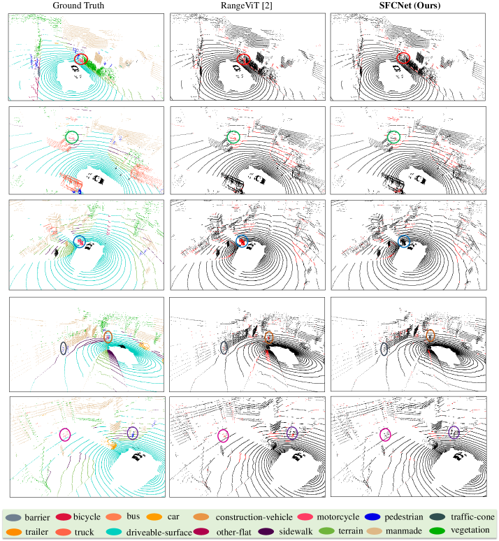
Figure 8: Qualitative Comparison on NuScene [6] Validation Set. In this figure, we conducted the qualitative comparison between RangeViT [3] and our SFCNet of semantic segmentation on the nuScenes validation set. The first column presents the ground truths, while the following two columns show the error maps of the predictions of RangeViT [3] and our SFCNet respectively. In addition, the reference from point color to the semantic class in the ground truths is shown at the bottom. Moreover, the false-segmented points are marked as red in the error maps. Furthermore, we use circles with the same color to point out the same objects in the ground truth and the two error maps.

More Qualitative Comparison on NuScenes Validation Set.   As the visualization on the SemanticKITTI test set, we provide the additional qualitative comparison between our SFCNet and RangeViT [3] on the nuScene validation set with the projected predictions illustrated in Fig. 10. The results further demonstrate the better semantic segmentation of SFCNet for the challenging street scenes on the nuScenes validation set compared to RangeViT.

Specifically, in the first scene, the close motorcycle can be correctly segmented by SFCNet, while RangeViT recognizes the motorcycle as a car, which shows that SFCNet can help the autonomous car correctly recognize the type of close obstacles, and enable the car to make appropriate decisions.

In the second scene, the distant pedestrians on the other side of the crossing can also be correctly segmented by SFCNet due to the elimination of quantized information loss. In contrast, RangeViT wrongly predicts the pedestrians as traffic cones.

In the third scene, since the boxed pedestrian is close to the manmade, RangeViT confuses it with the manmade and does not segment the pedestrian, while our SFCNet can clearly recognize the boundary and successfully segments the pedestrian.

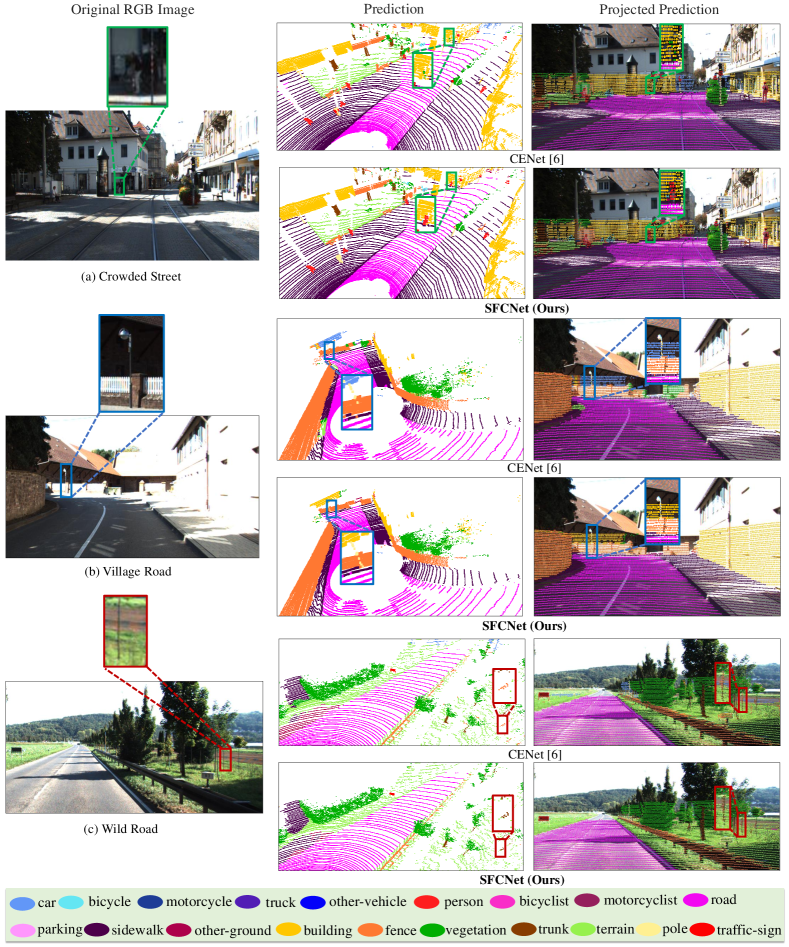
Figure 9: More Qualitative Comparison on Semantic Segmentation on SemanticKITTI [4] Test Set. We show the qualitative comparison between our SFCNet and the state-of-the-art 2D image-based method CENet [8] on the SemanticKITTI [4] dataset. The visualized challenging autonomous driving scenes include the street, the village, and the wild. The predictions projected on the corresponding RGB images are also illustrated. In addition, we use the same color boxes to point out the same objects in the point clouds and images for each scene. Meanwhile, we provide the zoomed-in view of some boxed objects for clear visualization. Moreover, the reference from point color to the semantic class in the predictions is shown at the bottom of the figure.

Figure 10: More Qualitative Comparison of Semantic Segmentation on NuScenes [6] Validation Set. We show more comparisons between our SFCNet and the state-of-the-art 2D image-based method RangeViT [3] on the nuScenes dataset. The predictions projected on the corresponding RGB images are also illustrated. In addition, we use the same color boxes to point out the same objects in the point clouds and images for each scene. Meanwhile, we provide the zoomed-in view of some boxed objects for clear visualization. Moreover, the reference from point color to the semantic class in the predictions and ground truths is shown at the bottom of the figure.

References

- Alcantara et al. [2012] Dan A Alcantara, Vasily Volkov, Shubhabrata Sengupta, Michael Mitzenmacher, John D Owens, and Nina Amenta. Building an efficient hash table on the gpu. In GPU Computing Gems Jade Edition, pages 39–53. Elsevier, 2012.
- Alnaggar et al. [2021] Yara Ali Alnaggar, Mohamed Afifi, Karim Amer, and Mohamed ElHelw. Multi projection fusion for real-time semantic segmentation of 3d lidar point clouds. In Proceedings of the IEEE/CVF Winter Conference on Applications of Computer Vision, pages 1800–1809, 2021.
- Ando et al. [2023] Angelika Ando, Spyros Gidaris, Andrei Bursuc, Gilles Puy, Alexandre Boulch, and Renaud Marlet. Rangevit: Towards vision transformers for 3d semantic segmentation in autonomous driving. Proceedings of the IEEE conference on computer vision and pattern recognition, 2023.
- Behley et al. [2019] Jens Behley, Martin Garbade, Andres Milioto, Jan Quenzel, Sven Behnke, Cyrill Stachniss, and Jurgen Gall. Semantickitti: A dataset for semantic scene understanding of lidar sequences. In Proceedings of the IEEE/CVF International Conference on Computer Vision, pages 9297–9307, 2019.
- Berman et al. [2018] Maxim Berman, Amal Rannen Triki, and Matthew B Blaschko. The lovász-softmax loss: A tractable surrogate for the optimization of the intersection-over-union measure in neural networks. In Proceedings of the IEEE conference on computer vision and pattern recognition, pages 4413–4421, 2018.
- Caesar et al. [2020] Holger Caesar, Varun Bankiti, Alex H Lang, Sourabh Vora, Venice Erin Liong, Qiang Xu, Anush Krishnan, Yu Pan, Giancarlo Baldan, and Oscar Beijbom. nuscenes: A multimodal dataset for autonomous driving. In Proceedings of the IEEE/CVF conference on computer vision and pattern recognition, pages 11621–11631, 2020.
- Chen et al. [2017] Liang-Chieh Chen, George Papandreou, Iasonas Kokkinos, Kevin Murphy, and Alan L Yuille. Deeplab: Semantic image segmentation with deep convolutional nets, atrous convolution, and fully connected crfs. IEEE transactions on pattern analysis and machine intelligence, 40(4):834–848, 2017.
- Cheng et al. [2022] Hui-Xian Cheng, Xian-Feng Han, and Guo-Qiang Xiao. Cenet: Toward concise and efficient lidar semantic segmentation for autonomous driving. In 2022 IEEE International Conference on Multimedia and Expo (ICME), pages 01–06. IEEE, 2022.
- Cheng et al. [2021] Ran Cheng, Ryan Razani, Ehsan Taghavi, Enxu Li, and Bingbing Liu. 2-s3net: Attentive feature fusion with adaptive feature selection for sparse semantic segmentation network. In Proceedings of the IEEE/CVF conference on computer vision and pattern recognition, pages 12547–12556, 2021.
- Cortinhal et al. [2020] Tiago Cortinhal, George Tzelepis, and Eren Erdal Aksoy. Salsanext: Fast, uncertainty-aware semantic segmentation of lidar point clouds. In Advances in Visual Computing: 15th International Symposium, ISVC 2020, San Diego, CA, USA, October 5–7, 2020, Proceedings, Part II 15, pages 207–222. Springer, 2020.
- Everingham et al. [2015] Mark Everingham, SM Ali Eslami, Luc Van Gool, Christopher KI Williams, John Winn, and Andrew Zisserman. The pascal visual object classes challenge: A retrospective. International journal of computer vision, 111:98–136, 2015.
- Graham et al. [2018] Benjamin Graham, Martin Engelcke, and Laurens Van Der Maaten. 3d semantic segmentation with submanifold sparse convolutional networks. In Proceedings of the IEEE conference on computer vision and pattern recognition, pages 9224–9232, 2018.
- He et al. [2016] Kaiming He, Xiangyu Zhang, Shaoqing Ren, and Jian Sun. Deep residual learning for image recognition. In Proceedings of the IEEE conference on computer vision and pattern recognition, pages 770–778, 2016.
- Howard et al. [2019] Andrew Howard, Mark Sandler, Grace Chu, Liang-Chieh Chen, Bo Chen, Mingxing Tan, Weijun Wang, Yukun Zhu, Ruoming Pang, Vijay Vasudevan, et al. Searching for mobilenetv3. In Proceedings of the IEEE/CVF international conference on computer vision, pages 1314–1324, 2019.
- Hu et al. [2021] Qingyong Hu, Bo Yang, Linhai Xie, Stefano Rosa, Yulan Guo, Zhihua Wang, Niki Trigoni, and Andrew Markham. Learning semantic segmentation of large-scale point clouds with random sampling. IEEE Transactions on Pattern Analysis and Machine Intelligence, 2021.
- Iandola et al. [2016] Forrest N Iandola, Song Han, Matthew W Moskewicz, Khalid Ashraf, William J Dally, and Kurt Keutzer. Squeezenet: Alexnet-level accuracy with 50x fewer parameters and 0.5 mb model size. arXiv preprint arXiv:1602.07360, 2016.
- Kingma and Ba [2014] Diederik P Kingma and Jimmy Ba. Adam: A method for stochastic optimization. arXiv preprint arXiv:1412.6980, 2014.
- Kochanov et al. [2020] Deyvid Kochanov, Fatemeh Karimi Nejadasl, and Olaf Booij. Kprnet: Improving projection-based lidar semantic segmentation. arXiv preprint arXiv:2007.12668, 2020.
- Lai et al. [2022] Xin Lai, Jianhui Liu, Li Jiang, Liwei Wang, Hengshuang Zhao, Shu Liu, Xiaojuan Qi, and Jiaya Jia. Stratified transformer for 3d point cloud segmentation. In Proceedings of the IEEE/CVF Conference on Computer Vision and Pattern Recognition, pages 8500–8509, 2022.
- Lai et al. [2023] Xin Lai, Yukang Chen, Fanbin Lu, Jianhui Liu, and Jiaya Jia. Spherical transformer for lidar-based 3d recognition. In Proceedings of the IEEE/CVF Conference on Computer Vision and Pattern Recognition, 2023.
- Milioto et al. [2019] Andres Milioto, Ignacio Vizzo, Jens Behley, and Cyrill Stachniss. RangeNet ++: Fast and Accurate LiDAR Semantic Segmentation. In 2019 IEEE/RSJ International Conference on Intelligent Robots and Systems (IROS), pages 4213–4220. IEEE, 2019.
- Noh et al. [2015] Hyeonwoo Noh, Seunghoon Hong, and Bohyung Han. Learning deconvolution network for semantic segmentation. In Proceedings of the IEEE international conference on computer vision, pages 1520–1528, 2015.
- Park et al. [2022] Chunghyun Park, Yoonwoo Jeong, Minsu Cho, and Jaesik Park. Fast point transformer. In Proceedings of the IEEE/CVF Conference on Computer Vision and Pattern Recognition, pages 16949–16958, 2022.
- Paszke et al. [2016] Adam Paszke, Abhishek Chaurasia, Sangpil Kim, and Eugenio Culurciello. Enet: A deep neural network architecture for real-time semantic segmentation. arXiv preprint arXiv:1606.02147, 2016.
- Paszke et al. [2019] Adam Paszke, Sam Gross, Francisco Massa, Adam Lerer, James Bradbury, Gregory Chanan, Trevor Killeen, Zeming Lin, Natalia Gimelshein, Luca Antiga, et al. Pytorch: An imperative style, high-performance deep learning library. Advances in neural information processing systems, 32, 2019.
- Qi et al. [2017] Charles Ruizhongtai Qi, Li Yi, Hao Su, and Leonidas J Guibas. Pointnet++: Deep hierarchical feature learning on point sets in a metric space. Advances in neural information processing systems, 30, 2017.
- Razani et al. [2021] Ryan Razani, Ran Cheng, Ehsan Taghavi, and Liu Bingbing. Lite-hdseg: Lidar semantic segmentation using lite harmonic dense convolutions. In 2021 IEEE International Conference on Robotics and Automation (ICRA), pages 9550–9556. IEEE, 2021.
- Redmon and Farhadi [2018] Joseph Redmon and Ali Farhadi. Yolov3: An incremental improvement. arXiv preprint arXiv:1804.02767, 2018.
- Thomas et al. [2019] Hugues Thomas, Charles R Qi, Jean-Emmanuel Deschaud, Beatriz Marcotegui, François Goulette, and Leonidas J Guibas. Kpconv: Flexible and deformable convolution for point clouds. In Proceedings of the IEEE/CVF international conference on computer vision, pages 6411–6420, 2019.
- Wu et al. [2018] Bichen Wu, Alvin Wan, Xiangyu Yue, and Kurt Keutzer. Squeezeseg: Convolutional neural nets with recurrent crf for real-time road-object segmentation from 3d lidar point cloud. In 2018 IEEE International Conference on Robotics and Automation (ICRA), pages 1887–1893. IEEE, 2018.
- Wu et al. [2019a] Bichen Wu, Xuanyu Zhou, Sicheng Zhao, Xiangyu Yue, and Kurt Keutzer. Squeezesegv2: Improved model structure and unsupervised domain adaptation for road-object segmentation from a lidar point cloud. In 2019 International Conference on Robotics and Automation (ICRA), pages 4376–4382. IEEE, 2019a.
- Wu et al. [2019b] Wenxuan Wu, Zhongang Qi, and Li Fuxin. Pointconv: Deep convolutional networks on 3d point clouds. In Proceedings of the IEEE/CVF Conference on computer vision and pattern recognition, pages 9621–9630, 2019b.
- Wu et al. [2023] Wenxuan Wu, Li Fuxin, and Qi Shan. Pointconvformer: Revenge of the point-based convolution. In Proceedings of the IEEE/CVF Conference on Computer Vision and Pattern Recognition, pages 21802–21813, 2023.
- Xiao et al. [2018] Tete Xiao, Yingcheng Liu, Bolei Zhou, Yuning Jiang, and Jian Sun. Unified perceptual parsing for scene understanding. In Proceedings of the European conference on computer vision (ECCV), pages 418–434, 2018.
- Xie et al. [2021] Enze Xie, Wenhai Wang, Zhiding Yu, Anima Anandkumar, Jose M Alvarez, and Ping Luo. Segformer: Simple and efficient design for semantic segmentation with transformers. Advances in Neural Information Processing Systems, 34:12077–12090, 2021.
- Xu et al. [2020] Chenfeng Xu, Bichen Wu, Zining Wang, Wei Zhan, Peter Vajda, Kurt Keutzer, and Masayoshi Tomizuka. Squeezesegv3: Spatially-adaptive convolution for efficient point-cloud segmentation. In European Conference on Computer Vision, pages 1–19. Springer, 2020.
- Ye et al. [2021] Maosheng Ye, Shuangjie Xu, Tongyi Cao, and Qifeng Chen. Drinet: A dual-representation iterative learning network for point cloud segmentation. In Proceedings of the IEEE/CVF international conference on computer vision, pages 7447–7456, 2021.
- Zhang et al. [2020] Yang Zhang, Zixiang Zhou, Philip David, Xiangyu Yue, Zerong Xi, Boqing Gong, and Hassan Foroosh. Polarnet: An improved grid representation for online lidar point clouds semantic segmentation. In Proceedings of the IEEE/CVF Conference on Computer Vision and Pattern Recognition, pages 9601–9610, 2020.
- Zhao et al. [2019] Hengshuang Zhao, Li Jiang, Chi-Wing Fu, and Jiaya Jia. Pointweb: Enhancing local neighborhood features for point cloud processing. In Proceedings of the IEEE/CVF conference on computer vision and pattern recognition, pages 5565–5573, 2019.
- Zhao et al. [2021a] Hengshuang Zhao, Li Jiang, Jiaya Jia, Philip HS Torr, and Vladlen Koltun. Point transformer. In Proceedings of the IEEE/CVF international conference on computer vision, pages 16259–16268, 2021a.
- Zhao et al. [2021b] Yiming Zhao, Lin Bai, and Xinming Huang. Fidnet: Lidar point cloud semantic segmentation with fully interpolation decoding. In 2021 IEEE/RSJ International Conference on Intelligent Robots and Systems (IROS), pages 4453–4458. IEEE, 2021b.
- Zhu et al. [2021] Xinge Zhu, Hui Zhou, Tai Wang, Fangzhou Hong, Yuexin Ma, Wei Li, Hongsheng Li, and Dahua Lin. Cylindrical and asymmetrical 3d convolution networks for lidar segmentation. In Proceedings of the IEEE/CVF conference on computer vision and pattern recognition, pages 9939–9948, 2021.