Boundary sensitive Lindbladians and relaxation dynamics
Abstract
It is well known that non-Hermitian systems can be extremely sensitive to boundary conditions owing to non-Hermitian skin effect (NHSE). Analogously, we investigate two boundary-sensitive symmetric Lindbladians: one carries current in the steady state, and the other does not. The numerical results indicate significant change of the Liouvillian spectrum, eigenmodes and relaxation time for both Lindbladians when the boundary conditions are altered. This phenomenon is found to be triggered by the Liouvillian skin effect (LSE), specifically the localization of eigenmodes, which stems from the NHSE of the non-Hermitian effective Hamiltonian. In addition, these two Lindbladians manifest different LSE, ultimately resulting in distinct relaxation behaviors.
I Introduction
Open quantum systems have attracted growing interest due to the rapid advancements in quantum technology, which enable the engineering of specific environments and the realization of diverse non-equilibrium phenomena [1, 2, 3, 4, 5, 6, 7, 8, 9]. Moreover, given the inevitable coupling between the system and the environment in practical applications, it is both essential and practical to explore physical processes encompassing system-environment interactions. Under Markovian approximation, it is widely acknowledged that the Lindblad master equation effectively describes the evolution of the system[10]. One pivotal quantity that characterizes this evolution is the relaxation time , serving as a significant intrinsic timescale. Another closely related quantity is Liouvillian gap , which is defined as the smallest modulus of the real part of nonzero eigenvalues of the Lindbladian. Conventionally, for open quantum systems governed by the Markovian Lindblad master equation, the relaxation time is approximately inversely proportional to the Liouvillian gap of the system. Therefore, extensive prior research has focused on investigating the scaling relationship between the Liouvillian gap and system size [11, 12, 13]. However, recent studies have uncovered the discrepancy between the inverse of the Liouvillian gap and the relaxation time [14, 15, 16, 17]. This anomalous relaxation behavior is attributed to superexponentially large expansion coefficients of Liouvillian eigenmodes.
On another front, recent works have uncovered numerous novel phenomena of non-Hermitian Hamiltonian, one of which is the extreme sensitivity of the boundary conditions, which originates from NHSE [18, 19, 20, 21, 22, 23, 24, 25, 26, 27, 28, 29, 30, 31, 32, 33, 34, 35, 36]. There are two marked signals for NHSE: one is accumulation of extensive eigenstates near the edge, and another is dramatic change of energy spectrum when switching boundary conditions. Evidently, NHSE will induce rich nontrivial dynamical effects, such as unconventional reflection, entanglement suppression, etc [37, 38, 39, 40, 41, 42, 43, 44]. However, the non-Hermitian Hamiltonian suffers from post-selection problem [45], which renders it exponentially hard to implement in experiments. So it is natural to ask how to design a post-selection free open quantum model hosting skin effect and how skin effect will shape the Liouvillian spectrum, eigenmodes (including steady state) and the relaxation dynamics?
The first question is answered inspired by recent progress on measurement-induced phase transition (MIPT) [46, 47, 48, 49, 50, 51, 52, 53, 54], which similarly encounters the post-selection issue. An interesting attempt to overcome the problem is to apply corrective unitary operations, as long as the unexpected measurement outcome appears. In doing so, the system can be steered towards a particular target state [55, 56, 57, 58, 59]. By choosing appropriate continuous measurement and feedback operators, recent studies successfully attain Liouvillian skin effect (LSE) in the steady state. The numerical findings corroborate that the skin effect effectively immobilizes a substantial portion of particles, thereby significantly suppressing the growth of entanglement and ultimately preventing the occurrence of MIPT[60, 61]. It is worthwhile to mention other mechanisms such as interactions [62] and asymmetric jump operators can also induce LSE[15, 63].
In this paper, we will address the second question. In order to clearly show the rich and nontrivial role of LSE, we investigate two Lindbladians, one with feedback and the other without, under both periodic boundary conditions (PBCs) and open boundary conditions (OBCs). The first Lindbladian holds a current-carrying steady state, whereas the second Lindbladian hosts a no-current steady state. It is reasonable to anticipate these two Lindbladian will manifest distinct relaxation behaviors. Our paper indeed demonstrates that LSE will greatly alters the Lindbladians’ eigenvalues and eigenmodes. Consequently, the relaxation behaviors are also fundamentally changed. Furthermore, the Lindbladians studied in this paper can be well understood by perturbation theory, which unveils the close connections between the NHSE of non-Hermitian effective Hamiltonian and the LSE of the whole Lindbladian. For clarity, we adopt NHSE to denote skin effect for the eigenstates of the non-Hermitian Hamiltonian, while LSE represents skin effect for the eigenmodes of the Lindbladians, despite both of them sharing the same mathematical origin.
The rest of the paper is organized as follows: in Sec. II, we introduce two Lindbladians and their corresponding measurement protocols. Next, Sec. III provides a brief overview of some basic knowledge of Lindbladians. Subsequently, we proceed to present our research findings. Firstly, in Sec. IV, the Lindbladian with feedback is investigated. Specifically, in Sec. IV.1.1, we acquire Liouvillian spectra for different monitoring rate under OBCs and PBCs. Secondly, the Sec. IV.1.2 shows that the eigenmodes including steady state under OBCs exhibit LSE, while the eigenmodes under PBCs are extended. Thirdly, in Sec. IV.1.3, utilizing exact diagonalization, we obtain scaling relation between the Liouvillian gap and system size for OBCs and PBCs. We find the relaxation time scales as under OBCs, and under PBCs. The former displays discrepancy between the inverse of the Liouvillian gap and the relaxation time, which approximately follows , while the latter obeys . Interestingly, cutoff phenomenon exists under OBCs. In Sec. IV.2, we consider the half-filled many-body case in brief, in which the LSE and cutoff phenomenon survive. The scaling relations between and remain valid. In Sec. V, the Lindbladian without feedback is investigated. Although the steady state and eigenmodes around steady state are free from LSE, the majority of eigenmodes still display LSE. Hence, the Liouvillian spectrum, Liouvillian gap and relaxation time are also dramatically altered when changing boundary conditions. Interestingly, we observe that the relaxation time is smaller than the inverse of Liouvillian gap under PBCs, i.e. , while for the OBCs, the relaxation time still satisfies the usual rule . Appendix. A presents a perturbation analysis of Liouvillian spectrum and eigenmodes. Exact solutions of the nontrivial steady state under PBCs are also available. Lastly, in Appendix. B, some additional numerical results are provided to support our conclusions. The main results of the paper are summarized in table. 1.
| steady | the majority | relaxation | relaxation | cutoff | Liouvillian gap vs | |
|---|---|---|---|---|---|---|
| state | of eigenmodes | time vs | time vs | phenomena | relaxation time | |
| Feedback, PBCs | extended | monotonic | not exist | |||
| Feedback, OBCs | LSE | LSE | non-monotonic | exist | ||
| No-feedback, PBCs | for ; for | extended | , | monotonic | not exist | |
| No-feedback, OBCs | LSE | non-monotonic | not exist |
II Lindbladians and Measurement Protocols
The measurement protocols to achieve the Lindbladians we studied have been illustrated in detail before [60, 61]. Here, we will briefly introduce them for completeness. We consider a one-dimensional (1D) free fermion model, subject to continuous measurement and unitary feedback. The Hamiltonian is given by
| (1) |
where () denotes annihilation (creation) operator of the spinless fermion at site and represents the hopping strength. We set throughout the work. The measurement operators act on two neighboring sites and can be expressed as , in which . To achieve nontrivial steady state exhibiting LSE, additional subsequent unitary feedback operator should be applied after measurement. The unitary feedback operator is expressed as . Thus, for the Lindbladian with feedback, the corresponding Lindblad operator is
| (2) |
Furthermore, we also consider the Lindbladian without feedback. In this scenario, the Lindblad operator simplifies to the measurement operator alone, represented as . It is noted that is invariant with unitary feedback. In addition, both Lindbladians are number-conserving, or symmetric.
For continuously monitored systems, it is widely acknowledged that the system’s evolution is described by the Lindblad master equation within the framework of the Markovian approximation[51]. The master equation is as follows:
| (3) |
where is referred to as Lindbladian or Liouvillian superoperator and denotes Lindblad operator mentioned previously. Furthermore, represents the monitoring rate, namely the frequency for the environment observing the system. It should be noted that the Lindblad operators are quadratic in the single-particle sector. Moreover, we highlight that both Lindbladians (with and without feedback) share the same effective non-Hermitian Hamiltonian , which can be expressed as
| (4) | ||||
Neglecting overall dissipation, corresponds to the Hatano-Nelson model[64], renowned for its manifestation of NHSE under OBCs. The eigenstates display exponential localization characterized by , in which and . Conversely, under PBCs, owing to , the non-Hermitian effective Hamiltonian shares common eigenstates with free fermion Hamiltonian . As a result, the eigenvalues are , in which , and . In the Appendix. A, perturbation theory explicitly demonstrates that the sensitivity of the Lindbladian is inherited from the sensitivity of non-Hermitian effective Hamiltonian .
In this paper, we investigate two Lindbladians, corresponding to feedback case and no-feedback case, respectively. Both of them are boundary-sensitive, but it is noteworthy that there is an essential difference between the cases with and without feedback. Specifically, under PBCs, for the former, the system carries current in the steady state, while the latter adheres to detailed balance condition, resulting in a vanishing current[61]. Therefore, it is reasonable to anticipate distinct relaxation dynamics between the Lindbladians with and without feedback.
Before delving into our findings, we emphasize the difference of the present work with previous works, which concentrate on the entanglement dynamics by utilizing the quantum jump method to approximately simulate evolution of the system, in terms of the stochastic Schrödinger equation[60, 61]. In contrast, our work primarily focus on the Liouvillian spectrum, eigenmodes (including steady state) of Lindbladian and its associated relaxation dynamics.
III Basic knowledge of Lindbladian
First of all, let us introduce some basic knowledge of Liouvillian superoperator. For the fermionic Liouvillian superoperator , it is well known that there is at least one steady state if the dimension of the Hilbert space is finite [65]. Besides steady state, there are other (right) eigenmodes satisfying . Physically the real parts of Liouvillian eigenvalues must obey . Furthermore, due to , it can readily deduced , thereby ensuring that the Liouvillian eigenvalues appear in complex conjugate pairs. In general, we can order Liouvillian eigenvalues as , in which represents the unique steady state (in special cases, there exists multiple steady states). The Liouvillian gap is defined as . Hence, if the initial density matrix is given by , the density matrix at time can be expressed as . To preserve the trace, it is evident that the eigenmodes except for steady state must satisfy . Intuitively, the relaxation time will behave as . However, recent works discover that coefficient can be superexponential, leading to a discrepancy between the Liouvillian gap and the relaxation time[14, 15].
Alternatively, we can vectorize the Lindblad master equation (see Eq. 3) and transform Liouvillian superoperator into matrix form , which is dubbed as Choi-Jamiolkowski isomorphism[66, 67]. The vectorized master equation is as follows:
| (5) |
in which is the vectorized form of density matrix , and the non-Hermitian effective Hamiltonian is given by . Apparently, is a non-Hermitian matrix.
Due to the non-Hermitian nature of Lindbladian , another set of left eigenmodes is needed to construct orthogonal relations. The left eigenmodes are defined as , in which is given by . It is easy to demonstrate that the right and left eigenmodes corresponding to different eigenvalues are orthogonal to each other: , where the inner product is defined as . Therefore, the coefficients of eigenmodes can be expressed as .
IV Lindbladian with feedback
This section is focused on the Lindbladian with feedback, namely . It has been known that the system carries non-zero current for the feedback case under PBCs [61], which results in LSE of the steady state under OBCs. We consider the single-body case in Sec. IV.1 and many-body case in Sec. IV.2.
IV.1 Single-body case
In this subsection, we perform exact diagonalization and perturbation analysis in the single-particle sector and investigate its Liouvillian spectrum , steady state , and Liouvillian gap . Additionally, we analyze its relaxation dynamics, demonstrating the profound impact of LSE on the relaxation behaviors.
IV.1.1 Liouvillian spectrum
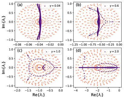
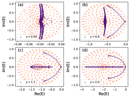
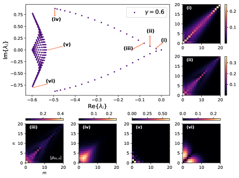
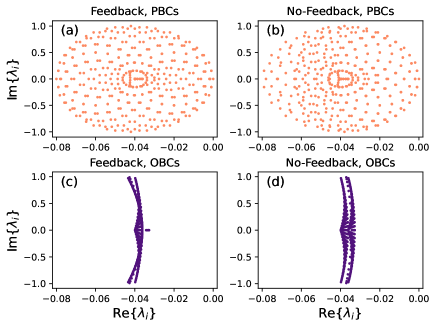
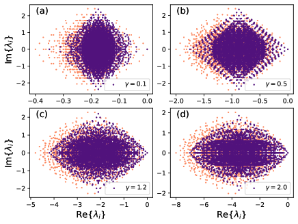
As show in Fig. 1, the Liouvillian spectrum under PBCs is totally different from OBCs, which is reminiscent of distinct energy spectrum under PBCs and OBCs for non-Hermitian Hamiltonian hosting NHSE. Indeed, there is deep connection between the Liouvillian spectrum and energy spectrum of the effective non-Hermitian Hamiltonian for the model in this paper, which is directly reflected by the perturbation analysis in Appendix A. We will briefly illustrate it in the following.
For the feedback case under PBCs, we observe that , enabling us to take as the unperturbed part. Its corresponding eigenmodes are the zeroth-order eigenmodes of the whole Liouvillian superoperator , with denoting Bloch waves with crystal momentum . The resultant zeroth-order eigenvalues are expressed as . Moreover, the first and second-order corrections of eigenvalues are about , so for large system size , the border of PBCs Liouvillian spectrum is well characterized by . For example, zeroth-order eigenvalues set the restrictions and , which agree well with the numerical results. Furthermore, as shown in Fig. S1 of Appendix. A, we also consider the first-order corrections of eigenvalues, which are more close to the numerical results (see Fig. 1(a)) of exact diagonalization.
On the other hand, under OBCs, a similar perturbation analysis is performed in Appendix. A.2. In contrast with PBCs, the effective non-Hermitian Hamiltonian exhibits NHSE under OBCs, implying that its eigenstates are exponentially localized instead of extended Bloch waves. Neglecting two terms of unperturbed Liouvillian (see Appendix. A.2), the zeroth-order Liouvillian eigenvalues roughly take the form
| (6) | ||||
in which , . Although the approximation is pretty loosely, indeed explains some properties of OBCs Liouvillian spectrum. For instance, when , as depicted in Fig. 1(a),(b), a large proportion of eigenvalues are located around , with the imaginary part of eigenvalues approximately following . Moreover, when , the eigenvalue is hugely degenerate. As for , most eigenvalues tend to reside on the real axis. These observations can be directly interpreted to some extent using Eq. 6. However, there are many features of OBCs Liouvillian spectrum beyond the scope of zeroth-order approximation (i.e. Eq. 6). Therefore, as shown in Fig. S1(c), we also include the first-order corrections of eigenvalues, which already roughly provide correct shape of Liouvillian spectrum displayed in Fig. 1. Furthermore, it is reasonable to predict that higher corrections will further improve the accuracy. In summary, our perturbation analysis reveals that the sensitivity of the Liouvillian spectrum is originated from the sensitivity of the energy spectrum of the non-Hermitian effective Hamiltonian.
IV.1.2 steady state
As proved in Appendix A.1, under PBCs, the steady state can be exactly determined as
| (7) |
in which and . This steady state is nontrivial, since it is highly coherent. In particular, for , , which means the absolute value of all elements of is equal to . However, it is common for an open quantum system to undergo decoherence and reach an incoherent steady state finally. Therefore, we attribute this coherent steady state to the intricate interplay between unitary evolution, continuous measurements and special feedback operations.
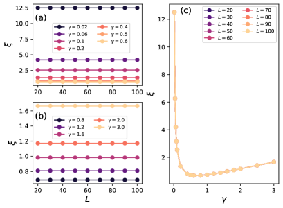
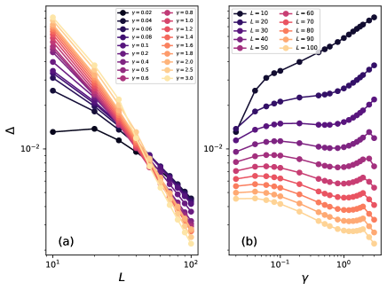
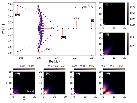
As for OBCs, an analytical form of steady state is absent. Nevertheless, our perturbation theory suggests that the majority of Liouvillian eigenmodes will tend to be localized due to the exponential localization behavior of ’s eigenstates. We numerically acquire the steady state under OBCs, whose off diagonal elements are almost zero. Moreover, the diagonal elements exhibits exponential localization behaviors similar to the Hatano-Nelson model (i.e. ). Therefore, we extract the localization length through fitting the diagonal elements of steady state . As shown in Fig. 2, the localization length initially experiences a rapid decline with increasing when . However, once , the localization length smoothly increases with growing . Furthermore, as depicted in Fig. 2, the localization length is independent of system size . These observed behaviors closely resemble those exhibited by the Hatano-Nelson model.
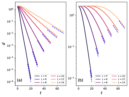
The preceding analysis indicates that the Liouvillian spectrum and Liouvillian eigenmodes, including the steady state, are greatly altered when changing boundary conditions. In the subsequent section, we delve into a detailed investigation of the distinct relaxation processes under both PBCs and OBCs. To quantify relaxation time , we evaluate distance , in which . We define relaxation time as the smallest time at which .
IV.1.3 Liouvillian gap and relaxation dynamics
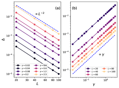
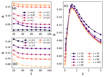
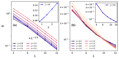
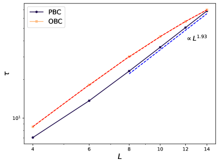
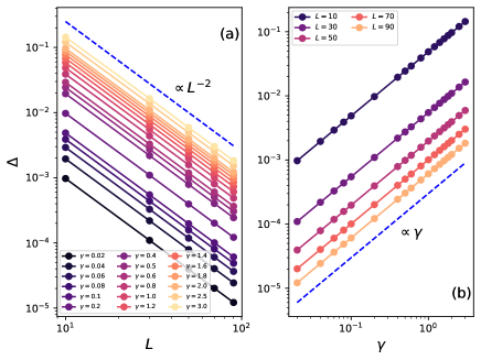
Before discussing relaxation time , we firstly calculate the scaling relation between Liouvillian gap and system size . As illustrated in Fig. 3, we find good scaling relations and under PBCs. These scaling relations under PBCs are well explained by perturbation theory in Appendix. A.1, from which the Liouvillian gap approximately satisfies . On the contrary, as shown in Fig. 4, for arbitrary , Liouvillian gap remains finite with the increase in system size under OBCs. Additionally, for systems with various size , with the increase in , Liouvillian gap initially increases and then decreases.
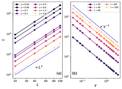
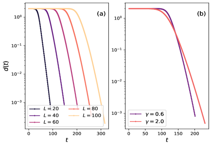
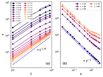
As for relaxation time, we find the relaxation time follows the usual law under PBCs. Specifically, as indicated in Fig. 5(a) and (b), the relaxation time exhibits scaling behaviors of and , respectively. Moreover, as shown in Fig. S5, another evidence is that distance under PBCs immediately decays as the manner controlled by the inverse of Liouvillian gap, thus inferring .
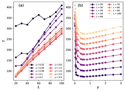
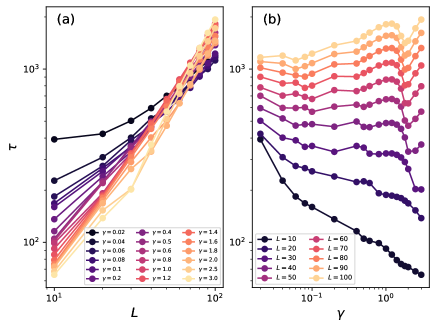
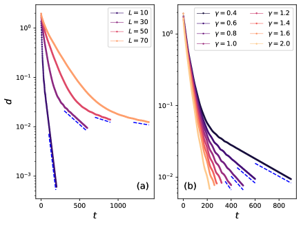
When switching into OBCs, as shown in Fig. 6(a), the relaxation time is approximately proportional to . However, for small , such as , deviates from the relation , which is finite-size effect. Because the localization length is comparable with system size when is sufficiently small and . Moreover, as depicted in Fig. 6(b), the minimum relaxation time occurs around , at which the steady state displays the strongest LSE. Therefore, we can infer that the Liouvillian skin effect can help shorten the relaxation time. A previous work has unveiled similar scaling relation between relaxation time and system size (), despite the much difference between our Lindbladians and theirs[15]. This anomalous scaling relation under OBCs can be primarily attributed to the LSE of the first eigenmodes and . The corresponding coefficient follows , in which is approximately because of the exponential localization of and (see Fig. S2). Therefore, the relaxation time should approximately obey , leading to [15]. In the thermodynamic limit, since Liouvillian gap is finite, the second term will dominate, yielding .
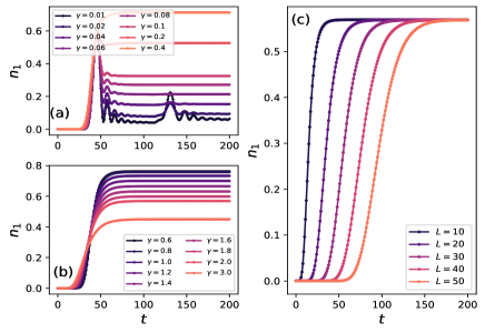
In addition to distance , we also directly observe the evolution of the density at the first site and the last site to gain the intuitive pictures for different scaling behaviors of relaxation time. We imagine the initial state as a “particle” situated at site . Under OBCs, we observe the evolution of density at the first site. When , remains zero until the “particle” moves to the left, after which the density rapidly reaches a maximum value and remains constant, which means the “particle” is sticky to the edge once the “particle” touches the boundary. However, for , after reaching the peak, begins to fall down, suggesting partial reflection of the “particle”. When is very small, the evolution of density resembles the unitary case with , in which will constantly irregularly oscillate. For example, for or , it should undergo several oscillations until finally reaches the steady state, so the relaxation time is significantly longer than the big cases as indicated in Fig. 6(b). Furthermore, for , it’s shown in Fig. 7(b), the relaxation time for is relatively insensitive to at least for small sizes, aligning with the results in Fig. 6(b). Moreover, as illustrated in Fig. 7(c), the relaxation time is proportional to system size , which makes sense since the propagation “velocity” is finite due to the Lieb-Robinson bound[68, 69]. Therefore, it always takes at least time for “particle” to move through the whole bulk.
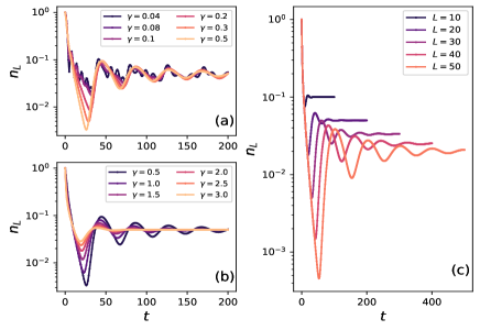
In contrast, the relaxation dynamics under PBCs differs significantly from the case under OBCs. As depicted in Fig. 8, compared with the OBCs case, the observable undergoes numerous oscillation periods before reaching the steady state. Notably, larger monitoring lead to shorter oscillatory periods. Specifically, as shown in Fig. 8(c), for and , the time of the first peaks of under PBCs are approximately , which indicates the period linearly grows . Moreover, the system should undergo about periods before reaching the steady state. We observe is approximately proportional to , so the relaxation time under PBCs follows .
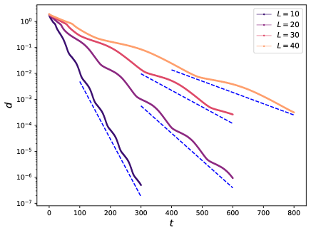
Interestingly, for the single-particle case under OBCs, we observe the cutoff phenomena, indicating that relaxation does not occur until a certain time, after which it rapidly proceeds with in a time window of . To be concrete, as depicted in Fig. 9, distances remain constant up to a considerable time () before rapidly decreasing. This phenomenon can be attributed to the steady state being close to , while the initial state is , ensuring the state “far from” the steady state for a considerable time during evolution. A straightforward calculation is that . The approximation relies on the fact that if the initial state is away from , then and will keep close to zero for a while, as takes time to gradually approach . Hence, it is clear that cutoff phenomena depend on initial state. For instance, given a uniform initial state, then , implying that cutoff phenomenon will disappear. Additionally, as depicted in Fig. 9(b), the duration for which the distance remains constant increases with the strength of the skin effect. Conversely, under PBCs, the cutoff phenomenon is absent due to the delocalized structure of . Moreover, cutoff phenomenon provide us another viewpoint to intuitively understand the scaling behavior , which can be divided into two parts . As depicted in Fig. 9, the first part is that distance keeps unchanged for a duration , and the second part is that distance roughly exponentially decays as the inverse of Liouvillian gap, thus resulting in .
IV.2 Many-body case
In this section, we briefly explore the Lindbladian with feedback under OBCs in the many-body half-filled sector. The aim is to see the relaxation behaviors of many-body LSE.
Due to exponential growth of dimensions of the Liouvillian superoperator for the many-body case, the exact diagonalization is limited to very small system size . Therefore, besides exact diagonalization, we also employ the quantum jump method to simulate the evolution, enabling us to obtain the evolution of the density distribution. The numerical implementations have been elucidated in previous works[70, 60, 61].
IV.2.1 Many-body Liouvillian skin effect
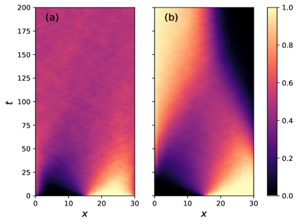
As shown in Fig. 10(b), the steady state under OBCs exhibits the many-body LSE, which represents that almost all of particles are localized at the left half side, leaving the right half side nearly empty. Previous studies have proved that many-body LSE immensely suppress the entanglement growth, driving the system into area law phase for any nonzero . This effect arises because most of the particles become frozen due to the Pauli exclusion principle, while only fluctuation areas around the middle contribute to the generation of entanglement[60, 61].
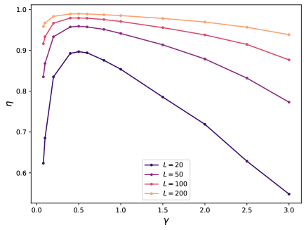
For many-body cases, to quantify the strength of skin effect, we define
| (8) |
where and represent the number of particles on the left and right halves, respectively. Obviously, the larger the is, the stronger the skin effect is. The density distribution is uniform for , while particles are entirely localized on the left side for .
Interestingly, the many-body LSE bears some resemblance to the single-body LSE. Specifically, as depicted in the Fig. 11, is maximum when is around 0.5, in which the localization length is approximately minimum for the single-body case. In other words, is roughly corresponding to the strongest LSE for both single-body and many-body cases. In addition, when is small, the slope is steeper, whereas for larger , the slope is smoother, agreeing with the behavior observed in the single-body case. However, for the many-body case, will increase with system size and we suspect that will always equal one in the thermodynamics’s limit. We argue that it is because the middle fluctuation zone is , thus the proportion of frozen areas, namely completely occupied or unoccupied zone, increases with [61]. The corresponding single-body picture is that localization length is independent of , so the particle will always be completely localized in the left half side for sufficiently large .
IV.2.2 Relaxation dynamics
Firstly, we perform exact diagonalization for the half-filled case up to . As Fig. 12(a) shows, under PBCs, we find the Liouvillian gap approximately scale as and displays a nearly linear growth with . In contrast, under OBCs, the Liouvillian gap decreases with the system size , along with the decreasing slope. Consequently, it is reasonable to predict that Liouvillian gap under OBCs will keep finite in the thermodynamic limit. In conclusion, the many-body finite-size results of Liouvillian gap are consistent with the single-body results.
As shown in Fig. 13, the relaxation time under PBCs roughly obeys , which approximately satisfies . However, this simple relation between relaxation time and Liouvillian gap fails under OBCs, analogous to the single-particle case. As Fig. 13 shows, the exponent in under OBCs constantly decreases with within the range of that we are capable to calculate. We suspect that the relaxation time will still behave as in the thermodynamic limit. Furthermore, Fig 14 indicates that the cutoff phenomenon still persists in the many-body context under OBCs. Although the Liouvillian gap gives the correct asymptotic decay rate (blue dotted line), the crossover time to get into the asymptotic regime diverges with system size , as shown in Fig. 14(b).
V Lindbladian Without Feedback
In the above section, we have already studied the Lindbladian with feedback, which supports a current-carrying steady state under PBCs and exhibits LSE in the steady state under OBCs. In this section, we turn to investigate the Lindbladian without feedback, namely Lindblad operators are given by . Without feedback, the Lindblad operators are Hermitian, so the maximally mixed state must be one steady state. However, the situation seems more intricate under PBCs. As proved in Appendix. A.3, when the system size , there exists bistable steady states, one is , the other is . It is evident that any linear combinations of and is steady state as well. In general, bistable steady states can significantly influence the relaxation process. For example, given different initial states, the system can evolve into different steady states. For simplicity, we will not discuss the dynamical effect caused by bistable steady states. In comparison, under OBCs, the steady state is just the maximally mixed state regardless of system size .
V.1 Sensitive of boundary condition
Interestingly, even though the steady state is free from skin effect for the no-feedback case, Liouvillian spectrum, Liouvillian eigenmodes and relaxation dynamics are still sensitive to boundary conditions.
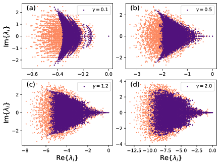
As shown in Fig. 15, the Liouvillian spectrum differs between PBCs and OBCs. The shapes of Liouvillian spectra can also be roughly explained by perturbation theory, similar with the feedback case (see Appendix. A.3, A.4 and Fig. S1). Besides the whole Liouvillian spectrum, the Liouvillian gap , namely the real part of first nonzero Liouvillian eigenvalue , is also sensitive to boundary conditions. As shown in Fig. 16, the Liouvillian gap exhibits good scaling behaviors as and under PBCs, the same with the feedback case under PBCs. In contrast, as illustrated in Fig. 17, the Liouvillian gap is irregular under OBCs. Moreover, we find that for no-feedback case under OBCs always has a nonzero imaginary part, which explains the fluctuation of the distance in Fig. S6.
As for eigenmodes, as indicated in Fig. 18, apart from the steady state and a few eigenmodes around the steady state, the majority of Liouvillian eigenmodes exhibit LSE, which is the signal of the sensitivity. It is consistent with the perturbation analysis, from which we know the zeroth-order solutions display skin effect. Moreover, we also compare the eigenmodes for no-feedback case under OBCs (see Fig. 18) with the eigenmodes for feedback case under OBCs (see Fig. S2). As a comparison, for the latter, its steady state and eigenmodes around steady states also exhibit strong LSE. This difference leads to completely distinct relaxation behaviors for Lindbladian with feedback and without feedback under OBCs.
V.2 Relaxation behaviors
Due to the sensitivity of Liouvillian spectrum and Liouvillian eigenmodes, it is natural to expect that the relaxation time is also sensitive to boundary conditions. Indeed, as shown in Fig. 19 and 20, the relaxation time is greatly altered when changing boundary conditions.
Interestingly, for the Lindbladian without feedback under PBCs, we find the relaxation time is much shorter than the inverse of the Liouvillian gap. Specifically speaking, the numerical results (see Fig. 19 (a)) indicate , while the inverse of the Liouvillian gap gives . Moreover, the relaxation time will also deviate from as shown in Fig. 19(b). These phenomenon stems from the accelerated relaxation in the transient regime. As shown in Fig. 21, before entering the asymptotic regime determined by Liouvillian gap , the system undergoes faster relaxing process for a long time. This transient regime takes up a large part for the overall relaxation process, so the faster relaxation rate in the transient regime will greatly decrease the relaxation time and lead to . A recent study explains the accelerated relaxation phenomenon in bulk-dissipative system from the operator spreading, which deserves further research[17, 71]. As for the Lindbladian without feedback under PBCs, the faster relaxation has a simple reason. Numerically, we find that , which means other higher eigenmodes, such as , , …, also play an important role in the relaxation process, thus resulting in faster decay of distance. In contrast, for no-feedback case under OBCs, , implying that the is the dominant term for relaxations.
For the Lindbladian without feedback under OBCs, we find that the relaxation time is again controlled by the inverse of Liouvillian gap . Firstly, we have numerically checked the scaling behavior of relaxation time in Fig. 20, which is well fitted with the inverse of Liouvillian gap in Fig. 17 for various . Another evidence is to observe the evolution of distance (see Fig. S6). We discover that the distance immediately decays in the manner controlled by Liouvillian gap , and the fluctuation of distance is caused by the imaginary part of . Physically, it is reasonable since the steady state and low Liouvillian eigenmodes are free from skin effect. Therefore, the coefficients of eigenmodes around the steady state are still finite, although the coefficients of high eigenmodes can be exponentially large. After a short time, the relaxation process is dominated by , and thus leading to . Moreover, the relation between the relaxation time and monitoring rate under OBCs is non-monotonic, while the relaxation time under PBCs always decreases with .
VI Conclusion and Outlook
In summary, we have investigated the Liouvillian spectrum, eigenmodes, and relaxation dynamics of two Lindbladians, which share the same non-Hermitian effective Hamiltonian. We find both Lindbladians are sensitive to boundary conditions due to LSE, which is originated from the NHSE of non-Hermitian effective Hamiltonian. When changing the boundary conditions, the Liouvillian spectrum, Liouvillian eigenmodes and relaxation dynamics are all dramatically altered.
To be specific, we list the main results as follows: (i) For the Lindbladian with feedback under PBCs, the steady state is highly coherent and eigenmodes are extended. The relaxation time is controlled the inverse of the Liouvillian gap and scales as . (ii) For the Lindbladian with feedback under OBCs, because the corresponding Lindbladian under PBCs carries current in the steady state, the steady state will be localized under OBCs. In other words, the eigenmodes including the steady state exhibit LSE, which is able to lead to cutoff phenomenon. Moreover, the LSE of low eigenmodes, especially for , can result in exponentially large coefficients . As a consequence, the relaxation time obeys , implying in the thermodynamic limit. Our finite-size results support that the LSE and distinct scaling relations between relaxation time and system size under PBCs and OBCs still hold in many-body system. (iii) For the Lindbladian without feedback under PBCs, we find if system size , the steady state is the unique maximally mixed state . Interestingly, if the system size , there exists bistable steady states, one is and another is . Moreover, the eigenmodes are extended due to the translation invariance. Remarkably, we observe that the relaxation time () is smaller than the inverse of the Liouvillian gap (), which stems from the faster relaxation persisting for a long time in the transient regime before entering the asymptotic regime governed by the Liouvillian gap. (iv) For the Lindbladian without feedback under OBCs, although the majority of eigenmodes exhibit LSE, the steady state and a few eigenmodes around steady state are extended. Moreover, we find the eigenmodes and dominate the decay of the distance immediately, which implies that the relaxation time follows . Consequently, the relaxation time scales as , in which is the same scaling exponent of the Liouvillian gap . Moreover, the relation between relaxation time and monitoring rate is also dramatically altered when changing boundary conditions. Roughly speaking, for both Lindbladians with feedback and without feedback under PBCs, the relaxation time decreases with , while the relaxation time presents non-monotonic dependence on under OBCs.
Our work investigates two typical symmetric boundary-sensitive Lindbladians, whose sensitivity originates from Liouvillian skin effect. There are several interesting directions which merit further study. First of all, it remains unclear whether the single-particle relaxation behaviors still generally hold in many-body case? Secondly, it is tempting to construct other boundary sensitive Lindbladians beyond skin effect. For example, the topological edge mode under OBCs can also dramatically alter the relaxation properties[11]. Another direction is to investigate the nontrivial dynamics induced by the interplay of the Anderson localization and the skin effect[72, 73]. It is reasonable to predict the Anderson localization will compete with skin effect and may enrich the relaxation dynamics. Lastly, our work shows that Lindbladians with current-carrying steady state and Lindbladians with no-current steady state exhibit different relaxation behaviors. So, it is worthwhile to investigate the dynamics of other Lindbladians hosting current-carrying steady state, such as asymmetric exclusion process[74], and uncover possible universal laws.
Acknowledgements.
We thank Shuo, Liu for helpful discussions. The work is supported by National Key Research and Development Program of China (Grant No. 2021YFA1402104), the NSFC under Grants No.12174436 and No.T2121001 and the Strategic Priority Research Program of Chinese Academy of Sciences under Grant No. XDB33000000.References
- Breuer and Petruccione [2007] H.-P. Breuer and F. Petruccione, The Theory of Open Quantum Systems (Oxford University Press, 2007).
- Wiseman and Milburn [2009] H. M. Wiseman and G. J. Milburn, Quantum Measurement and Control (Cambridge University Press, 2009).
- Barreiro et al. [2011] J. T. Barreiro, M. Müller, P. Schindler, D. Nigg, T. Monz, M. Chwalla, M. Hennrich, C. F. Roos, P. Zoller, and R. Blatt, An open-system quantum simulator with trapped ions, Nature 470, 486 (2011).
- Cai and Barthel [2013] Z. Cai and T. Barthel, Algebraic versus exponential decoherence in dissipative many-particle systems, Phys. Rev. Lett. 111, 150403 (2013).
- Diehl et al. [2008] S. Diehl, A. Micheli, A. Kantian, B. Kraus, H. P. Büchler, and P. Zoller, Quantum states and phases in driven open quantum systems with cold atoms, Nature Physics 4, 878 (2008).
- Diehl et al. [2011] S. Diehl, E. Rico, M. A. Baranov, and P. Zoller, Topology by dissipation in atomic quantum wires, Nature Physics 7, 971 (2011).
- Sieberer et al. [2016] L. M. Sieberer, M. Buchhold, and S. Diehl, Keldysh field theory for driven open quantum systems, Reports on Progress in Physics 79, 096001 (2016).
- Verstraete et al. [2009] F. Verstraete, M. M. Wolf, and J. Ignacio Cirac, Quantum computation and quantum-state engineering driven by dissipation, Nature Physics 5, 633 (2009).
- Weimer et al. [2010] H. Weimer, M. Müller, I. Lesanovsky, P. Zoller, and H. P. Büchler, A rydberg quantum simulator, Nature Physics 6, 382 (2010).
- Lindblad [1976] G. Lindblad, On the generators of quantum dynamical semigroups, Communications in Mathematical Physics 48, 119 (1976).
- Vernier [2020] E. Vernier, Mixing times and cutoffs in open quadratic fermionic systems, SciPost Phys. 9, 049 (2020).
- Zhou et al. [2022] B. Zhou, X. Wang, and S. Chen, Exponential size scaling of the liouvillian gap in boundary-dissipated systems with anderson localization, Phys. Rev. B 106, 064203 (2022).
- Žnidarič [2015] M. Žnidarič, Relaxation times of dissipative many-body quantum systems, Phys. Rev. E 92, 042143 (2015).
- Mori and Shirai [2020] T. Mori and T. Shirai, Resolving a discrepancy between liouvillian gap and relaxation time in boundary-dissipated quantum many-body systems, Phys. Rev. Lett. 125, 230604 (2020).
- Haga et al. [2021] T. Haga, M. Nakagawa, R. Hamazaki, and M. Ueda, Liouvillian skin effect: Slowing down of relaxation processes without gap closing, Phys. Rev. Lett. 127, 070402 (2021).
- Wang et al. [2023] Z. Wang, Y. Lu, Y. Peng, R. Qi, Y. Wang, and J. Jie, Accelerating relaxation dynamics in open quantum systems with liouvillian skin effect, Phys. Rev. B 108, 054313 (2023).
- Mori and Shirai [2023] T. Mori and T. Shirai, Symmetrized liouvillian gap in markovian open quantum systems, Phys. Rev. Lett. 130, 230404 (2023).
- Yao and Wang [2018] S. Yao and Z. Wang, Edge states and topological invariants of non-hermitian systems, Phys. Rev. Lett. 121, 086803 (2018).
- Xiao et al. [2020] L. Xiao, T. Deng, K. Wang, G. Zhu, Z. Wang, W. Yi, and P. Xue, Non-hermitian bulk–boundary correspondence in quantum dynamics, Nature Physics 16, 761 (2020).
- Zhang et al. [2020] K. Zhang, Z. Yang, and C. Fang, Correspondence between winding numbers and skin modes in non-hermitian systems, Phys. Rev. Lett. 125, 126402 (2020).
- Okuma et al. [2020] N. Okuma, K. Kawabata, K. Shiozaki, and M. Sato, Topological origin of non-hermitian skin effects, Phys. Rev. Lett. 124, 086801 (2020).
- Lee and Thomale [2019] C. H. Lee and R. Thomale, Anatomy of skin modes and topology in non-hermitian systems, Phys. Rev. B 99, 201103(R) (2019).
- Borgnia et al. [2020] D. S. Borgnia, A. J. Kruchkov, and R.-J. Slager, Non-hermitian boundary modes and topology, Phys. Rev. Lett. 124, 056802 (2020).
- Yokomizo and Murakami [2019] K. Yokomizo and S. Murakami, Non-bloch band theory of non-hermitian systems, Phys. Rev. Lett. 123, 066404 (2019).
- Yang et al. [2020] Z. Yang, K. Zhang, C. Fang, and J. Hu, Non-hermitian bulk-boundary correspondence and auxiliary generalized brillouin zone theory, Phys. Rev. Lett. 125, 226402 (2020).
- Guo et al. [2021] C.-X. Guo, C.-H. Liu, X.-M. Zhao, Y. Liu, and S. Chen, Exact solution of non-hermitian systems with generalized boundary conditions: Size-dependent boundary effect and fragility of the skin effect, Phys. Rev. Lett. 127, 116801 (2021).
- Li et al. [2020] L. Li, C. H. Lee, S. Mu, and J. Gong, Critical non-hermitian skin effect, Nature communications 11, 1 (2020).
- Zhang et al. [2022] K. Zhang, Z. Yang, and C. Fang, Universal non-hermitian skin effect in two and higher dimensions, Nature Communications 13, 2496 (2022).
- Wang et al. [2022a] H.-Y. Wang, F. Song, and Z. Wang, Amoeba formulation of the non-hermitian skin effect in higher dimensions, arXiv:2212.11743 (2022a).
- Hu [2023] H. Hu, Non-hermitian band theory in all dimensions: uniform spectra and skin effect, arXiv:2306.12022 (2023).
- Alsallom et al. [2022] F. Alsallom, L. Herviou, O. V. Yazyev, and M. Brzezińska, Fate of the non-hermitian skin effect in many-body fermionic systems, Phys. Rev. Research 4, 033122 (2022).
- Kawabata et al. [2019] K. Kawabata, K. Shiozaki, M. Ueda, and M. Sato, Symmetry and topology in non-hermitian physics, Phys. Rev. X 9, 041015 (2019).
- Ashida et al. [2020] Y. Ashida, Z. Gong, and M. Ueda, Non-hermitian physics, Advances in Physics 69, 249 (2020).
- Bergholtz et al. [2021] E. J. Bergholtz, J. C. Budich, and F. K. Kunst, Exceptional topology of non-hermitian systems, Rev. Mod. Phys. 93, 015005 (2021).
- Lin et al. [2023] R. Lin, T. Tai, L. Li, and C. H. Lee, Topological non-hermitian skin effect, Frontiers of Physics 18, 53605 (2023).
- Okuma and Sato [2023] N. Okuma and M. Sato, Non-hermitian topological phenomena: A review, Annual Review of Condensed Matter Physics 14, 83 (2023).
- Song et al. [2019] F. Song, S. Yao, and Z. Wang, Non-hermitian skin effect and chiral damping in open quantum systems, Phys. Rev. Lett. 123, 170401 (2019).
- Liu et al. [2020] C.-H. Liu, K. Zhang, Z. Yang, and S. Chen, Helical damping and dynamical critical skin effect in open quantum systems, Phys. Rev. Res. 2, 043167 (2020).
- Yang et al. [2022] F. Yang, Q.-D. Jiang, and E. J. Bergholtz, Liouvillian skin effect in an exactly solvable model, Phys. Rev. Res. 4, 023160 (2022).
- Li and Wan [2022] H. Li and S. Wan, Dynamic skin effects in non-hermitian systems, Phys. Rev. B 106, L241112 (2022).
- Kawabata et al. [2023] K. Kawabata, T. Numasawa, and S. Ryu, Entanglement phase transition induced by the non-hermitian skin effect, Phys. Rev. X 13, 021007 (2023).
- Sawada et al. [2023] T. Sawada, K. Sone, R. Hamazaki, Y. Ashida, and T. Sagawa, Role of topology in relaxation of one-dimensional stochastic processes, arXiv:2301.09832 (2023).
- McDonald et al. [2022] A. McDonald, R. Hanai, and A. A. Clerk, Nonequilibrium stationary states of quantum non-hermitian lattice models, Phys. Rev. B 105, 064302 (2022).
- Li et al. [2023a] B. Li, H.-R. Wang, F. Song, and Z. Wang, Non-bloch dynamics and topology in a classical non-equilibrium process, arXiv:2306.11105 (2023a).
- Fleckenstein et al. [2022] C. Fleckenstein, A. Zorzato, D. Varjas, E. J. Bergholtz, J. H. Bardarson, and A. Tiwari, Non-hermitian topology in monitored quantum circuits, Phys. Rev. Res. 4, L032026 (2022).
- Skinner et al. [2019] B. Skinner, J. Ruhman, and A. Nahum, Measurement-induced phase transitions in the dynamics of entanglement, Phys. Rev. X 9, 031009 (2019).
- Li et al. [2018] Y. Li, X. Chen, and M. P. A. Fisher, Quantum zeno effect and the many-body entanglement transition, Phys. Rev. B 98, 205136 (2018).
- Li et al. [2019] Y. Li, X. Chen, and M. P. A. Fisher, Measurement-driven entanglement transition in hybrid quantum circuits, Phys. Rev. B 100, 134306 (2019).
- Chan et al. [2019] A. Chan, R. M. Nandkishore, M. Pretko, and G. Smith, Unitary-projective entanglement dynamics, Phys. Rev. B 99, 224307 (2019).
- Liu et al. [2023] S. Liu, M.-R. Li, S.-X. Zhang, S.-K. Jian, and H. Yao, Universal kardar-parisi-zhang scaling in noisy hybrid quantum circuits, Phys. Rev. B 107, L201113 (2023).
- Cao et al. [2019] X. Cao, A. Tilloy, and A. D. Luca, Entanglement in a fermion chain under continuous monitoring, SciPost Phys. 7, 024 (2019).
- Alberton et al. [2021] O. Alberton, M. Buchhold, and S. Diehl, Entanglement transition in a monitored free-fermion chain: From extended criticality to area law, Phys. Rev. Lett. 126, 170602 (2021).
- Turkeshi et al. [2021] X. Turkeshi, A. Biella, R. Fazio, M. Dalmonte, and M. Schiró, Measurement-induced entanglement transitions in the quantum ising chain: From infinite to zero clicks, Phys. Rev. B 103, 224210 (2021).
- Gullans and Huse [2020] M. J. Gullans and D. A. Huse, Dynamical purification phase transition induced by quantum measurements, Phys. Rev. X 10, 041020 (2020).
- Buchhold et al. [2022] M. Buchhold, T. Müller, and S. Diehl, Revealing measurement-induced phase transitions by pre-selection, arXiv:2208.10506 (2022).
- O’Dea et al. [2022] N. O’Dea, A. Morningstar, S. Gopalakrishnan, and V. Khemani, Entanglement and absorbing-state transitions in interactive quantum dynamics, arXiv:2211.12526 (2022).
- Ravindranath et al. [2023a] V. Ravindranath, Y. Han, Z.-C. Yang, and X. Chen, Entanglement steering in adaptive circuits with feedback, Phys. Rev. B 108, L041103 (2023a).
- Ravindranath et al. [2023b] V. Ravindranath, Z.-C. Yang, and X. Chen, Free fermions under adaptive quantum dynamics, arXiv:2306.16595 (2023b).
- Sierant and Turkeshi [2023] P. Sierant and X. Turkeshi, Controlling entanglement at absorbing state phase transitions in random circuits, Phys. Rev. Lett. 130, 120402 (2023).
- Wang et al. [2022b] Y.-P. Wang, C. Fang, and J. Ren, Absence of entanglement transition due to feedback-induced skin effect, arXiv:2209.11241 (2022b).
- Feng et al. [2023] X. Feng, S. Liu, S. Chen, and W. Guo, Absence of logarithmic and algebraic scaling entanglement phases due to the skin effect, Physical Review B 107, 094309 (2023).
- Hamanaka et al. [2023] S. Hamanaka, K. Yamamoto, and T. Yoshida, Interaction-induced liouvillian skin effect in a fermionic chain with a two-body loss, Phys. Rev. B 108, 155114 (2023).
- Li et al. [2023b] H. Li, H. Wu, W. Zheng, and W. Yi, Many-body non-hermitian skin effect under dynamic gauge coupling, Phys. Rev. Res. 5, 033173 (2023b).
- Hatano and Nelson [1996] N. Hatano and D. R. Nelson, Localization transitions in non-hermitian quantum mechanics, Phys. Rev. Lett. 77, 570 (1996).
- Barthel and Zhang [2022] T. Barthel and Y. Zhang, Solving quasi-free and quadratic lindblad master equations for open fermionic and bosonic systems, Journal of Statistical Mechanics: Theory and Experiment 2022, 113101 (2022).
- Choi [1975] M.-D. Choi, Completely positive linear maps on complex matrices, Linear Algebra and its Applications 10, 285 (1975).
- Jamiołkowski [1972] A. Jamiołkowski, Linear transformations which preserve trace and positive semidefiniteness of operators, Reports on Mathematical Physics 3, 275 (1972).
- Lieb and Robinson [1972] E. H. Lieb and D. W. Robinson, The finite group velocity of quantum spin systems, Communications in Mathematical Physics 28, 251 (1972).
- Poulin [2010] D. Poulin, Lieb-robinson bound and locality for general markovian quantum dynamics, Phys. Rev. Lett. 104, 190401 (2010).
- Daley [2014] A. J. Daley, Quantum trajectories and open many-body quantum systems, Advances in Physics 63, 77 (2014).
- Shirai and Mori [2023] T. Shirai and T. Mori, Accelerated decay due to operator spreading in bulk-dissipated quantum systems, arXiv:2309.03485 (2023).
- Jiang et al. [2019] H. Jiang, L.-J. Lang, C. Yang, S.-L. Zhu, and S. Chen, Interplay of non-hermitian skin effects and anderson localization in nonreciprocal quasiperiodic lattices, Phys. Rev. B 100, 054301 (2019).
- Li et al. [2023c] K. Li, Z.-C. Liu, and Y. Xu, Disorder-induced entanglement phase transitions in non-hermitian systems with skin effects, arXiv:2305.12342 (2023c).
- Derrida [1998] B. Derrida, An exactly soluble non-equilibrium system: The asymmetric simple exclusion process, Physics Reports 301, 65 (1998).
Appendix A Perturbation theory of Lindbladians
A.1 With feedback, PBCs
In this section, we investigate the Lindbladian with feedback under PBCs. The discussion will be restricted in the single-particle sector. The Hamiltonian is given as . Moreover, the Lindblad operators are and .
A.1.1 Liouvillian spectrum and gap
Firstly, it can be easily verified , so and will share common eigenstates. By virtue of this property, we decompose the Lindbladian into two parts: . and are respectively as follows:
| (S1) | ||||
in which and . For the translation invariant free fermion Hamiltonian , we can perform Fourier transformation , and thus can be rewritten as , in which , . and are equivalent, if they differ by integer multiples of 2. Obviously, are right eigenvectors of the Liouvillian , satisfying , namely the zeroth-order eigenvalues are . Utilizing the perturbation theory, the first-order corrections of eigenvalues can be obtained as follows:
| (S2) | ||||
Furthermore, the second-order corrections of eigenvalues take the form
| (S3) | ||||
in which and . Then substituting into the above equation, the Eq. S3 is reduced to
| (S4) |
The eigenvalues are approximated as . In general, for relatively large , because both and are about , . In other words, Liouvillian spectrum is dominated by . Therefore, the real and imaginary part of Liouvillian spectrum are and , respectively, which is consistent with Fig. 1, which shows and .
The first-order perturbation of the eigenvectors is
| (S5) | ||||
Obviously, the first-order correction of eigenvector . Moreover, the zeroth-order and higher order eigenvalues for satisfy . Therefore, it’s straightforward to speculate that is the steady state for the whole Lindbladian and indeed we can readily verify it later.
The first and second-order perturbation analysis above is restricted in non-degenerate case. Besides non-degenerate zeroth-order eigenvalues, there are also and zeroth-order eigenvalues, whose degeneracies are 2 and , respectively. For instance, is -fold degenerate, and is two-fold degenerate (degenerate with ). According to degenerate perturbation theory, assume is degenerate with , the corresponding first-order correction of eigenvalues is given by
| (S6) | ||||
in which . For -fold degenerate case, the first-order corrections of eigenvalues follow
| (S7) |
in which . The first-order perturbation results are shown in Fig. S1(a).
A.1.2 steady state
As mentioned above, the steady state is corresponding to . The Liouvillian gap , aligning with Fig. 3. Specifically, the unique steady state takes the form
| (S8) | ||||
which is highly coherent. However, steady state should maintain periodicity, which demands , namely , . Another evidence is that can be exactly chosen only when .
In comparison, for , , it is known that , , so , thus will not be steady state. However, from the perturbation results, it is justifiable to assume that the steady state takes the form . Therefore, the steady state is required to obey , which can be simplified as
| (S9) | ||||
According to the Eq. S9, it can be readily inferred that .
So, in general, the steady state is , . When , all equal zero except , which is consistent with Eq. S8.
A.2 With feedback, OBCs
In this section, we also perform the perturbation analysis for the feedback case under OBCs, which elucidates the Lindbladians’ extreme sensitivity of boundary conditions and the localization of eigenmodes under OBCs. For feedback case under OBCs, the Hamiltonian is expressed as and the effective non-Hermitian is given by .
A.2.1 Liouvillian spectrum
Likewise, we can perform the same decomposition of the Lindbladian as Appendix. A.1, namely , in which and the perturbed part is . The effective non-Hermitian Hamiltonian is . Neglecting the terms of , the right eigenvectors of are approximate to , while the left eigenvectors of are approximately as . The right and left eigenvectors satisfy biorthogonal relation . Consequently, we can obtain for , while for . Therefore, the zeroth-order eigenvalues of the Lindbladian are approximately
| (S10) | ||||
The approximate zeroth-order eigenvalues of the Liouvillian roughly tells that for , the Liouvillian eigenvalues will satisfy , which is roughly fitted with Fig. 1(a), and for , the Liouvillian eigenvalues should satisfy , which is also approximately consistent with Fig. 1(d), where most of eigenvalues are located at real axis. For , there are huge degeneracy of the Liouvillian eigenvalue in Fig. 1(c), which can be simply understood from Eq. S10.
Certainly, although being able to capturing some properties of spectrum, the above approximate zeroth-order solution is too inaccurate. Therefore, we also numerically perform the perturbation analysis without neglecting the terms . Interestingly, numerical results indicate that corrections above zeroth-order are also about , similar with the case under PBCs. In addition, we find degeneracies are common as well under OBCs. For example, when , there are double degenerate zeroth-order eigenvalues and non-degenerate zeroth-order eigenvalues. Therefore, we also perform degenerate perturbation theory as mentioned before. The first-order perturbation results are shown in Fig. S1(c).
As for steady state, unlike the PBCs case, we can not analytically derive out the exact form of the steady state. The numerical results show that the steady state exhibits Liouvillian skin effect. Theoretically, because is exponentially localized around the left edge, the resultant approximated zeroth-order eigenvectors imply that the eigenmodes under OBCs tend to localize around the corner , aligning with Fig. S2.
A.3 No feedback, PBCs
Compared with the feedback case under PBCs, the Lindblad operators for no-feedback case are modified as , while and keep invariant. Therefore, we can perform the same analysis as Sec. A.1. The zeroth-order eigenvalues are still . Moreover, the first-order corrections are , indicating that is of the order . So the Liouvillian spectrum still approximately satisfies and . The first-order perturbation results are depicted in Fig. S1(b).
Because Lindblad operators are Hermitian, it is well known that . In other words, the satisfies . Interestingly, we discover that there can exist bistable steady states. Specifically, the same as Sec. A.1, we assume the steady state is , then solve and obtain
| (S11) |
For , it is evident that , so it requires . Combined with , the solutions are , which tells that . While for , it is clear that is still the solution. However, there is another set of solution. Owing to , we can set all except for . Therefore, for , the steady state is
| (S12) | ||||
in which for preserving unity of trace.
A.4 No feedback, OBCs
For no-feedback case under OBCs, is the same as the feedback case under OBCs. So we can perform the same perturbation analysis as Sec. A.2, which also roughly explains the shape of Liouvillian spectrum. The first-order perturbation results are depicted in Fig. S1(d). In addition, despite the steady state being the trivial maximally mixed state , the majority of eigenmodes still exhibits localization, which can be roughly understood from the localization of the approximated zeroth-order eigenvectors.
In summary, by perturbation analysis, it is obvious that the sensitivity of the Lindbladian is inherited from the non-Hermitian effective Hamiltonian . Specifically, comparing Fig. S1 with Fig. 1(a) and Fig. 15(a), the first-order perturbation results already roughly give correct shape of Liouvillian spectrum. Moreover, the perturbation results also imply that eigenmodes under OBCs will tend to be exponentially localized, which is also consistent with exact diagonalization results in Fig. 18 and Fig. S2. Of course, there are still some deviations between perturbation and exact diagonalization results, one of which is that steady state can not be acquired by perturbation analysis.
Appendix B Additional numerical results
B.1 Eigenmodes with feedback
B.2 Many-body Liouvillian spectrum
As shown in Fig. S3 and Fig. S4, the PBCs Liouvillian spectra are still distinct from the OBCs Liouvillian spectra for many-body case. Moreover, the many-body Liouvillian spectrum for Lindbladian with feedback differs considerably from the Liouvillian spectrum for no-feedback case. Because in the many-body case, the Lindblad operators for feedback case are quartic . However, the Lindblad operators for the no-feedback case are still quadratic . Hence, it is worthwhile to investigate the relaxation behavior in the man-body case and explore possible new phenomena beyond the single-body case.
Interestingly, for many-body case, if , there still exists bistable steady states for Lindbladian without feedback under PBCs, which can be constructed from bistable steady state in the single-particle case. For example, if , besides , another steady state is (not normalized).
B.3 Evolution of distance
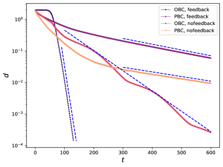
The Fig. S5 shows typical decay behaviors of distances for both Lindbladians with feedback and without feedback under PBCs and OBCs. The different decay behaviors of distances are evident signatures of boundary-sensitive relaxation behaviors.
As shown in Fig. S6, the distances for no-feedback case under OBCs immediately decays as the manner controlled by Liouvillian gap . Therefore, the corresponding relaxation time is given by .