THE BEST CONSTANT FOR INEQUALITY INVOLVING SUM OF THE RECIPROCALS AND PRODUCT OF POSITIVE NUMBERS WITH UNIT SUM
Yagub N. Aliyev
School of IT and Engineering
ADA University
Ahmadbey Aghaoglu str. 61
Baku 1008, Azerbaijan
E-mail: yaliyev@ada.edu.az
Abstract
In the paper we study a special parameter containing algebraic inequality involving sum of reciprocals and product of positive real numbers whose
sum is 1. We determine the best values of the parameter using a new optimization argument. In the case of three numbers the algebraic inequality have some interesting geometric applications involving a
generalization of Euler’s inequality about the ratio of radii of circumscribed
and inscribed circles of a triangle.
††2020 Mathematics Subject Classification: Primary 26D05; Secondary 52A40.††Key words and phrases: best constant, symmetric polynomials, algebraic inequality, geometric inequality, Euler’s inequality.
1 Introduction
Consider the inequality
where , for . Here is a real number and it is asked to find the best (maximal possible) for each . If such exists then we will denote it by .
Note that the right hand side of the inequality (1)
where , is a non-decreasing function of . So if (1) is true for a certain then it is also true for all .
By Cauchy-Schwarz inequality . Since the inequality holds true for , it also holds true for all . So, the best constant , if exists, satisfies .
Case . For the case there is no best constant. If then we obtain the inequality
where . This inequality is true for any . Indeed, if we multiply both sides by , then we obtain
Since , the parameter cancels out, and we obtain
which is always true.
Case . For case the best constant is . We obtain the inequality
where . This inequality is true only for .
We can show this by substituting
, in this inequality. On the other hand we can prove that
holds true. So, is the maximum possible value for this inequality (see [2]). In the solution to problem [2] it was noticed by David B. Leep that the case is equivalent to a more general inequality for symmetric polynomials , , , which can also be writen as
making case almost trivial. Inequality (1) can also be written using symmetric polynomials but as the results for cases and below suggest there is no simple solution for . Let
If , then (1) is equivalent to inequality
homogeneous with respect to variables .
There are some geometric applications of case . The inequality
where and are respectively the circumradius and
inradius, and are sides of a triangle, holds true if . Indeed, substituting , and the corresponding values of
and in (2) we obtain . So, again, if we will prove (2) for then will the best constant for the inequality (2). For we obtain
which is a refinement of Euler’s inequality and follows directly from the case (see [3], [4]).
Another geometric application is the following inequality about the sides of a triangle which follows directly from the case (see [5]):
This inequality can also be written as a quintic inequality of symmetric polynomials
which is a special case () of the following inequality mentioned in [11] (see p. 244, where )
This general inequality is also easily proved if we put , , , and simplfy to obtain
Similar quartic and sextic inequalities were studied in series of works by J.F. Rigby, O. Bottema and J.T. Groenman (see [9], [20] and their references).
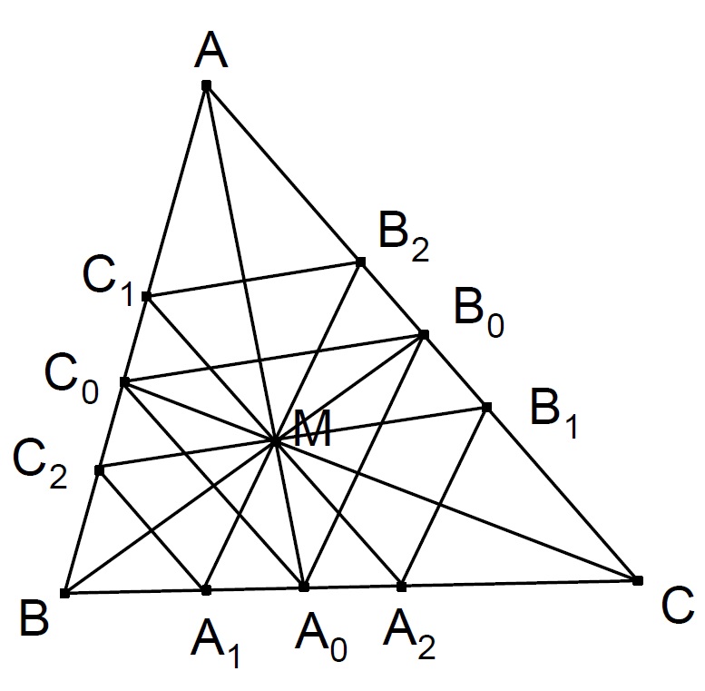
One more geometric application of case is about the areas of triangles and needs introduction of some notations. Let be a point in a triangle . Extend lines , , and to intersect the sides of triangle at , , and , respectively (see Fig. 1). Next construct the parallel to through , which intersects and at and , respectively. Analogously, draw the parallel through to (and to ) to find and (and and ). Denote
where the square brackets stand for the area of the triangles (see [5], [6]). Then
Figure 1: Geometric application of case .
Case . For the case the best constant is (see [3]). In this case we obtain
where . Again this inequality is true only for . Indeed, substituting in this inequality
, , we obtain . On the other hand we can prove that the inequality holds true for .
So, is the maximum possible value for this inequality.
Case . For the case we obtain the inequality
where , and it was conjectured in [3] that the best constant is
where . This conjecture for will be proved in the current paper. Also it will be proved that the equality cases in this inequality occur when and when, for example,
, .
Case . This case was not studied before. Using Maple the exact value of is calculated.
Case is possibly the last case for which these calculations of the exact value are possible.
Case . In view of the fact that quintic and higher order equations are in general not solvable in radicals, it is unlikely that there is a precise formula for the best constant in the cases . Therefore, for the greater values of (), instead of the exact value, it is reasonable to find some bounds or approximations for . In the current paper it is proved that
Some possible improvements for this symmetric double inequality are also discussed.
It is interesting to compare the results of the current paper with the results for the following similar inequality
where The best constant for this inequality is known for all . See Corollary 2.13 in [13] where it is proved that .
In particular, if then we obtain
with equality case possible only when . Inequality (5) also follows from the following inequality for (averages of ),
which holds if and only if
for each (see [13], Theorem 1.1; [10], p. 94, item 77). Indeed, it is sufficient to note that inequality (5) can be written as . This means that the above conditions for () are satisfied as
Since (5) will be essential in the following text, an independent proof of (5) and some generalizations will be given in Appendix. Note also that
Using this and by comparing (1) and (5), we obtain that if , then .
Special cases and of inequality (4) are also of interest for comparison with the corresponding cases of inequality (1). If then the
best constant inequality is
where . Surprisingly, this inequality is also equivalent to a
geometric inequality. One can show that it simplifies to
where is the semiperimeter of a triangle. The last geometric inequality also
follows from the formula for the distance between the
incenter and the centroid of a triangle: (see [3]).
If then the
best constant inequality is
where (see [22], Example 3).
The literature about symmetric polynomial inequalities is extensive [14], [15], [16], [17], [18], [21], [23]. Some of the results of the current paper were presented at Maple Conference 2021 [8].
2 Main Results
Let us consider all cases for in a unified way. Assume first that . Then by using (5), inequality (1) can be written as
where , for . Let us denote the left side of (6) by , which is defined for all points of bounded set
except point . For the points of boundary
function is undefined and, obviously, for each ,
Lemma 1. If , then
Proof. The limit can be interpreted as a single variable limit if we take
where not all constants are equal and . So, we calculate
where we used L’Hôpital’s rule twice and the fact that (Cauchy-Schwarz inequality, the equality case is not possible as not all are equal). Proof is complete.
In particular, if then , and therefore, by Lemma 1,
As an immediate consequence of this and (6), we obtain an upper bound for the best constant
We want to use a well known result
in analysis, which states that a continuous function over a compact set achieves its
minimum (and maximum) values at certain points. For this purpose, let us change function , to new function so that is defined also at point and points of , and is continuous in compact set :
Since is a continuous function in compact , reaches its extreme values somewhere in . Obviously, reaches its maximum value at the boundary points where , and the minimum value at a point of . The minimum of is achieved at the same point of if the minimum point is different from . In any case, . We use an optimization argument similar to [22, 13] but with 3 variables, to determine where these points must lie. This method can also be used for other inequalities involving only symmetric polynomials , , and .
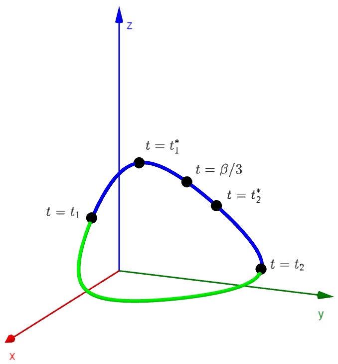
Let be a minimum point of . Select any 3 of the coordinates of , say , , and . Let us assume that and . Since , . Also, by AM-GM inequality and it is known that if then . So, suppose that . Let us now take arbitrary positive numbers such that and . Without loss of generality we can assume that . Since and , the numbers and are the solutions of quadratic equation . If we take then we obtain parametrization of the curve obtained by intersection of plane and surface :
Parameter changes in interval , where and are the zeros of cubic in intervals and , respectively. The third zero of satisfies and therefore . Since we are interested only with case , we will take one half of this curve (see Fig. 2)
and in smaller interval , where and are the zeros of cubic in intervals and , respectively. Again, since the third zero of satisfies , . Note that if , then , and if then . Consider sum and note that
Figure 2: Parametric space curve (blue and green) representing intersection of plane (not shown) and surface (not shown).
Denote , where . So, if , then , and . Consequently, attains its minimum and maximum in interval at endpoints , respectively.
We are interested in making smaller, which happens when sum is smaller. So, the minimum of is reached when . Since the coordinates , , and were chosen arbitrarily, these results hold
for any trio of coordinates. Therefore, the left side of (6) is minimal only when there are at most 2 distinct numbers in the set Furthermore if the two numbers are distinct then the smaller one is repeated times in i.e. . Consequently, in (6) we can restrict ourselves only to the case where , , where . By substituting these in (6) and simplifying, we obtain
We will study the part of the denominator which is dependent on , and for simplicity put . So,
Denote the polynomial in the denominator by
where . By taking the derivative and simplifying, we obtain
Since and , there is at least 1 zero of polynomial in interval . On the other hand, by Descartes’ rule of signs (see p. 247 in [12], or p. 28 in [19]) the number of positive zeros of does not exceed the number of sign changes in the sequence of coefficients of , which is 1. So, has exactly one zero in , which is also maximum point of . This means that there is exactly one point in , such that
, makes the left side of (6) minimal. This minimal value is also the best constant for (1):
For and it is possible to find the exact values of and corresponding .
•
if , then and Therefore, . By (8), the best constant is (see [2]).
•
if , then and Therefore, . By (8), the best constant is (see [3]).
•
if , then and Using Cardano’s formula and Maple, we find that where . By (8), the best constant is
, which coincides with the value of conjectured in [3].
•
if , then
Using Ferrari’s method and Maple, we find that
where
By (8), the best constant is
.
For larger values of , we can give some bounds for . We already found an upper bound (7). We will now focus on a similar lower bound.
By AM-GM inequality,
where , , and . Let us show that if then
where and therefore . Indeed, we can simplify (10) to
where . It is easily proved, as we can write it in the following form
where noting completes proof. From (1), (9), and (10) it follows that if , then (1) holds true. This means that we have now a lower bound for the best constant:
Combining (7) and (11) we obtain the following symmetric double inequality.
Theorem 1. If , then
It is possible to improve these estimates in exchange for less elegant formula. For example, if we put , , then we obtain from (6) a new upper bound for the best constant:
One can check that (13) is sharper than (6) for all . We can also prove that or equivalently, for all . Indeed,
For one can check directly that . For , one can use the fact that and .
3 Appendix
We will give a proof of (5) here. We can use the optimization argument given after Lemma 1 of the current paper, to maximize the left hand side of (5), while keeping the right hand side of (5) fixed. This is achieved when for any 3 of the coordinates, say , , and , of , . So, we can restrict ourselves only to the case where and , where . For this particular case (5) is transformed to
which can be simplified to correct inequality
The equality case is possible only when .
Inequality (5) can also be written as homogeneous inequaity , where and are, respectively, arithmetic, harmonic, and geometric means of arbitrary positive numbers :
Since , automatically for any real number . It would be natural to ask whether general inequality can hold true also for some real number . The answer to this question is negative. A counter example is found if one takes and , where . Indeed, if , then and .
[9]O. Bottema, J.T. Groenman: On some triangle inequalities. Publikacije Elektrotehničkog Fakulteta. Serija Matematika i Fizika, 577/598 (1977), 11–20. http://www.jstor.org/stable/43667788
[10]G. Hardy, J.E. Littlewood And G. Pólya:Inequalities, Cambridge Mathematical Library
2nd ed., 1952.
[11]W.R. Harris:Real Even Symmetric Ternary Forms. Journal of Algebra, 222 (1999), 204–245.
[13]T.P. Mitev:New inequalities between elementary symmetric polynomials. J. Ineq. Pure and Appl. Math.,
4(2) (2003), Article 48.
[14]D. S. Mitrinović:Inequalities Concerning The Elementary Symmetric Functions. Publikacije Elektrotehničkog Fakulteta. Serija Matematika i Fizika, 182 (1967), 17–20.
http://pefmath2.etf.rs/files/71/182.pdf
[15]D. S. Mitrinović:Some Inequalities Involving Elementary Symmetric Functions. Publikacije Elektrotehničkog Fakulteta. Serija Matematika i Fizika, 182 (1967), 21–27.
https://www.jstor.org/stable/43667274
[16]D. S. Mitrinović:Inequalities Concerning The Elementary Symmetric Functions. Publikacije Elektrotehničkog Fakulteta. Serija Matematika i Fizika, 210/228 (1968), 17–19. https://www.jstor.org/stable/43667315
[18]C.P. Niculescu:Interpolating Newton’s Inequalities. Bulletin mathématique de la Société des Sciences Mathématiques de Roumanie, Nouvelle Série, 47(1/2) (95) (2004), 67–83. https://www.jstor.org/stable/43678943
[20]J.F. Rigby:Quartic and sextic inequalities for the sides of triangles, and best possible inequalities. Publikacije Elektrotehničkog Fakulteta. Serija Matematika i Fizika, 602/633 (1978), 195–202. http://www.jstor.org/stable/43660843
[21]S. Rosset:Normalized Symmetric Functions, Newton’s Inequalities, and a New Set of Stronger Inequalities. The American Mathematical Monthly, 96(9) (1989), 815–819. https://www.jstor.org/stable/2324844