W-HMR: Human Mesh Recovery in World Space with Weak-supervised Camera Calibration and Orientation Correction

Abstract

For a long time, in the field of reconstructing 3D human bodies from monocular images, most methods opted to simplify the task by minimizing the influence of the camera. Using a coarse focal length setting results in the reconstructed bodies not aligning well with distorted images. Ignoring camera rotation leads to an unrealistic reconstructed body pose in world space. Consequently, existing methods’ application scenarios are confined to controlled environments. And they struggle to achieve accurate and reasonable reconstruction in world space when confronted with complex and diverse in-the-wild images. To address the above issues, we propose W-HMR, which decouples global body recovery into camera calibration, local body recovery and global body orientation correction. We design the first weak-supervised camera calibration method for body distortion, eliminating dependence on focal length labels and achieving finer mesh-image alignment. We propose a novel orientation correction module to allow the reconstructed human body to remain normal in world space. Decoupling body orientation and body pose enables our model to consider the accuracy in camera coordinate and the reasonableness in world coordinate simultaneously, expanding the range of applications. As a result, W-HMR achieves high-quality reconstruction in dual coordinate systems, particularly in challenging scenes. Codes will be released on project page after publication.

1 Introduction

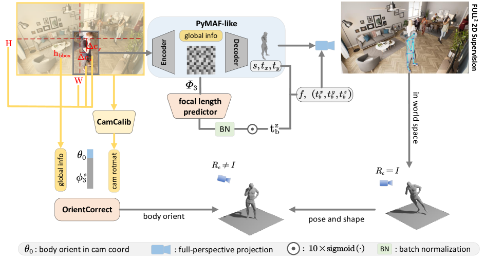
Figure 2: Pipeline of W-HMR. The OrientCorrect takes three vectors as input and outputs body orientation in world coordinate. FULL² 2D supervision refers to 2D joint supervision on full images, which is based on full-perspective camera model. $(\varDelta c_{x},\,\varDelta c_{x})$ are offsets of the bounding box center relative to the center of the original image. Note $\varphi_{3}$ and $\phi_{3}^{s}$ are features. If confused about our feature extraction process, please refer to the supplementary material or [52].

Recovering 3D human meshes from monocular images is a crucial task in human-centered research, with wide-ranging applications in areas such as try-on, animation, and virtual reality. However, there is a noticeable lack of research on global body reconstruction from images captured under complex shooting conditions. The reconstructed bodies outside controlled environments are often unsuitable for real-world applications, as depicted in Fig. 2 and Fig. 5.

Figure 1: Comparison among the camera models used by the other four models [14, 43, 19, 25] and our W-HMR. $f_{crop}$ and $f_{full}$ denote the focal lengths of the full and cropped images, respectively. $R_{c}$ is the camera rotation matrix. The red items mean trainable, i.e., predicted by neural networks.

The primary challenge in this task arises from the limited camera information. Among camera parameters, focal length plays a critical role in distortion effects, influencing the alignment of reconstructed 3D human bodies with original images. Additionally, camera rotation determines the reasonableness of the reconstructed body pose in the world (global) or camera (local) coordinate after coordinate transformation. Fig. 1 illustrates the treatment of the camera in existing models, emphasizing the need for improved methods. The focal length either involves simple manual definitions as seen in HMR [14] and CLIFF [25], or network predictions as utilized by SPEC [19] and Zolly [43]. As for camera rotation, most models [52, 53, 51, 20, 17, 18, 26] do not consider it and recover body in camera coordinate, except for SPEC. Even based on the most comprehensive camera model, SPEC still has limitations due to the inherent flaws in its CamCalib model.

Firstly, the focal length is predicted based on background environmental information, which is inadequate for the body recovery task and cannot handle finer distortions of body parts. To address these challenges, we propose a weak-supervised camera calibration method. The core idea is that we don’t need to predict the original focal length. This method leverages body distortion information to predict a reasonable focal length, eliminating the need for supervision with rare focal length labels and enhancing perspective projection accuracy. Based on the full-perspective camera model, 2D supervision becomes more precise, thereby improving recovery accuracy.

Secondly, the predicted camera rotation is not entirely accurate. With pseudo camera rotation as input, training the model like SPEC to predict poses in world coordinate would lead to error accumulation. The error in pseudo camera parameters would impact the final recovery precision. Consequently, the accuracy of recovery is limited. Additionally, it decreases the model’s generalizability. For example, SPEC’s performance would be worse when the camera rotation is known, as shown in Tab 1. We adopt an indirect approach for predicting body poses in world coordinate. First, we train the model to achieve optimal accuracy of pose and shape in camera coordinate. Then, we propose a novel module named OrientCorrect to assist in correcting body orientation, thus avoiding the issues above.

In summary, we decouple the recovery of the global body into three parts: camera calibration, local body reconstruction, and global body orientation correction. This approach prevents errors in camera parameter prediction from accumulating during model training and inference. Our contribution can be grouped into the following three points:

• We present the first weak-supervised camera calibration method focus on the human recovery task. We achieve reasonable focal length prediction without focal length labels, but relying on human body distortion information. Better mesh-image alignment makes 2D supervision more precise and effectively improves recovery accuracy.

• We design a practical orientation correction module. The module solves the issue that previous methods cannot generate reasonable human poses in world space. This method is simple and effective, and can be well transplanted to other models without destroying the original structure and performance.

• Our decoupling idea successfully mitigates the negative impact of incorrect camera parameter estimation. As a result, our model can achieve remarkable reconstruction results in both coordinate systems simultaneously, which is not possible with past models.

2 Related Work

2.1 Camera Model in Human Recovery

To visualize the reconstruction results and utilize 2D labels, 3D human recovery models require a camera model. The classical HMR [14] employed a weak-perspective camera model, which assumes an extremely large focal length of 5000 pixels to mitigate human distortion. This assumption is suitable for images captured with a long focal length when the human subject is distant from the camera. Due to its simplicity, the weak-perspective camera model has been widely adopted in subsequent works [52, 53, 18, 8, 17].

To the best of our knowledge, Kissos et al. [16] was the first to enhance the weak-perspective camera model in pose estimation. They assumed a constant camera Field of View (FoV) of 55 degrees instead of a fixed focal length. Later, CLIFF [25] also adopted the same camera model. SPEC [19] took a different approach by constructing a new dataset and training a camera parameter prediction model named CamCalib. Zolly [43] predicted the focal length indirectly through a carefully designed translation prediction model, albeit with partial reliance on focal length labels and limitations in focal length prediction for cropped images. Regarding camera rotation, it was usually overlooked in previous works. SPEC was the pioneering work to advocate for the recovery of the body in world coordinate for postural plausibility. It relied on CamCalib to predict camera parameters and used these parameters as model inputs to directly predict the global body. However, its one-step approach led to error accumulation, constraining reconstruction accuracy and application scope. In contrast, our decoupling of this process effectively addresses these issues.

2.2 Regression-based Method

In the domain of 3D human body reconstruction, methods can be broadly classified into regression-based and optimization-based approaches. Optimization-based methods are beyond the scope of this paper and can be explored in the literature review [40]. Regression-based models can be further categorized into model-based and model-free approaches based on the output type. Model-based models refer to those that output template parameters, with the majority of current models [14, 8, 52, 17, 18] still relying on the SMPL algorithm [29], and a few [37, 57, 49, 50] based on SCAPE [2], GHUM&GHUML [46], and SMPL-X [36]. These models leveraged the prior knowledge embedded in parameter models but were limited to reconstructing finer mesh details due to constraints in degrees of freedom.

In contrast, model-free models in this field output voxels [41, 56], UV position maps [54, 39] and 3D vertex coordinates [26, 33, 27, 5]. Here, we mainly focus on methods that output 3D vertex coordinates. Apart from methods that output voxels, all other output types would be converted to 3D vertices and then transformed into meshes based on predefined triangle faces. One classic model-free method, Graphormer [26], designed a regression module based on transformer[6], which directly outputs 431 3D sparse vertices. The advantage of model-free models is that they can recover more details than model-based models. However, their limitations lie in their inability to effectively utilize prior knowledge of the human body, and their models tend to have larger sizes. To overcome the limitations of both model-based and model-free approaches, we propose a hybrid method where the model-based regression module provides a strong initialization, and the model-free module further refines the results. This approach aims to achieve optimal mesh precision with relatively fewer parameters, bridging the gap between model-based and model-free methods.

3 Method

3.1 Preliminary

Perspective Camera Model In the perspective camera model, camera parameters are divided into intrinsic and extrinsic parameters. The intrinsic parameters $K\in\mathbb{R}^{3\times 3}$ are generally represented by a matrix as follows

$$K=\left[\begin{matrix}f_{x}&0&c_{x}\\ 0&f_{y}&c_{y}\\ 0&0&1\\ \end{matrix}\right]$$ (1)

Here, $f_{x}$ and $f_{y}$ represent the focal lengths in the x-axis and y-axis directions, respectively. $(c_{x},\,c_{y})$ is the principal point coordinate. Considering common situations, researchers often assume $f_{x}=f_{y}$ and $(c_{x},\,c_{y})$ in the center of the image. The extrinsic parameters include a camera rotation matrix $R_{c}\in\mathbb{R}^{3\times 3}$ and a camera translation vector $t_{c}\in\mathbb{R}^{3}$. For most methods based on camera coordinate, they generally assume $R_{c}=I$ and $t_{c}=(0,\,0,\,0)$. Therefore, we can get $R_{b}=R_{c}^{-1}R_{b}^{c}=R_{b}^{c}$, where $R_{b}$ is the body orientation in world coordinate (global orientation) and $R_{b}^{c}$ is the body orientation in camera coordinate (local orientation). This is why conventional models often produce unrealistic human body poses in the real world when dealing with images without known camera parameters.

When we have a 3D point $p=(X,\,Y,\,Z)$ (3D joint or mesh vertex) and want to project it onto the imaging plane to get a 2D point $p=(x,\,y,\,z)$, we calculate following the formula $p^{T}=K(p+t_{b})^{T}$, where $t_{b}=(t_{b}^{x},\,t_{b}^{y},\,t_{b}^{z})$ represents the translation of the body relative to the camera. The projection point $p$ is converted into a perspective projection point $p_{p}=(x_{p},\,y_{p})$ according to

$$\left[\begin{array}[]{c}x_{p}\\ y_{p}\\ \end{array}\right]=\left[\begin{array}[]{c}\frac{x}{z}\\ \frac{y}{z}\\ \end{array}\right]=\left[\begin{array}[]{c}\frac{fX+c_{x}\left(Z+t_{b}^{x}\right)}{Z+t_{b}^{z}}\\ \frac{fY+c_{y}\left(Z+t_{b}^{y}\right)}{Z+t_{b}^{z}}\\ \end{array}\right]$$ (2)

The whole process is how a 3D object is imaged on a 2D plane based on the perspective camera model. You may notice from Equ. 2 that when $f$ is set very large, the effect of $Z$ would become negligible and the perspective effect disappears. The consequence is that the human mesh does not align well with the original image, making 2D supervision in error and ultimately affecting recovery accuracy.

Translation and Scale Following  [14], we continue to utilize SMPL parameters $\varTheta$ as our template. The SMPL parameters encompass pose $\boldsymbol{\theta}\in\mathbb{R}^{24\times 3}$, shape $\boldsymbol{\beta}\in\mathbb{R}^{10}$, where $\boldsymbol{\theta}_{0}$ is the body orientation. Specifically, pose $\boldsymbol{\theta}$ and shape $\boldsymbol{\beta}$ can be inputted into a pre-defined function $M\left(\boldsymbol{\theta},\boldsymbol{\beta}\right)\in\mathbb{R}^{3\times N}$ to obtain $N$ vertex coordinates, i.e., $(X,Y,Z)$ we talk about before. The mesh derived from these vertices is the reconstructed human mesh. To project it onto the image, the model outputs three additional parameters, i.e., translation $(t_{x},t_{y})$, and scale $\boldsymbol{s}$. As for $\boldsymbol{s}$ and $(t_{x},t_{y})$, they serve to determine the size and position of the human meshes within the cropped image. Based on the usual assumptions, we assume a human body range of 2 meters, which establishes the relationship between $t_{b}^{z}$ and $f$ as

$$\frac{t_{b}^{z}}{2}=\frac{f}{sh_{bbox}}$$ (3)

where $h_{bbox}$ refers to the height of the bounding box. For a more detailed reasoning process, please refer to [25] or [16]. Our goal is to leverage the relationship between $t_{b}^{z}$ and $f$ to indirectly predict $f$ by getting $t_{b}^{z}$, thus achieving full perspective.

3.2 Weak-supervised Camera Calibration

Focal length prediction is essentially an ill-posed problem. From Sec. 3.1, we can see that there are too many influencing factors in the process from 3D objects to 2D images. Trying to predict the true focal length through a neural network is almost impossible. So, we propose to use the human body distortion information to predict a ”reasonable” focal length for full-perspective projection.

Camera Calibration The focal length predictor takes the final feature map $\varPhi_{3}$ as input and output a single value $t_{b}^{z}$. To constrain the range of the predicted $t_{b}^{z}$ [43], we employ a sigmoid function and scale it by 10. This adjustment is necessary because distortion becomes irrelevant when a person stands 10 meters from the camera. We add batch normalization to avoid gradient vanishing or exploding caused by the sigmoid function. The focal length can be calculated according to $f=\frac{2sh_{bbox}t_{b}^{z}}{2}$, where the height of bounding box $h_{bbox}$ is known and scale $s$ is output by the PyMAF-like regression module. From Equ. 2, to implement the projection, we also need to know the translation of the body to the camera. $t_{b}^{z}$ has already been generated, so we need to further compute $(t_{b}^{x},t_{b}^{y})$. Following [16], $(t_{b}^{x},t_{b}^{y})=(t_{x},t_{y})$ when projecting in cropped image. But in the full image, the conversion functions for $(t_{x},t_{y})$ to $(t_{x}^{b},t_{y}^{b})$ are summarized below

$$\left[\begin{array}[]{c}t_{b}^{x}\\ t_{b}^{y}\\ \end{array}\right]=\left[\begin{array}[]{c}t_{x}\\ t_{y}\\ \end{array}\right]+{{\left(2\left[\begin{array}[]{c}c^{x}_{bbox}\\ c^{y}_{bbox}\\ \end{array}\right]-\left[\begin{array}[]{c}W\\ H\\ \end{array}\right]\right)}\Bigg{/}{sh_{bbox}}}$$ (4)

where $(c^{x}_{bbox},\,c^{y}_{bbox})$ is the center of the bounding box and $(W,H)$ is the width and height of the full image. The reason why projection is important in the human recovery task is that we need to use rich 2D joint labels to enhance supervision and improve model performance.

Weak Supervision Our main losses can be categorized into three kinds: joint loss, vertex loss, and parameter loss. In this section, we only introduce the joint loss. Please refer to the supplementary material for information on the others. The joint loss can be calculated using the following function:

$$\begin{split}\mathcal{L}_{joint}&=\lambda_{1}MSE\left(J_{3D},\hat{J}_{3D}\right)\\ &+\lambda_{2}MSE\left(J_{2D},\hat{J}_{2D}\right)\\ &+\lambda_{3}MSE\left(J_{2D}^{full},\hat{J}_{2D}^{full}\right)\cdot\left(\frac{W}{w_{bbox}},\frac{H}{h_{bbox}}\right)\end{split}$$ (5)

where $MSE(\cdot)$ represents mean square error. The $J_{3D}$ denotes 3D joints, which are regressed from mesh vertices[14]. $J_{2D}$ signifies normalized 2D joint coordinate in the cropped image and ${J}_{2D}^{full}$ is normalized 2D joint coordinate in the full image. Note that 2D joints are the projected 3D joints on images. The last term in the Equ. 5 is the key of our FULL² 2D supervision. It is worth mentioning that $\left(\frac{W}{w_{bbox}},\frac{H}{h_{bbox}}\right)$ is used to dynamically balance the weights and prevent the FULL² 2D loss from being too small, which could lead to ineffective supervision.

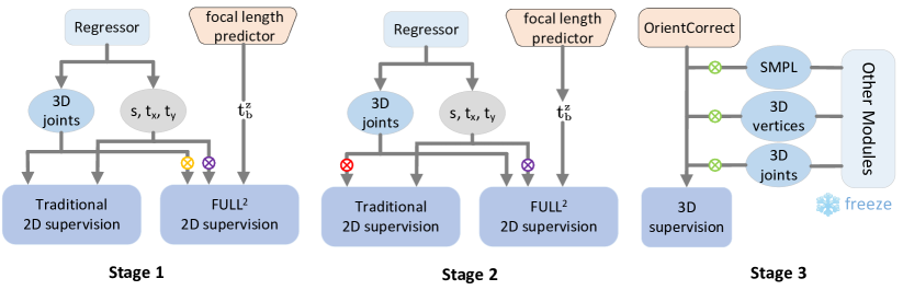
Figure 3: This figure depicts our model training paradigm, illustrating the detachment strategy at different stages to achieve stable model training. The colorful symbol $\otimes$ represents detachment. Traditional 2D supervision refers to projecting 3D joints onto the cropped image to get 2D joints based on the weak-perspective camera model, just as traditional models would do.

Weak supervision is reflected in this FULL² 2D supervision. We do not use any real focal length label to supervise the training of the focal length predictor. From Sec 3.1, we know that the focal length is involved in the 3D to 2D projection. So in having 2D and 3D joint labels, we can let the predictor learn how to generate a correct focal length for 3D to 2D joint projection. After all, all this effort to make the projection more precise is for that the model can be trained more accurately. The purpose determines the method. By the way, rich joint labels are clearly easier to collect for model training than rare focal length labels.

3.3 Orientation Correction

Our goal is to recover human mesh in world space. Weak-supervised camera calibration can only help the model to get the optimal mesh accuracy in camera coordinate. After that, we need to consider how to keep the human pose reasonable in world coordinate without destroying the original accuracy. In short, we need to predict the body orientation in world coordinate to replace the body orientation generated in camera coordinate.

We propose the OrientCorrect for predicting body orientation in world coordinate. This module’s input comprises the camera rotation $R_{c}$ predicted by CamCalib, spatial body features $\phi_{3}^{s}$, global information, and the body orientation $\theta_{0}$ in camera coordinate. The $\theta_{0}$ is predicted by the PyMAF-like module. The output of OrientCorrect is the human body orientation in world coordinate. The specific procedure can be expressed as follows:

$$R_{b}=R_{b}^{c}+FC\left(\oplus\left(\phi_{i}^{s},\,\,glob\_info,R_{c},R_{b}^{c}\right)\right)$$ (6)

where $\oplus$ represents concatenation, $FC(\cdot)$ are couples of FC layers. The global information $glob\_info=\left\{\frac{\varDelta c_{x}}{\tilde{f}},\frac{\varDelta c_{y}}{\tilde{f}},\frac{h_{bbox}}{\tilde{f}},\frac{W}{\tilde{f}},\frac{H}{\tilde{f}}\,\,\right\}$ and it is important auxiliary information for predicting body orientation [25]. As for $\tilde{f}$, it is for normalization and $\tilde{f}=\sqrt{W^{2}+H^{2}}$. This iterative approach is employed to obtain the final body orientation in world coordinate. The OrientCorrect is a completely separate module. But it not only makes full use of what the model has learnt in camera coordinate, but also avoids destroying the body feature space that the model has constructed. Additionally, this method can be easily applied to other models based on camera coordinate without reducing the original precision.

Model	AGORA				HUMMAN			SPEC-MTP
	NMVE$\downarrow$	NMJE$\downarrow$	MVE$\downarrow$	MPJPE$\downarrow$	MPJPE$\downarrow$	PA-MPJPE$\downarrow$	PVE$\downarrow$	MPJPE$\downarrow$	PA-MPJPE$\downarrow$	PVE$\downarrow$
HMR [14]	217.0	226.0	173.6	180.5	43.6	30.2	52.6	121.4	73.9	145.6
HMR-f [14]	-	-	-	-	43.6	29.9	53.4	123.2	72.7	145.1
SPEC [19]	126.8	133.7	106.5	112.3	44.0	31.4	54.2	125.5	76.0	144.6
CLIFF [25]	83.5	89.0	76.0	81.0	42.4	28.6	50.2	115.0	74.3	132.4
PARE [18]	167.7	174.0	140.9	146.2	53.2	32.6	65.5	121.6	74.2	143.6
GraphCMR [21]	-	-	-	-	40.6	29.5	48.4	121.4	76.1	141.6
FastMETRO [4]	-	-	-	-	38.8	26.3	45.5	123.1	75.0	137.0
PLIKS [39]	71.6	76.1	67.3	71.5	-	-	-	-	-	-
ProPose [7]	78.8	82.7	70.9	74.4	-	-	-	-	-	-
HybrIK [23]	81.2	84.6	73.9	77.0	-	-	-	-	-	-
Hand4Whole [34]	90.2	95.5	84.8	89.8	-	-	-	-	-	-
PyMAF [52]	87.3	92.6	78.6	83.3	42.5	28.9	50.4	108.6	66.1	127.5
Ours∗	78.1	87.0	70.3	78.3	37.4	29.1	40.5	104.5	61.7	118.7
Ours†	68.7	77.7	61.8	69.9	39.2	30.8	40.4	104.9	62.3	115.2
Ours-P†	70.4	75.4	63.4	67.9	36.5	27.1	43.5	108.1	65.7	121.5

Table 1: Comparison with SOTA methods on distorted datasets in camera coordinate. Some of the evaluation results on HuMMan [3] and SPEC-MTP [19] are sourced from  [43], while the evaluation results on AGORA [35] are obtained from its official website https://agora-evaluation.is.tuebingen.mpg.de/. Including the following tables, ^∗ represents backbone is ResNet50 [11], ^† means VitPose-B [47, 48], and ”P” denotes the pure parameter module. Note we do not perform any fine-tuning on SPEC-MTP. The baseline structure is kept the same as [52], but its training dataset and evaluation settings are the same as ours.

3.4 Training Paradigm

In the first stage, after obtaining the 3D joints, we need to project them onto both the cropped image and the original image to obtain $J_{2D}$ and $J_{2D}^{full}$, respectively. $J_{2D}$ still adheres to the traditional weak-perspective camera model, while $J_{2D}^{full}$ uses the full-perspective camera model. During the FULL² 2D supervision, we detach the gradients of the 3D joints, scale $s$, and translation $(t_{x},\,t_{y})$ to prevent incorrect backpropagation. This precaution is necessary because, in the first stage, the focal length predictor cannot predict a reasonable focal length. This would lead to a completely erroneous 2D joint loss, affecting the regressors to learn to reconstruct the human body. To stabilize the training of the focal length predictor, we introduce an additional loss in the first stage, i.e.,

$$\mathcal{L}_{f}=MSE\left(f,\tilde{f}\right)$$ (7)

where $\tilde{f}=\sqrt{W^{2}+H^{2}}$ serves as pseudo focal length labels to ensure focal length predictor outputs coarse but relatively reasonable results. Note it is only applied in stage 1.

Since the model has already developed initial capabilities in predicting joint points and focal lengths in the first stage, we can directly apply FULL² 2D supervision without concern about training collapse. We continue to detach $(s,\,t_{x},\,t_{y})$ from the full-perspective projection. Because the perspective effect does not impact the model’s learning of scale and translation. In the second stage, we detach the gradients of the 3D joints from the weak-perspective projection to prevent erroneous backpropagation of the weak-perspective 2D joint loss on cropped images.

In the first two stages, training is conducted entirely in camera coordinate. In the third stage, we need to equip the model to reconstruct the human body in world coordinate. The pre-trained regressors, focal length predictor, feature extractor, and CamCalib are frozen at this stage. We only need to train the OrientCorrect composed of three FC layers. We exclusively use the 3D joint, mesh vertices, and SMPL parameters in world coordinate for supervision.

4 Experiment

4.1 Implement Details

We train three models based on [52] for evaluation. Two of them utilize a hybrid regression module, using 431 sparse vertices for downsampling. The distinction lies in using different backbones, including ResNet50 [11] and VitPose-B [47]. Additionally, we train an extra model using a pure parameter regression module, employing 67 mocap markers for downsampling, with the backbone being VitPose-B. For training, we utilize datasets such as Human 3.6m [12], 3DPW [42], MPII3D [31], MPII [1], AGORA [35], COCO [28], SPEC-SYN [19], and HuMMan [3]. Some of the datasets are augmented with pseudo-labels generated by CamCalib, EFT [13], or CLIFF [25]. Please refer to the supplementary materials for detailed structural variations and training settings of our different models. Our model can simultaneously provide results in camera and world coordinate. But if results in world coordinate are not needed or camera rotation is known, the CamCalib and OrientCorrect can be discarded. The focal length predictor can also be discarded if mesh projection is not required.

4.2 Evaluation Results

We conduct evaluations on multiple benchmarks. Our model’s performance presentation is divided into camera and world coordinates in the main text. Our model is also evaluated on conventional benchmarks such as 3DPW [42] and h36m [12], yielding outstanding results too. Supplementary materials are available for further reference. Below are the main results and analysis.

Model	SPEC-MTP
	W-MPJPE$\downarrow$	PA-MPJPE$\downarrow$	W-PVE$\downarrow$
GraphCMR [21]	175.1/166.1	94.3	205.5/197.3
SPIN [20]	143.8/143.6	79.1	165.2/165.3
PartialHumans [38]	158.9/157.6	98.7	190.1/188.9
I2L-MeshNet [33]	167.2/167.0	99.2	199.0/198.1
HMR [14]	145.2/128.8	71.8	164.6/150.7
PyMAF [52]	148.8/134.2	66.7	166.7/158.7
Ours-P†	139.3/130.3	66.6	155.8/147.8
SPEC[19]	124.3	71.8	147.1
Ours-P†	118.7	66.6	133.9

Table 2: Comparison with SOTA methods on SPEC-MTP [19]. The first six models in the table are all methods that output results in camera coordinate, so there are two results. The ”a” in ”a/b” indicates the result calculated directly using the output in the camera coordinate. The ”b” is the result calculated after the output has been calibrated by camera rotation predicted by CamCalib. The latter two models can directly get the results in world coordinate without calibration, so there is only one result.

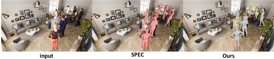
Figure 4: Qualitative results on AGORA compared with SPEC [19]. The areas marked within the red circles indicate the mismatch between the SPEC reconstructed mesh and the original image. In contrast, by comparing it with the corresponding W-HMR reconstructed results enclosed in the yellow circles, it is evident that our approach exhibits stronger capabilities in handling complex samples.

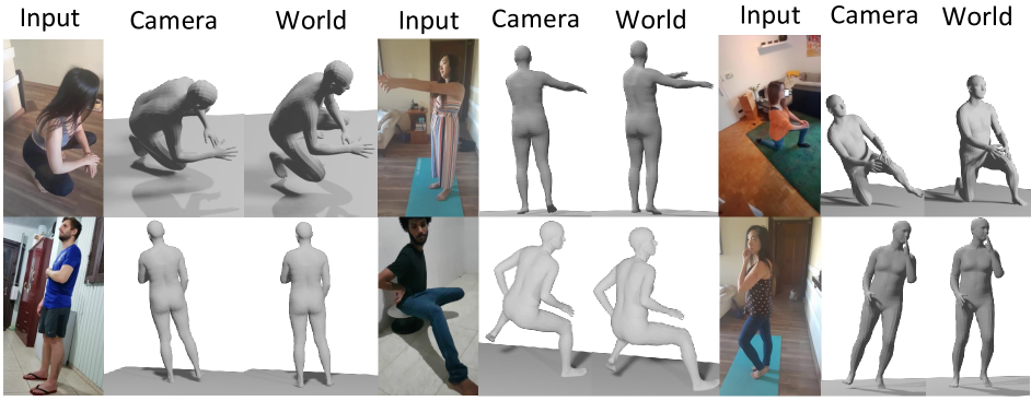
Figure 5: Qualitative results on SPEC-MTP [19]. ”Input” refers to input images. ”Camera” represents the output in the camera coordinate. ”World” represents the output in world coordinate.

Camera Coordinate In our study, we choose three challenging datasets containing distorted images to showcase the superiority of weak-supervised camera calibration under complex conditions. As depicted in Tab. 1, our method surpasses the performance of most existing methods on the challenging synthetic dataset AGORA [35]. Each of our models demonstrates unique strengths. The pure regression model achieves higher accuracy in joint localization, and the hybrid regression module excels in capturing mesh details. Compared to baseline [52], our improvement is quite substantial. As depicted in Fig. 4, the W-HMR outperforms SPEC [19] in handling occlusions, rare body rotations, and body intersections. Although the joint accuracy does not exhibit significant improvement on the indoor dataset HuMMan [3], we achieve an 11% improvement in PVE, even surpassing the model-free method FastMETRO [4]. The most remarkable performance is observed on the real distorted dataset SPEC-MTP. We significantly elevate the SOTA results on SPEC-MTP to new heights.

World Coordinate We utilize SPEC-MTP [19] as the primary evaluation dataset. Due to its only test set, specific fine-tuning is not feasible. It adopts a shooting method different from traditional datasets, resulting in unique rotation and severe distortion. Therefore, it poses a significant challenge and is particularly suitable for demonstrating OrientCorrect’s strength. To ensure fairness, we only evaluate the W-HMR with a pure parameter regression module. W-HMR easily outperforms existing methods, including SPEC. It is important to note that W-HMR does not rely solely on higher reconstruction accuracy. Upon comparing our results calibrated by CamCalib with those corrected by OrientCorrect, it is evident that our module is effectively functioning. As illustrated in Fig. 5, the reconstructed human body pose appears implausible in world space when the camera coordinate is not aligned with the world coordinate. However, our OrientCorrect effectively corrects the orientation of the human body and maintains its reasonableness in world coordinate. Our model can accurately perceive and correct both slight and significant camera rotation. Quantitative and qualitative results both demonstrate that our method is simpler and more efficient than SPEC, which will be further substantiated in subsequent ablation study.

4.3 Ablation Study

Our ablation study is primarily divided into two parts. The first part focuses on ablating our model’s camera calibration to demonstrate our approach’s effectiveness in enhancing reconstruction accuracy. Specifically, the main idea is to verify the validity of the global information for the camera calibration. The second part involves ablating different global orientation recovery methods. We will show the limitations of previous methods and demonstrate the robustness of W-HMR. Please refer to supplementary materials for more ablation study.

			AGORA
V	F	G	NMVE$\downarrow$	NMJE$\downarrow$	MVE$\downarrow$	MPJPE$\downarrow$
[HTML]EFEFEF			87.3	92.6	78.6	83.3
$\surd$			82.4	88.6	75.8	81.5
[HTML]EFEFEF $\surd$	$\surd$		81.2	89.3	74.7	82.2
$\surd$		$\surd$	80.7	87.7	73.4	79.8
$\surd$	$\surd$	$\surd$	79.8	87.6	72.6	79.7

Table 3: The ablation study on the core block of the W-HMR. The experiments above utilize ResNet50 [11] as the backbone. In this table, ”V” refers to the vertex regressor. ”F” indicates whether the focal length predictor and FULL² 2D supervision are implemented. ”G” signifies the addition of global information during input.

Camera Calibration We select PyMAF[52] as our baseline and consistently use ResNet50 as the backbone throughout our ablation study, with 431 sparse vertices as the downsampling points. The training and evaluation settings are all kept the same. From the Tab 3, it is evident that the most significant improvements stem from the addition of the vertex regressor and global information. The inclusion of the vertex regressor enhances the model’s ability to reconstruct body mesh details accurately. But, global information not only contributes independently but also aids in the functioning of camera calibration. A comparison between ”V” and ”V+F” reveals that solely adding the focal length predictor only has a noticeable impact on vertex accuracy. However, comparing ”V+G” and ”V+F+G” demonstrates that the presence of global information leads to more substantial improvements when combined with the focal length predictor. This finding further supports our idea that global information is crucial not only for recovering body orientation but also for predicting focal lengths and correcting distortions. In summary, with the camera calibration assistance, W-HMR achieves a decent reconstruction accuracy, which provides a solid foundation for human body recovery in world space.

Model	SPEC-SYN
	W-MPJPE$\downarrow$	PA-MPJPE$\downarrow$	W-PVE$\downarrow$
GraphCMR [21]	181.7/181.5	86.6	219.8/218.3
SPIN [20]	165.8/161.4	79.5	194.1/188.0
PartialHumans [38]	169.3/174.1	88.2	207.6/210.4
I2L-MeshNet [33]	169.8/163.3	82.0	203.2/195.9
HMR [14]	128.7/96.4	55.9	144.2/111.8
PyMAF [52]	126.8/88.0	48.7	136.7/118.0
Ours-P†	127.8/106.2	46.2	137.8/132.6
SPEC [19]	74.9(124.3)	54.5(71.8)	90.5(147.1)
Ours-P†(spec-like)	68.2(185.0)	43.6(63.3)	76.4(208.7)
Ours-P†	82.1(118.7)	46.1(66.6)	93.3(133.9)

Table 4: The ablation study on body orientation correction. ”spec-like” refers to using a similar method like SPEC to predict global pose directly. The numbers in brackets are the evaluation results on SPEC-MTP. This is the reason why we don’t choose the spec-like method. Its impressive results are based on overfitting and sacrificing generalization.

Orientation Correction We select two methods for evaluation. The first method is similar to SPEC. SPEC concatenates features and the camera parameters obtained from CamCalib, then inputs them into a regressor to directly recover the human body in world coordinate. As demonstrated in Tab. 4, the spec-like method significantly outperforms previous methods. However, we attribute this performance to overfitting. The model relies on massive parameters to memorize the global body orientation in the training set of SPEC-SYN, subsequently achieving excellent results on the test set. This is supported by the inferior performance of spec-like methods, such as results on SPEC-MTP. This indicates the susceptibility of such methods to overfitting, potentially leading to the misconception that the model has captured environmental information. What’s worse is that this design destroys the model’s original learned knowledge, making the overall reconstruction less precise. In contrast, our method offers a simpler structure, requires less training data, and exhibits greater robustness. Furthermore, other models based on camera coordinate can easily adopt our approach to achieve global pose recovery.

5 Conclusion

We proposed the first model capable of reconstructing human bodies accurately and reasonably in both camera and world coordinates. To achieve this, we designed a weak-supervised camera calibration method. Our model can generate appropriate focal lengths based on body distortion information, eliminating the dependence on background information and focal length labels. Additionally, we introduced a new orientation correction module that is simpler and more robust compared to previous methods. With a carefully designed training paradigm and model framework, we achieved SOTA performance across multiple datasets in both coordinates. We hope that our work will contribute to the study of human mesh recovery in world space.

Supplementary Material

6 About Datasets

In our experiments, we utilize the following datasets: Human 3.6M [12], 3DPW [42], MPII [1], COCO [28], MPI-INF-3D [31], AVA  [9], AIC [45], Insta [15], AGORA [35], SPEC-SYN [19], SPEC-MTP [19], and HuMMan [3]. To evaluate our model, we conduct experiments on the distorted datasets AGORA, HuMMan, and SPEC-MTP. Furthermore, following traditional practices[44, 52], we also evaluate our model on 3DPW, Human 3.6M, and MPII-INF-3D. For the ablation experiments, we employ AGORA’s evaluation platform as a standard due to its diverse scenes, characters, and shooting methods. We believe that the evaluation results obtained on AGORA are more representative. For human recovery in world space, We additionally perform ablation study on SPEC-SYN to validate the robustness of our method. Following are details about each dataset.

3DPW’ [42] full name is ”3D Human in the Wild.” It is an outdoor dataset that captures actor information using motion capture devices. This dataset is known for its difficulty and has been widely used by researchers to demonstrate the robustness of their methods. Following past conventions, we train two models, one without 3DPW for training and another using 3DPW for training, to evaluate our model’s performance.

Human 3.6M [12] is widely used as the standard dataset to assess the estimation of 3D human pose and the recovery of human mesh. To reduce data redundancy, the original videos are down-sampled from 50 to 10 fps, resulting in 312,188 frames available for training and 26859 frames for evaluation. Following established protocols, we utilize five subjects (S1, S5, S6, S7, S8) for training and two subjects (S9, S11) for evaluation.

MPII [1] is collected from YouTube and comprises a diverse range of activities in various scenes. Based on [53, 8], we only utilize the portion with pseudo 3D labels, which contains approximately 14,000 images.

COCO [28] is a large-scale image dataset widely used for various computer vision tasks such as object detection, image segmentation, and image classification. For our task, we primarily utilize the part including human subjects. COCO provides 2D joint location labels. Based on this, we use corresponding pseudo 3D labels generated by [25, 13, 22], following [53, 25, 8].

MPI-INF-3D [31, 32] is a large-scale 3D dataset that includes both indoor and outdoor scenes. To reduce data redundancy, we extract every 10th frame. The dataset is divided into a training set and a test set according to their original partitioning. The training set comprises 96,507 images, while the test set contains 2929 images. We use pseudo SMPL parameter labels generated by [13].

AVA [9], AI Challenger[45] and InstaVariety [15] are three huge wild datasets that lack real 3D labels. However, in the Human4D [8], researchers utilized VitPose [47] to obtain 2D keypoints and VitDet [24] to generate bounding boxes for human targets. Based on these 2D pseudo labels, they employed ProHMR [22] to acquire pseudo SMPL labels. Subsequently, we further optimize these pseudo-labeled datasets by selecting higher-quality samples for training our model.

AGORA [35] is a multi-person synthetic dataset that has gained recognition in recent years due to its precise SMPL-X labels, complex characters and scenes, and fair evaluation methods. The dataset is available in two resolutions: 1280x720 and 3840x2160. We exclusively utilize the low-resolution set in our work. The train, validation, and test sets are used according to their original partitioning. The bounding boxes used in the test set are obtained using the 2D keypoints generated by Hand4Whole [34].

SPEC-SYN and SPEC-MTP are datasets proposed in SPEC [19]. Inspired by AGORA, SPEC-SYN is also a synthetic dataset with 3,783 images synthesized from five large-scale virtual scenes. It offers a relatively high diversity of focal lengths. On the other hand, SPEC-MTP is a real dataset with SMPL-X labels generated by multi-view fitting. It consists of 3,284 images, which we solely use for evaluating our model. The dataset is challenging because of its serious distortion and special shooting angle.

HuMMan[3] is a high-precision human dataset constructed indoors. It includes labels such as keypoints, point clouds, meshes, SMPL parameters, textures, and more. We only utilize its SMPL labels. We sample every five images to form a training set comprising approximately 84,000 images. Due to the short focal length during data collection, it contains a significant amount of distorted data. Therefore, we also use HuMMan as one of our evaluation datasets. The partitioning of the train and test sets follows the original division provided by the dataset creators.

	ResNet50+vertices	ResNet50+markers	VitPose-B+vertices	VitPose-B+markers
[HTML]EFEFEF $H_{c}\times W_{c}$	224$\times$224	224$\times$224	256$\times$192	256$\times$192
$\{H_{i}\times W_{i}\}_{i=1}^{3}$	{14$\times$14,28$\times$28,56$\times$56}	{14$\times$14,28$\times$28,56$\times$56}	{32$\times$24,64$\times$48,128$\times$96}	{32$\times$24,64$\times$48,128$\times$96}
[HTML]EFEFEF $C_{i}^{fc}$	5	32	5	32
$H_{g}\times W_{g}$	21$\times$21	8$\times$8	24$\times$18	9$\times$7
[HTML]EFEFEF $\{C_{i}^{s}\}_{i=1}^{3}$	{2205,2155,2155}	{2048,2144,2144}	{2160,2155,2155}	{2016,2144,2144}

Table 5: This table illustrates the changes in the size of input images and features when using different backbones (ResNet50 or VitPose-B) and employing different downsampling methods (sparse vertices or markers). As for the symbols, please refer to Sec 8.1.

7 Other Losses

Since we employ a hybrid regression module, we obtain 431 sparse vertices, 1723 coarse vertices, and 6840 complete vertices from the vertex regressor. Therefore, we design a triple vertex loss function, denoted as

$$\begin{split}\mathcal{L}_{vertex}&=\lambda_{4}L1\left(V_{sparse},\hat{V}_{sparse}\right)\\ &+\lambda_{5}L1\left(V_{coarse},\hat{V}_{coarse}\right)\\ &+\lambda_{6}L1\left(V_{complete},\hat{V}_{complete}\right)\end{split}$$ (8)

where $L1(\cdot)$ is L1 loss. We also directly supervise the obtained SMPL parameters by calculating the function as

$$\mathcal{L}_{SMPL}=\lambda_{7}MSE\left(\beta,\hat{\beta}\right)+\lambda_{8}MSE\left(\theta,\hat{\theta}\right)$$ (9)

where $\beta$ is shape parameters in SMPL and $\theta$ is pose parameters which is represented as 9D rotation matrix.

To enhance the model’s ability to focus on human regions and extract refined body information, we include two additional sub-tasks for auxiliary supervision inspired by [52].

First, let’s delve into the IUV map, which is integral to the IUV loss. The IUV map, as defined in [10], uses ”I” to indicate the body part to which a pixel belongs and ”UV” to represent the 2D coordinates on the surface of the body part. This mapping establishes dense correspondences from 3D mesh to 2D plane. We employ three 2D convolution layers to predict the IUV map based on the feature map $\varPhi_{3}$ and render the ground truth online. The loss function is defined as

$$\begin{split}\mathcal{L}_{IUV}&=\lambda_{9}CrossEntropy\left(P,\hat{P}\right)\\ &+\lambda_{10}SmoothL1\left(\hat{P}\odot U,\hat{P}\odot\hat{U}\right)\\ &+\lambda_{11}SmoothL1\left(\hat{P}\odot V,\hat{P}\odot\hat{V}\right)\end{split}$$ (10)

where $\odot$ means masking, which indicates only the foreground pixels are applied. The IUV loss focuses solely on supervising the 2D information, neglecting the depth information, which is essential for capturing distorted details. To address this limitation, we introduce an additional depth map loss. We generate ground truth depth maps by rendering online. A 2D convolution is used to predict the depth map based on the feature map $\varPhi_{3}$. The loss is computed as follows:

$$\mathcal{L}_{depth}=\lambda_{12}L1_{smooth}\left(\frac{1}{D},\frac{1}{\hat{D}}\right)$$ (11)

where we use the reciprocal of the depth for normalization.

8 Implement Details

8.1 Pixel-aligned Feature Extractor

We follow the feature extraction method of [52] but use different sampling points and backbones. When a cropped image $I\in\mathbb{R}^{H_{c}\times W_{c}}$ is inputted into the encoder, it generates an initial feature map $\varPhi_{0}\in\mathbb{R}^{C\times H_{0}\times W_{0}}$. Subsequently, this feature map $\varPhi_{0}$ undergoes further processing through a series of deconvolution layers to yield high-resolution features $\left\{\varPhi_{i}\in\mathbb{R}^{C_{i}\times H_{i}\times W_{i}}\right\}_{i=1}^{3}$. For the first high-resolution feature map $\varPhi_{1}$, a $H_{g}\times W_{g}$ grid is defined to sample finer point-wise features. However, for the second and third feature maps, we project vertices of the mesh obtained from the previous step onto the feature map to sample point-wise features. In summary, we extract spatial features based on the following formula.

$$\phi_{i}^{s}=\oplus\left(fc\left(bs\left(\varPhi_{i},P_{i-1}\right)\right)\right),\,i\in\{1,\,2,\,3\}$$ (12)

where $P_{i}$ represents the projected 2D point for sampling, $bs(\cdot)$ denotes bilinear sampling, and $fc(\cdot)$ refers to FC layers for reducing channel size. Finally, $\oplus$ signifies the concatenation of individual point-wise features $\left\{\phi_{i,n}^{p,fc}\in\mathbb{R}^{C_{i}^{fc}}\right\}_{n=1}^{N_{i}}$ into a one-dimensional feature $\phi_{i}^{s}\in\mathbb{R}^{C_{i}^{s}}$, where $C_{i}^{s}=N_{i}\times C_{i}^{fc}$. $fc$ indicates the point-wise features has been through $fc(\cdot)$ and $N_{i}$ is the number of points for downsampling.

8.2 Hybrid Regression Module

For the spatial features $\{\phi_{i}^{s}\}_{i=1}^{3}$, we have corresponding regression models. We utilize parameter regressors for the first two spatial features to obtain the initial meshes. These regressors take spatial features $\phi_{i}^{s}$, global information $glob\_info$, and former SMPL parameters $\varTheta_{i-1}$ as inputs and output SMPL parameters $\varTheta_{i}$.

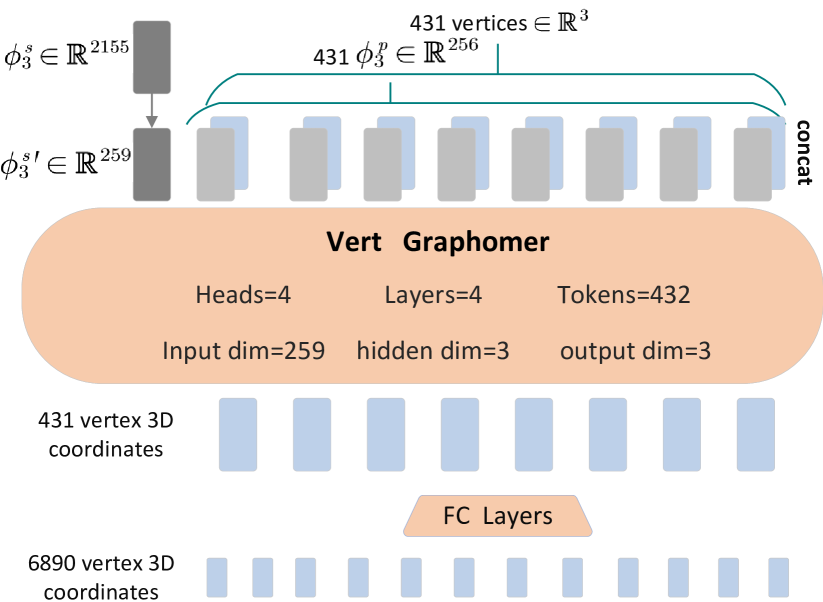
Figure 6: $\phi_{3}^{s}$ is first inputted into an FC layer to reduce its dimension to match the dimensions of other tokens. The 3D coordinates of the vertices are concatenated with their corresponding point-wise feature, forming a vertex query.

The parameter regressors consist of several FC layers and iteratively produce the final result like

$$\varTheta_{i}=\varTheta_{i-1}+FC\left(\oplus\left(\phi_{i}^{s},\,\,glob\_info,\ \varTheta_{i-1}\right)\right)$$ (13)

Note $\varTheta_{0}$ is set as the mean $\overline{\varTheta}$ following [14]. As for the final regressor, we have two versions in total. The first version still involves the parameter regressor. The second version utilizes a vertex regressor to obtain a finer human body mesh. After obtaining a coarse human mesh using the first two regressors, we introduce a model-free vertex regressor based on the transformer. As depicted in Fig. 6, this regressor takes spatial features $\phi_{3}^{s}$ and point-wise features $\phi_{3}^{p}$ as input. It’s important to note that no ”$fc$” exists in this case, indicating that these features do not undergo channel reduction. To reduce network complexity and adapt to the SMPL model, instead of directly recovering the 6890 vertices defined by SMPL, we recover 431 sparse vertices and gradually restore them to 6890 vertices using two linear layers.

8.3 Summary

We experiment with different backbones and downsampling points to validate our method and explore the optimal model structure. As a result, there are corresponding variations in the sizes of input images and features. We summarize these variations and create Tab 5 to provide an overview of these changes. The training process is conducted with a batch size of 128 and a fixed learning rate of 0.00005 on three RTX 3090 GPUs until convergence, taking approximately one week. Following [52, 18], we apply standard data augmentation techniques such as rotation, flipping, scaling, translation, noise, and occlusion. As for hyperparameters, $\lambda_{1}=\lambda_{2}=\lambda_{3}=300$, $\lambda_{4}=\lambda_{5}=\lambda_{6}=15$, $\lambda_{7}=0.06$,$\lambda_{8}=60$, $\lambda_{9}=0.03$ and $\lambda_{10}=\lambda_{11}=\lambda_{12}=0.05$.

9 About Metrics

We evaluate the reconstruction accuracy using 3D mesh vertices and joints. Specifically, for AGORA, we employ four metrics: MPJPE, MVE, NMJE, and NMVE. MPJPE stands for Mean Per Joint Position Error, which measures the accuracy of joint positions. For AGORA, it calculates the error for the first 24 SMPL joints after aligning with the root joint. Following [52, 20], we utilize 17 joints for MPI-INF-3D, while the other datasets employ a consistent set of 14 keypoints. MVE, or Mean Vertex Error, measures the error of all SMPL mesh vertices after aligning the root vertices. For other datasets except AGORA, PVE (Per Vertex Error) is computed without alignment. These metrics help assessing the accuracy of the reconstructed human bodies. NMJE (Normalized Mean Joint Error) and NMVE (Normalized Mean Vertex Error) are obtained by normalizing MPJPE and MVE using the F1 score. They provide an overall evaluation of the method’s performance, particularly in handling challenging scenarios. For specific calculation methods, please refer to [35].

As for the metrics in world coordinate, we follow SPEC [19] using W-MPJPE, PA-MPJPE, and W-PVE. PA-MPJPE (Procrustes-aligned Mean Per Joint Position Error) exists as a metric that purely evaluates the accuracy of body reconstruction. It removes the effect of unknown camera rotation by Procrustes-aligned and has therefore been adopted by many previous works. The calculation of W-MPJPE and W-PVE is not changed. The only difference is that the labels used are adjusted to the ground truth in world coordinate. We, including SPEC, believe that these metrics are more representative of the model’s capabilities in real-world applications.

10 More Experimental Results

Model	w/ 3DPW	3DPW
		MPJPE$\downarrow$	PA-MPJPE$\downarrow$	PVE$\downarrow$
HMR [14]	No	130.0	76.7	-
GraphCMR [21]	No	-	70.2	-
SPIN [20]	No	96.9	59.2	116.4
SPEC [19]	Yes	96.4	52.7	-
I2L-MeshNet [33]	No	93.2	57.7	110.1
Graphomer [26]	Yes	74.7	45.6	87.7
FastMETRO [4]	Yes	73.5	44.6	84.1
PyMAF [52]	Yes	92.8	58.9	110.1
VIBE [17]	No	93.5	56.5	113.4
VIBE [17]	Yes	82.9	51.9	99.1
PARE [18]	No	84.1	49.3	99.4
PARE [18]	Yes	79.1	46.4	94.2
HybrIK [23]	No	80.0	48.8	94.5
HybrIK [23]	Yes	74.1	45.0	86.5
Ours∗	No	75.6	46.7	87.7
Ours†	No	85.4	54.6	96.0
Ours-P†	No	82.9	52.1	95.1
Ours∗	Yes	68.5	43.2	81.6
Ours†	Yes	64.6	40.5	75.7
Ours-P†	Yes	67.3	41.6	79.9

Table 6: Comparison with SOTA Methods on 3DPW [42]. The column ”w/ 3DPW” indicates whether the model has been trained using the 3DPW dataset.

Model	H36M		MPI-INF-3D
	MPJPE$\downarrow$	PA-MPJPE$\downarrow$	MPJPE$\downarrow$	PA-MPJPE$\downarrow$
HMR [14]	88.0	56.8	124.2	89.8
GraphCMR [21]	-	50.1	-	-
SPIN [20]	62.5	41.1	105.2	67.5
PyMAF [52]	57.7	40.5	-	-
FastMETRO [4]	53.9	37.3	-	-
HMMR [15]	-	56.9	-	-
VIBE [17]	78.0	53.3	96.6	64.6
MEVA [30]	76.0	53.2	96.4	65.4
HybrIK [23]	54.4	34.5	-	-
CLIFF [25]	47.1	32.7	-	-
MPS-Net [44]	69.4	47.4	96.7	62.8
Ours∗	52.7	34.0	88.3	62.0
Ours†	51.0	29.8	83.2	59.1
Ours-P†	45.5	30.2	83.3	59.8

Table 7: Comparison with SOTA Methods on controllable datasets including Human 3.6M [12] and MPI-INF-3D [31].

Traditional Benchmarks Following previous methods [52, 44], we conduct evaluation on 3DPW [42], H36M [12], and MPII-INF-3D [31]. Specifically, we evaluate the performance of models trained with and without the 3DPW train set on the 3DPW test set. As shown in Tab 6, we achieve remarkable improvements on this challenging in-the-wild dataset, surpassing previous works easily. Even compared to the SOTA method HybrIK [23], W-HMR still exhibits significant advancements. However, in Tab 7, W-HMR’s performance is relatively less impressive in the case of controllable datasets, although it remains competitive with these SOTA methods. Controllable datasets refer to datasets obtained under laboratory conditions, typically characterized by limited variations in actors and scenes, which are prone to overfitting. HuMMan is also an example of such a dataset. So, it becomes difficult for our advantages to be fully demonstrated.

Design Details	AGORA
	NMVE$\downarrow$	NMJE$\downarrow$	MVE$\downarrow$	MPJPE$\downarrow$
sparse vertices	88.5	94.0	76.1	80.8
markers	84.7	89.7	72.8	77.1
3D bbox info	82.3	88.5	74.9	80.5
5D glob info	80.7	87.7	73.4	79.8
vert graphomer(indirect)	83.0	90.2	76.4	83.0
vert graphomer(direct)	82.4	88.6	75.8	81.5
1 param + 2 vert	82.0	91.0	70.5	78.3
2 param + 1 vert	82.9	89.5	71.0	77.0

Table 8: Ablation experiments regarding the design details of modules. The first comparison involves vertex selection for downsampling. The second comparison examines the impact of different information inputs. The third comparison evaluates different designs of the vert graphomer. The fourth comparison evaluates different combinations of regressors. Within each comparison, all settings remain consistent except for the variations in module design.

Figure 7: Qualitative results on HuMMan [3]. ”Input” refers to input images of the model. ”Overlay” means we project the recovered mesh back onto the original images. ”Cam” and ”World” show the output in camera and world coordinates, respectively.

Design Details To find the optimal design for our model, we conduct further ablation experiments. Firstly, we test different downsampling methods. Evidently, using markers for downsampling leads to better learning of human body features. Here, ”markers” refer to mocap markers. The improved performance might be because mocap markers serve as a better proxy for inferring human body information [55]. However, since using mocap markers conflicts with the vertex regressor, we only employ markers in the pure parameter regression.

We also compare our 5D global information with the 3D bounding box information proposed by CLIFF [25]. It is clear that, apart from the relative position information provided by the bounding box, the original image size also contains essential information for our task.

Additionally, we design different vertex regressors. One approach involves adding the output values to the input vertex coordinates to obtain the final results (indirect), while the other directly outputs the 3D vertex coordinates (direct). Evaluation results demonstrate that the direct approach is more efficient and effective.

Lastly, we test various combinations of the hybrid regression module. Both approaches show advantages, but it is apparent that the combination of ”2 param$+$1 vert” has clear benefits regarding model size and inference efficiency. Therefore, we ultimately select this combination as our final regression module.

Qualitative Results More visualizations are generated to give a more comprehensive reference. Also, we welcome running our codes on your samples. Back to qualitative results, from Fig. 9, we can see that our model is able to recover the human body very well when facing various scenes with various characters in various poses. We purposely show the results from multiple angles and in world space. In the past, many methods can also make the reconstructed mesh match the original image perfectly. But the reconstructed body doesn’t look good if we change the visual angle. Moreover, if we put it in the world space, the pose would behave abnormally.

It may not be noticeable from Fig. 9 because they fit the weak-perspective camera model and the assumption of $R_{c}=I$. But from Fig. 7, the drawbacks of the traditional method are undeniable. The reconstructed human body is entirely lopsided in world coordinate. But with our OrientCorrect module, the pose can be corrected very well to achieve a reasonable pose recovery in world coordinate. This method has a wide range of applications, allowing the model to reconstruct a proper human body when facing in-the-wild images. Of course, W-HMR is still not a perfect model, and for this reason, we show the failure cases in Fig. 8. We can find that our model is still not able to achieve accurate reconstruction when facing extreme poses (yoga, parkour), which may be due to the lack of relevant training data or may be limited by the iterative method. Secondly, when the human limbs are close to the body, there is often through-molding, which requires an extra optimization-based method to improve it or a human model with a higher degree of freedom. These will be one of the directions worth researching in the future.

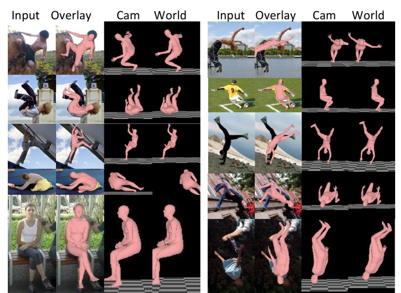
Figure 8: Failure cases on unusual samples. Although our model performs well in most cases, W-HMR still fails in some extreme situations. Such as, the human makes difficult poses, the body parts are hard to distinguish from the background, and the cross of limbs leads to mesh penetration.

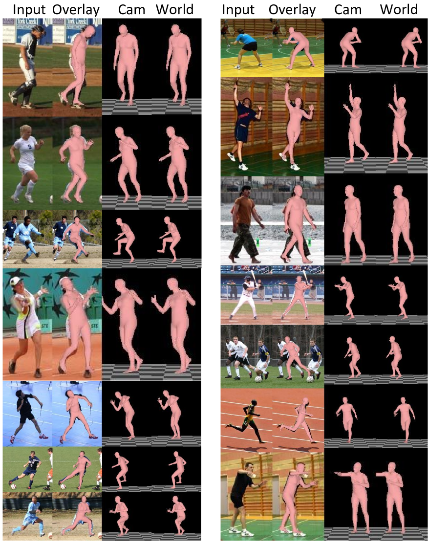
Figure 9: Qualitative results in camera and world coordinates. W-HMR shows excellent reconstruction accuracy and robustness. It is able to reconstruct various human bodies well in different scenes. Not only does the reconstructed mesh align well with the original image, but even when switching the angle of view, the reconstructed human body can still be seen to fit the target human.

References

- [1] Mykhaylo Andriluka, Leonid Pishchulin, Peter Gehler, and Bernt Schiele. 2d human pose estimation: New benchmark and state of the art analysis. In Proceedings of the IEEE Conference on computer Vision and Pattern Recognition, pages 3686–3693, 2014.
- [2] Dragomir Anguelov, Praveen Srinivasan, Daphne Koller, Sebastian Thrun, Jim Rodgers, and James Davis. Scape: shape completion and animation of people. In ACM SIGGRAPH 2005 Papers, pages 408–416. 2005.
- [3] Zhongang Cai, Daxuan Ren, Ailing Zeng, Zhengyu Lin, Tao Yu, Wenjia Wang, Xiangyu Fan, Yang Gao, Yifan Yu, Liang Pan, Fangzhou Hong, Mingyuan Zhang, Chen Change Loy, Lei Yang, and Ziwei Liu. HuMMan: Multi-modal 4d human dataset for versatile sensing and modeling. In 17th European Conference on Computer Vision, Tel Aviv, Israel, October 23–27, 2022, Proceedings, Part VII, pages 557–577. Springer, 2022.
- [4] Junhyeong Cho, Kim Youwang, and Tae-Hyun Oh. Cross-attention of disentangled modalities for 3d human mesh recovery with transformers. In European Conference on Computer Vision, pages 342–359. Springer, 2022.
- [5] Hongsuk Choi, Gyeongsik Moon, and Kyoung Mu Lee. Pose2mesh: Graph convolutional network for 3d human pose and mesh recovery from a 2d human pose. In Computer Vision–ECCV 2020: 16th European Conference, Glasgow, UK, August 23–28, 2020, Proceedings, Part VII 16, pages 769–787. Springer, 2020.
- [6] Alexey Dosovitskiy, Lucas Beyer, Alexander Kolesnikov, Dirk Weissenborn, Xiaohua Zhai, Thomas Unterthiner, Mostafa Dehghani, Matthias Minderer, Georg Heigold, Sylvain Gelly, et al. An image is worth 16x16 words: Transformers for image recognition at scale. arXiv preprint arXiv:2010.11929, 2020.
- [7] Qi Fang, Kang Chen, Yinghui Fan, Qing Shuai, Jiefeng Li, and Weidong Zhang. Learning analytical posterior probability for human mesh recovery. In Proceedings of the IEEE/CVF Conference on Computer Vision and Pattern Recognition, pages 8781–8791, 2023.
- [8] Shubham Goel, Georgios Pavlakos, Jathushan Rajasegaran, Angjoo Kanazawa, and Jitendra Malik. Humans in 4d: Reconstructing and tracking humans with transformers. arXiv preprint arXiv:2305.20091, 2023.
- [9] Chunhui Gu, Chen Sun, David A Ross, Carl Vondrick, Caroline Pantofaru, Yeqing Li, Sudheendra Vijayanarasimhan, George Toderici, Susanna Ricco, Rahul Sukthankar, et al. Ava: A video dataset of spatio-temporally localized atomic visual actions. In Proceedings of the IEEE conference on computer vision and pattern recognition, pages 6047–6056, 2018.
- [10] Rıza Alp Güler, Natalia Neverova, and Iasonas Kokkinos. Densepose: Dense human pose estimation in the wild. In Proceedings of the IEEE conference on computer vision and pattern recognition, pages 7297–7306, 2018.
- [11] Kaiming He, Xiangyu Zhang, Shaoqing Ren, and Jian Sun. Deep residual learning for image recognition. In Proceedings of the IEEE conference on computer vision and pattern recognition, pages 770–778, 2016.
- [12] Catalin Ionescu, Dragos Papava, Vlad Olaru, and Cristian Sminchisescu. Human3. 6m: Large scale datasets and predictive methods for 3d human sensing in natural environments. IEEE transactions on pattern analysis and machine intelligence, 36(7):1325–1339, 2013.
- [13] Hanbyul Joo, Natalia Neverova, and Andrea Vedaldi. Exemplar fine-tuning for 3d human model fitting towards in-the-wild 3d human pose estimation. In 2021 International Conference on 3D Vision (3DV), pages 42–52. IEEE, 2021.
- [14] Angjoo Kanazawa, Michael J Black, David W Jacobs, and Jitendra Malik. End-to-end recovery of human shape and pose. In Proceedings of the IEEE conference on computer vision and pattern recognition, pages 7122–7131, 2018.
- [15] Angjoo Kanazawa, Jason Y Zhang, Panna Felsen, and Jitendra Malik. Learning 3d human dynamics from video. In Proceedings of the IEEE/CVF conference on computer vision and pattern recognition, pages 5614–5623, 2019.
- [16] Imry Kissos, Lior Fritz, Matan Goldman, Omer Meir, Eduard Oks, and Mark Kliger. Beyond weak perspective for monocular 3d human pose estimation. In Computer Vision–ECCV 2020 Workshops: Glasgow, UK, August 23–28, 2020, Proceedings, Part II 16, pages 541–554. Springer, 2020.
- [17] Muhammed Kocabas, Nikos Athanasiou, and Michael J Black. Vibe: Video inference for human body pose and shape estimation. In Proceedings of the IEEE/CVF conference on computer vision and pattern recognition, pages 5253–5263, 2020.
- [18] Muhammed Kocabas, Chun-Hao P Huang, Otmar Hilliges, and Michael J Black. Pare: Part attention regressor for 3d human body estimation. In Proceedings of the IEEE/CVF International Conference on Computer Vision, pages 11127–11137, 2021a.
- [19] Muhammed Kocabas, Chun-Hao P Huang, Joachim Tesch, Lea Müller, Otmar Hilliges, and Michael J Black. Spec: Seeing people in the wild with an estimated camera. In Proceedings of the IEEE/CVF International Conference on Computer Vision, pages 11035–11045, 2021b.
- [20] Nikos Kolotouros, Georgios Pavlakos, Michael J Black, and Kostas Daniilidis. Learning to reconstruct 3d human pose and shape via model-fitting in the loop. In Proceedings of the IEEE/CVF international conference on computer vision, pages 2252–2261, 2019a.
- [21] Nikos Kolotouros, Georgios Pavlakos, and Kostas Daniilidis. Convolutional mesh regression for single-image human shape reconstruction. In Proceedings of the IEEE/CVF Conference on Computer Vision and Pattern Recognition, pages 4501–4510, 2019b.
- [22] Nikos Kolotouros, Georgios Pavlakos, Dinesh Jayaraman, and Kostas Daniilidis. Probabilistic modeling for human mesh recovery. In Proceedings of the IEEE/CVF international conference on computer vision, pages 11605–11614, 2021.
- [23] Jiefeng Li, Chao Xu, Zhicun Chen, Siyuan Bian, Lixin Yang, and Cewu Lu. Hybrik: A hybrid analytical-neural inverse kinematics solution for 3d human pose and shape estimation. In Proceedings of the IEEE/CVF conference on computer vision and pattern recognition, pages 3383–3393, 2021.
- [24] Yanghao Li, Hanzi Mao, Ross Girshick, and Kaiming He. Exploring plain vision transformer backbones for object detection. In European Conference on Computer Vision, pages 280–296. Springer, 2022a.
- [25] Zhihao Li, Jianzhuang Liu, Zhensong Zhang, Songcen Xu, and Youliang Yan. Cliff: Carrying location information in full frames into human pose and shape estimation. In European Conference on Computer Vision, pages 590–606. Springer, 2022b.
- [26] Kevin Lin, Lijuan Wang, and Zicheng Liu. Mesh graphormer. In Proceedings of the IEEE/CVF International Conference on Computer Vision, pages 12939–12948, 2021a.
- [27] Kevin Lin, Lijuan Wang, and Zicheng Liu. End-to-end human pose and mesh reconstruction with transformers. In Proceedings of the IEEE/CVF conference on computer vision and pattern recognition, pages 1954–1963, 2021b.
- [28] Tsung-Yi Lin, Michael Maire, Serge Belongie, James Hays, Pietro Perona, Deva Ramanan, Piotr Dollár, and C Lawrence Zitnick. Microsoft coco: Common objects in context. In Computer Vision–ECCV 2014: 13th European Conference, Zurich, Switzerland, September 6-12, 2014, Proceedings, Part V 13, pages 740–755. Springer, 2014.
- [29] Matthew Loper, Naureen Mahmood, Javier Romero, Gerard Pons-Moll, and Michael J Black. Smpl: A skinned multi-person linear model. ACM transactions on graphics (TOG), 34(6):1–16, 2015.
- [30] Zhengyi Luo, S Alireza Golestaneh, and Kris M Kitani. 3d human motion estimation via motion compression and refinement. In Proceedings of the Asian Conference on Computer Vision, 2020.
- [31] Dushyant Mehta, Helge Rhodin, Dan Casas, Pascal Fua, Oleksandr Sotnychenko, Weipeng Xu, and Christian Theobalt. Monocular 3d human pose estimation in the wild using improved cnn supervision. In 2017 international conference on 3D vision (3DV), pages 506–516. IEEE, 2017a.
- [32] Dushyant Mehta, Srinath Sridhar, Oleksandr Sotnychenko, Helge Rhodin, Mohammad Shafiei, Hans-Peter Seidel, Weipeng Xu, Dan Casas, and Christian Theobalt. Vnect: Real-time 3d human pose estimation with a single rgb camera. Acm transactions on graphics (tog), 36(4):1–14, 2017b.
- [33] Gyeongsik Moon and Kyoung Mu Lee. I2l-meshnet: Image-to-lixel prediction network for accurate 3d human pose and mesh estimation from a single rgb image. In Computer Vision–ECCV 2020: 16th European Conference, Glasgow, UK, August 23–28, 2020, Proceedings, Part VII 16, pages 752–768. Springer, 2020.
- [34] Gyeongsik Moon, Hongsuk Choi, and Kyoung Mu Lee. Accurate 3d hand pose estimation for whole-body 3d human mesh estimation. In Proceedings of the IEEE/CVF Conference on Computer Vision and Pattern Recognition, pages 2308–2317, 2022.
- [35] Priyanka Patel, Chun-Hao P. Huang, Joachim Tesch, David T. Hoffmann, Shashank Tripathi, and Michael J. Black. AGORA: Avatars in geography optimized for regression analysis. In Proceedings IEEE/CVF Conf. on Computer Vision and Pattern Recognition (CVPR), 2021.
- [36] Georgios Pavlakos, Vasileios Choutas, Nima Ghorbani, Timo Bolkart, Ahmed AA Osman, Dimitrios Tzionas, and Michael J Black. Expressive body capture: 3d hands, face, and body from a single image. In Proceedings of the IEEE/CVF conference on computer vision and pattern recognition, pages 10975–10985, 2019.
- [37] Gerard Pons-Moll, Javier Romero, Naureen Mahmood, and Michael J Black. Dyna: A model of dynamic human shape in motion. ACM Transactions on Graphics (TOG), 34(4):1–14, 2015.
- [38] Chris Rockwell and David F Fouhey. Full-body awareness from partial observations. In Computer Vision–ECCV 2020: 16th European Conference, Glasgow, UK, August 23–28, 2020, Proceedings, Part XVII 16, pages 522–539. Springer, 2020.
- [39] Karthik Shetty, Annette Birkhold, Srikrishna Jaganathan, Norbert Strobel, Markus Kowarschik, Andreas Maier, and Bernhard Egger. Pliks: A pseudo-linear inverse kinematic solver for 3d human body estimation. In Proceedings of the IEEE/CVF Conference on Computer Vision and Pattern Recognition, pages 574–584, 2023.
- [40] Yating Tian, Hongwen Zhang, Yebin Liu, and Limin Wang. Recovering 3d human mesh from monocular images: A survey. arXiv preprint arXiv:2203.01923, 2022.
- [41] Gul Varol, Duygu Ceylan, Bryan Russell, Jimei Yang, Ersin Yumer, Ivan Laptev, and Cordelia Schmid. Bodynet: Volumetric inference of 3d human body shapes. In Proceedings of the European conference on computer vision (ECCV), pages 20–36, 2018.
- [42] Timo Von Marcard, Roberto Henschel, Michael J Black, Bodo Rosenhahn, and Gerard Pons-Moll. Recovering accurate 3d human pose in the wild using imus and a moving camera. In Proceedings of the European Conference on Computer Vision (ECCV), pages 601–617, 2018.
- [43] Wenjia Wang, Yongtao Ge, Haiyi Mei, Zhongang Cai, Qingping Sun, Yanjun Wang, Chunhua Shen, Lei Yang, and Taku Komura. Zolly: Zoom focal length correctly for perspective-distorted human mesh reconstruction. arXiv preprint arXiv:2303.13796, 2023.
- [44] Wen-Li Wei, Jen-Chun Lin, Tyng-Luh Liu, and Hong-Yuan Mark Liao. Capturing humans in motion: Temporal-attentive 3d human pose and shape estimation from monocular video. In Proceedings of the IEEE/CVF Conference on Computer Vision and Pattern Recognition, pages 13211–13220, 2022.
- [45] Jiahong Wu, He Zheng, Bo Zhao, Yixin Li, Baoming Yan, Rui Liang, Wenjia Wang, Shipei Zhou, Guosen Lin, Yanwei Fu, et al. Large-scale datasets for going deeper in image understanding. In 2019 IEEE International Conference on Multimedia and Expo (ICME), pages 1480–1485. IEEE, 2019.
- [46] Hongyi Xu, Eduard Gabriel Bazavan, Andrei Zanfir, William T Freeman, Rahul Sukthankar, and Cristian Sminchisescu. Ghum & ghuml: Generative 3d human shape and articulated pose models. In Proceedings of the IEEE/CVF Conference on Computer Vision and Pattern Recognition, pages 6184–6193, 2020.
- [47] Yufei Xu, Jing Zhang, Qiming Zhang, and Dacheng Tao. Vitpose: Simple vision transformer baselines for human pose estimation. Advances in Neural Information Processing Systems, 35:38571–38584, 2022a.
- [48] Yufei Xu, Jing Zhang, Qiming Zhang, and Dacheng Tao. Vitpose+: Vision transformer foundation model for generic body pose estimation. arXiv preprint arXiv:2212.04246, 2022b.
- [49] Andrei Zanfir, Eduard Gabriel Bazavan, Mihai Zanfir, William T Freeman, Rahul Sukthankar, and Cristian Sminchisescu. Neural descent for visual 3d human pose and shape. In Proceedings of the IEEE/CVF Conference on Computer Vision and Pattern Recognition, pages 14484–14493, 2021a.
- [50] Mihai Zanfir, Andrei Zanfir, Eduard Gabriel Bazavan, William T Freeman, Rahul Sukthankar, and Cristian Sminchisescu. Thundr: Transformer-based 3d human reconstruction with markers. In Proceedings of the IEEE/CVF International Conference on Computer Vision, pages 12971–12980, 2021b.
- [51] Hongwen Zhang, Jie Cao, Guo Lu, Wanli Ouyang, and Zhenan Sun. Learning 3d human shape and pose from dense body parts. IEEE Transactions on Pattern Analysis and Machine Intelligence, 2020a.
- [52] Hongwen Zhang, Yating Tian, Xinchi Zhou, Wanli Ouyang, Yebin Liu, Limin Wang, and Zhenan Sun. Pymaf: 3d human pose and shape regression with pyramidal mesh alignment feedback loop. In Proceedings of the IEEE/CVF International Conference on Computer Vision, pages 11446–11456, 2021a.
- [53] Hongwen Zhang, Yating Tian, Yuxiang Zhang, Mengcheng Li, Liang An, Zhenan Sun, and Yebin Liu. Pymaf-x: Towards well-aligned full-body model regression from monocular images. IEEE Transactions on Pattern Analysis and Machine Intelligence, 2023.
- [54] Tianshu Zhang, Buzhen Huang, and Yangang Wang. Object-occluded human shape and pose estimation from a single color image. In Proceedings of the IEEE/CVF conference on computer vision and pattern recognition, pages 7376–7385, 2020b.
- [55] Yan Zhang, Michael J Black, and Siyu Tang. We are more than our joints: Predicting how 3d bodies move. In Proceedings of the IEEE/CVF Conference on Computer Vision and Pattern Recognition, pages 3372–3382, 2021b.
- [56] Zerong Zheng, Tao Yu, Yixuan Wei, Qionghai Dai, and Yebin Liu. Deephuman: 3d human reconstruction from a single image. In Proceedings of the IEEE/CVF International Conference on Computer Vision, pages 7739–7749, 2019.
- [57] Silvia Zuffi and Michael J Black. The stitched puppet: A graphical model of 3d human shape and pose. In Proceedings of the IEEE Conference on Computer Vision and Pattern Recognition, pages 3537–3546, 2015.