1

A Categorical Framework for Quantifying
Emergent Effects in Network Topology

Johnny Jingze Li^1,2, Sebastian Prado Guerra^1,2,3, Kalyan Basu⁴, Gabriel A. Silva^1,3,5
1Center for Engineered Natural Intelligence, University of California San Diego, La Jolla, CA, United States
²Department of Mathematics, University of California San Diego, La Jolla, CA, United States
³Department of Bioengineering, University of California San Diego, La Jolla, CA, United States
⁴Microsoft, Technology & Research, Redmond, WA, USA
⁵Department of Neurosciences, University of California San Diego, La Jolla, CA, United States

Keywords: emergence, homological algebra, derived functor, cohomology, quiver representation, random Boolean network

Emergent effect is crucial to the understanding of the properties of complex systems that do not appear in their basic units, but there has been a lack of theories to measure and understand its mechanisms. In this paper, we established a framework based on homological algebra that encodes emergence as the mathematical structure of cohomologies and then applied it to network models to develop a computational measure of emergence. This framework ties the emergence of a system to its network topology and local structures, paving the way to predict and understand the cause of emergent effects. We show in our numerical experiment that our measure of emergence correlates with the existing information-theoretic measure of emergence.

1 Introduction

Emergent effects of complex systems are, broadly speaking, phenomena present in the system that are not shared by and cannot be explained by an understanding or considerations of the system’s constituent components in isolation. This is often expressed as ’the whole is more than the sum of its parts’. The concept of emergence in complex systems has been a topic of extensive study and is of importance across most of the natural and physical sciences, and increasingly in engineering (Anderson, 1972; Kalantari et al., 2020; Post & Weiss, 1997; O’Connor, 2020; Forrest, 1990).

While there is no universally accepted technical definition of emergence, there are a number of intuitive ideas and concepts that capture its essence and find commonality across disciplines. Probably the most important is the notion that novel properties, patterns, or behaviors that are not explicitly or predictably present in the constituent parts that make up a system, or in the interactions between the parts. This phenomenon captures the idea that emergent properties are not reducible to or explainable solely by the properties of individual components, but rather, arise from the interactions and organization of those components within the system in highly non-obvious ways. It also emphasizes the non-linearity and unpredictability associated with emergence.

Surprisingly, with the recent performance of large language models, emergence is also becoming an important topic in machine learning and artificial intelligence. Researchers have observed a surge in performance when the scale of these models reached a certain threshold that could not be predicted by extrapolation (see, e.g., Wei et al., 2022; Teehan et al., 2022). This new work is opening up novel and exciting research avenues to explore, and hopefully eventually explain, the unreasonable effectiveness of massive deep learning architectures.

Still, a clear limitation of current work on emergence across essentially all fields and applications is that they remain at a phenomenological level, for example, the shift of system behavior with an increasing number of computational units. The kind of measures derived from observation of such macroscopic effects do not result in mechanistic insights into why such emergence occurs, or how to anticipate and predict it. To address this, we need new measures that can describe and predict emergence on a more fundamental level capable of incorporating structural information and interactions between components (see, e.g., Barabasi & Oltvai, 2004). Grounded in a mechanistic understanding of emergence with measures that capture causal relationships, new theoretical models and numerical simulations might be able to explain how system structure changes when emergent effects occur. Eventually, this might support the intentional engineering of emergent effects.

There have been a number of attempts at establishing frameworks that describe and measure emergence (e.g. Crutchfield, 1994; Bar-Yam, 2004; Gadioli La Guardia & Jeferson Miranda, 2018; Gershenson & Fernández, 2012; Correa, 2020; Green, 2023; Mediano et al., 2022). Some approaches are based on information-theoretic notions, but in most cases the structure and interactions between participating components are not explicitly included in the computation of emergence, thus falling short of providing mechanistic insights. The challenge is in connecting the level of observations where researchers study complexity of structures, patterns or dynamics with the more fundamental level of interacting components which give rise to emergent effects, and how to represent interactions in a way that is effective and easy to compute. As such, a universal and computable measure of emergence applicable to real-world systems still does not exist.

Notably, in Adam (2017), these shortcomings are partially addressed by studying the functor that connects two levels and proving that the approach to quantify emergence as the non-commutativity of algebraic operations is equivalent to a ”loss of exactness” which we progressively describe in our paper — in the sense that the interactions between components are represented through the morphisms and colimits of a category. We show that observing the algebraic properties of the derived functor on that category is sufficient to capture and describe emergence. This new perspective thus supports more effective ways of quantifying emergence in a practical setting.

Our work in this paper builds on the work by Adam (2017). Specifically, we establish a framework for studying and evaluating emergence — which we refer to as generativity to be more precise — that incorporates both an abstract mathematical framework and a practical computational metric capable of being applied to real-world systems such as networks. For example, we will show that our framework can potentially be used to study the emergent properties of massive deep-learning architectures. Essentially, a system’s ability to sustain emergent effects is represented as the mathematical structure of derived functor and cohomologies which are computable. Algebraic tools can then be applied to further investigate emergent effects. Compared with numerical metrics that evaluate emergence, our framework is richer in information, as the algebraic structure encodes more structural information about the system, for example, the contribution of each component to emergence as the global property of the system, thus supports an increased understanding of the mechanistic details resulting in emergent phenomena. We then compare this framework with existing information-theoretic measure of emergence through numerical experiment on networks of different connectivities and show a correlation that supports the ability of our theory to capture emergence generally.

The following sections are organized as follows: In Section 2 we define and illustrate emergent effects through an example, in Section 3, we present the framework for emergence as loss of exactness, adapted from Adam (2017). In Section 4 and 5, this framework is realized as the mapping between networks, or more generally, quiver representations and then we compute the mathematical structure which encodes emergence. In Section 6 we establish the numerical measure of emergence and then discuss the numerical result showing a correlation with existing measures of emergence.

2 A Descriptive Framework for Emergent Effects

Two key conceptual components are necessary to qualitatively describe emergent effects within the framework proposed by Adam (see Adam, 2017). The first is a notion of interaction or interconnection between the components of a system. For example, a thermodynamics system consisting of particles exhibits interesting properties because of the interactions between particles. The second is the notion of interactional effects, which equips each system with an observable. For example, we perceive and can feel hot or cold, and can measure temperature, due to the interactions between particles, but not from the observation or description of any number of individual particles. These kinds of interactional effects are almost always associated with partial observations, or a simplification and integration of lower — more foundational or granular —levels or scales in the system that result in a ’loss of information’ or inability to properly observe the effects of those interactions at a higher level.

With these two ingredients, we can define emergence as a partial observation of interacting and interconnected components within a system that cannot be explained by known interactions that produce or result in partial observations of the components. This notion agrees with the intuative understanding of emergence that some properties of the interconnected components cannot be decomposed or reduced to combinations of known properties of the constituent components, i.e. that the whole is more than the sum of its parts. This notion of emergence is the foundation on which our work in this paper, building on the framework first proposed in Adam (2017), develops a mathematical definition and computational measure of emergence.

To formalize these ideas, we begin by representing the interactions between components as an operation $\vee$, where $s_{1}\vee s_{2}$ represents a new interconnected system of subsystems $s_{1}$ and $s_{2}$. Interactional effects are described by the mapping $\Phi$ between a system and its partial observation from a higher level. Mathematically then,

Definition 2.1.

Emergence occurs in a system when the following inequality is satisfied:

$$\Phi(s_{1}\vee s_{2})\neq\Phi(s_{1})\vee\Phi(s_{2}),$$ (1)

for some constituent subsystems $s_{1}$ and $s_{2}$.

The reader should note that while similar qualitative notions of emergence have been used in other work (Bar-Yam, 2004; Gadioli La Guardia & Jeferson Miranda, 2018; Green, 2023; Mediano et al., 2022), their use of these concepts to describe a formal notion of emergence falls short. As far as we are aware, no prior attempts have resulted in a quantity based on definition 2.1 that directly produces a measure of emergence. Adam (2017) attempted to address this issue, and we will discuss it in the next section by proposing emergence as ”the loss of exactness”, a term from homological algebra.

Note that the definition given above is also related to the notion of emergence as defined in engineering, for example, Wei et al. (2022), as the new properties/ abilities of the system when the size of the model increases. If we consider $s_{1}$ and $s_{2}$ as two smaller models, $s_{1}\vee s_{2}$ as combining two smaller models into a larger model by, for example, techniques in ensemble learning, (see, e.g., Mohammed & Kora, 2023), and $\Phi$ as the mapping that reflects the properties/ abilities of the model, then $\Phi(s_{1}\vee s_{2})$ is the properties/ abilities of the combined model and $\Phi(s_{1})\vee\Phi(s_{2})$ can be interpreted as a summation of the properties/ abilities of each small model. Then the difference between $\Phi(s_{1}\vee s_{2})$ and $\Phi(s_{1})\vee\Phi(s_{2})$ can reflect the emergent properties/ abilities that result in the nonlinear increase of performance, related to the performance in Wei et al. (2022).

In the rest of this section we give an example that illustrates the notion of emergence as in definition 2.1. This example is inspired by a pseudo-type learning process in which the learner is able to extract only partial information from the input data, represented here as a temporally associated network of sequentially presented images.

We start by defining each system as a time lapse sequence of images (although they could be any other data units) $\{\Lambda_{i}\}_{i\in\mathbb{Z}}$ endowed with similarity values between any two images whenever the first image precedes the second image. In other words, we will have a similarity value $\omega_{i,j}$ between the images $\Lambda_{i}$ and $\Lambda_{j}$ if, and only if, $i<j$ in $\mathbb{Z}$.

Figure 1: Each system is a network structure

When two systems $s,s^{\prime}$ share some common parts, the interaction $\vee$ is defined as gluing the two sequences and the establishment of interconnecting dashed arrows (in blue):

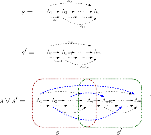
Figure 2: The interaction of two systems as glueing the two network structures together and establishing the interconnecting arrows.

In Figure 2, system $s$ and $s^{\prime}$ has a common element $\Lambda_{n}$ and the interconnected system of $s$ and $s^{\prime}$ is defined as the structure $s\vee s^{\prime}$, where we glued $s$ and $s$ together, and then adding the arrows from elements in $s$ to elements in $s^{\prime}$, thus making $s\vee s^{\prime}$ a new system.

When doing partial observation of a network structure, it is likely that some edges, in some contexts especially long-range edges are not captured. So as an option we can construct $\Phi$ such that the edges longer than $\delta$ is being neglected:

$$\Phi_{\delta}(\omega_{ij})=\left\{\begin{array}[]{rcl}\omega_{ij}&\mbox{when}&|i-j|\leq\delta\\ \\ 0&\mbox{when}&|i-j|>\delta\end{array}\right.$$ (5)

here $\delta$ acts like the attention span of an information processing system beyond which the connections are no longer able to be captured. As an example, $\Phi_{2}$ will neglect all the edges of length greater than $2$, thus  

Figure 3: An example of $\Phi(s)$ as partial observation to system $s$.

Now, whether there is emergent effect or not depend on the interaction $\vee^{\prime}$ between two partial observations $\Phi(s)\vee^{\prime}\Phi(s^{\prime})$. When $\vee^{\prime}$ is the same as $\vee$, the interaction rule between two systems as defined in Figure 2, we can see that there is indeed emergent effect, because $\Phi(s)\vee^{\prime}\Phi(s^{\prime})$ will still recover the long-range edges between elements in $\Phi(s)$ and $\Phi(s^{\prime})$ which are not presented in $\Phi(s\vee s^{\prime})$ because the truncation effect of $\Phi$, illustrated in Figure 4.

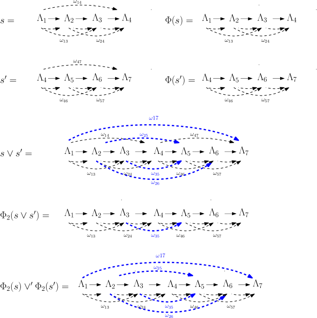
Figure 4: An example of emergent effect showing $\Phi(s\vee s^{\prime})\neq\Phi(s)\vee^{\prime}\Phi(s^{\prime})$

This produces a family of functors $\Phi_{\delta}$ satisfying $\Phi_{\delta}(s)\vee^{\prime}\Phi_{\delta}(s^{\prime})\neq\Phi_{\delta}(s\vee s^{\prime})$. Intuitively, under this choice of interaction of observations $\vee^{\prime}$, the smaller the attention span $\delta$ is, the more different $\Phi_{\delta}(s\vee s^{\prime})$ will be from $\Phi_{\delta}(s)\vee\Phi_{\delta}(s^{\prime})$, with more dashed arrows truncated. Note that there are other choices of $\vee^{\prime}$, for example, when $\Phi(s)$ interacts with $\Phi(s^{\prime})$, not necessarily all edges between $\Phi(s)$ and $\Phi(s^{\prime})$ can be recovered. In this case, there could be no emergent effect, for example, when no edges longer than $\delta$ can be recovered, then $\Phi(s)\vee^{\prime}\Phi(s^{\prime})=\Phi(s\vee s^{\prime})$.

This example provides a high-level illustration of emergent effects according to our definition in definition 2.1. The partial observation $\Phi$ that leads to interactional effects is defined by ”forgetting edges” which induces the concept of an attention span. In this example, the emergent effect is related to the length of the attention span. The shorter the attention span, the more $\Phi(s\vee s^{\prime})$ will differ from $\Phi(s)\vee\Phi(s^{\prime})$. In the following sections of this paper, we will build a framework based on category theory that gives a theoretical analysis of this observation.

Importantly, if this difference is viewed as a kind of information loss, this consideration agrees with certain information-theoretic results for networks. For example, Gershenson & Fernández (2012) has shown through simulations that networks with poor connectivity (shorter attention span) lead to greater information loss. In Section 5 and 6 we will demonstrate this in our theory and numerical experiments. But first, in the next section, we formulate this approach in a more tractable way in order to produce an effective computational measure.

3 Emergence as loss of exactness

In this section we reformulate the intuitive concepts of emergence introduced in the previous sections in a way that leads to an effective quantitative measure. We say that a system is emergent if there exist two components satisfying the condition that $\Phi(s_{1}\vee s_{2})\neq\Phi(s_{1})\vee\Phi(s_{2})$. However, as discussed in the introduction, on its own this definition of emergence is not sufficient to evaluate the amount of emergent effects that can present in a system. We need to approximate the difference when $\Phi(s_{1}\vee s_{2})$ and $\Phi(s_{1})\vee\Phi(s_{2})$ are representing two non-numerical structures, for example, networks. Also we hope to have a global measure of emergence of a system that takes into account all its subsequent components $s_{i}$. Importantly, Adam (2017) proved that emergence can be formulated as ”loss of exactness”, a notion in homological algebra. This perspective has a number of advantages for quantifying emergence, which we progressively discuss in detail in this section.

Adam (2017) adopted an algebraic approach to describe emergent effects through interactions among the components, formulated in the language of category theory. The use of category theory in other than pure math is gaining increasing traction and producing some interesting tools and insights (see, e.g., Rosen, 1958a, b; Bradley, 2018; Fong & Spivak, 2018; Northoff et al., 2019). In Adam (2017), the use of category theory is natural since the Abelian category is foundational to the tools and constructions of homological algebra.

A category is an algebraic structure consisting of objects and morphisms. We consider the collection of subsystems and their constituent components that give rise to emergent effects as the category System, where each object is a subsystem. The morphisms represent a relation between subsystems to be interpreted, for example, $f:V\rightarrow W$ can give a way to embed subsystem $V$ into $W$. When subsystems interact they form a new subsystem (we also call it interconnection). This new resultant subsystem is captured as the mathematical concept of colimit with respect to the interaction diagram, which is treated in detail in Fong & Spivak (2018). Colimit is an object in System, as defined below, that satisfies certain properties. In Section 4 we discuss the category of quiver representations as System and we will give the colimit and see how it can be regarded as interconnection among objects.

Definition 3.1.

A co-cone of a diagram $F:J\rightarrow C$ is an object $N$ in $C$ together with a family of morphisms

$$\phi_{X}:F(X)\rightarrow N$$ (6)

for every object $X$ of $J$, such that for every morphism $f:X\rightarrow Y$ in $J$, we have $\phi_{Y}\circ F(f)=\phi_{X}$.

Definition 3.2.

A colimit of a diagram $F:J\rightarrow C$ is a co-cone $(L,\phi_{X})$ such that for any other co-cone $(N,\psi)$ of $F$ there exists a unique morphism $u:L\rightarrow N$ such that $u\circ\phi_{X}=\psi_{X}$ for all $X$ in $J$.

There are several candidates of diagrams $F$ to model the interconnected system $s_{1}\vee s_{2}$ as the colimit of $F$. One option would be pushouts, namely when $J$ is of the form $\bullet\leftarrow\bullet\rightarrow\bullet$. The interaction of $s_{1}$ and $s_{2}$ can be regarded as the pushout diagram:

where $s_{0}$ can be interpreted as the part that $s_{1}$ and $s_{2}$ share in common after the interaction. In Adam (2017), the diagram $F$ is also called the interaction blueprint, and we have the following definition for interaction in the category theory context:

Definition 3.3.

(Definition 8.3.2 in Adam (2017)) The system resulting from the interaction along a diagram $F$ is the object $\varinjlim F$ of the colimit of the diagram $F$.

The partial observations of the system are represented by a functor $\Phi:\textbf{System}\rightarrow\textbf{Phenome}$, where Phenome is another category whose objects are the observations of objects in System. Now we can translate the definition 2.1 of emergence into the category theory setting:

Definition 3.4.

(Definition 8.3.5 in Adam (2017)) A functor $\Phi$ sustains emergence effects if and only if the map $\varinjlim\Phi F\rightarrow\Phi\varinjlim F$ is not an isomorphism for some diagram $F$.

In this way, we have redefined emergence as not preserving some colimit. In category theory terms, this is equivalent to saying that the functor $\Phi$ is not a co-contiuos functor. In the following we are going to show that the extent to which colimit is not preserved is reflected as the loss of exactness.

The framework we develop here is based on a special case of this general framework, specifically, we consider the case when both System and Phenome are Abelian categories, a category in which morphisms and objects can be added and in which kernels and cokernels exist and have desirable properties, for a detailed definition, see (Mac Lane, 2013). Basic examples include the category of Abelian groups, and the category of vector spaces over a field $k$. On Abelian categories, the constructions of homological algebra are available, including exact sequences, to which we can relate an interaction process.

In Freyd (1964) Proposition 2.5.3 the following result has been proven:

Proposition 3.5.

In an Abelian category, the square

is a pushout if and only if the sequence

is exact.

where exact is defined as

Definition 3.6.

A sequence is exact when it is exact at $A$ and $A^{\prime}$ and $A^{\prime\prime}$, which means ${\rm Im}a=\ker f$ and ${\rm Im}f=\ker g$ and ${\rm Im}g=\ker b$.

The notion of exactness is fundamental in homological algebra, and we can extend this to functors:

Definition 3.7.

A functor $\Phi$ is exact when it maps an exact sequence

(7)

to another exact sequence. In other words, the following sequence is exact:

(8)

Furthermore, $\Phi$ is left exact if

(9)

is exact, and $\Phi$ is right exact if

(10)

is exact.

In this context, Adam (2017) proved the following result:

Proposition 3.8.

(Proposition 8.4.3 in Adam (2017)) Assume the functor $\Phi$ between two Abelian categories is additive and left exact. Then $\Phi$ sustains emergent effects if and only if for some exact sequence $A\rightarrow A^{\prime}\rightarrow A^{\prime\prime}\rightarrow 0$, the sequence $\Phi(A)\rightarrow\Phi(A^{\prime})\rightarrow\Phi(A^{\prime\prime})\rightarrow 0$ is not exact at either $\Phi(A^{\prime})$ or $\Phi(A^{\prime\prime})$.

What this proposition achieves is encoding emergent effects as a loss of exactness when a sequence in System is mapped into Phenome. We can take advantage of this fact to develop a measure of emergence that is based on a loss of exactness as developed in homological algebra, which describes the mathematical mahinery to quantify loss of exactness Gelfand & Manin (2013).

Homological algebra is often regarded as a mathematical bridge between the worlds of topology and algebra. It is the study of homological functors and the intricate algebraic structures that they entail; its development was closely intertwined with the emergence of category theory. A central concept is that of specific sequences, referred to as chain complexes, that can be studied through both their homology and cohomology. Homological algebra is capable of extracting information contained in these complexes and presenting them in the form of homological invariants of rings, modules, topological spaces, and other ’tangible’ mathematical objects which have their own further structure, properties, and interpretations Cartan & Eilenberg (1999); Gelfand & Manin (2013).

Within this framework of homological algebra, a loss of exactness can be encoded in the derived functor introduced below. This approach evaluates emergence via the algebraic properties of the functor itself. Given a function (or more generally a functor) $\Phi$ on a set (category) of networks that represents the processing of information in a system, we can extract information from the ”derivative” of the function (derived functor), represented as $L^{1}\Phi$ or $R^{1}\Phi$ in the standard literature. Now we show they encode information related to emergence.

Let System and Phenome both be abelian categories and assume $\Phi$ is one-side exact. For example, in this section we assume $\Phi$ is left exact and not right exact, thus admitting non-trivial right derived functors $R^{n}\Phi$. Recall that given an object $A$ in System, if we pick an injective resolution, which is by definition an exact sequence:

(11)

then we recover a chain complex:

(12)

Then we define $R^{i}\Phi(A)$ to be the $i$th cohomology object of the complex (similarly, $L^{i}\Phi(A)$ is defined as the $i$th cohomology object of the complex recovered from the projective resolution). Standard textbooks in homological albgera, for example, Rotman & Rotman (2009) has shown that they are indeed functors, and under the assumption that $\Phi$ is left-exact, we have $R^{0}\Phi(A)=\Phi(A)$. In Section 5 we will give a concrete definition and example that finds $L^{1}\Phi(A)$ and $R^{1}\Phi(A)$. Now note that the chain complex (12) we recovered is not necessarily exact. To measure how much exactness is lost under this functor, we can take advantage of the following standard result in homological algebra (see, e.g. Gelfand & Manin, 2013), which gives us a long exact sequence

Proposition 3.9.

Given an exact sequence

(13)

in System, the following long exact sequence is exact:

(14)

This means, if $R^{1}\Phi(A)=0$, the sequence

(15)

is right exact, which means no emergence is sustained. Thus the first derived functor $R^{1}\Phi$ encodes the potential of a system to sustain emergent effects.

This observation provides the foundation for us to mathematically compute the emergence of systems of interest by connecting emergence with a derived functor. The emergence of a specific system $A$ will be determined by the image of this system under the derived functor, represented as $R^{1}\Phi(A)$. Note that this gives us a global representation of emergence, not specific to the choice of interacting parts $s_{1},s_{2}$ in definition 2.1.

In this section we assumed $\Phi$ to be left exact, and thus the first right derived functor $R^{1}\Phi$ encodes the emergence. In the case when $\Phi$ is right exact, it will admit left derived functors $L^{n}\Phi$ and now $L^{1}\Phi$ encodes the emergence. We will discuss in detail in Section 5, where we compute $L^{1}\Phi$ and $R^{1}\Phi$ explicitly.

We need to introduce a particlar constraint to this framework before we can use it to study the emergence of any specific system. In the analysis above, we necessarily assumed that the System category is an Abelian category, or is lifted to an Abelian category, because these types of categories have properties that support the formation of exact sequences. From a practical perspective in order to implement this constraint, in the next two sections we consider the more general category System introduced in Section 2 to be the category of quiver representations. It can be used to model network structures. It is an Abelian category and its homological algebra has been developed (e.g. Derksen & Weyman, 2017).

4 Quiver representations

In this section, we introduce quiver representation as an effective way to represent network systems and a bridge that connects the abstract homologcial algebra framework in the previous section with applicable measure of emergence. As a pre-step to compute $L^{1}\Phi(A)$ or $R^{1}\Phi(A)$ which encodes the emergence of a system $A$, we realize the category System as the category of quiver representations $\textbf{Rep}(Q)$, where each object in System is a quiver representation of a quiver $Q$. A quiver representation is the mathematical structure obtained by considering network nodes as vector spaces and edges as linear maps. Related work by other authors have explored the connection between quiver representations, neural networks, and data representations (see, e.g., Armenta & Jodoin, 2021; Parada-Mayorga et al., 2020; Ganev & Walters, 2022).

Quiver representation has the following advantages: first, the category of quiver representations $\textbf{Rep}(Q)$ is itself an Abelian category, the kind of category on which we can carry out homological algebra constructions. Second, plenty of mathematical theories on quiver representations and quiver varieties (see, e.g., Kirillov Jr, 2016; Jeffreys & Lau, 2022) have been developed that can potentially be applied to the formulation of neural networks. Third, the representation of nodes and edges can potentially be used to model information flow on the network and encode the biophysics that govern those networks.

Formally, a quiver is a directed graph where multiple edges and loops are allowed, defined as follows:

Definition 4.1.

A quiver $Q$ is a quadruple $Q=(Q_{0},Q_{1},h,t)$ where $Q_{0}$ is a finite set of vertices, $Q_{1}$ is a finite set of arrows, and $h$ and $t$ are functions $Q_{1}\rightarrow Q_{0}$. For an arrow $a\in Q_{1}$, $h(a)$ and $t(a)$ are called the head and tail of $a$.

Definition 4.2.

We get a representation $V$ of $Q=(Q_{0},Q_{1},h,t)$ if we attach to every vertex $x\in Q_{0}$ a finite dimentional $\mathbb{C}$-vector space $V(x)$ and to every arrow $a\in Q_{1}$ a $\mathbb{C}$-linear map $V(a):V(ta)\rightarrow V(ha)$.

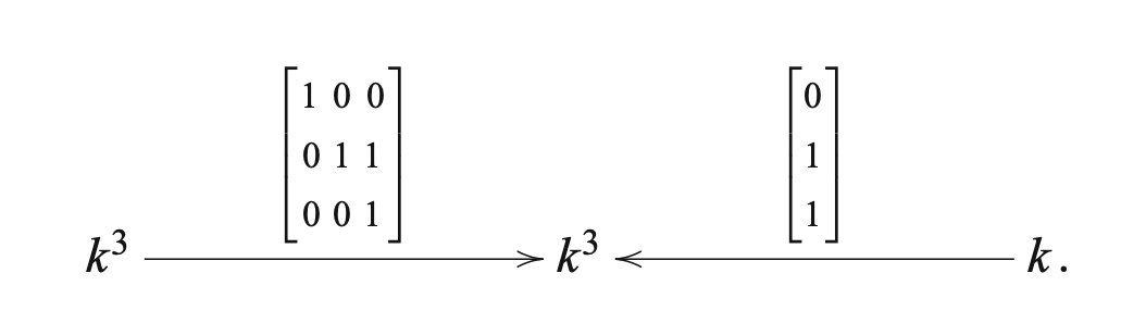
Figure 5: A simple example of representation of quiver $\bullet\rightarrow\bullet\leftarrow\bullet$ over a field $k$. Adapted from Schiffler, (2014)

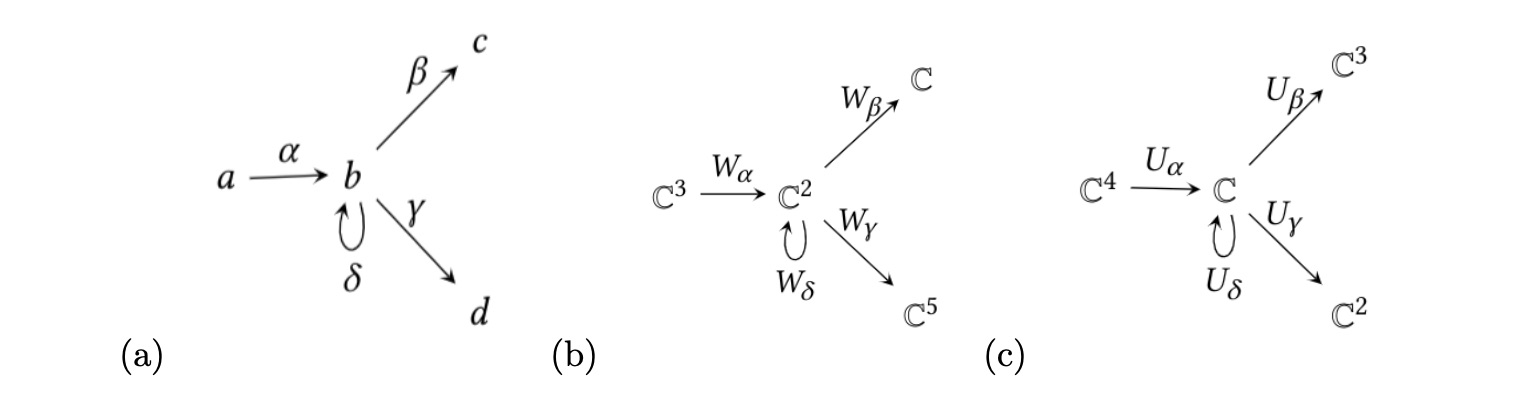
Figure 6: Additonal examples of quivers. (a): A quiver $Q$ with vertices $V=\{a,b,c,d\}$ and oriented edges $E=\{\alpha,\beta,\gamma,\delta\}$, (b) and (c): two quiver representations over $Q$. Adapted from Armenta & Jodoin (2021)

We now want to formulate a collection of quiver representations into a category in order to be able to apply a homological algebra framework. We define a category ${\rm Rep}(Q)$ where the objects are representations of $Q$. For any two representations $V$ and $W$ $Q=(Q_{0},Q_{1},h,t)$. We define a morphism $\phi:V\rightarrow W$ by attaching to every vertex $x\in Q_{0}$ a $\mathbb{C}$ linear map $\phi(x):V(x)\rightarrow W(x)$ such that for every $a\in Q_{1}$ the diagram

(16)

commutes, i.e., $\phi(ha)V(a)=W(a)\phi(ta)$.

Definition 4.3.

A path $p$ in a quiver $Q=(Q_{0},Q_{1},h,t)$ of length $l\geq 1$ is a sequence $p=a_{l}a_{l-1}\cdots a_{1}$ of arrows in $Q_{1}$ such that $ta_{i+1}=ha_{i}$ for $i=1,2,\ldots,l-1.$ We define $h(p)=hp=ha_{l}$ and $t(p)=tp=ta_{1}.$ For every $x\in Q_{0}$, we introduce a trivial path $e_{x}$ of length $0$. We define $he_{x}=te_{x}=x$.

Definition 4.4.

The path algebra $\mathbb{C}Q$ is a $\mathbb{C}$-algebra with a basis labeled by all paths in $Q$. We denote by $\langle p\rangle$ the element of $\mathbb{C}Q$ corresponding to the path $p$ in $Q$. The multiplication in $\mathbb{C}Q$ is given by

$$\langle p\rangle\cdot\langle q\rangle=\left\{\begin{array}[]{rcl}\langle pq\rangle&\mbox{if}&tp=hq,\\ \\ 0&\mbox{if}&tp\neq hq.\end{array}\right.$$ (20)

Here $pq$ denotes the concatenation of paths, and we use the conventions $pe_{x}=p$ if $tp=x$, and $e_{x}p=p$ if $hp=x$.

Proposition 4.5.

The categories $\textbf{Rep}(Q)$ and $\mathbb{C}Q$-mod are equivalent.

This result is proven as Proposition 1.5.4 in Derksen & Weyman (2017). It implies that every quiver representation, including network structures, can be interpreted as a module, an algebraic structure. The category of quiver representations, therefore, behaves similarly as the category of modules. In other words, $\textbf{Rep}(Q)$ can be shown to be indeed an Abelian category, so the constructions of homological algebra are available. Thus, we can use tools primarily from linear algebra and graph theory, to compute emergence as the algebraic structure arising from the interactions between quiver representations.

5 Computing the derived functors

In Section 3 we introduced how the cohomology object $L^{1}\Phi(A)$ or $R^{1}\Phi(A)$ is able to encode the emergence of system $A$ in a non-trivial way. In this section we discuss how it is computed, resulting in Proposition 5.3 that leads to a computational measure of emergence.

The first step is to find the projective/injective resolutions associated with a quiver representation. Let $Q=(Q_{0},Q_{1},h,t)$ be an acyclic quiver. We investigate the structure of projective and injective resolutions in $\textbf{Rep}(Q)$. For $x\in Q_{0}$, define $\mathbb{C}Q$-modules $P_{x}:=\mathbb{C}Qe_{x}$ and $I_{x}=(e_{x}\mathbb{C}Q)^{*}$, the dual space of $e_{x}\mathbb{C}Q$ defined as ${\rm Hom}(e_{x}\mathbb{C}Q,\mathbb{C})$. Here $\mathbb{C}Qe_{x}$ gives us the algebra whose basis is given by the paths starting from node $x$.

From Derksen & Weyman (2017), for representation $V$ in $\textbf{Rep}(Q)$ we have the projective resolution

(21)

where

$$f^{V}:\bigoplus\limits_{x\in Q_{0}}V(x)\otimes P_{x}\rightarrow V$$ (22)

is defined by

$$f^{V}(p\otimes v)=p\cdot v,$$ (23)

and

$$d^{V}:\bigoplus\limits_{a\in Q_{1}}V(ta)\otimes P_{ha}\rightarrow\bigoplus\limits_{x\in Q_{0}}V(x)\otimes P_{x}$$ (24)

is defined by

$$d^{V}(v\otimes p)=(a\cdot v)\otimes p-v\otimes ap.$$ (25)

And dually, for representation $W$ in $\textbf{Rep}(Q)$, the injective resolution is

(26)

where

$$f^{*}_{W}:\bigoplus\limits_{x\in Q_{0}}W(x)^{*}\otimes I_{x}^{*}\rightarrow W^{*}$$ (27)

is defined by

$$f^{*}_{W}(p\otimes w)=p\cdot w,$$ (28)

and

$$d^{*}_{W}:\bigoplus\limits_{a\in Q_{1}}W(ha)^{*}\otimes I_{ta}^{*}\rightarrow\bigoplus\limits_{x\in Q_{0}}W(x)^{*}\otimes I_{x}^{*}$$ (29)

is defined by

$$d^{*}_{W}(w\otimes p)=w\otimes ap-(a\cdot w)\otimes p.$$ (30)

Here the dual $W^{*}$ of a quiver representation $W$ in $\textbf{Rep}(Q)$ can be understood as a representation of the opposite quiver $Q^{op}$, obtained by reversing the direction of each arrow in $Q$.

Proposition 5.1.

The complexes represented by 21 and 26 are exact.

Proof.

This is proved in Derksen & Weyman (2017) Proposition 2.3.4. ∎

Following the definition of derived functors in Section 3, the left derived functor $L^{n}\Phi$ and the right derived functor $R^{n}\Phi$ can be computed from the following sequences, which are the image of the resolutions under the functor $\Phi$:

(31)

when $\Phi$ is right exact and

(32)

when $\Phi$ is left exact.

which yields

$$L^{0}\Phi(V) =H^{0}I^{\bullet}(V)=\Phi(V)$$ (33)

$$L^{1}\Phi(V) =H^{1}I^{\bullet}(V)=\ker\Phi d^{V}$$ (34)

when $\Phi$ is right exact and

$$R^{0}\Phi(W) =H^{0}I^{\bullet}(W)=\Phi(W)$$ (35)

$$R^{1}\Phi(W) =H^{1}I^{\bullet}(W)=\Phi(\bigoplus\limits_{a\in Q_{1}}I_{ta}\otimes W(ha))/{\rm Im}d_{W}$$ (36)

when $\Phi$ is left exact.

This means to find the emergence of a system, we need to solve equation (34) or (36).

Now we discuss our choice of functors $\Phi$. Given a class of functors $\{\Phi_{\delta}\}$, the goal is to find those that could sustains emergent effects, and especially those with stronger potentials for emergent effects. The class of functors $\{\Phi_{\delta}\}$ of interest will often neglect the partial structure of the system, which resembles information processing systems where some connections are neglected, a ubiquitous class in both natural and engineered systems.

In order to construct functors like this, and also satisfy one-side exact so that our previous theoretic framework, we assume the following structure to the vector spaces and their morphisms: for any representation $V$ in $\textbf{Rep}(Q)$, for each vector space $V(x)$, it is composed of an input space $V_{in}(x)$ and an output space $V_{out}(x)$, so that $V(x)=V_{in}(x)\oplus V_{out}(x)$. We study morphisms such that their restrictions at a node $f(x):V(x)\rightarrow W(x)$ satisfy $f(V(x))\subseteq W_{in}(x)$. The motivation is such that the arrows as information flows go from an output space into an input space. This can be formulated as filtered vector spaces. From an applied perspective, any network whose nodes have an input and output can be modeled as such a structure. And by removing $V_{in}(x)$ or $V_{out}(x)$, we are effectively removing edges going into/out of node $x$.

In this paper, we consider the following functors:

• $\Phi_{l}$, which maps $W_{out}(x)$ to zero for $x$ in a fixed set of nodes $N$, thus truncating edges coming from $W(x)$.

• $\Phi_{r}$, which maps $W_{in}(x)$ to zero for $x$ in a fixed set of nodes $N$, thus truncating edges coming into $W(x)$.

Proposition 5.2.

$\Phi_{l}$ is left exact and $\Phi_{r}$ is right exact.

Proof.

As proved in Rotman & Rotman (2009), a functor is left exact when it preserves kernel and right exact when it preserves cokernel. For $\Phi_{l}$, every morphism $f:W_{in}(x)\oplus W_{out}(x)\rightarrow V_{in}(x)$ is mapped to $W_{in}(x)\rightarrow V_{in}(x)$, which preserves injectiveness thus the kernel, so it is left-exact. For $\Phi_{r}$, every morphism $W_{in}(x)\oplus W_{out}(x)\rightarrow V_{in}(x)$ is mapped to $W_{out}(x)\rightarrow 0$, which preserves surjectiveness thus the cokernel. Hence it is right-exact. ∎

Now we give the following proposition that quantifies emergence of such a system:

Proposition 5.3.

The first left derived functor of $\Phi_{r}$ is

$$L^{1}\Phi_{r}(V)=\bigoplus_{a\in E}\Phi_{r}(V(ta))\otimes\Phi_{r}(P_{ha})$$ (37)

where $E$ is the set of edges being neglected by $\Phi_{r}$, $P_{ha}$ is the path algebra spanned by all paths from the head of edge $a$.

The higher left derived functors of $\Phi_{r}$ are trivial.

The first right derived functor of $\Phi_{l}$ is

$$R^{1}\Phi_{l}(W)=\bigoplus_{a\in E}\Phi_{l}(W(ha))\otimes\Phi_{l}(I_{ta})$$ (38)

where $E$ is the set of edges being neglected by $\Phi_{l}$, $I_{ha}$ is the path algebra spanned by all paths to the tail of edge $a$.

The higher right derived functors of $\Phi_{l}$ are trivial.

Proof.

First, since the injective and projective resolutions in the category of quiver representations has length $2$, we can see that all higher derived functors will vanish.

We already proved in the previous proposition that $\Phi_{r}$ is right exact, so we compute the zeroth left derived functor is itself (see, for example, Rotman & Rotman (2009)). Now we compute the first left derived functor $L^{1}\Phi_{r}$. From (34), $L^{1}\Phi_{r}=\ker\Phi_{r}d^{V}$, where $d^{V}$ is defined in (24). Now if an edge $a$ is neglected as a consequence of $W_{in}(x)$ mapped to zero, then for any $v\in V(ta)$ and $p\in P_{ha}$, we have$(a\cdot v)\otimes p=v\otimes ap=0$, hence $\Phi(V(ta)\otimes P_{ha}\subseteq\ker\Phi_{r}d^{V}$. If $a$ is preserved under $\Phi_{r}$, then $\Phi_{r}(V(ta)\otimes P_{ha}$ will be non-zero thus not contribute to $\ker\Phi_{r}d^{V}$.

Now for the left exact functor $\Phi_{l}$, by definition its first right derived functor $R^{1}\Phi_{l}$ is computed as $\Phi_{l}(\bigotimes_{a\in Q_{1}}I_{ta}\otimes W(ha))/\text{Im}d_{W}$ from the injective resolution, and since the injective resolution is obtained from the projective resolution by taking the dual, we have $R^{1}\Phi_{l}(W)=L^{1}\Phi_{r}(W^{*})$ where $W^{*}$ the dual of $W$ is the opposite quiver representation of $W$ obtained by reversing the direction of all edges. Under this choice, $W^{*}(ha)=W(ta)$, and $P^{*}(ta)=I_{ta}$.

∎

This proposition informs us that under the choice of the functor which kills the input/output space of some nodes in the network, emergence as $L^{1}\Phi(A)$ or $R^{1}\Phi(A)$ encodes the edges thus being neglected. It consists of the direct product of path algebras, spanned by some paths that go through the edges being neglected. So we can interpret the algebraic structure we computed as the part of the quiver representation that is impacted by the functor or neglected by the partial observations, which is responsible for the emergent structure/ pattern. It is also worth pointing out that, we can generalize this proposition to the situation where the functor is reducing the dimensionality of $W_{in}$ or $W_{out}$ instead of mapping it to zero. This requires us to introduce more grade/filter structure to the vector spaces, and this will be discussed in our following work that studies how local structures impact the global emergence.

6 A Numerical Measure of Emergence

In proposition 5.3, the emergence of system $A$ is encoded as the cohomology $L^{1}\Phi(A)$ or $R^{1}\Phi(A)$. It will be torsion-free, hence the information is encoded in its dimension, which can be regarded as a numerical measure to evaluate the emergence of a system.

$$\dim L^{1}\Phi_{r}(A) =\dim\bigoplus_{a\in E}\Phi_{r}(V(ta))\otimes\Phi_{r}(P_{ha})$$

$$=\sum_{a\in E}\dim\Phi_{r}(V(ta))\times\dim\Phi_{r}(P_{ha})$$ (39)

Similarly,

$$\dim R^{1}\Phi_{l}(A) =\dim\bigoplus_{a\in E}\Phi_{l}(W(ha))\otimes\Phi_{l}(I_{ta})$$

$$=\sum_{a\in E}\dim\Phi_{l}(W(ha))\times\dim\Phi_{l}(I_{ta})$$ (40)

In order to understand this computational measure, it is important to understand the path algebra $P_{x}$ here. $P_{x}$ can be regarded as a quiver representation where the vector space associated with each node has the same dimension as the number of path from $x$ to this node Derksen & Weyman (2017). So we can understand that the dimension of an algebra $P_{x}$ is the same as the number of paths originating from $x$. From this we can also see that $L^{1}\Phi(A)$ or $R^{1}\Phi(A)$ can be regarded as a quiver representation as well.

Note that here we are summing over the dimension of vector spaces associated with all the nodes in the quiver representations corresponding to $L^{1}\Phi_{r}(A)$ or $R^{1}\Phi_{l}(A)$ in order to have a global measure of emergence. By evaluating first the dimension of each vector space, we can find the contribution of each node to the global emergence, which is an important feature of our framework of emergence. It addressed the issue we discussed in the introduction part of this paper.

Let us discuss this measure when we come down to graph theory. A graph can be regarded as a quiver representation where the input and output vector space associated with each node is $1$ dimensional. This kind of quiver representation is considered in, for example, (Armenta & Jodoin, 2021; Ganev & Walters, 2022). Now based on equations (39) and (40) we have a measure of emergence when we pass from a graph $G$ to its subgraph $H$ by neglecting the edges coming out of nodes in $G\setminus H$:

$$\text{Emergence}(G,H) =\sum_{x\in G\setminus H}\#\text{paths in $G$ from $G\setminus H$ to $H$}.$$ (41)

Note that this result assumes the functor $\Phi$ as truncating nodes in $G\setminus H$. The measure of emergence here could have different forms under other choices of $\Phi$, which will be explored in our next work. This result quantifies emergence as counting the number of paths generated from the nodes being truncated by the partial observation. It provides us with a numerical measure of emergence that is based on the local network structure, which is the path originating from each node in $G\setminus H$. Applying Proposition 5.3, when the functor $\Phi$ neglects more edges, it implies stronger emergence. This conceptually agrees with other existing measures. For example in Gershenson & Fernández (2012) emergence is defined as the information loss

$$E=\frac{I_{\text{out}}}{I_{\text{in}}}$$ (42)

where $I_{\text{in}}$ is the ”input information” and $I_{\text{out}}$ is the ”output information”, which can be seen as $I_{\text{in}}$ transformed by a computational process. Gershenson & Fernández (2012) simulated random Boolean networks with different connectivity $K$ and found that the loss of emergence increases with $K$. Larger $K$ corresponds to fewer neglected edges, which is equivalent to smaller $L^{1}\Phi(A)$. This means that $\Phi(s_{1}\vee s_{2})$ is closer to $\Phi(s_{1})\vee\Phi(s_{2})$, which implies less information loss and greater $E$.

Importantly, our measure associates the the global property of emergence with specific nodes and edges. Compared to information-theoretic approaches, our measure provides mechanistic insights into the subsystems responsible for observed emergent phenomena. We plan to study this in detail in future work.

In summary, the approach we developed for evaluating the emergent effect of a network system $A$ can be sketched as follows:

1. Encode the system $A$ as a quiver representation, i.e., a network where each node is associated with a vector space, and each edge a linear map.

2. Realize the partial observation as a functor $\Phi$ which kills the input/output edges of chosen nodes, for example, those that are inactive in a computational process.

3. Use Proposition 5.3 or Equation (41) to obtain an algebraic/numerical evaluation of emergence.

We have developed a measure for emergence, and now we demonstrate numerically that the measure offers computational insights for network systems, modeled as quiver representations. We consider random Boolean network (see, Kauffman, 1969; Gershenson, 2004), a type of mathematical model used to represent genetic regulatory networks and study their dynamics. These networks consist of nodes (or vertices) and directed edges (or links). Each node in the network can be in one of two states, typically represented as 0 or 1 (or ”off” and ”on”). Random Boolean network can be characterized by the connectivity parameter $K$, where each node in the network receives input from $K$ nodes.

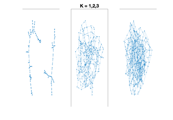
Figure 7: Examples of random Boolean network for $K=1,2,3$.

Random Boolean network can be regarded as a generalization of cellular automata Gershenson (2004), and has been used as models to study emergent behavior, especially in the context of biological and complex systems(see, Kauffman, 1993; Gershenson, 2003). In Gershenson & Fernández (2012), random Boolean networks of different connnectivities has been simulated, and the information loss as in (42) has been proposed as a measure of emergence, where $I_{out}$ is the Shannon information measured at the end state of the network and $I_{in}$ is the Shannon information measured at the initial state of the network. To compare our measure of emergence with this measure, we run our simulation on networks with a range of connectivities $K$ where the edges and activation functions are randomly generated. We measure emergence of such random Boolean networks by regarding the functor $\Phi_{l}$ as the one that sends a fully connected network $G$ to subnetwork $H$ which remains active during the network dynamics. A node is considered inactive here when it comes into state $1$ in less than $5\%$ of the time after the network dynamics reaches steady state. We consider the quiver representation for each network that has dimension $1$ for the input and output space of each node, and as discussed above, and emergence reflects the number of paths being ”impacted” by the functor. We compared our measure of emergence with the information-theoretic measure of emergence as information loss in Figure 8.

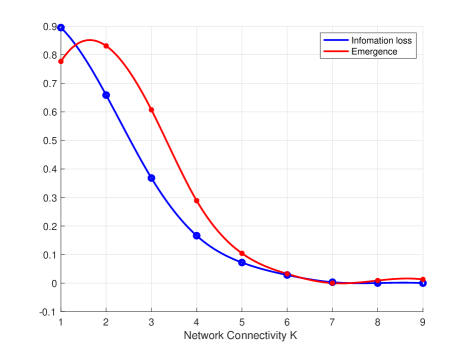
Figure 8: Comparison of emergence and information loss at different network connectivity $K$.

In our computation, we averaged over the random network ensemble of size $1000$. The network has $10$ nodes in total, when $K=9$ the network is fully connected. The initial state of the network is randomized and the probability for each node to be active is $1/2$. We simulate the network for $200$ time steps and it is observed that the network dynamics reach steady state in fewer than $100$ time steps. The emergence is normalized by the maximum and minimum value among all possible value of $K$. The normalized information loss is computed here as

$$E^{\prime}=1-\frac{I_{K}}{I}$$ (43)

where $I_{K}$ is the Shannon information of the network with connectivity $K$ when it reaches steady state and $I$ is the Shannon information of the fully connected network when it reaches steady state. If we regard the computational process as follows: the input is the entropy of the fully connected network and the output is the entropy of the $K$ connected network, then $I_{K}/I$ is interpreted as $E$ in Equation (42) in this way.

From the simulation, we can see that our measure of emergence correlates with information loss, as a way to measure emergence on the random Boolean networks of different connectivity. The difference here is emergence seems to favor $K=2$ over $K=1$, contrary to information loss. We think there is a connection between our measure of emergence and information loss, although it is not proved at the current stage. As an interpretation, the functor $\Phi$ we choose sends the fully connected network $G$ to the subnetwork $H$ of active nodes. Since the active nodes are given by the steady state of network dynamics, the functor ties the steady state of some connectivity $K$ network to the steady state of the fully connected network. Emergence in this context thus captures the difference between the steady states, and more generally the impact connectivity $K$ has on network dynamics.

We plot emergence together with the percentage of inactive nodes in Figure 9. We can observe that emergence largely correlates with the percentage of inactive nodes in a random Boolean network. Although emergence is dependent on the specific positions of the inactive nodes, we can still see a correlation between emergence and the average number of inactive nodes. This agrees with our intuition in Section 2 and equation (41).

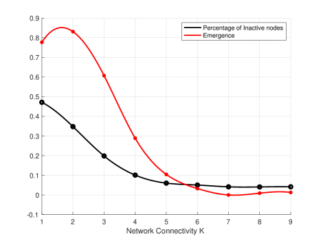
Figure 9: Emergence and the percentage of inactive nodes at different network connectivity $K$.

7 Discussion and Conclusion

We have established a framework that quantifies the emergence of systems based on their structural information, modeled by quiver representations, and we build a computational measure that quantifies the emergence of systems realized as the mapping between networks where only partial nodes and edges are being preserved, which can be used to model a large variety of systems characterized by the information flow on the network. Other kinds of information flow, for example, those involves coarse-graining, can also be studied by constructing the functors that capture the information flow and compute their derived functors. The emergence is formulated in homological algebra as the ”loss of exactness”, the loss of the algebraic property when a sequence of subsystems modeling interactions is mapped to their partial observations. We showed that our measure correlates with the information-theoretic measure of emergence on random Boolean networks. One important feature of our measure is, as discussed in Section 6, it offers a way to study the contribution of each node to emergence, which is a global property. This could allow us to track the contribution of each node to emergence in a dynamic process, which can help detect the mechanisms of emergence.

Although this framework is algebraic in its nature, we have shown that it can lead to computational measures that are applicable to real-world systems. The key is to choose the appropriate categories and functors to work on that have both relatively good algebraic properties and strong descriptive power to real-world systems. For example, if researchers aim at studying the emergent abilities of machine learning systems, the functor could be the one that ties the systems (for example, parts of the neural network architecture) to its performance, for example, on some data set and downstream tasks. The fundamental constraints within the framework is that System and Phenome have to be Abelian categories (or the extension of it that allows the discussion of homological algebra) and the functor $\Phi$ has to be exact at one side (either left exact or right exact). The first constraint is tackled by considering the category of quiver representations, which is Abelian, with nice homological algebra properties and can encode network systems. The second constraint is tackled by breaking the nodes into input space and output space, and the functor that truncates only on one of the spaces can often be one-side exact. By these constructions we allow our framework applicable to a large class of real-world systems. We also leave a lot of mathematical quests to be investigated later, for example, when the System category is no longer an Abelian category, we can either lift it to Abelian category, as discussed in Adam (2017), or develop homological algebra in a non-Abelian case. It is in general an intriguing task to find new categories to work on to yield insights in network science or other disciplines in science and engineering. Also, the mathematical theory of quiver representations is itself a massive topic, with growing applications to physical systems and network theory, which will be an interesting exploration as well to combine with the homological algebra approach.

From a modeling and computational perspective, our work provides an approach to quantify the emergence of systems as networks, or more generally, quiver representations. It can capture not only the connectivity patterns of the components, but also the structures and dynamics at each node and edge. Within the framework of quiver representations, the mappings between vector spaces need to be linear maps, which render the framework hard to capture the non-linearity, like the activation function in the artificial and biological neural networks. But still, quiver representation can be applied to model data and its network structures, so our work can be applied to the phase space of the dynamics, like the spike train data and cellular automata. Also, there has been theoretical development to model neural network based on quiver representations (see Jeffreys & Lau, 2022; Armenta & Jodoin, 2021). Additionally, the computation of emergence based on networks or quiver representations would often involve counting the number of certain paths in the network, which would require searching algorithms that are time-consuming if the network is large. We call for new approximation schemes and algorithms that evaluate emergence in a cheaper way.

To our knowledge, this is the first work that computationally evaluates emergent effects in a system and its constituent parts, thus opening up exciting new research avenues that lead to an understanding of emergence mechanisms of systems of interest, which could potentially apply to, for example, the optimization of network architecture that encourages or discourages emergence so as to achieve better performance in deep learning tasks, and the study of the cause of neuro-deficiencies from the activity and morphology of neurons. In future work, we will apply this framework to the study of the emergent effects of biological and machine learning systems. For networks in these fields, the nodes and edges often have intricate internal structures that traditional models are not able to capture. We will model these kinds of networks as quiver representations or other mathematical structures. There are topics in these fields that are related to emergence, like phase transition, symmetry breaking and generalizability of artificial neural networks, and we aim at establishing the connections between emergence and these concepts as well.

Acknowledgments

The authors would like to thank Dr. Elie Adam for the extensive conversations on the theoretical foundation of this work. This work was supported by unrestricted research funds to the Center for Engineered Natural Intelligence (CENI) at the University of California San Diego.

References

- (1)
- Anderson (1972) Anderson, P. More is different: broken symmetry and the nature of the hierarchical structure of science.. Science. 177, 393-396 (1972).
- Kalantari et al. (2020) Kalantari, S., Nazemi, E. & Masoumi, B. Emergence phenomena in self-organizing systems: a systematic literature review of concepts, researches, and future prospects. Journal Of Organizational Computing And Electronic Commerce. 30, 224-265 (2020).
- Post & Weiss (1997) Post, R. & Weiss, S. Emergent properties of neural systems: How focal molecular neurobiological alterations can affect behavior. Development And Psychopathology. 9, 907-929 (1997).
- O’Connor (2020) O’Connor, T. Emergent properties. (2020).
- Forrest (1990) Forrest, S. Emergent computation: Self-organizing, collective, and cooperative phenomena in natural and artificial computing networks: Introduction to the proceedings of the ninth annual cnls conference. Physica D: Nonlinear Phenomena. 42, 1-11 (1990).
- Wei et al. (2022) Wei, J., Tay, Y., Bommasani, R., Raffel, C., Zoph, B., Borgeaud, S., Yogatama, D., Bosma, M., Zhou, D., Metzler, D. & Others Emergent abilities of large language models. ArXiv Preprint ArXiv:2206.07682. (2022)
- Mohammed & Kora (2023) Mohammed, A. & Kora, R. A comprehensive review on ensemble deep learning: Opportunities and challenges. Journal Of King Saud University-Computer And Information Sciences. (2023)
- Teehan et al. (2022) Teehan, R., Clinciu, M., Serikov, O., Szczechla, E., Seelam, N., Mirkin, S. & Gokaslan, A. Emergent structures and training dynamics in large language models. Proceedings Of BigScience Episode 5–Workshop On Challenges & Perspectives In Creating Large Language Models. pp. 146-159 (2022)
- Barabasi & Oltvai (2004) Barabasi, A. & Oltvai, Z. Network biology: understanding the cell’s functional organization. Nature Reviews Genetics. 5, 101-113 (2004)
- Crutchfield (1994) Crutchfield, J. The calculi of emergence: computation, dynamics and induction. Physica D: Nonlinear Phenomena. 75, 11-54 (1994)
- Bar-Yam (2004) Bar-Yam, Y. A mathematical theory of strong emergence using multiscale variety. Complexity. 9, 15-24 (2004)
- Gershenson & Fernández (2012) Gershenson, C. & Fernández, N. Complexity and information: Measuring emergence, self-organization, and homeostasis at multiple scales. Complexity. 18, 29-44 (2012)
- Correa (2020) Correa, J. Metrics of emergence, self-organization, and complexity for EWOM research. Frontiers In Physics. 8 pp. 35 (2020)
- Varley & Hoel (2022) Varley, T. & Hoel, E. Emergence as the conversion of information: A unifying theory. Philosophical Transactions Of The Royal Society A. 380, 20210150 (2022)
- Green (2023) Green, D. Emergence in complex networks of simple agents. Journal Of Economic Interaction And Coordination. pp. 1-44 (2023)
- Mediano et al. (2022) Mediano, P., Rosas, F., Luppi, A., Jensen, H., Seth, A., Barrett, A., Carhart-Harris, R. & Bor, D. Greater than the parts: a review of the information decomposition approach to causal emergence. Philosophical Transactions Of The Royal Society A. 380, 20210246 (2022)
- Adam (2017) Adam, E. Systems, generativity and interactional effects. (Massachusetts Institute of Technology,2017)
- Mac Lane (2013) Mac Lane, S. Categories for the working mathematician. (Springer Science & Business Media,2013)
- Freyd (1964) Freyd, P. Abelian categories. (Harper & Row New York,1964)
- Derksen & Weyman (2005) Derksen, H. & Weyman, J. Quiver representations. Notices Of The AMS. 52, 200-206 (2005)
- Derksen & Weyman (2017) Derksen, H. & Weyman, J. An introduction to quiver representations. (American Mathematical Soc.,2017)
- Schiffler, (2014) Schiffler, R. Quiver representations. (Springer,2014)
- Cartan & Eilenberg (1999) Cartan, H. & Eilenberg, S. Homological algebra. (Princeton university press,1999)
- Gelfand & Manin (2013) Gelfand, S. & Manin, Y. Methods of homological algebra. (Springer Science & Business Media,2013)
- Rotman & Rotman (2009) Rotman, J. & Rotman, J. An introduction to homological algebra. (Springer,2009)
- Silva (2019) Silva, G. The effect of signaling latencies and node refractory states on the dynamics of networks. Neural Computation. 31, 2492-2522 (2019)
- Puppo et al. (2018) Puppo, F., George, V. & Silva, G. An optimized structure-function design principle underlies efficient signaling dynamics in neurons. Scientific Reports. 8, 10460 (2018)
- George et al. (2022) George, V., Morar, V. & Silva, G. A Computational Model for Storing Memories in the Synaptic Structures of the Brain. BioRxiv. pp. 2022-10 (2022)
- Armenta & Jodoin (2021) Armenta, M. & Jodoin, P. The representation theory of neural networks. Mathematics. 9, 3216 (2021)
- Silva & others (2020) Silva, G. & Others A category theory approach using preradicals to model information flows in networks. ArXiv Preprint ArXiv:2012.02886. (2020)
- Silva & others (2021) Silva, G. & Others Information entropy re-defined in a category theory context using preradicals. ArXiv Preprint ArXiv:2112.06034. (2021)
- Silva (2011) Silva, G. The need for the emergence of mathematical neuroscience: beyond computation and simulation. Frontiers In Computational Neuroscience. 5 pp. 51 (2011)
- (34) Buibas, M. & Silva, G. A framework for simulating and estimating the state and functional topology of complex dynamic geometric networks. Neural Computation. 23, 183-214 (2011)
- Snooks & others (2008) Snooks, G. & Others A general theory of complex living systems: Exploring the demand side of dynamics. Complexity. 13, 12-20 (2008)
- Rosen (1958a) Rosen, R. A relational theory of biological systems. The Bulletin Of Mathematical Biophysics. 20 pp. 245-260 (1958)
- Rosen (1958b) Rosen, R. The representation of biological systems from the standpoint of the theory of categories. The Bulletin Of Mathematical Biophysics. 20 pp. 317-341 (1958)
- Hoff et al. (2004) Hoff, M., Roggia, K. & Menezes, P. Composition of transformations: A framework for systems with dynamic topology. International Journal Of Computing Anticipatory Systems. 14 pp. 259-270 (2004)
- Peak et al. (2004) Peak, D., West, J., Messinger, S. & Mott, K. Evidence for complex, collective dynamics and emergent, distributed computation in plants. Proceedings Of The National Academy Of Sciences. 101, 918-922 (2004)
- Gadioli La Guardia & Jeferson Miranda (2018) Gadioli La Guardia, G. & Jeferson Miranda, P. On a categoriacal theory for emergence. ArXiv E-prints. pp. arXiv-1810 (2018)
- Bassett & Sporns (2017) Bassett, D. & Sporns, O. Network neuroscience. Nature Neuroscience. 20, 353-364 (2017)
- Bassett et al. (2018) Bassett, D., Zurn, P. & Gold, J. On the nature and use of models in network neuroscience. Nature Reviews Neuroscience. 19, 566-578 (2018)
- Northoff et al. (2019) Northoff, G., Tsuchiya, N. & Saigo, H. Mathematics and the brain: a category theoretical approach to go beyond the neural correlates of consciousness. Entropy. 21, 1234 (2019)
- Bradley (2018) Bradley, T. What is applied category theory?. ArXiv Preprint ArXiv:1809.05923. (2018)
- Fong & Spivak (2018) Fong, B. & Spivak, D. Seven sketches in compositionality: An invitation to applied category theory. ArXiv Preprint ArXiv:1803.05316. (2018)
- Parada-Mayorga et al. (2020) Parada-Mayorga, A., Riess, H., Ribeiro, A. & Ghrist, R. Quiver signal processing (qsp). ArXiv Preprint ArXiv:2010.11525. (2020)
- Ganev & Walters (2022) Ganev, I. & Walters, R. Quiver neural networks. ArXiv Preprint ArXiv:2207.12773. (2022)
- Jeffreys & Lau (2022) Jeffreys, G. & Lau, S. Kähler Geometry of Framed Quiver Moduli and Machine Learning. Foundations Of Computational Mathematics. pp. 1-59 (2022)
- Kirillov Jr (2016) Kirillov Jr, A. Quiver representations and quiver varieties. (American Mathematical Soc.,2016)
- Kauffman (1969) Kauffman, S. Metabolic stability and epigenesis in randomly constructed genetic nets. Journal Of Theoretical Biology. 22, 437-467 (1969)
- Gershenson (2004) Gershenson, C. Introduction to random Boolean networks. ArXiv Preprint Nlin/0408006. (2004)
- Kauffman (1993) Kauffman, S. The origins of order: Self-organization and selection in evolution. (Oxford University Press, USA,1993)
- Gershenson (2003) Gershenson, C. Classification of random Boolean networks. Artificial Life VIII, Proceedings Of The Eighth International Conference On Artificial Life. pp. 1-8 (2003)