Diffusion-driven flows in a non-linear stratified fluid layer

Abstract

Diffusion-driven flow is a boundary layer flow arising from the interplay of gravity and diffusion in density-stratified fluids when a gravitational field is non-parallel to an impermeable solid boundary. This study investigates diffusion-driven flow within a nonlinearly density-stratified fluid confined between two tilted parallel walls. We introduce a novel asymptotic expansion inspired by the center manifold theory, where quantities are expanded in terms of derivatives of the cross-sectional averaged density field. This technique provides accurate approximations for velocity, density, and pressure fields. Furthermore, we derive an evolution equation describing the cross-sectional averaged density field. This equation takes the form of the traditional diffusion equation but replaces the constant diffusion coefficient with a positive-definite function dependent on the solution’s derivative. Numerical simulations validate the accuracy of our approximations. Our investigation of the effective equation reveals that the density profile depends on a non-dimensional parameter denoted as $\gamma$ which is related to the flow strength. In the large $\gamma$ limit, the system emulates a diffusion process with an augmented diffusion coefficient of $1+\cot^{2}\theta$, where $\theta$ signifies the inclination angle of the channel domain. This parameter regime is where diffusion-driven flow exhibits its strongest mixing ability. Conversely, in the small $\gamma$ regime, the density field behaves akin to pure diffusion with distorted isopycnals. Lastly, we show that the classical thin film equation aligns with the results obtained using the novel expansion in the small $\gamma$ regime but fails to accurately describe the dynamics of the density field for large $\gamma$.

1 Introduction

The density of a fluid is influenced by several factors, including temperature, the concentration of solute, and pressure profiles. Typically, these factors lead to a non-uniform distribution of density in the fluid. Density stratified fluids are commonly found in various natural environments, such as lakes, oceans, the Earth’s atmosphere, making them a subject of great interest in numerous research endeavors (Linden (1979); Cenedese & Adduce (2008); Magnaudet & Mercier (2020); Camassa et al. (2022); More & Ardekani (2023)). In the context of density-stratified fluids, achieving hydrostatic equilibrium is contingent upon aligning the density gradients with the direction of gravitational force. In scenarios involving impermeable boundaries and the modeling of diffusive stratifying scalars, the no-flux boundary condition is employed. This condition necessitates that density gradient is orthogonal to the boundary’s normal vector, and thus, the density gradient and boundary direction cannot simultaneously coincide if the impermeable boundary deviates from the gravitational direction. The disruption of hydrostatic equilibrium results in the emergence of a boundary layer flow, a phenomenon termed diffusion-driven flows in the field of physics (Phillips (1970); Wunsch (1970)), or mountain and valley (katabatic or anabatic) winds (Prandtl et al. (1942); Oerlemans & Grisogono (2002)) in meteorology.

The phenomenon of diffusion-driven flow has garnered significant attention across various fields. Firstly, in the context of oceanography, the presence of salt in seawater leads to density stratification. The sloping boundaries of the ocean induce a mean upwelling velocity along the walls to satisfy the no-flux condition. This upwelling flow plays a crucial role in facilitating the vertical exchange of oceanic properties (see, for example, Phillips (1970); Wunsch (1970); Dell & Pratt (2015); Drake et al. (2020); Holmes et al. (2019)). Secondly, fluids confined within long, narrow fissures can also exhibit density stratification. This stratification can result from non-uniform concentration distributions of stratifying scalars or vertical temperature gradients. For example, Earth’s geothermal gradient induces convective flows that lead to significant solute dispersion on geological timescales (Woods & Linz (1992); Shaughnessy & Van Gilder (1995); Heitz et al. (2005)). Thirdly, when a wedge-shaped object is immersed in a stratified fluid, the resulting diffusion-driven flow can propel the object forward (as observed in research like Mercier et al. (2014); Allshouse et al. (2010)). The flows generated by such immersed wedge-shaped objects have been further investigated in various contexts (Chashechkin & Mitkin (2004); Zagumennyi & Dimitrieva (2016); Levitsky et al. (2019); Dimitrieva (2019); Chashechkin (2018)). Fourthly, diffusion-driven flow is one of the mechanisms that induce particle attraction and self-assembly in stratified fluids (Camassa et al. (2019); Thomas & Camassa (2023)). Fifthly, it has been demonstrated that this type of flow can be employed to measure the molecular diffusivity of stratifying scalars (Allshouse (2010)). Sixthly, flows induced by the presence of insulating sloping boundaries play an important role in the layer formation in double-diffusive systems (Linden & Weber (1977)).

Despite the significant findings in this field, there are two points that have not been adequately addressed in the existing literature. Firstly, most existing theories primarily pertain to linearly stratified fluids, and there is a scarcity of theoretical investigations into diffusion-driven flow in nonlinearly stratified fluids. Nonlinearly stratified fluids are more prevalent in various natural environments, making theoretical analysis in this context highly applicable. Secondly, there can exist two different type of scalars in the fluid: the concentration of the stratifying scalar and the passive scalar. The stratifying scalar causes non-uniform density distributions in the fluid and drives diffusion-driven flow. In contrast, the passive scalar represents the concentration of a different solute (in some cases, the temperature field) that doesn’t contribute to density variation but is instead passively advected by the fluid flow. It is well-established that fluid flow enhances solute mixing in the fluid ( Lin et al. (2011); Thiffeault (2012); Aref et al. (2017)). Many studies focus on how diffusion-driven flow enhances the dispersion of a passive scalar (Woods & Linz (1992); Ding & McLaughlin (2023)) and the corresponding analysis for the stratifying scalar are rare. Experiments, such as the one documented in (Ding (2022)), illustrate that the dispersion of the stratifying scalar in a tilting capillary pipe exhibits a higher dispersion rate compared to a vertically oriented pipe. This qualitative demonstration highlights the role of diffusion-driven enhancement at micro-scales. At diffusion timescales, the concentration of a diffusing passive scalar under the advection of shear flows can be described by an effective diffusion equation with an effective diffusion coefficient (Taylor (1953); Aris (1956)). Consequently, it is of interest to establish the evolution equation for the concentration of the stratifying scalar. This would enable us to quantitatively describe how diffusion-driven flow enhances the spreading rate of the stratifying scalar.

To address these research gaps, this paper delves into the study of an incompressible viscous density stratified fluid layer confined between two infinitely parallel walls. Investigating this fundamental domain geometry can enhance our comprehension of more intricate shapes found in real-world scenarios, such as rock fissures and capillary pipes. Furthermore, it provides a versatile framework for comprehending fluid dynamics within confined spaces, which holds substantial practical significance.

Our primary objectives are to derive approximations for the velocity field and density field and to determine the equation governing the dynamics of the fluid density field at diffusion time scales. One conventional approach, such as thin film approximation, involves introducing a small parameter and utilizing power series expansions for all relevant quantities with respect to this parameter. However, we demonstrate that results obtained through thin film approximation are only valid within specific parameter ranges and do not provide uniformly accurate approximations across all parameters. To obtain more approximations that accurately describe density dynamics across a wider parameter range, we adopt an alternative expansion method inspired by center manifold theory (Mercer & Roberts (1990); Roberts (1996); Ding & McLaughlin (2022a)). In this alternative approach, we assume that the density field varies slowly in the longitudinal direction of the channel. Then all quantities are represented in terms of derivatives of the averaged density field. This innovative approach enhances our ability to achieve accuracy in a broader range of flow scenarios.

This paper is organized as follows: In Section 2, we formulate the governing equations for diffusion-driven flow and outline the procedure for non-dimensionalization. Section 3 introduces a novel asymptotic expansion technique for the velocity, density, and pressure fields. Using this novel approach, we derive the leading-order approximation for the velocity field and establish the evolution equation for the cross-sectional averaged density field, referred to as the effective equation in subsequent sections. In Section 3.3, we conduct numerical simulations of the full governing equations to demonstrate the validity of the asymptotic approximations. Section 4 delves deeper into the properties of the effective equation, providing a more comprehensive understanding of its behavior in various scenarios. Section 5 documents the results obtained using the thin film approximation and compares them with the expansion proposed in Section 3. Finally, in Section 6, we summarize our findings and explore potential avenues for future research.

2 Governing equation and nondimensionalization

This section summarizes the mathematical formulation of the problem and documents the nondimensionalization procedure for the governing equation.

2.1 Governing equation

Figure 1 sketches two coordinate systems for a tilted parallel-plate channel domain with a inclination angle $\theta$ which satisfies $0\leq\theta\leq\frac{\pi}{2}$. In this setup, $x_{3}$-direction is parallel to the direction of gravity, $y_{1}$-direction is the longitudinal direction of the channel. $\Omega=\left\{y_{3}|y_{3}\in[0,L]\right\}$ is the cross-section of the channel. The relation between the lab frame coordinates $(x_{1},x_{2},x_{3})$ and the coordinates $(y_{1},y_{2},y_{3})$ is

$$\begin{bmatrix}y_{1}\\ y_{3}\\ \end{bmatrix} =\begin{bmatrix}\cos\theta&\sin\theta\\ -\sin\theta&\cos\theta\\ \end{bmatrix}\begin{bmatrix}x_{1}\\ x_{3}\\ \end{bmatrix},\quad y_{2}=x_{2}.$$ (1)

In the $(y_{1},y_{2},y_{3})$ coordinate system, gravity acts along the direction $(-\sin\theta,0,-\cos\theta)$. The channel can either extend infinitely with or have finite length. Experimental methods described in (Allshouse (2010); Heitz et al. (2005)) provide feasible setups for this study. Another promising experimental configuration involves using temperature-stratified liquid gallium (Braunsfurth et al. (1997)).

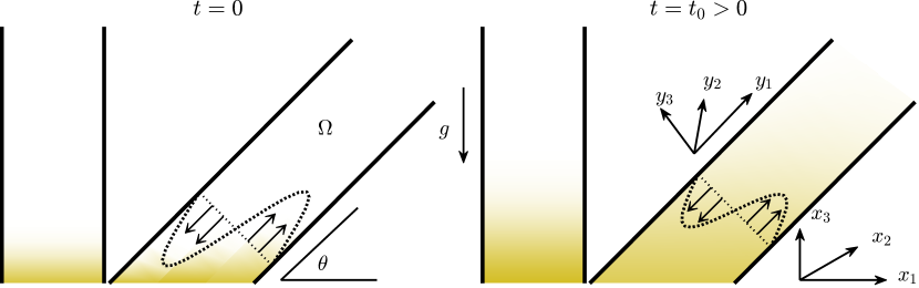
Figure 1: This schematic illustrates the setup for the diffusion-driven flow problem. Tilted impermeable boundaries induce the diffusion driven flow, while there is no flow in the vertically oriented channel. Pure molecular diffusion governs the scalar distribution in the latter case. As depicted in the left panel, at $t=0$, the concentration profiles are approximately the same in both channels. However, as time progresses, the dispersion of the scalar becomes more pronounced in the tilted channel compared to the vertically oriented one. In addition, the flow strength decrees as the density gradient decrees.

We assume the fluid density linearly depends on the concentration of the stratifying scalar. For example, the density of sodium chloride solution increases linearly as the concentration of the sodium chloride increases or temperature decreases (Hall (1924); Abaid et al. (2004)). Therefore, the density field $\rho$ and the fluid flow $\mathbf{u}=(u_{1},u_{2},u_{3})$ satisfies the incompressible Navier-Stokes equation,

$$\rho\left(\partial_{t}u_{i}+\mathbf{u}\cdot\nabla u_{i}\right)=\mu\Delta u_{i}-\partial_{x_{i}}p-\rho g\delta_{i3},\quad\left.u_{i}\right|_{\mathbf{x}\in\partial\Omega}=0,\quad i=1,2,3,$$ (2)

$$\nabla\cdot\mathbf{u}=0,\quad\partial_{t}\rho+\mathbf{u}\cdot\nabla\rho=\kappa\Delta\rho,\quad\left.\partial_{\mathbf{n}}\rho\right|_{\mathbf{x}\in\partial\Omega}=0,\quad\left.\rho\right|_{t=0}=\rho_{I}(\mathbf{x}).$$

where $\mathbf{n}$ is the outward normal vector of the boundary, $\delta_{ij}$ is the Kronecker delta, $g$ (cm/s²) is the acceleration of gravity, $\Gamma$ $(\text{gram}\cdot\text{cm}^{-4})$ is the density gradient, $\mu$ (gram$\cdot\text{cm}^{-1}\cdot\text{s}^{-1})$ is the dynamic viscosity, $p$ (gram$\cdot\text{cm}^{-1}\cdot\text{s}^{-2})$ is the pressure and $\kappa$ (cm${}^{2}/$s) is the molecular diffusivity of the stratified scalar.

It is convenient to consider the problem in $(y_{1},y_{2},y_{3})$ coordinate system. We denote $v_{i}$ as the velocity component along the $y_{i}$-direction. Since the initial condition and the boundary condition are independent of $y_{2}$, equation(2) reduces to a two-dimensional problem

$$\rho\left(\partial_{t}v_{1}+v_{1}\partial_{y_{1}}v_{1}+v_{3}\partial_{y_{3}}v_{1}\right)=\mu\Delta v_{1}-\partial_{y_{1}}p-\sin\theta g\rho,$$ (3)

$$\rho\left(\partial_{t}v_{3}+v_{1}\partial_{y_{1}}v_{3}+v_{3}\partial_{y_{3}}v_{3}\right)=\mu\Delta v_{3}-\partial_{y_{3}}p-\cos\theta g\rho,$$

$$\partial_{t}\rho+\mathbf{v}\cdot\nabla\rho=\kappa\Delta\rho,\quad\nabla\cdot\mathbf{v}=0.$$

2.2 Nondimensionalization

As the flow is driven by molecular diffusion, we select the diffusion time scale as the characteristic time. Specifically, it refers to the time it takes for solute molecules to diffuse across the cross-sectional area of the channel domain. Utilizing the following change of variables for nondimensionalization,

$$\rho_{0}\rho^{\prime}=\rho,\quad\frac{L^{2}}{\kappa}t^{\prime}=t,\quad L\mathbf{y}^{\prime}=\mathbf{y},\quad U\mathbf{v}^{\prime}=\mathbf{v},\quad\frac{\mu U}{L}p^{\prime}=p,$$ (4)

Equation (3) becomes

$$\rho\left(\frac{U\kappa}{L^{2}}\partial_{t}v_{1}+\frac{U^{2}}{L}v_{1}\partial_{y_{1}}v_{1}+\frac{U^{2}}{L}v_{3}\partial_{y_{3}}v_{1}\right)=\frac{\mu U}{L^{2}\rho_{0}}\Delta_{\mathbf{y}^{\prime}}v_{1}-\frac{\mu U}{L^{2}\rho_{0}}\partial_{y_{1}}p-\sin\theta g\rho,$$ (5)

$$\rho\left(\frac{U\kappa}{L^{2}}\partial_{t}v_{3}+\frac{U^{2}}{L}v_{1}\partial_{y_{1}}v_{3}+\frac{U^{2}}{L}v_{3}\partial_{y_{3}}v_{3}\right)=\frac{\mu U}{L^{2}\rho_{0}}\Delta_{\mathbf{y}^{\prime}}v_{3}-\frac{\mu U}{L^{2}\rho_{0}}\partial_{y_{3}}p-\cos\theta g\rho,$$

$$\frac{\rho_{0}\kappa}{L^{2}}\partial_{t^{\prime}}\rho^{\prime}+\frac{U\rho_{0}}{L}\mathbf{v}^{\prime}\cdot\nabla_{\mathbf{y}^{\prime}}\rho^{\prime}=\frac{\kappa\rho_{0}}{L^{2}}\Delta_{\mathbf{y}^{\prime}}\rho^{\prime},\quad\frac{\rho_{0}}{L}\left.\partial_{\mathbf{n}^{\prime}}\rho^{\prime}\right|_{\mathbf{y}^{\prime}\in\partial\Omega^{\prime}}=0.$$

We can drop the primes without confusion and obtain the nondimensionalized version

$$\rho\left(\frac{1}{\mathrm{Sc}}\partial_{t}v_{1}+\mathrm{Re}v_{1}\partial_{y_{1}}v_{1}+\mathrm{Re}v_{3}\partial_{y_{3}}v_{1}\right)=\Delta v_{1}-\partial_{y_{1}}p-\mathrm{Re}\mathrm{Ri}\rho\sin\theta,$$ (6)

$$\rho\left(\frac{1}{\mathrm{Sc}}\partial_{t}v_{3}+\mathrm{Re}v_{1}\partial_{y_{1}}v_{3}+\mathrm{Re}v_{3}\partial_{y_{3}}v_{3}\right)=\Delta v_{3}-\partial_{y_{3}}p-\mathrm{Re}\mathrm{Ri}\rho\cos\theta,$$

$$\partial_{t}\rho+\mathrm{Pe}\mathbf{v}\cdot\nabla\rho=\Delta\rho.$$

where the non-dimensional parameters are Péclet number $\mathrm{Pe}=\frac{UL}{\kappa}$, Reynolds number $\mathrm{Re}=\frac{\rho_{0}LU}{\mu}$, Richardson number $\mathrm{Ri}=\frac{gL}{U^{2}}$, and Schmidt number $\mathrm{Sc}=\frac{\mu}{\rho_{0}\kappa}=\frac{\mathrm{Pe}}{\mathrm{Re}}$. If the scalar field is the temperature field, then $\kappa$ is the thermal diffusivity and $\mathrm{Pr}=\frac{\mu}{\rho_{0}\kappa}=\frac{\mathrm{Pe}}{\mathrm{Re}}$ is the Prandtl number.

We proceed by examining a combination of experimental physical parameters, which can provide us with the order of magnitude of the non-dimensional parameters and assist in our perturbation analysis. In a previously documented experiment (Camassa et al. (2019)), a linear density stratification of the fluid was achieved using sodium chloride. The relevant physical parameters in this context are as follows: $g=980$ cm/s², $\mu=0.01$ gram/(cm.s), $\kappa=1.5\times 10^{-5}$ cm²/s (Vitagliano & Lyons (1956)), $\rho=0.997\sim 1.1$ gram/cm³, $\Gamma=0.007$ gram/$cm^{4}$, where $\Gamma$ represents the vertical density gradient, i.e., $\partial_{x_{3}}\rho=-\Gamma$. The scaling relation for the characteristic velocity and the physical parameters varies depending on the boundary geometries. For a linear stratified fluid, the characteristic velocity and characteristic boundary layer thickness of steady diffusion-driven flow in a parallel-plate channel can be calculated using the formula from (Phillips (1970); Heitz et al. (2005)) as follows

$$U=2\kappa\cot(\theta)\left(\frac{\Gamma g\sin(\theta)}{4\kappa\mu}\right)^{\frac{1}{4}},\quad L_{b}=\left(\frac{\Gamma g\sin(\theta)}{4\kappa\mu}\right)^{-\frac{1}{4}}.$$ (7)

Using these formulas, we obtain the values $U=0.00159969$ cm/s, $L_{b}=0.0187536$ cm. When the gap thickness between two walls is $L=0.1$ cm, this leads to the following non-dimensional parameters:

$$\mathrm{Re}=0.0159969,\quad\mathrm{Pe}=10.6646,\quad\mathrm{Sc}=606.061,\quad\mathrm{Re}\mathrm{Ri}=612619.$$ (8)

It’s evident that the Reynolds number is small, indicating that viscous effects dominate the flow, and the gravity term is significant in the governing equation.

3 Asymptotic analysis and numerical simulation

In this section, our goal is to derive approximations for the velocity and density fields and validate them through numerical simulations.

The hydrostatic body force terms in the governing equation contribute only to the hydrostatic pressure field. Since they do not influence the velocity and density fields, we can absorb them into a modified pressure. More precisely, we define $\rho(y_{1},y_{3})=\bar{\rho}(y_{1})+\tilde{\rho}(y_{1},y_{3})$, where the overline represents the cross-sectional average $\bar{\rho}(y_{1})=\int\limits_{0}^{1}\rho(y_{1},y_{3})\mathrm{d}y_{3}$ and $\tilde{\rho}=\rho-\bar{\rho}$. Next, we define $p=p_{0}+\tilde{p}$, where

$$p_{0}=-\mathrm{Re}\mathrm{Ri}\left(\sin\theta\int\limits_{0}^{y_{1}}\bar{\rho}(y_{1})\mathrm{d}y_{1}+\cos\theta(y_{3}-\frac{1}{2})\bar{\rho}\right),$$ (9)

$$\partial_{y_{1}}p_{0}=-\mathrm{Re}\mathrm{Ri}\left(\sin\theta\bar{\rho}(y_{1})+\cos\theta(y_{3}-\frac{1}{2})\partial_{y_{1}}\bar{\rho}\right),\quad \partial_{y_{3}}p_{0}=-\mathrm{Re}\mathrm{Ri}\cos\theta\bar{\rho}.$$

Then the governing equation (6) becomes

$$\rho\left(\frac{1}{\mathrm{Sc}}\partial_{t}v_{1}+\mathrm{Re}v_{1}\partial_{y_{1}}v_{1}+\mathrm{Re}v_{3}\partial_{y_{3}}v_{1}\right)=\Delta v_{1}-\partial_{y_{1}}\tilde{p}-\mathrm{Re}\mathrm{Ri}\left(\sin\theta\tilde{\rho}-\cos\theta(y_{3}-\frac{1}{2})\partial_{y_{1}}\bar{\rho}\right),$$ (10)

$$\rho\left(\frac{1}{\mathrm{Sc}}\partial_{t}v_{3}+\mathrm{Re}v_{1}\partial_{y_{1}}v_{3}+\mathrm{Re}v_{3}\partial_{y_{3}}v_{3}\right)=\Delta v_{3}-\partial_{y_{3}}\tilde{p}-\mathrm{Re}\mathrm{Ri}\cos\theta\tilde{\rho},$$

$$\partial_{t}\rho+\mathrm{Pe}\left(v_{1}\partial_{y_{1}}\rho+v_{3}\partial_{y_{3}}\rho\right)=\Delta\rho,\quad\partial_{y_{1}}v_{1}+\partial_{y_{3}}v_{3}=0.$$

In this study, we consider a stable density stratification as the initial density profile, where the density decreases monotonically as the height increases, namely, $\partial_{y_{1}}\bar{\rho}_{I}\leq 0$.

3.1 Expansions for slow varying density profile

To address the scenario where the longitudinal length scale of the channel domain significantly exceeds the transverse length scale, our objective is to develop a simplified model that relies solely on the longitudinal variable of the channel domain. To achieve this, we adopt the following ansatz for the velocity and density.

$$v_{1}=v_{1,0}+v_{1,1}\left(\partial_{y_{1}}\bar{\rho}\right)\partial_{y_{1}}\bar{\rho}+v_{1,2}\left(\partial_{y_{1}}\bar{\rho},\partial_{y_{1}}^{2}\bar{\rho}\right)\partial_{y_{1}}^{2}\bar{\rho}+\ldots,$$ (11)

$$v_{3}=v_{3,0}+v_{3,1}\left(\partial_{y_{1}}\bar{\rho}\right)\partial_{y_{1}}\bar{\rho}+v_{3,2}\left(\partial_{y_{1}}\bar{\rho},\partial_{y_{1}}^{2}\bar{\rho}\right)\partial_{y_{1}}^{2}\bar{\rho}+\ldots,$$

$$\rho=\bar{\rho}+\rho_{1}\left(\partial_{y_{1}}\bar{\rho}\right)\partial_{y_{1}}\bar{\rho}+\rho_{2}\left(\partial_{y_{1}}\bar{\rho},\partial_{y_{1}}^{2}\bar{\rho}\right)\partial_{y_{1}}^{2}\bar{\rho}+\ldots,$$

$$p=p_{0}+p_{1}\left(\partial_{y_{1}}\bar{\rho}\right)\partial_{y_{1}}\bar{\rho}+p_{2}\left(\partial_{y_{1}}\bar{\rho},\partial_{y_{1}}^{2}\bar{\rho}\right)\partial_{y_{1}}^{2}\bar{\rho}+\ldots.$$

Generally, $v_{i,j}$ and $\rho_{i}$ are functions of $y_{1}$, $y_{3}$, and $t$, but their dependencies on these variables are omitted in the above expression. Each term in the expansion is contingent on the derivative of $\bar{\rho}$ up to the $j$th order. By definition, $\partial_{y_{1}}\bar{\rho}$ is independent of $y_{3}$ and is solely a function of $y_{1}$ and $t$. In the specific problem we investigate, as we will later demonstrate, both $v_{i,j}$ and $\rho_{i}$ are functions of $y_{3}$ and $t$, while their dependence on $y_{1}$ is captured through $\partial_{y_{1}}\bar{\rho}$.

In our analysis, we consider the derivative of the averaged density, $\partial_{y_{1}}^{n}\bar{\rho}$, as a small parameter within the framework of standard asymptotic calculations. Additionally, we assume that higher-order derivatives exhibit smaller magnitudes compared to lower-order derivatives. This assumption is reasonable for systems where diffusion dominates.

To provide an intuitive justification, let’s assume that flow effects are negligible, and diffusion is the dominant process in the system. Under these conditions, the density field exhibits a self-similarity solution represented as $\bar{\rho}=\frac{1}{2}\text{erfc}\left(\frac{y_{1}}{2\sqrt{t}}\right)$, where $\mathrm{erfc}(z)=\frac{2}{\sqrt{\pi}}\int_{z}^{\infty}e^{-t^{2}}dt$. The derivatives of this solution are as follows: $\partial_{y_{1}}\bar{\rho}=-\frac{e^{-\frac{y_{1}^{2}}{4t}}}{2\sqrt{\pi}\sqrt{t}}$, $\partial_{y_{1}}^{2}\bar{\rho}=-\frac{y_{1}e^{-\frac{y_{1}^{2}}{4t}}}{4\sqrt{\pi}t^{3/2}}$, and $\partial_{y_{1}}^{n}\bar{\rho}=-\frac{1}{\sqrt{\pi}}\left(-\frac{1}{2\sqrt{t}}\right)^{n}H_{n-1}\left(\frac{y_{1}}{2\sqrt{t}}\right)e^{-\left(\frac{y_{1}}{2\sqrt{t}}\right)^{2}}$, where $H_{n}$ is the Hermite polynomial of degree $n$. In general, as $t$ approaches infinity, we have $\partial_{y_{1}}^{n}\bar{\rho}=\mathcal{O}(t^{-n+\frac{1}{2}})$. Consequently, as $t\rightarrow\infty$, we observe the hierarchy $\bar{\rho}\gg\partial_{y_{1}}\bar{\rho}\gg\partial_{y_{1}}^{2}\bar{\rho}\gg\ldots$. Due to the orthogonality of the Hermite polynomial, $\partial_{y_{1}}^{n}\bar{\rho}$ forms a good basis for approximating the function.

In addition, it’s important to note that in the presence of a diffusion-driven flow, as we will demonstrate in the following sections, the scaling relationship can differ. For instance, the self-similarity variable in the solution can be $y_{1}t^{-\frac{1}{4}}$ in some parameter regime. However, in this case, the derivatives of the averaged density still tend to zero, and the higher-order derivatives become much smaller than the lower-order derivatives as $t\rightarrow\infty$.

The similar form of expansion (11) has found applications in various fields, including the modeling of chromatograph and reactors (Balakotaiah et al. (1995)), thin film fluid flows (Roberts (1996); Roberts & Li (2006)), and shear dispersion of passive scalars (Gill (1967); Young & Jones (1991); Mercer & Roberts (1994); Ding & McLaughlin (2022a)). A more rigorous foundation for this expansion can be established through center manifold theory (Mercer & Roberts (1990); Carr (2012); Aulbach & Wanner (1996, 1999)). For in-depth discussions on constructing center manifolds, we refer interested readers to the cited literature, and we will not delve into the details here.

Another possible asymptotic expansion approach is a power series expansion involving a small parameter, denoted as $\epsilon$ , such as $\rho=\sum\limits_{i=0}^{\infty}a_{i}\epsilon^{i}$. This approach is commonly used in multiscale analysis (Kondic (2003); Pavliotis & Stuart (2008); Wu & Chen (2014); Ding (2023)). In this context, we highlight two advantages of the ansatz provided by Equation (11) over the classical power series expansion for the specific problem addressed in this study.

First, in the classical ansatz, the coefficients remain independent of the small parameter $\epsilon$. In contrast, in Equation (11), the coefficients depend on the small parameter, specifically, on the derivatives of the averaged density field. This dependency enables us to achieve a more accurate approximation using fewer terms.

Second, when applying the standard multiscale analysis method to this problem, the results depend on the scaling relation of each parameter. In the thin film limit, as we will discuss in Section 5, the density field can be approximated as $\rho=\rho_{0}(y_{1},t)+\epsilon\rho_{2}(y_{1},y_{3},t)$, where $\rho_{0}$ is the solution to a diffusion equation with a diffusivity of 1. In this scaling relation, the diffusion process is dominant, and the diffusion-driven flow does not have a first-order contribution. For cases where the diffusion-driven flow significantly enhances the dispersion of the stratified agent, an asymptotic analysis using a different scaling relation for physical parameters become necessary.

In some cases, selecting the most appropriate characteristic parameter can be challenging. Additionally, since certain scales in the problem are time-dependent, the choice of scale may lead to time-dependent small parameters, which can complicate the development of a model that is uniformly valid across a wide range of parameter regimes.

In Section 5, we will provide detailed explanations of the thin film approximation and discuss the differences between these two approaches.

3.2 Leading order term in Asymptotic expansion

The expansion (11) suggests that the deviation of the density field from its cross-sectional average is small. Consequently, this motivates us to examine the evolution equation for the cross-sectional averaged density $\bar{\rho}$. Taking the cross sectional average on both side of the advection-diffusion equation for the density filed (10) and utilizing the compressibility condition and non-flux boundary condition yields

$$\partial_{t}\bar{\rho}+\mathrm{Pe}\partial_{y_{1}}\overline{v_{1}\rho}=\partial_{y_{1}}^{2}\bar{\rho}.$$ (12)

Therefore, to obtain the leading order approximation for the cross-sectional averaged density field, we need to compute $v_{1,0}$, $v_{1,1}$ and $\rho_{1}$ in the expansion (11).

There are some observations that can simply the calculation of asymptotic expansion. Since the flow is induced via the density gradient, the fluid flow vanishes as $\partial_{y_{1}}\bar{\rho}$ vanishes. Therefore, $v_{1,0}=v_{3,0}=0$. Substituting the expansion (11) into the continuity equation and noticing that $\partial_{y_{1}}\left(v_{1,1}\partial_{y_{1}}\bar{\rho}\right)=\mathcal{O}\left(\partial_{y_{1}}^{2}\bar{\rho}\right)$, we obtain

$$\partial_{y_{1}}v_{1,0}+\partial_{y_{3}}v_{3,1}=0.$$ (13)

Then to satisfy the no-slip boundary condition, $v_{3,1}$ must be $0$.

Collecting the terms that is comparable to $\partial_{y_{1}}\bar{\rho}$ yields the following equation

$$\frac{1}{\mathrm{Sc}}\rho\partial_{t}v_{1,1}=\partial_{y_{3}}^{2}v_{1,1}-\mathrm{Re}\mathrm{Ri}\left(\sin\theta\rho_{1}-\cos\theta(y_{3}-\frac{1}{2})\right),\quad\left.v_{1,1}\right|_{y_{3}=0,1}=0,$$ (14)

$$\partial_{t}\rho_{1}+\mathrm{Pe}v_{1,1}\partial_{y_{1}}\bar{\rho}=\partial_{y_{3}}^{2}\rho_{1},\quad\left.\partial_{y_{3}}\rho_{1}\right|_{y_{3}=0,1}=0.$$

Previous studies (Kistovich & Chashechkin (1993); Ding & McLaughlin (2023)) have uncovered fascinating dynamics in the time-dependent solution, particularly during short time scales when the initial velocity field is zero. However, these transient dynamics decay exponentially, and the solution converges to a steady-state either at the diffusion time scale or the viscosity time scale, depending on which of the two is larger. In many cases, the diffusion time scale significantly exceeds or is comparable to the viscosity time scale. For instance, in solute-liquid systems, the diffusivity of the solute molecule typically falls within the range of $10^{-5}$ cm²/s, while the kinematic viscosity of the liquid is around $10^{-2}$ cm²/s, resulting in a Schmidt number ($\mathrm{Sc}$) of $10^{3}$. This implies that the diffusion time scale is much larger than the viscosity time scale. In the case of temperature-stratified systems, the thermal diffusivity typically registers at approximately $10^{-3}$ cm²/s, with $\mathrm{Sc}=10$. Therefore, given our specific interest in approximations at the diffusion time scale and to streamline our analysis without compromising accuracy, our primary focus will be on the steady-state solution of the aforementioned equation. By neglecting the time derivatives, we arrive at the following equation for analysis:

$$0=\partial_{y_{3}}^{2}v_{1,1}-\mathrm{Re}\mathrm{Ri}\left(\sin\theta\rho_{1}-\cos\theta(y_{3}-\frac{1}{2})\right),\quad\left.v_{1,1}\right|_{y_{3}=0,1}=0,$$ (15)

$$\mathrm{Pe}v_{1,1}\partial_{y_{1}}\bar{\rho}=\partial_{y_{3}}^{2}\rho_{1},\quad\left.\partial_{y_{3}}\rho_{1}\right|_{y_{3}=0,1}=0.$$

Differencing the above equation twice with respect to $y_{3}$ yields

$$0=\partial_{y_{3}}^{4}v_{1,1}-\mathrm{Re}\mathrm{Ri}\sin\theta\partial_{y_{3}}^{2}\rho_{1},\quad\mathrm{Pe}\partial_{y_{1}}\bar{\rho}\partial_{y_{3}}^{2}v_{1,1}=\partial_{y_{3}}^{4}\rho_{1}.$$ (16)

Then we can decouple the density and velocity as

$$0=\partial_{y_{3}}^{4}v_{1,1}-\mathrm{Re}\mathrm{Pe}\mathrm{Ri}\sin\theta\partial_{y_{1}}\bar{\rho}v_{1,1},\quad\left.v_{1,1}\right|_{y_{3}=0,1}=0,\quad\left.\partial_{y_{3}}^{3}v_{1,1}\right|_{y_{3}=0,1}=-\mathrm{Re}\mathrm{Ri}\cos\theta,$$ (17)

$$\partial_{y_{3}}^{4}\rho_{1}=\mathrm{Re}\mathrm{Pe}\mathrm{Ri}\partial_{y_{1}}\bar{\rho}\left(\sin\theta\rho_{1}-\cos\theta(y_{3}-\frac{1}{2})\right),\quad\left.\partial_{y_{3}}\rho_{1}\right|_{y_{3}=0,1}=0,\quad\left.\partial_{y_{2}}^{2}\rho_{1}\right|_{y_{3}=0,1}=0.$$

We can solve the equation and express $v_{1,1}$, $\rho_{1}$ in terms of $\partial_{y_{1}}\bar{\rho}$

$$v_{1,1}=\frac{2\gamma\cot(\theta)}{\mathrm{Pe}\partial_{y_{1}}\bar{\rho}}\frac{\sin(\gamma y_{3})\sinh(\gamma(1-y_{3}))-\sin(\gamma(1-y_{3}))\sinh(\gamma y_{3})}{\sin(\gamma)+\sinh(\gamma)},$$ (18)

$$\rho_{1}=\cot\theta\left(y_{3}-\frac{1}{2}-\frac{\cos(\gamma(1-y_{3}))\cosh(\gamma y_{3})-\cos(\gamma y_{3})\cosh(\gamma(1-y_{3}))}{\gamma(\sin(\gamma)+\sinh(\gamma))}\right),$$

where $\gamma=\frac{1}{\sqrt{2}}\left(-\mathrm{Re}\mathrm{Pe}\mathrm{Ri}\sin\theta\partial_{y_{1}}\bar{\rho}\right)^{\frac{1}{4}}$. Recall our initial assumption that $\partial_{y_{1}}\bar{\rho}\leq 0$, which implies that $\gamma$ is a real nonnegative number. In the case of linear density stratification, where $\partial_{y_{1}}\bar{\rho}=\Gamma_{0}\sin\theta$, the equation above aligns with the steady solution previously presented in (Phillips (1970); Heitz et al. (2005)).

As depicted in Figure 2, both the normalized velocity $v_{1}\gamma^{-1}\approx v_{1,1}\partial_{y_{1}}\bar{\rho}\gamma^{-1}$ and $\rho_{1}$ are tightly confined within a narrow region near the boundary, especially when $\gamma$ is large. Notably, the normalized velocity exhibits nearly uniform magnitude across different values of $\gamma$. Thus, $\gamma^{-1}$ serves as an effective indicator of the boundary layer’s thickness, and $\gamma$ can be considered the characteristic velocity of the system. Moreover, the functions illustrated in Figure 2 display an inherent odd symmetry about $y_{3}=\frac{1}{2}$. This symmetry suggests that the leading-order approximations for both the velocity and density fields also possess odd symmetry with respect to $y_{3}=\frac{1}{2}$. As a result, their cross-sectional averages inherently amount to zero.

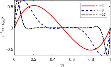
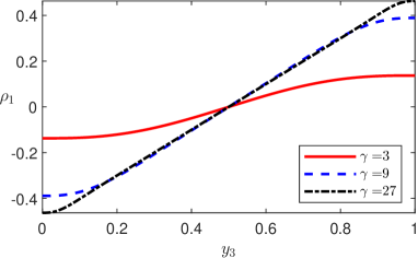
Figure 2: (a) Normalized leading order approximation of the longitudinal velocity $\frac{v_{1,1}\partial_{y_{1}}\bar{\rho}}{\gamma}$ for various parameter $\gamma$. (b) $\rho_{1}$ for different $\gamma$.

As $\partial_{y_{1}}\bar{\rho}\rightarrow 0$, we have

$$v_{1,1}= -\frac{\text{Re}\mathrm{Ri}y_{3}(y_{3}-1)(2y_{3}-1)\cos(\theta)}{12}$$ (19)

$$-\frac{\text{Pe}\text{Re}^{2}\mathrm{Ri}^{2}y\left(2(y_{3}(2y_{3}-7)+7)y_{3}^{4}-7y_{3}+3\right)\sin(2\theta)\partial_{y_{1}}\bar{\rho}}{40320}+\mathcal{O}\left(\left(\partial_{y_{1}}\bar{\rho}\right)^{2}\right),$$

and

$$\rho_{1}= \frac{\text{Pe}\text{Re}\mathrm{Ri}\left(1-2y_{3}^{3}(3y_{3}(2y_{3}-5)+10)\right)\cos(\theta)\partial_{y_{1}}\bar{\rho}}{1440}+\mathcal{O}\left(\left(\partial_{y_{1}}\bar{\rho}\right)^{2}\right).$$ (20)

Therefore $v_{1,1}\sim\mathcal{O}(1)$, but $\rho_{1}\sim\mathcal{O}(\partial_{y_{1}}\bar{\rho})$. The leading order approximation of the longitudinal velocity and the density field are given by $v_{1}\sim v_{1,1}\partial_{y_{1}}\bar{\rho}=\mathcal{O}(\partial_{y_{1}}\bar{\rho})$ and $\rho\sim\rho_{1}\left(\partial_{y_{1}}\bar{\rho}\right)^{2}=\mathcal{O}\left(\left(\partial_{y_{1}}\bar{\rho}\right)^{2}\right)$, which confirms the ansatz of the asymptotic expansion (11).

Substituting the expansion of the velocity field and density field to equation (12) and notice that $\bar{v}_{1,1}=0$, the leading order approximation reads

$$\partial_{t}\bar{\rho}+\mathrm{Pe}\partial_{y_{1}}\left((\overline{v_{1,1}\rho_{1}}\left(\partial_{y_{1}}\bar{\rho}\right)^{2}\right)=\partial_{y_{1}}^{2}\bar{\rho}.$$ (21)

Computing the average yields

$$\overline{v_{1,1}\rho_{1}}=\frac{-\cot^{2}(\theta)}{2\gamma\text{Pe}\partial_{y_{1}}\bar{\rho}}\left(\frac{\sin(\gamma)\sinh(\gamma)}{(\sin(\gamma)+\sinh(\gamma))^{2}}+\frac{5(\cos(\gamma)-\cosh(\gamma))}{2\gamma(\sin(\gamma)+\sinh(\gamma))}+1\right).$$ (22)

The effective equation 21 for the averaged density field becomes

$$\partial_{t}\bar{\rho}=\partial_{y_{1}}\left(\kappa_{\mathrm{eff}}\partial_{y_{1}}\bar{\rho}\right),$$ (23)

$$\kappa_{\mathrm{eff}}=1+\cot^{2}(\theta)\left(\frac{\sin(\gamma)\sinh(\gamma)}{(\sin(\gamma)+\sinh(\gamma))^{2}}+\frac{5(\cos(\gamma)-\cosh(\gamma))}{2\gamma(\sin(\gamma)+\sinh(\gamma))}+1\right).$$

This equation can be considered as an generalization of the diffusion equation with replacing the constant diffusion coefficient by a positive define function that depends on the derivative of the solution. This equation is belong to the family of equation that takes the form $\partial_{t}w=f(\partial_{x}w)\partial_{x}^{2}w$, which occurs in the nonlinear theory of flows in porous media and also governs the motion of a nonlinear viscoplastic medium (See page 342 in Polyanin & Zaitsev (2012)).

To complete the leading order approximation for the whole system, we next consider the approximation for the transverse velocity and pressure. Once the leading order approximation the longitudinal velocity is known, we can calculate the transverse velocity via the continuity equation. Substituting the expansion (11) into the continuity equation and collecting the terms that is comparable to $\partial_{y_{1}}^{2}\bar{\rho}$ yields

$$\partial_{y_{1}}\left(v_{1,1}\partial_{y_{1}}\bar{\rho}\right)+\partial_{y_{3}}v_{3,2}\partial_{y_{1}}^{2}\bar{\rho}=0.$$ (24)

Recall the fact that $\bar{v}_{1,1}=0$. Using no-slip boundary condition yields the expression of $v_{3,2}$:

$$v_{3,2}=-\frac{\int\limits_{0}^{y_{3}}\partial_{y_{1}}\left(v_{1,1}\partial_{y_{1}}\bar{\rho}\right)\mathrm{d}y_{3}}{\partial_{y_{1}}^{2}\bar{\rho}}$$ (25)

$$=\frac{\cot(\theta)\gamma}{2\text{Pe}(\sin(\gamma)+\sinh(\gamma))^{2}\partial_{y_{1}}\bar{\rho}}\left(\sin(\gamma(1-y))\sinh(\gamma y)(y\sin(\gamma)+(y-1)\sinh(\gamma))\right.$$

$$\hskip 113.81102pt\left.-\sin(\gamma y)\sinh(\gamma(1-y))\left((y-1)\sin(\gamma)+y\sinh(\gamma)\right)\right).$$

In the limit $\partial_{y_{1}}\bar{\rho}\rightarrow 0$, we have

$$v_{3,2}= \frac{1}{24}\text{Re}\text{Ri}(y_{3}-1)^{2}y_{3}^{2}\cos(\theta)$$ (26)

$$+\frac{\text{Pe}\text{Re}^{2}\text{Ri}^{2}y_{3}^{2}\left(y_{3}-1\right)^{2}\left(3y_{3}^{4}-6y_{3}^{3}-y_{3}^{2}+4y_{3}+9\right)\sin(2\theta)\partial_{y_{1}}\bar{\rho}}{120960}+\mathcal{O}\left(\left(\partial_{y_{1}}\bar{\rho}\right)^{2}\right).$$

Therefore, $v_{3}\sim v_{3,2}\partial_{y_{1}}^{2}\bar{\rho}=\mathcal{O}(\partial_{y_{1}}^{2}\bar{\rho})$, consistent with the assumption regarding the order of magnitude in the expansion given by (11).

$p_{1}$ in the expansion of pressure provided in equation (11) satisfies

$$-\partial_{y_{3}}p_{1}-\cos(\theta)\mathrm{Ri}\mathrm{Re}\rho_{1}=0.$$ (27)

The solution is

$$p_{1}=\cot(\theta)\text{cos}(\theta)\mathrm{Ri}\mathrm{Re}\left(\frac{1}{12}+\frac{1}{2}(y-1)y+\right.$$ (28)

$$\left.\frac{\sin(\gamma-\gamma y)\cosh(\gamma y)-\cos(\gamma-\gamma y)\sinh(\gamma y)-\cos(\gamma y)\sinh(\gamma-\gamma y)+\sin(\gamma y)\cosh(\gamma-\gamma y)}{2\gamma^{2}(\sin(\gamma)+\sinh(\gamma))}\right).$$

In the limit $\partial_{y_{1}}\bar{\rho}\rightarrow 0$, we have

$$p_{1}= \frac{-\cos^{2}\theta\text{Pe}\text{Re}^{2}\text{Ri}^{2}\left(28y_{3}^{6}-84y_{3}^{5}+70y_{3}^{4}-14y_{3}+3\right)\partial_{y_{1}}\bar{\rho}}{20160}+\mathcal{O}\left(\left(\partial_{y_{1}}\bar{\rho}\right)^{2}\right).$$ (29)

3.3 Numerical simulation

In this subsection, we perform simulations of the full governing equation (6) to demonstrate both the accuracy and validity of our asymptotic approximation and the effective equation (23).

The Boussinesq approximation is a well-established method for analyzing buoyancy-driven flow (Deen (1998)), as well as in earlier studies on steady diffusion-driven flow by Phillips (1970) and Wunsch (1970). While the theoretical results presented in the previous section do not rely on the Boussinesq approximation, we have chosen to utilize this approximation in our numerical simulations for the sake of simplicity. This approximation assumes that density variations primarily affect the buoyancy term and can be neglected in other terms. Its validity hinges on the condition that the relative change in density is small, i.e., $\Delta\rho\ll 1$. Fortunately, this condition holds true within the parameter regime of our interest. For instance, a study by Abaid et al. (2004) measured the density of a sodium chloride solution using the formula $\rho=0.9971+0.00065S+0.000322(25-T)$ g/cm³, where salinity $S$ is expressed in parts per thousand (ppt) and temperature $T$ is in ^∘C. Even for solutions with extremely high salinity, the density remains close to 1.19 g/cm${}^{3}($Hall (1924)). Therefore, adopting the Boussinesq approximation is a reasonable and justifiable choice.

To solve the Navier-Stokes equation (6), we employ the projection algorithm. During each iteration, we explicitly evaluate the advection term, while treating the viscosity term implicitly. This involves solving a Poisson equation while enforcing the no-slip boundary condition. Subsequently, we solve the pressure Poisson equation, wherein adjustments are made to the velocity field to ensure fulfillment of the incompressibility condition. A comprehensive outline of the numerical scheme can be found in Hecht et al. (2005). We employ a similar approach for the advection-diffusion equation. In each step, the advection term is explicitly computed, whereas the diffusion term is treated implicitly, necessitating the resolution of a Poisson equation with a no-flux boundary condition. The finite element method is used to discretize the system of equations, and we implement the algorithm using the software FreeFEM++ (Hecht (2012)).

The computational domain is defined as $\left\{(y_{1},y_{3})|y_{1}\in[-5,5],y_{3}\in[0,1]\right\}$. This domain is discretized using a triangular mesh with nearly uniform mesh sizes across the entire domain. In a typical simulation, the mesh consists of 17,594 vertices and 34,286 triangles. The simulation employs P1 elements, which correspond to linear functions defined over the triangles.

In the Boussinesq approximation, the solution remains unchanged when a constant is added to the density field. Consequently, we choose the initial condition for the averaged density field to be $\bar{\rho}_{I}(y_{1})=\frac{1}{2}\mathrm{erfc}(y_{1})$ for the sake of convenience. To expedite the system’s convergence to its asymptotic state, we initialize it with the leading-order approximations of the velocity, density, and pressure fields as outlined in equation (18). These initial conditions are depicted in the first row of Figure 3. Since density gradient is large around $y_{1}=0$, the flow is also localized in that regime. The third row of Figure 3 displays the density field and velocity field obtained by the simulation at $t=5$, with the time step size $0.004$ and specified parameters

$$\mathrm{Re}=1,\quad\mathrm{Ri}=400,\quad\mathrm{Pe}=40,\quad\mathrm{Sc}=1,\quad\theta=\frac{\pi}{4}.$$ (30)

As time increases, the density field becomes smoother and a large fluid circulation is formed in this whole domain.

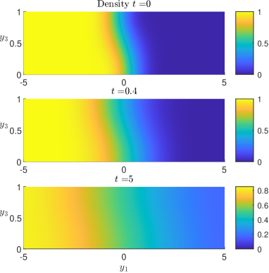
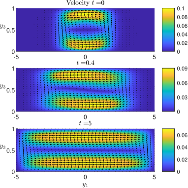
Figure 3: In the left panel, we display the density field at three time instances: $t=0$ (top), $t=0.4$ (middle) and $t=5$ (bottom). In the right panel, a pseudocolor plot illustrates the magnitude of the velocity field at the same time points: $t=0$ (top), $t=0.4$ (middle) and $t=5$ (bottom).

To proceed, we must simulate the effective equation (23) for comparison with the simulation of the governing equation (6). We employ the Fourier spectral method, as detailed in the work by Ding & McLaughlin (2022a), which incorporates a third-order Runge-Kutta scheme (Pareschi & Russo (2005)). Specifically, we utilize the explicit Runge-Kutta method for integrating the nonlinear terms, while the diffusion term is handled using the implicit Runge-Kutta method. To ensure a meaningful comparison between our simulations and those based on the complete governing equations, we specify our computational domain as $y_{1}\in[-5,5]$. Additionally, we enforce no-flux boundary conditions at the endpoints of this interval to guarantee the conservation of mass. The Fourier spectral method is particularly effective for periodic domains, but we encounter no-flux boundary conditions in the $y_{1}$-direction. To overcome this problem, we implement an even extension to establish periodic conditions on the extended domain $[-5,15]$, which ensures the no-flux boundary condition on the original domain $[-5,5]$. The original domain comprises $2^{10}+1$ grid points, while the extended domain encompasses $2^{11}$ grid points. The typical grid size is $0.0098$, and the typical time step size is $9.7561\times 10^{-5}$.

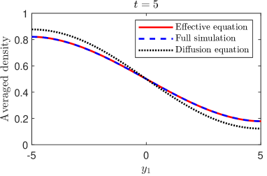
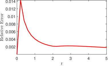
Figure 4: In the left panel, we present the solution of the effective equation (23) (represented by the red solid curve), the cross-sectional averaged density field derived from simulating the complete governing equation (illustrated by the blue dashed curve), and the solution to the diffusion equation (depicted by the black dotted curve) at the time instant $t=5$. Moving to the right panel, we showcase the temporal evolution of the relative difference between the solution of the effective equation and the cross-sectional averaged density field obtained through the full simulation. This relative difference is defined as the maximum deviation between the functions across the domain divided by the maximum value of the averaged density field obtained from the full simulation.

In Figure 4, the left panel offers a comprehensive comparison. Here, we solve the solution of effective equation (23) with the same parameters (30), and superimpose it with the cross-sectional averaged density field obtained through simulation of the complete governing equation (6) at the time instance $t=5$. The remarkable alignment between these curves serves to underscore the accuracy of the effective equation as an adept approximation for the full system. Additionally, we include the solution corresponding to the pure diffusion equation (representing the case in the absence of fluid flow) within the same visual representation. Notably, the contrast between the pure diffusion solution and the effective equation’s solution demonstrates a significant enhancement of fluid mixing through diffusion-driven flow.

Shifting our attention to the right panel of Figure 4, we delve into the temporal dynamics of the relative difference between the effective equation’s solution and the full system’s solution. At the inception ($t=0$), this disparity is nil, attributed to identical initial conditions. During the initial stages, the relative difference magnifies as the system has yet to transition into the regime well-captured by the effective equation. Nevertheless, even during this phase, the maximum relative difference remains at approximately 0.0143. As the system approaches an asymptotic state, which occurs after the diffusion time scale ($t=1$), the relative difference diminishes, stabilizing at around 0.002 until the simulation’s culmination. It’s worth noting that due to the assumption of the asymptotic analysis, the effective equation is valid for small density gradient $\partial_{y_{1}}\rho\ll 1$. In this numerical test case, we have $\max\limits_{y_{1},t}\partial_{y_{1}}\rho=\frac{1}{\sqrt{\pi}}\approx 0.6419$, indicating that the parameter regime for the effective equation to reach a good approximation is larger than previously thought.

To demonstrate the validity of the effective equation across a wide range of parameters, we conducted simulations using a different set of nondimensional parameters,

$$\mathrm{Re}=0.1,\quad\mathrm{Ri}=50000,\quad\mathrm{Pe}=100,\quad\mathrm{Sc}=1,\quad\theta=\frac{\pi}{4}.$$ (31)

The velocity field results are presented in the left panel of Figure 5. Comparing Figure 3 with Figure 5, we make two observations: First, as $\mathrm{Ri}$ increases, the velocity field exhibits more intricate structures during the initial stages. A distinctive ’S’ shape curve forms in the middle of the pseudocolor plot of the velocity field and stretches in subsequent time instants. Second, at $t=5$, panel (b) of Figure 3 illustrates that the velocity field is antisymmetric with respect to $y_{3}=\frac{1}{2}$. However, in panel (a) of Figure 5, at $t=5$, the velocity field is not antisymmetric with respect to $y_{3}=\frac{1}{2}$ near the corner of the domain.

In the figure at the top of panel (b) of Figure 5, we display the relative difference between the magnitude of the velocity field and its leading-order approximation. The error is relatively small within the interior of the domain but becomes significant near the corners. This discrepancy arises because the leading-order approximation of velocity is antisymmetric across the entire domain while the actual velocity field is not. To achieve a more precise approximation, it becomes necessary to incorporate boundary layer corrections near the corners into the density approximation.

One might assume that the substantial error in velocity approximation near the corners could significantly compromise the accuracy of other approximations. However, as shown in the figure at the bottom of panel (b) of Figure 5, the relative error in the approximation of the averaged density remains small. We believe this is due to two possible reasons: Firstly, the error in the velocity field approximation is localized near the corner of the domain, constituting a relatively small portion of the overall domain. Consequently, it has a limited impact on the entire dynamics process. Secondly, the error may cancel out when averaging along the transverse direction of the domain.

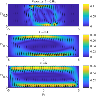
Figure 5: In the left panel, a pseudocolor plot illustrates the magnitude of the velocity field at three time instances: $t=0.04$ (top), $t=0.4$ (middle) and $t=5$ (bottom). In the right panel, the top figure shows the relative approximation error of the speed. The figure at the bottom showcase the temporal evolution of the relative error of the averaged density field.

4 Analysis of the effective equation

After confirming the accuracy of the effective equation (23) for the density field through numerical simulations, this section delves deeper into its properties.

The behavior of equation (23) is primarily governed by $\kappa_{\mathrm{eff}}$. Its asymptotic expansions for small and large values of $\gamma$ are provided below:

$$\kappa_{\mathrm{eff}}=1+\cot^{2}(\theta)\left(\left(1-\frac{5}{2\gamma}\right)+\frac{(2\gamma+5)\sin(\gamma)+5\cos(\gamma)}{\gamma e^{\gamma}}+\mathcal{O}\left(\gamma^{2}e^{-\gamma}\right)\right),\;\gamma\rightarrow\infty,$$ (32)

$$\kappa_{\mathrm{eff}}=1+\cot^{2}(\theta)\left(\frac{\gamma^{8}}{22680}-\frac{2879\gamma^{12}}{4086482400}+\mathcal{O}\left(\gamma^{16}\right)\right),\quad\gamma\rightarrow 0.$$

Figure 6 shows the graph of $\frac{\kappa_{\mathrm{eff}}-1}{\cot^{2}(\theta)}$ and its approximations as a function of $\gamma$. By examining both the graph and the asymptotic approximations, we can conclude that for $\gamma\geq 0$:

$$1\leq\kappa_{\mathrm{eff}}(\gamma)<1+\cot^{2}(\theta).$$ (33)

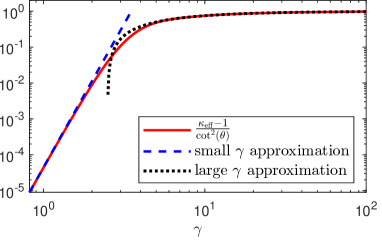
Figure 6: The red solid curve represents $\frac{\kappa_{\mathrm{eff}}-1}{\cot^{2}(\theta)}$ as a function of the nondimensional parameter $\gamma=\frac{1}{\sqrt{2}}\left(-\mathrm{Re}\mathrm{Pe}\mathrm{Ri}\sin\theta\partial_{y_{1}}\bar{\rho}\right)^{\frac{1}{4}}$. For small values of $\gamma$, the corresponding approximation is $\frac{\gamma^{8}}{22680}$, which is depicted by the blue dashed curve. Conversely, for large values of $\gamma$, the corresponding approximation is $1-\frac{5}{2\gamma}$, illustrated by the black dotted curve.

For large values of $\gamma$, equation (23) becomes a diffusion equation with an enhanced diffusion coefficient:

$$\partial_{t}\bar{\rho}=\left(1+\cot^{2}\theta\right)\partial_{y_{1}}^{2}\bar{\rho}.$$ (34)

This resembles the scenario of a passive scalar governed by an advection-diffusion equation with a prescribed velocity field. In the context of the channel domain and at diffusion time scales, the advection-diffusion equation can be effectively simplified to a diffusion equation with an enhanced effective diffusion coefficient (see Chatwin (1970); Smith (1982); Young & Jones (1991); Ding et al. (2021); Ding & McLaughlin (2022b) for related work).

However, it’s important to note that $\gamma$ is not a constant; it depends on the density gradient. Therefore, the diffusion equation (34) cannot provide a uniform approximation of the effective equation for all time instances. As time progresses, the stratified scalar becomes more homogeneous across the domain. As the density gradient decreases, $\gamma$ decreases, and the approximation given by (34) becomes less accurate.

To illustrate this, we conducted simulations with the parameters provided in equation (31) as an example. The left panel in figure 7 shows the maximum value of $\gamma$ across the domain as a function of time. As we expect, it is a decreasing function. The middle panel of figure 7 demonstrates that the solution to the diffusion equation (34) reasonably approximates the solution to the effective equation (23) initially. However, as time progresses and the density gradient decreases, $\max\limits_{y_{1}}\gamma$ also decreases. At $t=5$, the difference between the solution of equation (34) and that of equation (23) becomes more pronounced. This example also demonstrate that a single diffusion equation is not enough to accurately describes the dynamics of the averaged density field at all different time scale.

Equation (34) suggests that as the inclination angle approaches zero, the dispersion rate may increase, possibly reaching infinity. It’s crucial to emphasize that this conclusion holds true even when other parameters are kept constant. However, it’s worth noting that as the inclination angle decreases, maintaining the same value of $\gamma$ necessitates keeping the same density variation in the $y_{1}$ direction, which in turn requires a larger density variation in the $x_{3}$ direction. Achieving such a condition in practical applications can pose significant challenges.

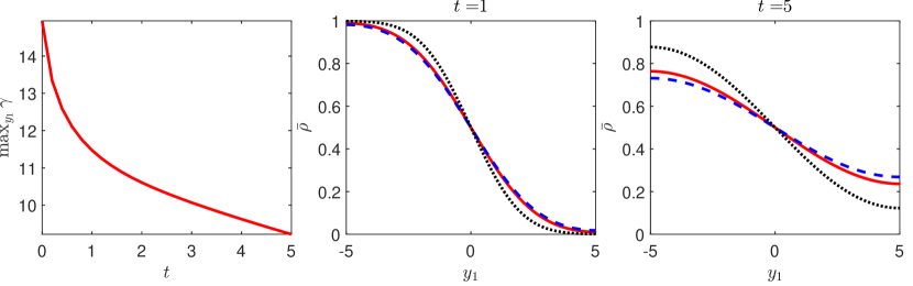
Figure 7: The left panel in figure 7 shows $\max\limits_{y_{1}}\gamma$ as a function of time. The middle panel presents the solution of the effective equation (23) (represented by the red solid curve), the solution of diffusion equation with diffusivity $1+\cot^{2}(\theta)$ (illustrated by the blue dashed curve), and the solution to the diffusion equation with diffusivity 1 (depicted by the black dotted curve) at the time instant $t=1$. The right panel shows the corresponding curves at the time instant $t=5$.

Next we consider the case with small $\gamma$. In this limit, the effective equation for the density field (23) reduces to

$$\partial_{t}\bar{\rho}=\partial_{y_{1}}\left(\left(1+\left(\frac{\mathrm{Ri}\text{Pe}\text{Re}\cos(\theta)}{72\sqrt{70}}\partial_{y_{1}}\bar{\rho}\right)^{2}\right)\partial_{y_{1}}\bar{\rho}\right).$$ (35)

The closed form expression of the solution of this equation is not available. However, we can obtain the solution in some limits for unbounded domain. When the nonlinear term is much larger than the diffusion term, namely, $\frac{\mathrm{Ri}\text{Pe}\text{Re}\cos(\theta)}{72\sqrt{70}}\partial_{y_{1}}\bar{\rho}\gg 1$, equation (35) can be approximated by

$$\partial_{t}\bar{\rho}=\partial_{y_{1}}\left(\alpha^{2}\left(\partial_{y_{1}}\bar{\rho}\right)^{3}\right),\quad\alpha=\frac{\mathrm{Ri}\text{Pe}\text{Re}\cos(\theta)}{72\sqrt{70}}.$$ (36)

We can look for the self similarity solution, $\rho(y_{1},t)=f\left(\xi\right)$, where $\xi=ty_{1}^{-\frac{1}{4}}$. Equation (36) becomes

$$f^{\prime}(\xi)\left(12\alpha^{2}f^{\prime}(\xi)f^{\prime\prime}(\xi)+\xi\right)=0.$$ (37)

The solution is

$$f(\xi)=\begin{cases}c_{2}+\pi c_{1}\alpha\sqrt{3}&\xi\geq 2\alpha\sqrt{6c_{1}},\\ c_{2}-\frac{\frac{1}{2}\xi\sqrt{24\alpha^{2}c_{1}-\xi^{2}}+12\alpha^{2}c_{1}\tan^{-1}\left(\frac{\xi}{\sqrt{24\alpha^{2}c_{1}-\xi^{2}}}\right)}{2\sqrt{3}\sqrt{\alpha}}&-2\alpha\sqrt{6c_{1}}\leq\xi\leq 2\alpha\sqrt{6c_{1}},\\ c_{2}-\pi c_{1}\alpha\sqrt{3}&\xi\leq-2\alpha\sqrt{6c_{1}},\end{cases}$$ (38)

where $c_{1}$, $c_{2}$ are the constants that can be defined by the boundary condition at infinity. For the case $\bar{\rho}(\infty)=0$ and $\bar{\rho}(-\infty)=1$, we have $c_{1}=\frac{1}{2\sqrt{3}\pi\alpha}$, $c_{2}=\frac{1}{2}$. Notice that the similarity variable for the pure diffusion equation is $\xi=\frac{y_{1}}{\sqrt{t}}$. Therefore, $t\rightarrow\infty$, the neglected diffusion term in the above calculation becomes dominant eventually.

Last, we can represent $\gamma$ in terms of the physical parameters as follows: $\gamma=\frac{1}{\sqrt{2}}\left(\frac{gL^{3}\rho_{0}}{\kappa\mu}\sin\theta\partial_{y_{1}}\bar{\rho}\right)^{\frac{1}{4}}$. Therefore, smaller diffusivity, lower viscosity, greater gravitational constant, larger gap thickness, and higher density result in a larger value of $\gamma$. We can calculate $\gamma$ using the practical parameters provided in equation (8). If we set $\theta=\frac{\pi}{4}$ and estimate the density gradient as $\partial_{y_{1}}\bar{\rho}=\frac{\Gamma L\sin\theta}{\rho_{0}}$, we obtain $\gamma\approx 4.88974$. In this case, we cannot employ the approximate equations (34) and (35). Instead, we must use the complete effective equation (23) to solve for the density field.

4.1 Long time behavior of the solution

As demonstrated in our previous examples, diffusion-driven flow enhances the mixing of a stratified scalar at some time scales. One might expect the difference between the density profile with and without the fluid to increase as time progresses or at least persist at long times. However, intriguingly, this difference actually vanishes over extended periods.

To understand this, it’s essential to recall an interesting observation that emerges when considering various solutions to the diffusion equation. Under some conditions, these solutions converge to a self-similarity solution asymptotically at long times, as discussed in Newman (1984). To illustrate this point, consider two solutions: $f_{1}=\frac{1}{2}\text{erfc}\left(\frac{x}{2\sqrt{t}}\right)$ and $f_{2}=\frac{1}{2}\text{erfc}\left(\frac{x}{2\sqrt{\sigma^{2}+t}}\right)$, both satisfying the diffusion equation $\partial_{t}f=\partial_{x}^{2}f$. Although they begin with different initial conditions, the relative difference between them diminishes as $t\rightarrow\infty$:

$$\frac{f_{1}-f_{2}}{f_{1}}=\frac{\sigma^{2}xt^{-\frac{3}{2}}}{2\sqrt{\pi}}+\mathcal{O}\left(t^{-2}\right).$$ (39)

The timescale for this convergence depends on the difference in the initial conditions and can be multiple times the diffusion time scale.

This observation implies that even if diffusion-driven flow initially amplifies the dispersion of the stratified agent, when the density gradient is sufficiently weak, the governing equation for the density field approximates a diffusion equation with a diffusivity of 1. While some disparity remains between the solution of the effective equation and the solution of the pure diffusion equation, this difference diminishes over longer time scales.

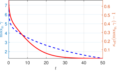
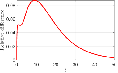
Figure 8: (a)The blue dashed curve represents $\max_{y_{1}}\gamma$ and is associated with the left $y$ axis. The read solid curve represents $\kappa_{\mathrm{eff}}(\max_{y_{1}}\gamma)-1$ and is associated with the right $y$ axis. (b) The relative difference between the density profile with and without the fluid as a function of time.

To confirm this conclusion, we solve the effective equation (23) with the parameters provided in equation (30). In Panel (a) of Figure 8, we plot $\max_{y_{1}}\gamma$ and $\kappa_{\mathrm{eff}}(\max_{y_{1}}\gamma)-1$ as functions of time, providing an estimation of the enhancement of dispersion induced by diffusion-driven flow. We observe that the enhancement decrees below 0.1 after $t>20$, which implies the effective equation is close to the pure diffusion equation after that time. In Panel (b) of Figure 8, we display the relative difference between the density profiles with and without flow. This difference initially increases, reaching its maximum around $t=10$, but subsequently decreases to 0.003 at $t=50$.

This result demonstrate that in a confined domain with no-flux boundary condition, the density profile in a system with the diffusion driven flow asymptotically converges to the one without the flow at extremely large time scale.

5 Comparison to the thin film approximation

As previously mentioned, we can employ the classical asymptotic expansion to analyze the governing equation (6). In this section, we will utilize the thin film approximation and subsequently compare the results with those obtained previously.

In the thin film approximation, we select distinct length scales in different directions for the purpose of nondimensionalization.

$$L_{i}y_{i}^{\prime}=y_{i},\quad V_{i}v_{i}^{\prime}=v_{i},\quad\frac{\rho_{0}L_{1}\nu U}{L_{3}^{2}}p^{\prime}=p,\quad\frac{L_{1}^{2}}{\kappa}t^{\prime}=t,\quad\rho_{0}\rho^{\prime}=\rho$$ (40)

$$\epsilon=\frac{V_{3}}{V_{1}}=\frac{L_{3}}{L_{1}},\quad\mathrm{Re}=\frac{V_{1}L_{3}}{\nu},\quad\mathrm{Pe}=\frac{V_{1}L_{3}}{\kappa},\quad\mathrm{Sc}=\frac{\mu}{\rho_{0}\kappa},\quad\mathrm{Ri}=\frac{L_{3}g}{V_{1}^{2}}.$$

The nondimensionalized governing equation becomes

$$\rho^{\prime}\left(\frac{\epsilon^{2}}{\mathrm{Sc}}\partial_{t^{\prime}}v_{1}^{\prime}+\epsilon\mathrm{Re}\left(v_{1}^{\prime}\partial_{y_{1}^{\prime}}v_{1}^{\prime}+v_{3}^{\prime}\partial_{y_{3}^{\prime}}v_{1}^{\prime}\right)\right)=\left(\epsilon^{2}\partial_{y_{1}^{\prime}}^{2}v_{1}^{\prime}+\partial_{y_{3}^{\prime}}^{2}v_{1}^{\prime}\right)-\partial_{y_{1}^{\prime}}p^{\prime}-\mathrm{Re}\mathrm{Ri}\rho^{\prime}\sin\theta,$$ (41)

$$\rho^{\prime}\left(\frac{\epsilon^{3}}{\mathrm{Sc}}\partial_{t^{\prime}}v_{3}^{\prime}+\epsilon^{2}\mathrm{Re}\left(v_{1}^{\prime}\partial_{y_{1}^{\prime}}v_{3}^{\prime}+v_{3}^{\prime}\partial_{y_{3}^{\prime}}v_{3}^{\prime}\right)\right)=\left(\epsilon^{3}\partial_{y_{1}^{\prime}}^{2}v_{3}^{\prime}+\epsilon\partial_{y_{3}^{\prime}}^{2}v_{3}^{\prime}\right)-\frac{1}{\epsilon}\partial_{y_{3}^{\prime}}p^{\prime}-\mathrm{Re}\mathrm{Ri}\rho^{\prime}\cos\theta,$$

$$\epsilon^{2}\partial_{t^{\prime}}\rho^{\prime}+\epsilon\mathrm{Pe}v_{1}^{\prime}\partial_{y_{1}^{\prime}}\rho^{\prime}+\epsilon\mathrm{Pe}v_{3}^{\prime}\partial_{y_{3}^{\prime}}\rho^{\prime}=\epsilon^{2}\partial_{y_{1}^{\prime}}^{2}\rho^{\prime}+\partial_{y_{3}^{\prime}}^{2}\rho^{\prime}.$$

Dropping primes and rearranging the equation results

$$\rho\left(\frac{\epsilon^{2}}{\mathrm{Sc}}\partial_{t}v_{1}+\epsilon\mathrm{Re}\left(v_{1}\partial_{y_{1}}v_{1}+v_{3}\partial_{y_{3}}v_{1}\right)\right)=\left(\epsilon^{2}\partial_{y_{1}}^{2}v_{1}+\partial_{y_{3}}^{2}v_{1}\right)-\partial_{y_{1}}p-\mathrm{Re}\mathrm{Ri}\rho\sin\theta,$$ (42)

$$\rho\left(\frac{\epsilon^{4}}{\mathrm{Sc}}\partial_{t}v_{3}+\epsilon^{3}\mathrm{Re}\left(v_{1}\partial_{y_{1}}v_{3}+v_{3}\partial_{y_{3}}v_{3}\right)\right)=\epsilon^{2}\left(\epsilon^{2}\partial_{y_{1}}^{2}v_{3}+\partial_{y_{3}}^{2}v_{3}\right)-\partial_{y_{3}}p-\epsilon\mathrm{Re}\mathrm{Ri}\rho\cos\theta,$$

$$\epsilon^{2}\partial_{t}\rho+\epsilon\mathrm{Pe}\left(v_{1}\partial_{y_{1}}\rho+v_{3}\partial_{y_{3}}\rho\right)=\epsilon^{2}\partial_{y_{1}}^{2}\rho+\partial_{y_{3}}^{2}\rho,$$

$$\partial_{y_{1}}v_{1}+\partial_{y_{3}}v_{3}=0.$$

We consider the formal power series expansions for the velocity, density and pressure,

$$v_{i}=\sum\limits_{k=0}^{\infty}v_{i,k}\epsilon^{k},\quad\rho=\sum\limits_{k=0}^{\infty}\rho_{k}\epsilon^{k},\quad p=\sum\limits_{k=0}^{\infty}p_{k}\epsilon^{k}.$$ (43)

We have $\left.v_{i,k}\right|_{\mathbf{y}\in\partial\Omega}=0$ from the no-lip boundary condition of the velocity field, and $\left.\partial_{\mathbf{n}}\rho_{k}\right|_{\mathbf{y}\in\partial\Omega}=0$ from the no-flux boundary condition of the density field.

Substituting the expansion into the governing equation and collecting $\mathcal{O}(1)$ terms yields the following equation

$$0=\partial_{y_{3}}^{2}v_{1,0}-\partial_{y_{1}}p_{0}-\mathrm{Re}\mathrm{Ri}\rho_{0}\sin\theta,\;0=\partial_{y_{3}}p_{0},\;0=\partial_{y_{3}}^{2}\rho_{0},\;\partial_{y_{1}}v_{1,0}+\partial_{y_{3}}v_{3,0}=0.$$ (44)

There are two possible group of solutions:

$$v_{1,0}=v_{3,0}=0,\quad p_{0}=\mathrm{Re}\mathrm{Ri}\sin\theta\int\limits_{0}^{y_{1}}\rho_{0}\mathrm{d}y_{1},$$ (45)

and

$$v_{1,0}=Cy_{3}(y_{3}-1),\;v_{3,0}=0,\quad p_{0}=-2Cy_{1}+\mathrm{Re}\mathrm{Ri}\sin\theta\int\limits_{0}^{y_{1}}\rho_{0}\mathrm{d}y_{1},$$ (46)

where $C$ is a constant number and $\rho_{0}$ is independent of $y_{3}$. The second solution describes a flow generated by a constant pressure gradient, which does not represent the correct physical problem. Therefore, we regard the first solution as the correct leading-order approximation.

Collecting the terms that is comparable to $\mathcal{O}(\epsilon)$ yields the following equation

$$\mathrm{Re}\rho_{0}\left(v_{1,0}\partial_{y_{1}}v_{1,0}+v_{3,0}\partial_{y_{3}}v_{1,0}\right)=\partial_{y_{3}}^{2}v_{1,1}-\partial_{y_{1}}p_{1}-\mathrm{Re}\mathrm{Ri}\rho_{1}\sin\theta,$$ (47)

$$0=-\partial_{y_{3}}p_{1}-\mathrm{Re}\mathrm{Ri}\rho_{0}\cos\theta,\quad\mathrm{Pe}\left(v_{1,0}\partial_{y_{1}}\rho_{0}+v_{3,0}\partial_{y_{3}}\rho_{0}\right)=\partial_{y_{3}}^{2}\rho_{1},$$

$$\partial_{y_{1}}v_{1,1}+\partial_{y_{3}}v_{3,1}=0.$$

Using the conclusions (46) reduces the above equation to

$$0=\partial_{y_{3}}^{2}v_{1,1}-\partial_{y_{1}}p_{1}-\mathrm{Re}\mathrm{Ri}\rho_{1}\sin\theta,\quad 0=-\partial_{y_{3}}p_{1}-\mathrm{Re}\mathrm{Ri}\rho_{0}\cos\theta,$$ (48)

$$0=\partial_{y_{3}}^{2}\rho_{1},\quad\partial_{y_{1}}v_{1,1}+\partial_{y_{3}}v_{3,1}=0.$$

Similar as the equation for $\mathcal{O}(1)$ terms, the solution is not unique. To eliminate the solution representing the pressure driven flow, we impose the condition $\bar{p}_{1}=0$. From the second equation, we have

$$p_{1}=-\left(y_{3}-\frac{1}{2}\right)\mathrm{Re}\mathrm{Ri}\rho_{0}\cos\theta.$$ (49)

Averaging the first equation yields $\bar{v}_{1,1}=0$. Differentiating the first equation in equation (48) with respect to $y_{3}$ twice give us

$$0=\partial_{y_{3}}^{4}v_{1,1},\quad\left.v_{1,1}\right|_{y=0,1}=0,\quad\left.\partial_{y_{3}}^{3}v_{1,1}\right|_{y=0,1}=-\mathrm{Re}\mathrm{Ri}\cos\theta\partial_{y_{1}}\rho_{0}.$$ (50)

The solution is

$$v_{1,1}=-\mathrm{Re}\mathrm{Ri}\cos\theta\partial_{y_{1}}\rho_{0}\frac{y_{3}(y_{3}-1)(2y_{3}-1)}{12},$$ (51)

which is consistent with the first term in equation (19). From the third equation, we conclude that $\rho_{1}$ is independent of $y_{3}$. Moreover, after substituting the expression of $v_{1,1}$ back to the first equation in equation (48), we obtain $\rho_{1}=0$. The continuity equation gives us the expression of $v_{3,1}$:

$$v_{3,1}=-\int\limits_{0}^{y_{3}}\partial_{y_{1}}v_{1,1}\mathrm{d}y_{3}=\mathrm{Re}\mathrm{Ri}\cos\theta\partial_{y_{1}}^{2}\rho_{0}\frac{y_{3}^{2}(y_{3}-1)^{2}}{24},$$ (52)

which is consistent with the first term in equation (26). It’s important to note that the definition of $v_{3,1}$ in section 3 differs from the one presented here.

Collecting the terms that is comparable to $\mathcal{O}(\epsilon^{2})$ yields the following equation

$$\frac{\rho_{0}}{\mathrm{Sc}}\partial_{t}v_{1,0}+\mathrm{Re}\rho_{0}\left(v_{1,0}\partial_{y_{1}}v_{1,1}+v_{1,1}\partial_{y_{1}}v_{1,0}+v_{3,0}\partial_{y_{3}}v_{1,1}+v_{3,1}\partial_{y_{3}}v_{1,0}\right)$$ (53)

$$+\mathrm{Re}\rho_{1}\left(v_{1,0}\partial_{y_{1}}v_{1,0}+v_{3,0}\partial_{y_{3}}v_{1,0}\right)=\left(\partial_{y_{1}}^{2}v_{1,0}+\partial_{y_{3}}^{2}v_{1,2}\right)-\partial_{y_{1}}p_{2}-\mathrm{Re}\mathrm{Ri}\rho_{2}\sin\theta,$$

$$0=\partial_{y_{3}}^{2}v_{3,0}-\partial_{y_{3}}p_{2}-\mathrm{Re}\mathrm{Ri}\rho_{1}\cos\theta,$$

$$\partial_{t}\rho_{0}+\mathrm{Pe}\left(v_{1,0}\partial_{y_{1}}\rho_{1}+v_{1,1}\partial_{y_{1}}\rho_{0}+v_{3,0}\partial_{y_{3}}\rho_{1}+v_{3,1}\partial_{y_{3}}\rho_{0}\right)=\partial_{y_{1}}^{2}\rho_{0}+\partial_{y_{3}}^{2}\rho_{2},$$

$$\partial_{y_{1}}v_{1,2}+\partial_{y_{3}}v_{3,2}=0.$$

Using the current conclusions for $\mathcal{O}(\epsilon)$ terms, the above equation reduces to

$$0=\partial_{y_{3}}^{2}v_{1,2}-\partial_{y_{1}}p_{2}-\mathrm{Re}\mathrm{Ri}\rho_{2}\sin\theta,\quad 0=-\partial_{y_{3}}p_{2}-\mathrm{Re}\mathrm{Ri}\rho_{1}\cos\theta,$$ (54)

$$\partial_{t}\rho_{0}+\mathrm{Pe}v_{1,1}\partial_{y_{1}}\rho_{0}=\partial_{y_{1}}^{2}\rho_{0}+\partial_{y_{3}}^{2}\rho_{2}.$$

Notice that $\int\limits_{0}^{1}v_{1,1}\mathrm{d}y_{3}=0$ and $\rho_{0}$ is independent of $y_{3}$. Integrating on both side of the last equation in equation (54) with respect to $y_{3}$ and using the no-flux boundary conditions yields the evolution equation for $\rho_{0}$: $\partial_{t}\rho_{0}=\partial_{y_{1}}^{2}\rho_{0}$.

Now the last equation in equation (54) becomes $\mathrm{Pe}v_{1,1}\partial_{y_{1}}\rho_{0}=\partial_{y_{3}}^{2}\rho_{2}$ and implies

$$\rho_{2}=\frac{\mathrm{Pe}\text{Re}\text{Ri}\left(1-2y_{3}^{3}(10+3y_{3}(2y_{3}-5))\right)\cos(\theta)\left(\partial_{y_{1}}\rho_{0}\right)^{2}}{1440}.$$ (55)

which is consistent with the second term in equation (20). It’s important to note that the definition of $\rho_{1}$ in section 3 differs from the one presented here.

The density field approximation is expressed as $\rho=\rho_{0}+\epsilon^{2}\rho_{2}+\mathcal{O}(\epsilon^{3})$, which serves as the solution to a pure diffusion equation augmented by a higher order correction term. The fact that $\bar{\rho}_{2}=0$ implies that as $\epsilon$ tends to zero, the diffusion-driven flow only distorts the isopycnal of the density without amplifying the dispersion of the stratifying scalar in the longitudinal direction of the channel.

Last, since $\rho_{1}=0$, we have $p_{2}=0$ and the first equation in equation (54) gives

$$v_{1,2}=\frac{\text{Pe}\text{Re}^{2}\text{Ri}^{2}y_{3}\left(-2(y_{3}(2y_{3}-7)+7)y_{3}^{4}+7y_{3}-3\right)\sin(2\theta\left(\partial_{y_{1}}\rho_{0}\right)^{2}}{40320},$$ (56)

which is consistent with the second term in equation (19).

So far, we have observed that the results obtained from the thin film approximation are consistent with the results obtained in Section 3 when the density gradient vanishes, i.e., $\partial_{y_{1}}\bar{\rho}\rightarrow 0$, or equivalently when $\gamma\rightarrow 0$. Therefore, the thin film approximation presented here may not accurately model systems where the diffusion-driven flow significantly enhances dispersion, as is the case with the parameters provided in Equation (31), where the corresponding $\gamma=9\sim 15$ and the flow make visible enhancement of the scalar dispersion as shown in figure 7. For those parameter combinations, an asymptotic analysis using a different scaling relation for physical parameters become necessary.

6 Conclusion and discussion

This paper explores the diffusion-driven flow in a tilted parallel-plate channel domain with a nonlinear density stratification. By employing a novel asymptotic expansion provided in equation (11), we derive leading-order approximations for the velocity field (18) and (26), density field (18), and pressure field (28). Furthermore, we formulate an effective equation (23) to describe the cross-sectional averaged density field, and its accuracy is confirmed through numerical simulations of the governing equation (10).

The effective equation reveals that the dynamics of the density field depend on the dimensionless parameter $\gamma$, defined as $\gamma=\frac{1}{\sqrt{2}}\left(-\mathrm{Re}\mathrm{Pe}\mathrm{Ri}\sin\theta\partial_{y_{1}}\bar{\rho}\right)^{\frac{1}{4}}=\frac{1}{\sqrt{2}}\left(\frac{gL^{3}\rho_{0}}{\kappa\mu}\sin\theta\partial_{y_{1}}\bar{\rho}\right)^{\frac{1}{4}}$. When $\gamma$ is large, the system behaves akin to a diffusion equation with an enhanced diffusion coefficient of $1+\cot^{2}\theta$. This result reveals an upper bound for the mixing capability of the diffusion-driven flow. Conversely, in the small $\gamma$ limit, the behavior of the density field approximates a pure diffusion process, with the diffusion-driven flow failing to amplify the dispersion of the stratified agent significantly. Additionally, we demonstrate that in a confined domain with no-flux boundary conditions, the density profile in a system featuring diffusion-driven flow asymptotically converges to the one without flow over long times, although this convergence occurs on a timescale much larger than the diffusion time scale.

Moreover, we establish that the thin film approximation aligns with the results obtained using the novel expansion when the diffusion-driven flow is weak. In such scenarios, the density field can be modeled by a diffusion equation featuring molecular diffusivity, and the diffusion-driven flow primarily distorts the isopycnal without significantly increasing longitudinal dispersion. Consequently, the thin film approximation falls short in describing systems with relatively large density gradients, where diffusion-driven flow markedly enhances dispersion. Importantly, we both numerically and theoretically demonstrate that the proposed expansion effectively addresses these situations.

Future research directions encompass several avenues. Firstly, many channel domains feature rough wall boundaries, such as rock fissures. We aim to develop a reduced model that incorporates the characteristics of these rough boundaries. The multiscale method employed for analyzing the laminar flow problem could tackle this challenge (Achdou et al. (1998); Carney & Engquist (2022)). Secondly, while this work primarily focuses on analyzing parallel plate domains, it’s worth noting that the method proposed herein is applicable to channels with arbitrary cross-sections. Concentrating on the parallel plates domain stems from the availability of an exact solution for the auxiliary problem. Investigating this fundamental geometry can augment our understanding of domains with more complex shapes, such as tilted cylindrical cavities embedded in rocks Sánchez et al. (2005), or tilted square container (Grayer et al. (2020); Page (2011a, b); French (2017)).

7 Declaration of Interests

The authors report no conflict of interest.

References

- Abaid et al. (2004) Abaid, Nicole, Adalsteinsson, David, Agyapong, Akua & McLaughlin, Richard M 2004 An internal splash: Levitation of falling spheres in stratified fluids. Physics of Fluids 16 (5), 1567–1580.
- Achdou et al. (1998) Achdou, Yves, Pironneau, Olivier & Valentin, Frederic 1998 Effective boundary conditions for laminar flows over periodic rough boundaries. Journal of Computational Physics 147 (1), 187–218.
- Allshouse (2010) Allshouse, Michael R 2010 Novel applications of diffusion-driven flow. PhD thesis, Massachusetts Institute of Technology.
- Allshouse et al. (2010) Allshouse, Michael R, Barad, Michael F & Peacock, Thomas 2010 Propulsion generated by diffusion-driven flow. Nature Physics 6 (7), 516–519.
- Aref et al. (2017) Aref, Hassan, Blake, John R, Budišić, Marko, Cardoso, Silvana SS, Cartwright, Julyan HE, Clercx, Herman JH, El Omari, Kamal, Feudel, Ulrike, Golestanian, Ramin, Gouillart, Emmanuelle & others 2017 Frontiers of chaotic advection. Reviews of Modern Physics 89 (2), 025007.
- Aris (1956) Aris, Rutherford 1956 On the dispersion of a solute in a fluid flowing through a tube. Proceedings of the Royal Society of London. Series A. Mathematical and Physical Sciences 235 (1200), 67–77.
- Aulbach & Wanner (1996) Aulbach, Bernd & Wanner, Thomas 1996 Integral manifolds for Carathéodory type differential equations in Banach spaces. Six lectures on dynamical systems 2.
- Aulbach & Wanner (1999) Aulbach, Bernd & Wanner, Thomas 1999 Invariant foliations for Carathéodory type differential equations in banach spaces. Advances of Stability Theory at the End of XX Century’, Gordon & Breach Publishers. http://citeseerx. ist. psu. edu/viewdoc/download .
- Balakotaiah et al. (1995) Balakotaiah, Vemuri, Chang, Hsueh-Chia & Smith, FT 1995 Dispersion of chemical solutes in chromatographs and reactors. Philosophical Transactions of the Royal Society of London. Series A: Physical and Engineering Sciences 351 (1695), 39–75.
- Braunsfurth et al. (1997) Braunsfurth, MG, Skeldon, AC, Juel, A, Mullin, T & Riley, DS 1997 Free convection in liquid gallium. Journal of Fluid Mechanics 342, 295–314.
- Camassa et al. (2022) Camassa, Roberto, Ding, Lingyun, McLaughlin, Richard M, Overman, Robert, Parker, Richard & Vaidya, Ashwin 2022 Critical density triplets for the arrestment of a sphere falling in a sharply stratified fluid. Recent Advances in Mechanics and Fluid-Structure Interaction with Applications: The Bong Jae Chung Memorial Volume p. 69.
- Camassa et al. (2019) Camassa, Roberto, Harris, Daniel M, Hunt, Robert, Kilic, Zeliha & McLaughlin, Richard M 2019 A first-principle mechanism for particulate aggregation and self-assembly in stratified fluids. Nature communications 10 (1), 1–8.
- Carney & Engquist (2022) Carney, Sean P & Engquist, Björn 2022 Heterogeneous multiscale methods for rough-wall laminar viscous flow. Communications in Mathematical Sciences 20 (8), 2069–2106.
- Carr (2012) Carr, Jack 2012 Applications of centre manifold theory, , vol. 35. Springer Science & Business Media.
- Cenedese & Adduce (2008) Cenedese, Claudia & Adduce, Claudia 2008 Mixing in a density-driven current flowing down a slope in a rotating fluid. Journal of Fluid Mechanics 604, 369–388.
- Chashechkin (2018) Chashechkin, Yuli D 2018 Waves, vortices and ligaments in fluid flows of different scales. Physics & Astronomy International Journal 2 (2), 105–108.
- Chashechkin & Mitkin (2004) Chashechkin, Yu D & Mitkin, Vladimir V 2004 A visual study on flow pattern around the strip moving uniformly in a continuously stratified fluid. Journal of Visualization 7 (2), 127–134.
- Chatwin (1970) Chatwin, PC 1970 The approach to normality of the concentration distribution of a solute in a solvent flowing along a straight pipe. Journal of Fluid Mechanics 43 (2), 321–352.
- Deen (1998) Deen, William Murray 1998 Analysis of transport phenomena, , vol. 2. Oxford university press New York.
- Dell & Pratt (2015) Dell, RW & Pratt, LJ 2015 Diffusive boundary layers over varying topography. Journal of Fluid Mechanics 769, 635–653.
- Dimitrieva (2019) Dimitrieva, NF 2019 Stratified flow structure near the horizontal wedge. Fluid Dynamics 54, 940–947.
- Ding (2022) Ding, Lingyun 2022 Scalar transport and mixing. PhD thesis, The University of North Carolina at Chapel Hill.
- Ding (2023) Ding, Lingyun 2023 Shear dispersion of multispecies electrolyte solutions in the channel domain. Journal of Fluid Mechanics 970, A27.
- Ding et al. (2021) Ding, Lingyun, Hunt, Robert, McLaughlin, Richard M & Woodie, Hunter 2021 Enhanced diffusivity and skewness of a diffusing tracer in the presence of an oscillating wall. Research in the Mathematical Sciences 8 (3), 1–29.
- Ding & McLaughlin (2022a) Ding, Lingyun & McLaughlin, Richard M 2022a Determinism and invariant measures for diffusing passive scalars advected by unsteady random shear flows. Physical Review Fluids 7 (7), 074502.
- Ding & McLaughlin (2022b) Ding, Lingyun & McLaughlin, Richard M 2022b Ergodicity and invariant measures for a diffusing passive scalar advected by a random channel shear flow and the connection between the Kraichnan-Majda model and Taylor-Aris dispersion. Physica D: Nonlinear Phenomena 432, 133118.
- Ding & McLaughlin (2023) Ding, Lingyun & McLaughlin, Richard M. 2023 Dispersion induced by unsteady diffusion-driven flow in a parallel-plate channel. Phys. Rev. Fluids 8, 084501.
- Drake et al. (2020) Drake, Henri F, Ferrari, Raffaele & Callies, Jörn 2020 Abyssal circulation driven by near-boundary mixing: Water mass transformations and interior stratification. Journal of Physical Oceanography 50 (8), 2203–2226.
- French (2017) French, Alison 2017 Diffusion-driven flow in three dimensions. PhD thesis, Monash University.
- Gill (1967) Gill, WN 1967 A note on the solution of transient dispersion problems. Proceedings of the Royal Society of London. Series A. Mathematical and Physical Sciences 298 (1454), 335–339.
- Grayer et al. (2020) Grayer, Hezekiah, Yalim, Jason, Welfert, Bruno D & Lopez, Juan M 2020 Dynamics in a stably stratified tilted square cavity. Journal of Fluid Mechanics 883.
- Hall (1924) Hall, Ralph E 1924 The densities and specific volumes of sodium chloride solutions at 25°. Journal of the Washington Academy of Sciences 14 (8), 167–173.
- Hecht (2012) Hecht, Frédéric 2012 New development in freefem++. Journal of numerical mathematics 20 (3-4), 251–266.
- Hecht et al. (2005) Hecht, Frédéric, Pironneau, Olivier, Le Hyaric, A & Ohtsuka, K 2005 Freefem++ manual. Laboratoire Jacques Louis Lions .
- Heitz et al. (2005) Heitz, Renaud, Peacock, Thomas & Stocker, Roman 2005 Optimizing diffusion-driven flow in a fissure. Physics of Fluids 17 (12), 128104.
- Holmes et al. (2019) Holmes, Ryan M, de Lavergne, Casimir & McDougall, Trevor J 2019 Tracer transport within abyssal mixing layers. Journal of Physical Oceanography 49 (10), 2669–2695.
- Kistovich & Chashechkin (1993) Kistovich, AV & Chashechkin, Yu D 1993 The structure of transient boundary flow along an inclined plane in a continuously stratified medium. Journal of Applied Mathematics and Mechanics 57 (4), 633–639.
- Kondic (2003) Kondic, Lou 2003 Instabilities in gravity driven flow of thin fluid films. Siam review 45 (1), 95–115.
- Levitsky et al. (2019) Levitsky, VV, Dimitrieva, NF & Chashechkin, Yu D 2019 Visualization of the self-motion of a free wedge of neutral buoyancy in a tank filled with a continuously stratified fluid and calculation of perturbations of the fields of physical quantities putting the body in motion. Fluid Dynamics 54, 948–957.
- Lin et al. (2011) Lin, Zhi, Thiffeault, Jean-Luc & Doering, Charles R 2011 Optimal stirring strategies for passive scalar mixing. Journal of Fluid Mechanics 675, 465–476.
- Linden (1979) Linden, PF 1979 Mixing in stratified fluids. Geophysical & Astrophysical Fluid Dynamics 13 (1), 3–23.
- Linden & Weber (1977) Linden, PF & Weber, JE 1977 The formation of layers in a double-diffusive system with a sloping boundary. Journal of Fluid Mechanics 81 (4), 757–773.
- Magnaudet & Mercier (2020) Magnaudet, Jacques & Mercier, Matthieu J 2020 Particles, drops, and bubbles moving across sharp interfaces and stratified layers. Annual Review of Fluid Mechanics 52, 61–91.
- Mercer & Roberts (1990) Mercer, GN & Roberts, AJ 1990 A centre manifold description of contaminant dispersion in channels with varying flow properties. SIAM Journal on Applied Mathematics 50 (6), 1547–1565.
- Mercer & Roberts (1994) Mercer, GN & Roberts, AJ 1994 A complete model of shear dispersion in pipes. Japan journal of industrial and applied mathematics 11 (3), 499–521.
- Mercier et al. (2014) Mercier, Matthieu J, Ardekani, Arezoo M, Allshouse, Michael R, Doyle, Brian & Peacock, Thomas 2014 Self-propulsion of immersed objects via natural convection. Physical review letters 112 (20), 204501.
- More & Ardekani (2023) More, Rishabh V & Ardekani, Arezoo M 2023 Motion in stratified fluids. Annual Review of Fluid Mechanics 55, 157–192.
- Newman (1984) Newman, William I 1984 A lyapunov functional for the evolution of solutions to the porous medium equation to self-similarity. i. Journal of Mathematical Physics 25 (10), 3120–3123.
- Oerlemans & Grisogono (2002) Oerlemans, J & Grisogono, B 2002 Glacier winds and parameterisation of the related surface heat fluxes. Tellus A: Dynamic Meteorology and Oceanography 54 (5), 440–452.
- Page (2011a) Page, Michael A 2011a Combined diffusion-driven and convective flow in a tilted square container. Physics of Fluids 23 (5), 056602.
- Page (2011b) Page, Michael A 2011b Steady diffusion-driven flow in a tilted square container. The Quarterly Journal of Mechanics & Applied Mathematics 64 (3), 319–348.
- Pareschi & Russo (2005) Pareschi, Lorenzo & Russo, Giovanni 2005 Implicit–explicit Runge–Kutta schemes and applications to hyperbolic systems with relaxation. Journal of Scientific computing 25 (1), 129–155.
- Pavliotis & Stuart (2008) Pavliotis, Grigoris & Stuart, Andrew 2008 Multiscale methods: averaging and homogenization. Springer Science & Business Media.
- Phillips (1970) Phillips, OM 1970 On flows induced by diffusion in a stably stratified fluid. In Deep Sea Research and Oceanographic Abstracts, , vol. 17, pp. 435–443. Elsevier.
- Polyanin & Zaitsev (2012) Polyanin, AD & Zaitsev, VF 2012 Handbook of nonlinear partial differential equations .
- Prandtl et al. (1942) Prandtl, L, Oswatitsch, K & Wieghardt, K 1942 Führer durch die strömungslehre (essentials of fluid mechanics). Fried. Vieweg & Sohn pp. 105–108.
- Roberts (1996) Roberts, AJ 1996 Low-dimensional models of thin film fluid dynamics. Physics Letters A 212 (1-2), 63–71.
- Roberts & Li (2006) Roberts, AJ & Li, Zhenquan 2006 An accurate and comprehensive model of thin fluid flows with inertia on curved substrates. Journal of Fluid Mechanics 553, 33–73.
- Sánchez et al. (2005) Sánchez, F, Higuera, FJ & Medina, A 2005 Natural convection in tilted cylindrical cavities embedded in rocks. Physical Review E 71 (6), 066308.
- Shaughnessy & Van Gilder (1995) Shaughnessy, Edward J & Van Gilder, James W 1995 Low rayleigh number conjugate convection in straight inclined fractures in rock. Numerical Heat Transfer, Part A: Applications 28 (4), 389–408.
- Smith (1982) Smith, Ronald 1982 Contaminant dispersion in oscillatory flows. Journal of Fluid Mechanics 114, 379–398.
- Taylor (1953) Taylor, Geoffrey Ingram 1953 Dispersion of soluble matter in solvent flowing slowly through a tube. Proceedings of the Royal Society of London. Series A. Mathematical and Physical Sciences 219 (1137), 186–203.
- Thiffeault (2012) Thiffeault, Jean-Luc 2012 Using multiscale norms to quantify mixing and transport. Nonlinearity 25 (2), R1.
- Thomas & Camassa (2023) Thomas, Jim & Camassa, Roberto 2023 Self-induced flow over a cylinder in a stratified fluid. Journal of Fluid Mechanics 964, A38.
- Vitagliano & Lyons (1956) Vitagliano, V & Lyons, Phillip A 1956 Diffusion coefficients for aqueous solutions of sodium chloride and barium chloride. Journal of the American Chemical Society 78 (8), 1549–1552.
- Woods & Linz (1992) Woods, Andrew W & Linz, Stefan J 1992 Natural convection and dispersion in a tilted fracture. Journal of Fluid Mechanics 241, 59–74.
- Wu & Chen (2014) Wu, Zi & Chen, GQ 2014 Approach to transverse uniformity of concentration distribution of a solute in a solvent flowing along a straight pipe. Journal of Fluid Mechanics 740, 196–213.
- Wunsch (1970) Wunsch, Carl 1970 On oceanic boundary mixing. In Deep Sea Research and Oceanographic Abstracts, , vol. 17, pp. 293–301. Elsevier.
- Young & Jones (1991) Young, WR a & Jones, Scott 1991 Shear dispersion. Physics of Fluids A: Fluid Dynamics 3 (5), 1087–1101.
- Zagumennyi & Dimitrieva (2016) Zagumennyi, Ia V & Dimitrieva, NF 2016 Diffusion induced flow on a wedge-shaped obstacle. Physica Scripta 91 (8), 084002.